
Elliptical Space with the McVittie Metrics

Institute of Radio-Engineering and Infocommunication Technology, State University of Aerospace Instrumentation, 67 Bol’shaya Morskaya, 190000 St Petersburg, Russia
†
Former address: Mullard Space Science Laboratory, UCL Department of Space and Climate Physics, Holmbury St. Mary, Dorking RH5 6NT, UK.
Universe 2024, 10(4), 165; https://doi.org/10.3390/universe10040165
Submission received: 9 February 2024
/
Revised: 23 March 2024
/
Accepted: 28 March 2024
/
Published: 31 March 2024
(This article belongs to the Section Cosmology)
Abstract
:The main feature of elliptical space—the topological identification of its antipodal points—could be fundamental for understanding the nature of the cosmological redshift. The physical interpretation of the mathematical (topological) structure of elliptical space is made by using physical connections in the form of Einstein-Rosen bridges (also called “wormholes”). The Schwarzschild metric of these structures embedded into a dynamic (expanding) spacetime corresponds to McVittie’s solution of Einstein’s field equations. The cosmological redshift of spectral lines of remote sources in this metric is a combination of gravitational redshift and the time-dependent scale factor of the Friedmann-Lemaitre-Robertson-Walker metric. I compare calculated distance moduli of type-Ia supernovae, which are commonly regarded as “standard candles” in cosmology, with the observational data published in the catalogue “Pantheon+”. The constraint based on these accurate data gives a much smaller expansion rate of the Universe than is currently assumed by modern cosmology, the major part of the cosmological redshift being gravitational by its nature. The estimated age of the Universe within the discussed model is yr, which is more than two orders of magnitude larger than the age assumed by using the standard cosmological model parameters.
1. Introduction
Hamilton (1843) discovered quaternions [1] which represent rotational geometry related to elliptical space (also called projective space, ). This space was introduced to cosmology by de Sitter [2] to replace the hyper-spherical space of Einstein’s first cosmological model [3]. De Sitter argued that elliptical space is preferable for modelling the physical world, rather than . This was also the opinion of Einstein communicated to de Sitter by letter. The main argument was based on the observation that when used for projecting natural coordinates in Euclidean (flat) or Lobachevsky (hyperbolic) space, a sphere covers them twice, which is ambiguous. However, the elliptical space covers them only once, which avoids the ambiguity. This property of elliptical space follows from its main feature: the topological identification of its antipodal points corresponding to the projective angle .
Some researchers argue that the notion of elliptical space is outdated, and that it is more familiar as “the de Sitter spacetime in static coordinates” because de Sitter used it for exploring a static variant of his cosmological model. But the main point is not the use of static or dynamic coordinates in elliptical space (both can be used). The importance of elliptical space is in the topological identification of its antipodal points. Elliptical space was previously explored by Newcomb in 1877 [4] and Schwarzschild in 1900 [5]. Lemaître [6], Tolman [7] and Robertson [8,9,10] explicitly used the term “elliptical space” in their expanding-universe models, including the model with the Friedmann-Lemaître-Robertson-Walker metric (FLRW). From the latter model, elliptical space tacitly evolved into the modern CDM model, although some researchers might be unaware of it.
Elliptical space can be embued with any metric satisfying Einstein’s field equations of general relativity. The Einstein metric
of a static Riemannian space with constant positive curvature
was the first of such metrics. It corresponds to a matter density , with time of the whole Universe given by the unit time-related metric coefficient in (1). De Sitter found yet another metric satisfying the Einstein field equations:
In this model, but , which implies the absence of matter and, hence, the absence of observers in such a universe. The time-related metric coefficient () here varies with distance from the observer. So, time is not universal anymore because decays to zero at the maximal distance from the observer corresponding to , which implies the complete cessation of time.
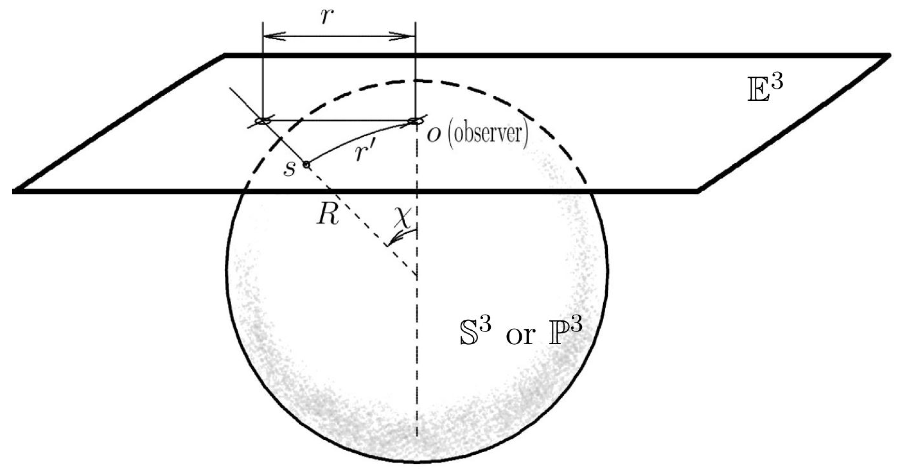
In Equations (1) and (3), is the natural radial coordinate as measured by the projective angle :
with the origin of coordinates at the observer’s location. This is schematically illustrated by Figure 1 where the main feature of elliptical space—the topological identification of antipodal points—is indicated by the vertical dashed line down from the observer’s location on the sphere . De Sitter introduced the coordinate transformation
in which r is the projection of the natural coordinate onto Euclidean or Lobachevsky space tangential to at the observer’s location o.
In the de Sitter’s solution, there is a global redshift effect (called the de Sitter effect) caused by time dilatation due to the metric coefficient
in the de Sitter metric (3). According to the definition , the de Sitter effect is the cosmological gravitational redshift for a homogeneously distributed energy density . Unlike the local gravitational redshift, which is always anisotropic from the observer’s perspective, the time dilatation due to the de Sitter effect is spherically symmetric around any arbitrary point of space (i.e., it is isotropic). This was de Sitter’s prediction of the cosmological redshift phenomenon [2] made a decade before its observational discovery in 1927 by Lemaître [6] and in 1929 by Hubble [11].
In the standard CDM cosmological model, the cosmological redshift is interpreted in terms of the motion of recession within the expanding space paradigm encoded by the Robertson-Walker’s time-dependent cosmic scale factor 1 of the FLRW metric [6,8,12,13]. The theoretical Hubble diagram based on the FLRW metric fits almost perfectly the observational data collected in the form of distance moduli of 1701 type-Ia supernovae in the Pantheon+ catalogue [14,15]. The goodness-of-fit parameter () of the CDM model to these data is pretty small: , the parameters and km , , , where this fit has been taken from [14].
By contrast, the computed for de Sitter’s model is very large (orders of magnitude), which can be explained by the fact that, in this model, the redshift-distance relationship is non-linear (quadratic) for small redshifts, whereas the observational redshift-distance relationship is strictly linear. That is why the de Sitter concept of global gravitational redshift in a static universe was abandoned, while the expanding-universe paradigm prevailed because the CDM model based on this paradigm successfully predicted and explained many observational phenomena, including the abundances of light elements in the Universe due to the Big-Bang nucleosynthesis, the isotropy and the power-spectrum of the Cosmic Microwave Background Radiation (CMBR), the power-spectrum of matter overdensities, and more.
However, despite the successes of the standard cosmological model during the last ninety years, there exist numerous observational facts casting doubt on the validity of this model. For example, the perturbative approach used in CDM to explain the structure-formation in the Universe is challenged by the fact that on scales below 100 Mpc the matter distribution in the Universe is extremely inhomogeneous, which is also related to some other issues with CDM [16]. Statistical studies of matter distribution [17,18,19] and of the CMBR [20] indicate that the Universe is fractal, which is in line with earlier theoretical studies of static cosmological models [21,22]. According to the CDM scenario, fractal distribution of matter is impossible. The more so, because of the difficulties of explaining within the CDM framework the origin of the largest-scale structures, such as a huge arc spanning 1 Gpc at redshift [23], large filaments or wall-like super-clusters with huge voids between them [24].
Other problems are related to the standard Big-Bang nucleosynthesis theory [25,26,27] and to the discrepancy (tension) between the values of the Hubble constant measured by different methods [28,29]. With respect to the latter issue, the present author found that the discrepancy is likely related to the fact that the CMBR data obtained by the Wilkinson Microwave Anisotropy Probe (WMAP) were contaminated by the irreducible intergalactic foreground [30], which was later confirmed by the Planck mission data [31,32]. Also consistent with those studies are findings of the CMBR hot and cold spots correlation with matter overdensities and underdensities [33,34]. The famous Cold Spot is notoriously inexplicable within the CDM framework. However, it was found to be physically related to the Eridanus supervoid [35,36], which links the CMBR origin with the matter distribution in the Universe.
The most recent and the most problematic issue in the standard cosmological model came from the James Webb Space Telescope (JWST) observations [37,38]. This telescope, capable of capturing images of galaxies with redshifts well above , discovered numerous high-redshift galaxies, which, by their properties turned out to be very similar to the galaxies in the local universe. These remote galaxies were found to be fully developed, despite having no time for their development from the beginning of the Universe as calculated within the CDM framework. The observed number densities of massive galaxies with redshifts above are also inconsistent with the galaxy formation models based on the CDM predictions [39].
These new observations indicate that the standard model’s prediction with respect to the age of the Universe is largely incorrect [40]. This dilemma can be solved by cosmological models that provide more time for high-redshift galaxies to evolve. There are recent publications discussing the possibility of increasing the estimated age of the Universe, either hypothesising the variability of fundamental constants [41] or by incorporating a “zero active mass” [42]. In this paper I discuss a similar possibility, that of increasing the Universe’s age, but without non-physical assumptions. My model uses de Sitter’s formulation with a global static gravitational redshift combined with the dynamic redshift based on a FLRW-like metric. The static part of the global redshift based on the Schwarzschild metric has already been discussed by the author elsewhere [43]. Here I resort to the combination of the Schwarzschild and FLRW metrics found in 1933 by G. C. McVittie [44]. In order to devise a strictly linear distance-to-redshift relationship, I make use of the main feature of elliptical space—the identification of its antipodal points, which is described in the next section.
2. Materials and Methods
2.1. The Origin of Coordinates
The global de Sitter effect [2] is due to the difference between the local (observer’s) and remote source coordinate reference frames. Another global gravitational redshift effect was discovered in 1947 by H. Bondi [45] who considered the Einstein metric (1) and found that there is a redshift proportional to the gravitational potential difference between the surface and the center of a ball of matter centred at the source and having radius equal to the source-to-observer distance. In both de Sitter and Bondi’s cases, the redshift-distance dependence is non-linear for small redshifts, which is at odds with observations.
In order to devise the required strictly-linear relationship between the source’s redshift and its distance to the observer, I resort to an unusual method of translating the origin of coordinates from the observer’s location to the observer’s antipodal point (to the best of the author’s knowledge, in all previous cosmological models, the origin of coordinates is at the observer’s location). For this method to work, one needs to endue the observer’s antipodal point with the Schwarzschild metric, which will provide the gravitational redshift effect.
One can achieve this by interpreting the main mathematical property of elliptical space—the identification of its antipodal points—as a physical, direct connection between these points. In terms of physics, the direct connection between remotely separated points of space is described by a general-relativistic structure found in 1935 by A. Einstein and N. Rosen [46]. This structure is called the Einstein-Rosen bridge or, more frequently, a “wormhole”. It has two “throats”, one in the vicinity of the observer (a near throat), and another at a very large distance from the observer (the far-throat). The wormhole connects two different spaces or two remote locations of the same space. Both of its throats are endued with the Schwarzschild metric, which can be used for calculating the gravitational redshift effect. In the case of elliptical space, the connection is between two antipodal points. But, in principle, other possible connections are not excluded.
Some authors argue that short-circuited connections between remotely separated points of space via wormholes explain the phenomenon of quantum entanglement of subatomic particles separated by large distances [47]. Wormholes were also considered by Morris, Thorne & Yurtsever as structures that allow instantaneous travel between remote regions of space [48]. However, the same authors, while further studying this possibility in detail, found that wormhole creation requires extremely large energies [49], which in terms of particle physics corresponds to extremely small distances. Thus, wormholes are likely to exist only on a scale-length of the order of the Planck-Wheeler length, cm. So, they are microscopic particles. There is a belief based on some past research (for example [50]) that wormholes are unstable and would instantly collapse once anything, such as a photon, traversed the wormholes’ horizon. But microscopic wormholes are not traversable, as they are the smallest possible entities of the Planck-Wheeler length with no singularities. This is also concurs with M.A. Markov’s suggestion [51] that the density of matter is always subject to an upper limit given by the expression
This follows logically because infinite energies are never observed in the Universe. As in the case of paper [50], practically the whole of the wormhole stability research is related to either wormhole traversability by matter or to the wormhole’s matter of field content (see [52,53,54] and others). The methods which are used include modified or extended theories of gravity [55], or quantum gravity [56]. None of these studies correspond to the ideas of Einstein, Rosen and Wheeler which posed the question about the origin of matter. Their microscopic wormholes are the smallest matter particles or matter particle ingredients. By definition they are stable and not traversable.
In elliptical space, the observer’s antipodal point is seen from the observer’s perspective as a sphere with a very large radius around the observer. So, what is seen as a point near the observer, is also seen as a global sphere spanning the whole steradians around. This is schematically illustrated by a diagram in Figure 2.
This diagram is a Poincaré disk conformally mapping the whole space to a (unit) disk with its circumference (the above mentioned global sphere) drawn in the form of a dot-dashed circle representing the antipodal point of the disk’s centre. The disk’s centre and its antipodal point (the circumference of the disk) are topologically identified as the same entity, i.e., they are physically connected via a wormhole.
A small dashed circle around the center of the Poincaré disk depicts the wormhole’s near-throat (a sphere) with its microscopic Schwartzschild radius. This small sphere corresponds to a large antipodal sphere at some distance from the disk’s circumference towards the interior of the disk. In Figure 2, it is shown as a large dashed circle at some distance from the disk edge. Although the observer is nearby and outside the small sphere, yet it is inside it because the antipodal image of this sphere surrounds the observer at a large distance.
2.2. Isotropy and Spherical Symmetry
A large volume of space around the observer, which includes the observer and all surrounding sources of light (the Sun, stars, galaxies, clusters of galaxies) is seen from the observer’s perspective as a very distant layer of space adjacent to the wormhole’s far-horizon. An essential aspect of this construct is its spherical symmetry for any arbitrary location in space. Assuming that the Universe is homogeneous on a large scale, one can show that for a sufficiently large neighbourhood around the observer all sources located within this volume are seen as a uniformly illuminated spherical layer bordering on the far-horizon. This layer is at a very large distance—much farther away from the observer than the limit of the observer’s neighbourhood. A possible mathematical description of a similar topological boundary around a point in a finite-volume set was conceived for both hyperbolic and elliptic geometries [57,58].
The remote horizons corresponding to each point within the neighbourhood region are at extremely large distances from the observer. This region might appear large, as it likely to include many clusters of galaxies. But cosmologically, its size is negligible as compared with the distances to the remote horizons of the points belonging to this region. In this way, a remote, almost spherically symmetric, collective horizon is formed around each point of elliptical space, thus, making any observer’s location equivalent to any other location. This conforms to the cosmological principle of isotropy.
2.3. Schwarzschild Metric
As just mentioned above, a sphere of neighbourhood matter with mass M surrounding the observer produces the effect of a global collective remote horizon, which is due to the Schwarzschild metric of the collective far-horizons of wormholes in the observer’s neighbourhood. The corresponding spacetime interval in Schwarzschild coordinates is [59]:
where . Here the metric coefficients and are
where is the gravitational (Schwarzschild) radius. This metric can also be expressed in isotropic coordinates as
or
We shall use this form when comparing this metric with the dynamic case. In the above formulae, r, and are spherical coordinates, G is the gravitational constant, c is the speed of light, and M is the mass of a very large sphere of matter surrounding the observer and producing the effect of a global remote horizon with its corresponding global gravitational redshift effect. As already mentioned, this effect is spherically symmetric for an arbitrary point of space. The mass M and the size of the sphere of matter are determined by the causal connectivity corresponding to the finite speed of the gravitational interaction.
In accord with our choice of the origin of coordinates at the observer’s antipodal point, any distance is measured from this antipodal point (which is a large sphere around the observer) towards the source () and towards the observer (). The gravitational radius is also measured from this sphere. These distances are indicated in Figure 2 by the pointers at the left edge of the sphere. Our purpose here is to find a relationship between the source redshift (z) and the source-to-observer distance (d):
Both and distances are unknown, but the latter can be expressed in terms of the distance . The parameter is also to be determined by using observational data. In the simplest Schwarzschild case, there are two free parameters: and . Both source and observer are located within the Schwartzschild metric (8) with its redshift-defining coefficient (9). So, the source’s redshift with respect to the observer is
or, by taking into account (9),
For simplicity, here we shall assume the parameter to be our distance unit. That is, we put . Later on, it can be converted to some common distance unit, such as Mpc. Thus,
By using (12) we replace by distance d:
obtaining
and, finally,
which is the required expression [in units of ] for calculating the theoretical source-to-observer distance for a given source redshift. For this redshift, distance d can be compared with the observed luminosity distance of a source. For this comparison, (18) has to be converted to the luminosity distance by using the squared -factor:
This factor is formed of three sub-factors accounting
- —for the loss of luminosity due to the cosmological redshift z;
- —for the lower rate at which the photons reach the observer because of the cosmological time dilatation;
- —for the photon path distortion (the coefficient of the metric).
If the distance unit is expressed in Mpc, then the theoretical distance modulus
is comparable with the observed distance moduli of type Ia supernovae (in stellar magnitudes).
2.4. McVittie Metric
The McVittie metric [44] describes the gravitational field of a mass point embedded into a dynamic FLRW metric with the scale factor
where H is a Hubble-like constant. It also includes the space curvature k, which I omit for simplicity. For the flat-universe case with , the McVittie metric in isotropic coordinates is
For the mass parameter , the McVittie metric coincides with the FLRW metric, and for the constant , it is reduced to the Schwarzschild metric (10) in isotropic coordinates. By putting
one gets the above expression in the form
which has the same form as Equation (11). Therefore, the luminosity distance (18) and (19), which is given in units of , can be used for the McVittie metric case, if one takes care of the time-dependent distance unit (23).
The time t in (21) can be calculated, to the first approximation, by using the static distance divided by the speed of light ( in units of ) with the first correcting sub-factor in (19) removed, because the loss of luminosity due to the cosmological redshift z is not applied when calculating the light-travel distance. That is,
Then Equation (20) can be re-written as
3. Results
3.1. Parameter Estimation
By applying the formulae derived above for the McVittie metric, one can calculate the theoretical luminosity distances and distance moduli corresponding to the redshifts of the type-Ia supernova. The comparison of these distance moduli with the observational data from the Pantheon+ catalogue is presented in Figure 3. The fit to the observational data is implemented by minimising the Pearson criterion for three parameters: , H and . The minimum with corresponds to the following parameter values:
the parameter being in units of , the Hubble-like parameter H in units of time of light travel across . The parameter is expressed in Mpc by the choice of coefficients in (26).
The salmon-colour points in Figure 3 represent the observational data from Pantheon+ [14]. The McVittie-based theoretical distance moduli for the minimum of are plotted in the form of a red dashed curve, and the CDM fit from [14] is shown as the black curve. The right panel of Figure 3 shows the differential data points with respect to the CDM theory (the thin horizontal line at ). The thick black curve on the right panel corresponds to the McVittie-based model with the parameter . By comparing the previously mentioned goodness-of-fit parameter with , one can see that the latter compares with observational data to the same level of accuracy as CDM. That is, both models are equivalent in terms of fitting their theoretical Hubble diagrams to observations within the redshift range covered by the Pantheon+ data (). However, for higher redshifts these models diverge. This is shown on the left panel of Figure 4, where the theoretical luminosity distances are plotted for the CDM model (the black curve) with the parameters and km , , from [14] and for the model based on the McVittie metric discussed here (the red curve) for the parameters (27)–(29). The black dashed curve is shown by comparison with the static version of the latter model, i.e., when .
3.2. Age of the Universe
Knowing the value (29) of the parameter , one can estimate the corresponding unit of time, , which is the light-crossing time of the distance (the speed of light, , is also expressed in units of ). With 1 Mpc [m] and [m/s]
the Hubble-like parameter H expressed in metric units reads
Thus , assuming the tolerance intervals from (28). The right panel of Figure 4 contrasts the look-back time based on this value (the red curve) with the look-back time based on the CDM model (, the black curve). The parameter H does not vary with time, as can be seen from (21):
In terms of frequencies, [], which constrains the age of the Universe to [s] or
assuming the tolerance intervals from (28).
4. Discussion
The cosmological model discussed here gives a new interpretation of the redshift-luminosity distance relationship for type-Ia supernovae. In this interpretation, the cosmological redshift is based on the static Schwarzschild metric embedded in the expanding FLRW metric, so the major part of the cosmological redshift is gravitational by its nature.
Therefore, the Hubble-like constant (31) is very small, and the corresponding age of the Universe (33) based on this constant is extremely large. The look-back time calculated by using the parameter (31) for with , is plotted on the right panel of Figure 4 (the red curve). It is about two orders of magnitude larger than the commonly accepted value.
By assuming the matter density and the radiation density one can evaluate their ratio at the end of the radiation-dominated era, when (see Figure 5).
The observational present-day ratio is indicated in Figure 5 by the horizontal dashed line. It corresponds to the time [yr] (the vertical dashed line). Presumably, this time is required for reaching the present-day matter-to-radiation density ratio. But it is at odds with the age of the Universe (33) previously estimated in Section 3.2.
The most likely reason for this inconsistency is that using the Friedmann equations for deriving the evolution of matter and radiation density in the discussed model is not fully adequate for achieving the observed ratio of these quantities. Further investigation of this question is required. This inconsistency, together with the smallness of the Hubble-like parameter [] of the McVittie metric, makes the discussed model practically indistinguishable from static. Therefore, here we have to pay regard to the observational challenges of a static cosmological model.
The standard cosmological model, CDM, based entirely on the dynamical interpretation of the cosmological redshift due to the recession velocities of galaxies, is very successful in explaining many other observational facts. Therefore, universal opinion tends to consider CDM as the best available model, while any alternative models, especially those based on the static (or almost static) metric must demonstrate that they can be, at least, as successful as CDM in explaining not only the redshift-luminosity distance relationship (discussed here), but all other observational facts, plus dark matter and dark energy, which are two essential components of CDM.
4.1. Dark Energy
The comparison of the theoretical distance moduli with observations (see Figure 3) demonstrates that the McVittie metric accounts fully for the extra dimming of the type Ia supernovae for , without invoking new concepts unknown to standard physics, such as hypothetical dark energy. The only viable way of linking dark energy to standard physics is by interpreting it as the vacuum energy of space, known from particle physics experiments. But there is a huge (about 120 orders of magnitude) discrepancy between the dark energy based on the cosmological constant devised from the extra dimming of the type-Ia supernovae and the vacuum energy known from particle physics experiments. This discrepancy cannot be resolved for CDM, but there is no such discrepancy in the model based on elliptical space with McVittie metric because the lambda-parameter of the latter model is interpreted as curvature and not as vacuum energy.
4.2. Dark Matter
As for dark matter, the observational evidence of its existence (e.g., the galaxy rotation curves) is as challenging for the CDM as for any other alternative model. So far, all the attempts to find any experimental evidence for dark matter particles have failed, while an alternative interpretation of galaxy rotation curves (the Modified Newtonian Dynamics theory, or MOND) continues to challenge CDM. The discussed McVittie metric-based model is closer to MOND in dealing with the dark matter issue (but this is a subject to be discussed in a separate paper).
As for the other observational facts, it is almost universally forgotten that, in the past, static cosmological models were not only supported by the same observational phenomena as CDM, but they predicted such phenomena existed. In the literature, there are plenty of papers discussing how static-universe models solve challenging observational facts in alternative ways to CDM. So, there is no need to review here these topics in detail. Below, I shall only briefly outline the most important of them.
4.3. Cosmological Redshift and the Cosmic Background
First of all, the cosmological redshift phenomenon was predicted by de Sitter for a static cosmological model well before the appearance of any dynamical cosmological model. Moreover, de Sitter warned in his 1917 paper that the lines of spectra systematically displaced towards the red might give rise to a spurious positive radial velocity interpretation [2]. In 1923, Eddington repeated this warning by writing that: in de Sitter’s theory, there is the general displacement of spectral lines to the red in distant objects due to the slowing down of atomic vibrations which would be erroneously interpreted as a motion of recession [60].
Then, in 1926, Eddington predicted a thermalised background radiation to exist with K for a static-Universe model [61]. Later, in 1937, a similar prediction with respect to the CMBR temperature K within a static Universe framework was proposed by W. Nernst [62]. Only much later, in 1953, G. Gamow made his prediction with respect to the CMBR and its temperature for the expanding-Universe model [63]. Several other authors, e.g., [64,65], were exploring CMBR properties in the 1990s and 2000s within the framework of a static universe model. The possibility of a local origin of the CMBR was already excluded by measurements of excitation lines in absorption features of quasar spectra [66], and by measuring the imprint of galaxy clusters on the CMBR via the Sunyaev-Zeldovich effect [67].
It turns out that the model discussed here unintentionally gives yet another alternative explanation of the CMBR. As was mentioned in §2.2, that all sources belonging to a large local volume of elliptical space around an arbitrary observer are visible as uniform light emitted from within a very distant layer of space adjacent to the collective wormhole far-horizon. This possibility is in tune with de Sitter’s comment about seeing “the back side of the Sun at the point of the heavens opposite to the Sun” in elliptical space [2].
For a local observer, this emission from a volume layer near the remote horizon is correspondingly redshifted due to the Schwarzschild metric. So, the energy (temperature) of this emission is scaled in accordance with the gravitational redshift formula , which is the same for the accelerated expansion of the Universe. Here is the highly redshifted temperature of photons produced by sources within the local sphere of matter surrounding the observer but coming to the observer from a remote layer of space adjacent to the far-horizon (in Figure 2, the local sphere of matter surrounding the observer is schematically indicated by the large-triangle pattern around the centre of the Poincaré disk, and the remote layer of space adjacent to the far-horizon is shown as the pattern of tiny triangles adjacent to the large dashed circle, the latter denoting the far-horizon location). This is a topic for discussion in a separate paper.
4.4. Abundances of Light Elements
The abundances of light elements in a static universe were explained by G.R. Burbidge and F. Hoyle [68,69], R. Salvaterra and A. Ferrara [70] and others, although there are some unresolved issues for static universe models. For example, according to the standard cosmological model, deuterium (2H) was created exclusively during the Big-Bang nucleosynthesis stage, after which it cannot be produced, and can only be destroyed in stars [71]. Therefore, its observed abundance is gradually diminishing. Similarly, lithium (7Li) is also regarded as having been produced during the Big-Bang nucleosynthesis. However, observations suggest its continuous enrichment due to cosmic-ray spallation [72].
There are other elements (e.g., boron) that cannot be produced in stars. But it is possible to explain their existence by the same cosmic-ray spallation or fusion reactions [73]. There are numerous studies of this process in the literature, e.g., [74,75,76], opening an alternative understanding of light element formation, which can be used by static cosmological models [69]. In fact, the same mechanism can also explain the production of 2H, and replenishment of 1H burned in nuclear reactions in stars. Since the energies of cosmic rays can be as high as eV, they can produce spallation fragments even from 4He [77]. Highly energetic neutrinos can also spallate 4He [78]. Reactions of this kind are regularly observed in laboratory experiments [79].
4.5. Cosmic Structure
According to the classical scenarios, structure formation in static universe models occurs due to the mechanism of gravitational instability. Initial fluctuations in the homogeneous gas of primordial hydrogen grow exponentially into large-scale structures [82,83]. In the early years of cosmology, these scenarios agreed with observations. But, when Eddington showed in 1930 that Einstein’s static model of the Universe was unstable [84], static models fell out of fashion.
Only fourty yeas later, Eddington’s verdict was overturned by N. Rosen [85], who rehabilitated the Einstein static model and proved its stability. This reopened the possibility for solving the problem of structure formation in static cosmological models.
In these models, matter clumping was found to be fractal [21,22], which is confirmed by statistical studies of CMBR maps [20] and of the matter distribution in the Universe [17,18,19]. By contrast, according to the CDM scenario, matter distribution cannot be fractal. The origin of the largest scale structures in the universe (the filaments and wall-like super-clusters, with huge voids between them), is not yet entirely understood from the point of view of CDM.
4.6. Angular Sizes
Static and dynamic cosmological models predict different angular sizes on the sky of remote objects whose linear sizes are known (standard rulers). For example, in an expanding-universe model, the angular size of a remote galaxy varies in such a way that as the galaxy is moved from lower to higher redshifts its angular size decreases at first to a minimum, then increases. This theoretical prediction of the standard cosmological model with is illustrated by the black solid curve in Figure 6. For an empty universe with , the angular size of a standard ruler always decreases (the black dotted curve).
Galaxies are not the standard rulers—their sizes vary significantly. But one can check how most of them appear at different redshifts. The theoretical curves plotted in Figure 6 correspond to a medium-size galaxy of 15 kpc. The low-redshift galaxy sizes vary about this value. Galaxies of the same size at redshift appear to have an average angular diameter of arcsec. This is slightly smaller than is predicted by the CDM-model for a 15 kpc galaxy. So, one can conclude that galaxies evolve in time and grow by merging with other galaxies.
At higher redshifts, , the observed angular sizes of galaxies continue to decrease (the red points in this plot correspond to the JWST observations). They match neither the CDM, nor the empty universe model’s predictions for kpc. Accordingly, the calculated physical sizes of these galaxies at turn out to be very small.
At first glance, this result seems sensible, because the prediction of the Standard Cosmological Model is exactly this progression in size, from being small at large redshifts, when the Universe was very young, to large sizes at smaller redshifts. But there is a problem here: small galaxies at the initial stages of their evolution are supposed to be irregular and to have small masses.
In contradiction to this, the high-redshift galaxies are found by the JWST to be well-evolved, symmetrical and having sometimes disks and bulges. Moreover, their masses turn out to be very large, similar to the masses of nearby galaxies. In addition, such galaxies must have evolved within the very short time available since the beginning of the Universe, i.e., a few hundred million years assuming the CDM Big Bang model. Moreover, the chemical composition of these galaxies and the dust in them is the same as in nearby galaxies.
Imagine a well-evolved galaxy, similar in shape, mass and chemical composition to our Milky Way, but being just a th of the Milky Way’s size. This looks very unnatural. Now, if one looks at the predictions for the sizes of the galaxies made by the model with the McVittie metric discussed here (the red dashed curve in Figure 6) one finds that these galaxies are actually pretty normal, by being ∼15 kPc in their sizes or more. The model discussed here provides plenty of time for these galaxies to evolve (two orders of magnitude more than CDM).
5. Conclusions
As we have seen, the McV and CDM models are equivalent for the redshift range : their goodness-of-fit criteria () are identical. But for larger redshifts, these two models diverge (see the right panel of Figure 3). According to this scenario, if newly-discovered high-redshift supernova appear dimmer than what is predicted for them by the CDM model, then the McVittie metric of elliptical space would need to be considered more seriously.
Funding
This research received no external funding.
Data Availability Statement
The data used for preparing this manuscript are available at https://pantheonplussh0es.github.io (accessed on 27 March 2024).
Acknowledgments
This research has made use of the following archive: The Pantheon+ Type Ia supernova distance moduli from [14,15] I am also acknowledging the use of the cosmoFns software package version 1.1-1 developed by Andrew Harris and available at the following web page: github.com/cran/cosmoFns (accessed on 27 March 2024). I would like to thank Paul Kuin, Leslie Morrison, Alice Breeveld, Victor Tostykh and Mat Page for useful discussions on the matters in this paper.
Conflicts of Interest
The author declares no conflict of interest.
Abbreviations
The following abbreviations are used in this manuscript:
| CMBR | Cosmic Microwave Background Radiation |
| dS | de Sitter (metric) |
| FLRW | Friedmann-Lemaitre-Robertson-Walker (metric) |
| JWST | James Webb Space Telescope |
| CDM | Lambda-Cold-Dark-Matter (cosmological model) |
| McV | McVittie (metric) |
| MOND | Modified Newtonian Dynamics (theory) |
| SN | supernova |
| WMAP | Wilkinson Microwave Anisotropy Probe. |
| 1 | ; being the Hubble constant. |
References
- Hamilton, W.R. On quaternions; or on a new system of imaginaries in algebra. Philos. Ser. 1844, 10–13, 241–246. [Google Scholar] [CrossRef]
- De Sitter, W. On Einstein’s theory of gravitation, and its astronomical consequences. Third paper. Mon. Not. R. Astron. Soc. 1917, 78, 3–28. [Google Scholar] [CrossRef]
- Einstein, A. Kosmologische betrachtungen zur allgemeinen Relativitätstheorie. Sitz. Preuss. Akad. Wiss. Phys. 1917, VL, 142–152. [Google Scholar]
- Newcomb, S. Elementary theorems relating to the geometry of a space of three dimensions and of uniform positive curvature in the fourth dimension. J. Reine Angew. Math. 1877, LXXXIII, 293–299. [Google Scholar]
- Schwarzschild, K. Ueber das zulässige Krümmunsmass des Raumes. Vierteljahrssch. Astr. Ges. 1900, XXXV, 337–347. [Google Scholar]
- Lemaître, G. Un univers homogène de masse constante et de rayon croissant rendant compte de la vitesse radiale des nébuleuses extra-galactiques. Ann. Soc. Sci. Brux. A. 1927, 47, 49–59. [Google Scholar]
- Tolman, R.C. On the estimation of distances in a curved universe with a non-static line element. Proc. Natl. Acad. Sci. USA 1930, 16, 511–520. [Google Scholar] [CrossRef]
- Robertson, H.P. Kinematics and world structure I. Astrophys. J. 1935, 82, 284–301. [Google Scholar] [CrossRef]
- Robertson, H.P. Kinematics and World-Structure II. Astrophys. J. 1936, 83, 187–201. [Google Scholar] [CrossRef]
- Robertson, H.P. Kinematics and World-Structure III. Astrophys. J. 1936, 83, 257–271. [Google Scholar] [CrossRef]
- Hubble, E. A relation between distance and radial velocity among extragalactic nebulae. Proc. Natl. Acad. Sci. USA 1929, 15, 168–173. [Google Scholar] [CrossRef] [PubMed]
- Friedmann, A. Über die Krümmung des Raumes. Z. Phys. A 1922, 10, 377–386. [Google Scholar] [CrossRef]
- Walker, A.G. On Milne’s theory of world-structure. Proc. Lond. Math. Soc. Ser. 2 1937, 42, 90–127. [Google Scholar] [CrossRef]
- Brout, D.; Scolnic, D.; Popovic, B.; Riess, A.G.; Zuntz, J.; Kessler, R.; Carr, A.; Davis, T.M.; Hinton, S.; Jones, D.; et al. The Pantheon+ Analysis: Cosmological Constraints. Astrophys. J. 2022, 938, 110. [Google Scholar] [CrossRef]
- Scolnic, D.; Brout, D.; Carr, A.; Riess, A.G.; Davis, T.M.; Dwomoh, A.; Jones, D.O.; Ali, N.; Charvu, P.; Chen, R.; et al. The Pantheon+ Analysis: The Full Dataset and Light-Curve Release. Astrophys. J. 2022, 938, 113. [Google Scholar] [CrossRef]
- Kroupa, P.; Pawlowski, M.; Milgrom, V. The failures of the standard model of cosmology require a new paradigm. Int. J. Mod. Phys. D 2012, 21, 1230003. [Google Scholar] [CrossRef]
- Coleman, P.H.; Pietronero, L. The fractal structure of the universe. Phys. Rep. 1992, 213, 311–389. [Google Scholar] [CrossRef]
- Gaite, J. The fractal geometry of the cosmic web and its formation. Adv. Astron. 2019, 2019, 6587138. [Google Scholar] [CrossRef]
- Teles, S.; Lopes, A.R.; Ribeiro, M.B. Galaxy distributions as fractal systems. Eur. Phys. J. C 2021, 82, 896. [Google Scholar] [CrossRef]
- Mylläri, A.A.; Raikov, A.A.; Orlov, V.V.; Tarakanov, P.A.; Yershov, V.N.; Yezhkov, M.Y. Fractality of isotherms of the Cosmic Microwave Background based on data from the Planck Spacecraft. Astrophysics 2016, 59, 31–37. [Google Scholar] [CrossRef]
- Baryshev, Y. The hierarchical structure of metagalaxy a review of problems. Rep. Sp. Aph. Obs. Rus. Acad. Sci. 1981, 14, 24–43. [Google Scholar]
- Baryshev, Y.; Teerikorpi, P. The Discovery of Cosmic Fractals; World Scientific: Singapore, 2002; 408p. [Google Scholar]
- Lopez, A.L.; Clowes, R.G.; Williger, G.M. A giant arc on the sky. Mon. Not. R. Astron. Soc. 2022, 516, 1557–1572. [Google Scholar] [CrossRef]
- Yadav, J.K.; Bagla, J.S.; Khai, N. Fractal dimension as a measure of the scale of homogeneity. Mon. Not. R. Astron. Soc. 2010, 405, 2009–2015. [Google Scholar] [CrossRef]
- Sargent, W.L.W.; Searle, L. The interpretation of the helium weakness in halo stars. Astrophys. J. 1967, 150, L33–L37. [Google Scholar] [CrossRef]
- Terlevich, E.; Terlevich, R.; Skillman, E.; Stepanian, J.; Lipovetskii, V. The extremely low He abundance of SBS:0335-052. In Elements and the Cosmos; Edmunds, M.G., Terlevich, R., Eds.; Cambridge University Press: Cambridge, UK, 2010; pp. 21–27. [Google Scholar]
- Izotov, Y.I.; Thuan, T.X. The primordial abundance of 4He: Evidence for non-standard Big Bang nucleosynthesis. Astrophys. J. 2010, 710, L67–L71. [Google Scholar] [CrossRef]
- Di Valentino, E.; Melchiorri, A.; Silk, J. Planck evidence for a closed Universe and a possible crisis for cosmology. Nat. Astron. 2020, 4, 196–203. [Google Scholar] [CrossRef]
- Yang, W.; Giarè, W.; Pan, S.; Di Valentino, E.; Melchiorri, A.; Silk, J. Revealing the effects of curvature on the cosmological models. Phys. Rev. D 2023, 107, 063509. [Google Scholar] [CrossRef]
- Yershov, V.N.; Orlov, V.V.; Raikov, A.A. Correlation of supernova redshifts with temperature fluctuations of the cosmic microwave background. Mon. Not. R. Astron. Soc. 2012, 423, 2147–2152. [Google Scholar] [CrossRef]
- Yershov, V.N.; Orlov, V.V.; Raikov, A.A. Possible signature of distant foreground in the Planck Data. Mon. Not. R. Astron. Soc. 2014, 445, 2440–2445. [Google Scholar] [CrossRef]
- Yershov, V.N.; Raikov, A.A.; Lovyagin, N.Y.; Kuin, N.P.M.; Popova, E.A. Distant foreground and the Planck-derived Hubble constant. Mon. Not. Roy. Astron. Soc. 2020, 492, 5052–5056. [Google Scholar] [CrossRef]
- Granett, B.R.; Neyrinck, M.C.; Szapudi, I. An imprint of superstructures on the microwave background due to the integrated Sachs-Wolfe effect. Astrophys. J. 2008, 683, L99–L102. [Google Scholar] [CrossRef]
- Cai, Y.-C.; Neyrinck, M.C.; Szapudi, I.; Cole, S.; Frenk, C.S. A possible cold imprint of voids on the microwave background radiation. Astrophys. J. 2014, 786, 110. [Google Scholar] [CrossRef]
- Kovács, A.; García-Bellido, J. Cosmic troublemakers: The Cold Spot, the Eridanus supervoid, and the Great Walls. Mon. Not. Roy. Astron. Soc. 2016, 462, 1882–1893. [Google Scholar] [CrossRef]
- Kovács, A.; Jeffrey, N.; Gatti, M.; Chang, C.; Whiteway, L.; Hamaus, N.; Lahav, O.; Pollina, G.; Bacon, D.; Kacprzak, T.; et al. The DES view of the Eridanus supervoid and the CMB cold spot. Mon. Not. Roy. Astron. Soc. 2021, 510, 216–229. [Google Scholar] [CrossRef]
- Labbé, I.; van Dokkum, P.; Nelson, E.; Bezanson, R.; Suess, K.A.; Leja, J.; Brammer, G.; Whitaker, K.; Mathews, E.; Stefanon, M.; et al. A population of red candidate massive galaxies ∼600 Myr after the Big Bang. Nature 2023, 616, 266–269. [Google Scholar] [CrossRef] [PubMed]
- Yan, H.; Ma, Z.; Ling, C.; Cheng, C.; Huang, J.-S. First batch of z ≈ 11–20 candidate objects revealed by the James Webb Space Telescope early release observations on SMACS 0723–73. Astrophys. J. Lett. 2023, 942, L9. [Google Scholar] [CrossRef]
- Castellano, M.; Fontana, A.; Treu, T.; Merlin, E.; Santini, P.; Bergamini, P.; Grillo, C.; Rosati, P.; Acebron, A.; Leethochawalit, N.; et al. Early results from GLASS-JWST. XIX. A high density of bright galaxies at z ≈ 10 in the A2744 region. Astrophys. J. Lett. 2023, 948, L14. [Google Scholar] [CrossRef]
- Lovyagin, N.; Raikov, A.; Yershov, V.; Lovyagin, Y. Cosmological model tests with JWST. Galaxies 2022, 10, 108. [Google Scholar] [CrossRef]
- Gupta, R.P. JWST early Universe observations and ΛCDM cosmology. Mon. Not. R. Astron. Soc. 2023, 524, 3385–3395. [Google Scholar] [CrossRef]
- Melia, F. The cosmic timeline implied by the JWST high-redshift galaxies. Mon. Not. R. Astron. Soc. 2023, 521, L85–L89. [Google Scholar] [CrossRef]
- Yershov, V.N. Fitting type Ia supernova data to a cosmological model based on Einstein–Newcomb–De Sitter space. Universe 2023, 9, 24. [Google Scholar] [CrossRef]
- MvVittie, G.C. The mass-particle in an expanding Universe. Mon. Not. R. Astron. Soc. 1933, 93, 325–339. [Google Scholar] [CrossRef]
- Bondi, H. Spherically symmetrical models in general relativity. Mon. Not. R. Astron. Soc. 1947, 107, 410–425. [Google Scholar] [CrossRef]
- Einstein, A.; Rosen, N. The Particle Problem in the General Theory of Relativity. Phys. Rev. 1935, 48, 73–77. [Google Scholar] [CrossRef]
- Tamburini, F.; Licata, I. General relativistic wormhole connections from Planck-scales and the ER = EPR conjecture. Entropy 2020, 22, 3. [Google Scholar] [CrossRef] [PubMed]
- Morris, M.S.; Thorne, K.S. Wormholes in spacetime and their use for interstellar travel: A tool for teaching general relativity. Am. J. Phys. 1988, 56, 395–412. [Google Scholar] [CrossRef]
- Morris, M.S.; Thorne, K.S.; Yurtsever, U. Wormholes, time machines. and the weak energy condition. Phys. Rev. Lett. 1988, 61, 1446–1449. [Google Scholar] [CrossRef] [PubMed]
- Fuller, R.W.; Thorne, K.S. Causality and multiply connected space-time. Phys. Rev. 1962, 128, 919–929. [Google Scholar] [CrossRef]
- Markov, M.A. Limiting density of matter as a universal law of nature. JETP Lett. 1982, 36, 214–216. [Google Scholar]
- Bronnikov, K.; Lipatova, L.; Novikov, I.; Shatskiy, A. Example of a stable wormhole in general relativity. Grav. Cosmol. 2013, 19, 269–274. [Google Scholar] [CrossRef]
- Blázquez-Salcedo, J.-L.; Knoll, C.; Radu, E. Traversable wormholes in Einstein-Dirac-Maxwell theory. Phys. Rev. Lett. 2021, 126, 101102. [Google Scholar] [CrossRef]
- Koiran, P. Infall time in the Eddington–Finkelstein metric, with application to Einstein–Rosen bridges. Int. J. Mod. Phys. 2021, 30, 2150106. [Google Scholar] [CrossRef]
- Rosa, J.L. Double gravitational layer traversable wormholes in hybrid metric-Palatini gravity. Phys. Rev. D 2022, 104, 064002. [Google Scholar] [CrossRef]
- Cox, P.H.; Harms, B.C.; Hou, S. Stability of Einstein-Maxwell-Kalb-Ramond wormholes. Phys. Rev. D 2016, 93, 044014. [Google Scholar] [CrossRef]
- Battista, E.; Esposito, G. What is a reduced boundary in general relativity? Int. J. Mod. Phys. 2021, 30, 2150050. [Google Scholar] [CrossRef]
- Battista, E.; Esposito, G. Discontinuous normals in non-euclidean geometries and two-dimensional gravity. Symmetry 2022, 14, 1979. [Google Scholar] [CrossRef]
- Schwarzschild, K. Über das Gravitationsfeld eines Massenpunktes nach der Einsteinschen Theorie. Sitz. Preuss. Akad. Wiss. 1916, 3, 189–196. [Google Scholar]
- Eddington, A.S. The Mathematical Theory of Relativity; Cambridge University Press: Cambridge, UK, 1923; p. 161. [Google Scholar]
- Eddington, A.S. Internal Constitution of the Stars; Cambridge University Press: Cambridge, UK, 1926; p. 407. [Google Scholar]
- Nernst, W. Weitere prüfung der annahme lines stationären zustandes im weltall. Zeit. Phys. 1937, 106, 633–661. [Google Scholar] [CrossRef]
- Gamow, G. The expanding universe and the origin of galaxies. Kgl. Dan. Vidensk. Selsk. Mat. Fys. Medd. 1953, 27, 3–15. [Google Scholar]
- Baryshev, Y.V.; Raikov, A.A.; Tron, A.A. Microwave background radiation and cosmological large numbers. Astron. Astroph. Trans. 1996, 10, 135–138. [Google Scholar] [CrossRef]
- Cirkovic, M.M.; Perovic, S. Alternative explanations of the Cosmic Microwave Background: A historical and an epistemological perspective. Stud. Hist. Philos. Mod. Phys. 2018, 62, 1–18. [Google Scholar] [CrossRef]
- Muller, S.; Beelen, A.; Black, J.H.; Curran, S.J.; Horellou, C.; Aalto, S.; Combes, F.; Guélin, M.; Henkel, C. A precise and accurate determination of the cosmic microwave background temperature at z = 0.89. Astron. Astrophys. 2013, 551, A109. [Google Scholar] [CrossRef]
- Luzzi, G.; Shimon, M.; Lamagna, L.; Rephaeli, Y.; De Petris, M.; Conte, A.; De Gregori, S.; Battistelli, E.S. Redshift dependence of the cosmic microwave background temperature from Sunyaev-Zeldovich measurements. Astron. J. 2009, 705, 1122–1128. [Google Scholar] [CrossRef]
- Burbidge, G.R. Was there really a Big Bang? Nature 1971, 233, 36–40. [Google Scholar] [CrossRef] [PubMed]
- Burbidge, G.R.; Hoyle, F. The origin of helium and the other light elements. Astrophys. J. 1998, 509, L1–L3. [Google Scholar] [CrossRef]
- Salvaterra, R.; Ferrara, A. Is primordial 4He truly from the Big Bang? Mon. Not. R. Astron. Soc. 2003, 340, L17–L20. [Google Scholar] [CrossRef]
- Pagel, B.E.J. Abundances of elements of cosmological interest. Phil. Trans. R. Soc. Lond. A 1982, 307, 19–35. [Google Scholar] [CrossRef]
- Spite, F.; Spite, M. Abundances of Lithium in unevolved halo stars and old disk stars: Interpretations and consequences. Astron. Astrophys. 1982, 115, 357–366. [Google Scholar]
- Reeves, H.; Fpwler, W.A.; Hoyle, F. Galactic cosmic ray origin of Li, Be and B in stars. Nature 1970, 226, 727–729. [Google Scholar] [CrossRef]
- Austin, S.M. The creation of the light elements—Cosmic rays and cosmology. Progr. Part. Nucl. Phys. 1981, 7, 1–46. [Google Scholar] [CrossRef]
- Silverberg, R.; Tsao, C.H. Spallation processes and nuclear interaction products of cosmic rays. Phys. Rep. 1990, 191, 351–408. [Google Scholar] [CrossRef]
- Olive, K.A.; Schramm, D.N. Astrophysical 7Li as a product of Big Bang nucleosynthesis and galactic cosmic-ray spallation. Nature 1992, 360, 439–442. [Google Scholar] [CrossRef]
- Yamanaka, M.; Jittoh, T.; Kazunori Kohri, K.; Koike, M.; Sato, J.; Sugai, K.; Yazaki, K. Big-bang nucleosynthesis with a long-lived CHAMP including He4 spallation process. J. Phys. Conf. Ser. 2014, 485, 012020. [Google Scholar] [CrossRef]
- Meyer, B.S.; Woosley, S.E.; Hoffman, R.D.; Mathews, G.J.; Wilson, J.R. Neutrino spallation reactions on 4He and the r-process. AIP Conf. Proc. 1995, 327, 441–445. [Google Scholar] [CrossRef]
- Oliver, B.M.; James, M.R.; Garner, F.A.; Maloy, S.A. Helium and hydrogen generation in pure metals irradiated with high-energy protons and spallation neutrons in LANSCE. J. Nucl. Mat. 2002, 307–311, 1471–1477. [Google Scholar] [CrossRef]
- Abbott, B.P.; Abbott, R.; Abbott, T.D.; Acernese, F.; Ackley, K.; Adams, C.; Adams, T.; Addesso, P.; Adhikari, R.X.; Adya, V.B.; et al. [LIGO, Virgo and Other Collaborations]. Multi-messenger Observations of a Binary Neutron Star Merger. Astrophys. J. 2017, 848, L12. [Google Scholar] [CrossRef]
- Gompertz, B.P.; Ravasio, M.E.; Nicholl, M.; Levan, A.J.; Metzger, B.D.; Oates, S.R.; Lamb, G.P.; Fong, W.-F.; Malesani, D.B.; Rastinejad, J.C.; et al. The case for a minute-long merger-driven gamma-ray burst from fast-cooling synchrotron emission. Nat. Astron. 2022, 7, 67–79. [Google Scholar] [CrossRef]
- Jeans, J. Astronomy and Cosmogony; Cambridge University Press: Cambridge, UK, 1928; 428p. [Google Scholar] [CrossRef]
- Hoyle, F. On the fragmentation of gas clouds into galaxies and stars. Astrophys. J. 1953, 118, 513–528. [Google Scholar] [CrossRef]
- Eddington, A.S. On the instability of Einstein’s spherical world. Mon. Not. R. Astron. Soc. 1930, 90, 668–678. [Google Scholar] [CrossRef]
- Rosen, N. Static universe and cosmic field. Ann. Math. Pure Appl. 1970, 14, 305–308. [Google Scholar] [CrossRef]
- Yang, L.; Morishita, T.; Leethochawalit, N.; Castellano, M.; Calabro, A.; Treu, T.; Bonchi, A.; Fontana, A.; Mason, C.; Merlin, E.; et al. Early results from GLASS-JWST. V: The first rest-frame optical size-luminosity relation of galaxies at z > 7. Astrophys. J. Lett. 2022, 938, L17. [Google Scholar] [CrossRef]
- Finkelstein, S.L.; Bagley, M.B.; Haro, P.A.; Dickinson, M.; Ferguson, H.F.; Kartaltepe, J.S.; Papovich, C.; Burgarella, D.; Kocevski, D.D.; Iyer, K.G.; et al. A long time ago in a galaxy rar, far away: A candidate z ∼ 14 galaxy in early JWST CEERS imaging. Astrophys. J. Lett. 2022, 940, L55. [Google Scholar] [CrossRef]
- Chen, Z.; Stark, D.P.; Endsley, R.; Topping, M.; Whitler, L.; Charlot, S. JWST/NIRCam observations o stars and HII regions in z ∼ 6–8 galaxies: Properties of star forming complexes on 150 pc scales. Mon. Not. R. Astron. Soc. 2023, 518, 5607–5619. [Google Scholar] [CrossRef]
- Ono, Y.; Harikane1, Y.; Ouchi, M.; Yajima, H.; Abe, M.; Isobe, Y.; Shibuya, T.; Wise, J.H.; Zhang, Y.; Nakajima, K.; et al. Morphologies of galaxies at z = 9–12 uncovered by JWST/NIRCam imaging: Cosmic size evolution and an identification of an extremely compact bright galaxy at z ∼ 12. Astrophys. J. 2023, 951, 72. [Google Scholar] [CrossRef]
- Wu, Y.; Cai, Z.; Sun, F.; Bian, F.; Lin, X.; Li, Z.; Li, M.; Bauer, F.E.; Egami, E.; Fan, X.; et al. The identification of a dusty grand design spiral galaxy at z=3.06 with JWST and ALMA. Astrophys. J. Lett. 2023, 942, L1. [Google Scholar] [CrossRef]
- Atek, H.; Shuntov, M.; Furtak, L.J.; Richard, J.; Kneib, J.-P.; Mahler, G.; Zitrin, A.; McCracken, H.J.; Charlot, S.; Chevallard, J.; et al. Revealing Galaxy Candidates out to ∼16 with JWST Observations of the Lensing Cluster SMACS0723. Mon. Not. R. Astron. Soc. 2023, 519, 1201–1220. [Google Scholar] [CrossRef]
- Tacchella, S.; Johnson, B.D.; Robertson, B.E.; Carniani, S.; D’Eugenio, F.; Kumari, N.; Maiolino, R.; Nelson, E.J.; Suess, K.A.; Übler, H.; et al. JWST NIRCam+NIRSpec: Interstellar medium and stellar populations of young galaxies with rising star formation and evolving gas reservoirs. Mon. Not. R. Astron. Soc. 2023, 522, 6236–6249. [Google Scholar] [CrossRef]
- Naidu, R.P.; Oesch, P.A.; Setton, D.J.; Matthee, J.; Conroy, C.; Johnson, B.D.; Weaver, J.R.; Bouwens, R.J.; Brammer, G.B.; Dayal, P.; et al. Schrodinger’s galaxy candidate: Puzzlingly luminous at z ≈ 17, or dusty/quenched at z ≈ 5? arXiv 2022, arXiv:2208.02794. [Google Scholar]
- Naidu, R.P.; Oesch, P.A.; van Dokkum, P.; Nelson, E.J.; Suess, K.A.; Brammer, G.; Whitaker, K.E.; Illingworth, G.; Bouwens, R.; Tacchella, S.; et al. Two remarkably luminous galaxy candidates at z ≈ 11–13 revealed by JWST. Astrophys. J. Lett. 2022, 940, L14. [Google Scholar] [CrossRef]
- Adams, N.J.; Conselice, C.J.; Ferreira, L.; Austin, D.; Trussler, J.; Juodzbalis, I.; Wilkins, S.M.; Caruana, J.; Dayal, P.; Verma, A.; et al. Discovery and properties of ultra-high redshift galaxies (9 < z < 12) in the JWST ERO SMACS 0723 Field. Mon. Not. R. Astron. Soc. 2023, 518, 4755–4766. [Google Scholar] [CrossRef]
- Salzer, J.J.; MacAlpine, G.M.; Boroson, T.A. Oservations of a complete sample of emission-line galaxies: I. Astrophys. J. Suppl. 1989, 70, 447–477. [Google Scholar] [CrossRef]
- Koo, D.C.; Bershady, M.A.; Wirth, G.D.; Stanford, S.A.; Majewski, S.R. HST images of very compact blue galaxies at z ∼ 0.2. Astrophys. J. 1994, 427, L9–L12. [Google Scholar] [CrossRef]
- Guzman, R.; Gallego, J.; Koo, D.C.; Phillips, A.C.; Lowenthal, J.D.; Faber, S.M.; Illingworth, G.D.; Vogt, N.P. The nature of compact galaxies in the Hubble Deep Field. I. Global properties. Astrophys. J. 1997, 489, 543–558. [Google Scholar] [CrossRef]
- Zirm, A.W.; van der Wel, A.; Franx, M.; Zirm, A.W.; van der Wel, A.; Franx, M.; Labbe, I.; Trujillo, I.; van Dokkum, P.; Toft, S.; et al. NICMOS imaging of DRGs in the HDF-S: A relation between star-formation and size at z ∼ 2.5. Astrophys. J. 2007, 656, 66–72. [Google Scholar] [CrossRef]
- Hathi, N.P.; Malhotra, S.; Rhoads, J.E. Starburst intensity limit of galaxies at z ∼ 5–6. Astrophys. J. 2008, 678, 686–693. [Google Scholar] [CrossRef]
- Van der Wel, A.; Franx, M.; van Dokkum, P.G.; Skelton, R.E.; Momcheva, I.G.; Whitaker, K.E.; Brammer, G.B.; Bell, E.F.; Rix, H.-W.; Wuyts, S.; et al. 3D-HST+CANDELS: The evolution of the galaxy size-mass distribution since z = 3. Astrophys. J. 2014, 788, 28. [Google Scholar] [CrossRef]
- Bowler, R.A.A.; Dunlop, J.S.; McLure, R.J.; McLeod, D.J. Unveiling the nature of bright z ≈ 7 galaxies with the Hubble Space Telescope. Mon. Not. R. Astron. Soc. 2017, 466, 3612–3635. [Google Scholar] [CrossRef]
- Bridge, J.S.; Holwerda, B.W.; Stefanon, M.; Bouwens, R.J.; Oesch, P.A.; Trenti, M.; Bernard, S.R.; Bradley, L.D.; Illingworth, G.D.; Kusmic, S.; et al. The super eight galaxies: Properties of a sample of very bright galaxies at 7 < z < 8. Astrophys. J. 2019, 882, 42. [Google Scholar] [CrossRef]
- Bagley, M.B.; Finkelstein, S.L.; Rojas-Ruiz, S.; Diekmann, J.; Finkelstein, K.D.; Song, M.; Papovich, C.; Somerville, R.S.; Baronchelli, I.; Dai, Y.S.; et al. Bright z ∼ 9 galaxies in parallel: The bright end of the rest-UV luminosity function from HST parallel programs. arXiv 2022, arXiv:2205.12980. [Google Scholar] [CrossRef]
- Zavala, J.A.; Casey, C.M.; Spilker, J.; Tadaki, K.-I.; Tsujita, A.; Champagne, J.; Iono, D.; Kohno, K.; Manning, S.; Montana, A.; et al. Probing cold gas in a massive, compact star-forming galaxy at z = 6. Astrophys. J. 2022, 933, 242. [Google Scholar] [CrossRef]
Figure 1.
Embedding diagram (one spatial dimension suppressed) depicting spherical or elliptical space of constant positive curvature with two antipodal points topologically identified (the vertical dashed connection between two poles). The tangential Euclidean space at the observer’s location o indicates the local coordinate reference frame. Distances along the natural spatial coordinate of are measured by the projective angle , with . The corresponding projective distance to the source s in is .

Figure 2.
Poincaré disk illustrating the concept of the spherical symmetry of wormhole far-throats around each point in elliptical space. The disk spans the whole of the sphere, the central point of the disk (the centre of the wormhole’s near-throat) being near the observer’s location o. A small dashed circle around the central point denotes the event horizon of the near-throat, and the larger dashed circle denotes the corresponding event horizon of the wormhole’s far throat. The distances , and are measured from the centre of the far-throat (the outer dot-dashed circle).

Figure 3.
Left: comparison of theoretical distance moduli (the red and black curves) with the observational distance moduli of 1701 type-Ia supernovae from the Pantheon+ catalogue (the salmon-colour points). The dashed red curve corresponds to the model based on the McVittie metric, while the solid black curve is the reference corresponding to the standard CDM cosmological model. Right: the same data in detail, plotted in the form of the residuals with respect to the CDM-reference, which is thus the horizontal line at . The abscissae in both plots correspond to source redshifts z.

Figure 4.
Left: theoretical luminosity distances (in Gpc) as predicted by the CDM model (the black curve), the model based on the McVittie metric (McV, the red curve), and the McV model with the Hubble-like parameter (the dashed black curve). Right: look-back time for the CDM model with the Hubble parameter (black curve) and for the model based on the McVittie metric with its Hubble-like parameter (red curve).

Figure 5.
Matter to radiation density ratio from the end of the radiation-dominated era, as calculated from the model based on the McVittie metric by using the parameter (31).
Figure 5.
Matter to radiation density ratio from the end of the radiation-dominated era, as calculated from the model based on the McVittie metric by using the parameter (31).

Figure 6.
Angular sizes of galaxies with different redshifts. The red points indicate the data obtained by various authors from the very high-redshift observations made by the JWST during it’s first year in space [86,87,88,89,90,91,92,93,94,95]. The black points indicate the data obtained before JWST [96,97,98,99,100,101,102,103,104,105]. The theoretical curves are calculated for a medium-size galaxy of 15 kpc using the standard CDM model (plain black curve) with the parameters (, , ). For comparison, the black dotted curve is for an empty universe (, ). The dashed red curve (McV) shows the galaxy angular sizes as expected by the model with the McVittie metric.

Disclaimer/Publisher’s Note: The statements, opinions and data contained in all publications are solely those of the individual author(s) and contributor(s) and not of MDPI and/or the editor(s). MDPI and/or the editor(s) disclaim responsibility for any injury to people or property resulting from any ideas, methods, instructions or products referred to in the content. |
© 2024 by the author. Licensee MDPI, Basel, Switzerland. This article is an open access article distributed under the terms and conditions of the Creative Commons Attribution (CC BY) license (https://creativecommons.org/licenses/by/4.0/).
Share and Cite
MDPI and ACS Style
Yershov, V.N. Elliptical Space with the McVittie Metrics. Universe 2024, 10, 165. https://doi.org/10.3390/universe10040165
AMA Style
Yershov VN. Elliptical Space with the McVittie Metrics. Universe. 2024; 10(4):165. https://doi.org/10.3390/universe10040165
Chicago/Turabian StyleYershov, Vladimir N. 2024. "Elliptical Space with the McVittie Metrics" Universe 10, no. 4: 165. https://doi.org/10.3390/universe10040165
Note that from the first issue of 2016, this journal uses article numbers instead of page numbers. See further details here.