
Quantum Field Theory of Neutrino Mixing in Spacetimes with Torsion


1
Dipartimento di Fisica “E.R. Caianiello”, Universitá degli Studi di Salerno, and INFN Gruppo Collegato di Salerno, Via Giovanni Paolo II, 132, 84084 Fisciano, Italy
2
Dipartimento di Ingegneria Meccanica, Energetica, Gestionale e dei Trasporti Sezione Metodi e Modelli Matematici, Università di Genova, Via All’Opera Pia 15, 16145 Genova, Italy
*
Author to whom correspondence should be addressed.
Universe 2024, 10(4), 170; https://doi.org/10.3390/universe10040170
Submission received: 28 February 2024
/
Revised: 27 March 2024
/
Accepted: 29 March 2024
/
Published: 3 April 2024
(This article belongs to the Special Issue Quantum Field Theory, 2nd Edition)
Abstract
:In the framework of quantum field theory, we analyze the neutrino oscillations in the presence of a torsion background. We consider the Einstein–Cartan theory and we study the cases of constant torsion and of linearly time-dependent torsion. We derive new neutrino oscillation formulae which depend on the spin orientation. Indeed, the energy splitting induced by the torsion influences oscillation amplitudes and frequencies. This effect is maximal for values of torsion of the same order of the neutrino masses and for very low momenta, and disappears for large values of torsion. Moreover, neutrino oscillation is inhibited for intensities of torsion term much larger than neutrino masses and momentum. The modifications induced by torsion on the -asymmetry are also presented. Future experiments, such as PTOLEMY, which have as a goal the analysis of the cosmological background of neutrino (which have very low momenta), can provide insights into the effect shown here.
1. Introduction
Theories of gravity beyond General Relativity (GR) have a long and complex history [1,2,3,4,5,6,7,8,9,10,11]. Stimulated by the need of dealing with the shortcomings of GR, providing an explanation for the dark components of the universe [12,13,14,15,16,17,18,19,20,21,22,23,24,25,26], and possibly to set a viable framework for the quantization of gravity, there is by now a plethora of such theories. Some, as the early attempt to incorporate Mach’s principle by Brans and Dicke [27], involve additional fields other than the metric [28,29]. Other theories generalize the Einstein–Hilbert action, eventually including higher-order curvature invariants [30,31,32]. Quite a natural generalization of GR emerges when one considers a non-symmetric connection, allowing for the possibility of torsion [33,34,35,36,37,38,39,40,41,42,43,44]. Gravitational theories including torsion might be able to account for dark matter and dark energy [45]. Torsion couples naturally to the spin density of matter, inducing a spin-dependent splitting of the energy levels [46] and spin oscillations [47].
Neutrinos, on the other hand, have a prominent role in cosmology and astrophysics [48,49,50,51,52,53,54,55,56,57,58,59,60,61,62,63]. Their comparatively small interaction rates and the abundance in which they are produced make neutrinos a precious source of information on the cosmos. They are possibly linked to the original baryon asimmetry [64], to dark matter [65,66], and dark energy [67]. Neutrinos also pose several challenges to the standard model of particles, and many aspects of neutrino physics, including the basic mechanism behind flavor oscillations [68,69,70,71,72,73,74,75,76,77,78,79,80,81,82,83,84,85,86,87,88], the origin of their mass and their fundamental nature [89,90,91,92,93,94,95,96], are yet to be clarified.
In this paper, we analyze the propagation of neutrinos on a torsion background and study its impact on flavor oscillations. Neutrino oscillations in the presence of torsion have been studied in the quantum mechanical framework [97,98]. We here approach the subject from the point of view of quantum field theory and quantize the neutrino fields on a torsion background. In the paper, we consider neutrino as a Dirac particle, but we expect that similar results are obtained for the Majorana particle. We focus on the simplest generalization of GR including torsion, the Einstein–Cartan theory. We consider the cases of constant torsion and of torsion linearly depending on time, and we assume that spacetime curvature is absent. We show that the energy splitting induced by the torsion term leads to spin-dependent neutrino oscillation formulae. Indeed, the spin orientation affects the frequencies, as expected also in the QM framework, and the oscillation amplitudes which in QFT are ruled by the Bogoliubov coefficients. This last effect is a pure consequence of the non-trivial condensate structure induced by neutrino mixing in QFT.
The spin dependence of the oscillation formulae is maximal for intensities of torsion comparable to the neutrino masses. On the other hand, much larger values of torsion carry out to flavor oscillations which are identical for the two spins since they become essentially independent of the spin. Another effect is that a torsion large enough can effectively inhibit the flavor oscillations since, in this case, the energy differences due to the various masses become irrelevant with respect to the common torsional energy term. The presence of torsion is more relevant on neutrino oscillations in non-relativistic regimes, for which the QFT effects are also more emphasized. Some phenomenological consequences of the theoretical results presented here could then be provided, in the future, by experiments that analyze non-relativistic neutrinos, such as PTOLEMY [88,99]. On the contrary, such effects cannot be detected in other experiment such as DUNE since there, relativistic neutrinos are studied. We additionally discuss the modifications induced by torsion on the asymmetry, which is a byproduct of the Dirac -violating phase in the mixing matrix. We also show that the asymmetry depends on the spin orientations in the presence of the torsion background. Note that in the present work, we do not consider the Fermi-like four-interaction among neutrinos which would be induced by integrating out the (non-dynamical) torsion in Einsten–Cartan. Rather, we assume the presence of a background torsion term without specifying its source. However, the background field can be seen as the mean torsion field generated by the spin density of a generic fermion field. The Fermi-like four interactions among neutrinos can have effects on the neutrino cross-section; however, this study lies beyond the scope of our paper. Moreover, as it is the case for generic four-fermion interactions [100], the interaction induced by torsion may possibly lead to neutrino condensation phenomena. Indeed, the interaction generated by the presence of torsion can be diagonalized by a Bogoliubov transformation that, in the infinite volume limit, produces a new vacuum state belonging to a representation which is inequivalent with respect to the original one. The new vacuum is a condensate of fermion pairs and shares many properties with superconductivity and superfluidity. However, the detailed analysis of condensation effects induced by torsion will be performed in future works.
The paper is structured as follows. In Section 2, we introduce the concept of spacetime torsion and we quantize a Dirac field on torsional background. In Section 3, we analyze three-flavor neutrino mixing in the presence of constant and time-dependent torsion, and in Section 4, we derive new oscillation formulae depending on the orientation of the spin. In Section 5, new expressions of violation are shown. The last section is devoted to the conclusions, while in Appendix A we report some useful formalae for the computation and in Appendix B the analysis of currents and charges for flavor mixing in the presence of torsion.
2. Spacetime Torsion and Dirac Field Quantization
Here, we briefly recall the notion of spacetime torsion, then we quantize the Dirac field minimally coupled to the torsion in the framework of the Einstein–Cartan theory. We study the cases of constant and time-dependent torsion.
2.1. Spacetime Torsion
In general relativity, the requirements of metricity of the covariant derivative and of symmetry uniquely determine the connection coefficients (Christoffel symbols) in terms of the metric as follows:
A more general theory, the so-called Einstein–Cartan (or Riemann–Cartan geometry), is obtained if the assumption of symmetry is relaxed, keeping only metricity. In this case, the connection coefficients acquire an antysimmetric part given by
where tensors and are known, respectively, as torsion and contorsion. It is also convenient to introduce [34] trace vector , axial vector and tensor in terms of which the torsion is expressed as
and the scalar curvature reads as
Here, R is the general relativistic Ricci scalar given in terms of the metric. Notice that the covariant derivatives in this context are the usual ones involving only the Christoffel symbols. The vacuum action for Einstein–Cartan is given by the natural generalization of the Einstein–Hilbert action. It is written as
with . The torsion-related terms in Equation (2) form a total derivative, not contributing to the field equations. As a consequence, the vacuum theory is equivalent to general relativity. On the other hand, the situation changes in the presence of matter, where a coupling of the form
appears. The spin tensor, here denoted with , is constructed out of matter fields. We point out that the field equations obtained by varying the total action with respect to contorsion simply lead to algebraic constraint , expressing the proportionality of torsion and spin angular momentum. In the following, we are in Dirac spinors minimally coupled to torsion. The spin covariant derivatives, in presence of torsion, become modified as follows [46]:
where is the general relativistic spin covariant derivative and the Lorentz indices on the contorsion tensor result from contraction with tetrads . Then, the spinor action is simply given by
where is the Dirac action in general relativity and is the action term due to Dirac–torsion coupling. Moreover, is the Dirac spin vector. We remark that in all the above expressions, the spacetime dependence of the curved gamma matrices is kept implicit, .
2.2. Dirac Field Quantization on Constant Torsional Background
From now on, we assume that some astrophysical source other than the Dirac field itself generates a background torsion. As far as minimally coupled Dirac fields are concerned, the information about torsion is stored in the axial vector field, . Since we are specifically interested in the effects of torsion on Dirac fields, we assume that spacetime curvature is absent (although the most general case can be treated in a similar fashion, see, e.g., [65,101,102,103,104,105,106]), so that the covariant derivatives in (5) are replaced with standard derivatives and the gamma matrices reduce to the flat ones. Under these assumptions, the Dirac equation becomes
Canonical quantization proceeds as in flat spacetime, and the Dirac field may be expanded on any complete set of solutions of Equation (6). We see that the expansion closely resembles that of flat spacetime when a constant torsion background is considered. It is important to remark that lepton charge is conserved as a consequence of the gauge invariance of Action (5).
In this subsection, we deal with the simplest possible torsion background. We consider a constant axial torsion directed along the third spatial axis. The study of time-dependent torsion background is carried out below. The Dirac equation for constant torsion reads
and is solved [46] in momentum space by spinors
All the details for the calculation of the above solutions are contained in ref. [46] These solutions are formally the same as in flat space, except for a spin-dependent mass term . The torsion indeed has the effect of lifting the degeneracy in energy between the two spin orientations, . By fixing the normalization to , factors are determined as .
Setting and , the Dirac field is expanded as
with the coefficients obeying the canonical anticommutation relations. Since the solutions to Equation (6) are similar to those obtained in flat space time, to derive the neutrino oscillation formulae in the presence of torsion, we can follow a procedure analogous to the one presented in ref. [73] where the oscillation formulae for neutrinos in quantum field theory in flat space are found. Here, we obtain new oscillation formulae, showing a behavior different with respect to the ones of ref. [73]. The differences are all contained in the Bogoliubov coefficients which characterize the amplitudes of the oscillation formulae and which depend on spin orientation.
2.3. Dirac Field Quantization with Time-Dependent Torsion
We now quantize the Dirac field coupled to a certain class of time-dependent of torsional backgrounds, namely with the spacetime constant and spatial components having an arbitrary time dependency (yet retaining constancy with respect to the spatial variables). This class of backgrounds allows for a simple non-trivial generalization of the constant torsion treatment presented above. For concreteness, we treat in some more detail the case of a linearly time-dependent torsion, i.e., for some constants . The Dirac equation is formally equivalent to (6)
except for the explicit dependency of the torsion on time. In order to derive the solution of the Dirac equation with torsion, we write the spinor in the following form:
We use ansatz
for positive energy and
for negative energy. Here, denote the helicity eigenspinors, satisfying for . Then, the solution of the Dirac equation is determined by solving the following system:
The eigenvalues of the matrix in Equation (13) are and the eigenvectors are and , with normalization relations e .
If for , then the system of Equation (13) can be solved by means of a simple exponentiation:
It is here that the requirement of the constancy of becomes relevant, since condition is fulfilled for independent of time (i.e., ). The solutions can be explicitly written as
for some constant and . In the specific case of , one has
By imposing normalization condition , we determine
3. Flavor Mixing with Torsion
In this section, we analyze the three-flavor neutrino mixing in the presence of torsion, in particular we consider the cases of constant and time-dependent torsion. In the two cases, the neutrino fields with definite masses satisfy equation
with . The fields with definite masses are expanded as in Equation (10), except for acquiring an additional label distinguishing mass (). The flavor fields are obtained by performing the appropriate rotation on the mass triplet. We choose the CKM parametrization of the PNMS matrix to link the triplet of flavor fields to the fields with definite masses . As shown in ref. [73], the rotation to flavor fields can be recast in terms of mixing generator as where , and For reader convenience, we report in Appendix A the explicit form of the formulae used in the computations.
We note that generator introduced here is formally identical to generator presented in ref. [73], where the mixing of three families of neutrinos in flat space-time is studied. The difference consists in the fact that while of ref. [73] is expressed in terms of the Dirac fields in flat space-time, contains Dirac fields which are the solution of the Dirac equations for fields in the presence of torsions (constant and time-dependent). As we see below, this leads to two new sets of Bogoliubov coefficients, one for constant torsion and one for time-depending torsion, which are dependent on the spin. At the operational level, shares the same properties as . However, it is essential to underline that, despite the formal analogy, the result obtained here presents completely new behaviors, since the new neutrino oscillation formulae, which are derived below, have amplitudes and frequencies depending on the spin orientation. This effect, due to the torsion, is also dependent on the form of the torsion and can in principle affect neutrinos produced in the nuclei of spiral galaxies or in rotating black holes.
In the following, adopting the procedure used in ref. [73], and taking into account the presence of torsion, we show the intermediate steps to derive the new oscillation formulae and we show the different behaviors of the oscillation formulae for the adopted torsions. We start by recalling some properties of mixing generator shared with . is a map between the Hilbert space of free fields and that of interacting fields : At finite volume, vacuum , relative to space , is connected to vacuum , relative to space , in the following way: where is the vacuum for the flavor fields. The explicit form of is reported in Appendix A. The action of the mixing generator defines the plane wave expansion of the flavor fields,
where the flavor annihilators are given by
By definition, they annihilate flavor vacuum and, the above transformations being canonical, they satisfy the equal time canonical anticommutation relations. The explicit relations of the the flavor annihilators, for , are
Bogoliubov coefficients and , appearing in the expressions of the flavor annihilators, are given by the inner product of the solutions of Dirac equations with different masses. In order to distinguish the case of constant torsion from that of time-dependent torsion, we use notation and for constant torsion and and for time-dependent torsion. The explicit form of the Bogoliubov coefficients in the two cases analyzed are reported below.
3.1. Bogoliubov Coefficients with Constant Torsion
For constant torsion, the modules of the Bogoliubov coefficients are given by
Notice that, in reference frame , and vanish for . Explicitly, we have
with the spin-dependent masses and the normalization coefficients given explicitly by and , respectively. The sign factor is defined as . Additionally, and . The canonicity of the Bogoliubov transformations is ensured by relations where and . Moreover, the time dependence of and is expressed by
3.2. Bogoliubov Coefficients with Time-Dependent Torsion
In this case, the Bogoliubov coefficients are denoted with and . The mixed coefficients are zero, and explicitly, we have
where and .1 The canonicity of the Bogoliubov transformations is satisfied by the following relations:
4. Neutrino Oscillations with Background Torsion
In this section, we derive the neutrino oscillation formulae in the presence of torsion and we study, in particular, the two cases of constant and linear time-dependent torsion. By analyzing flavor currents and charges in a way similar to what was presented in ref. [73], and as shown in Appendix A, we can define the flavor charges in the presence of torsion as with and , denoting the normal ordering with respect to flavor vacuum state .
The oscillation formulae are obtained by computing, in the Heisenberg picture, the expectation values of the above charges on the (flavor) neutrino state, defined at , as . At fixed momentum , they are given by
and explicitly
where , and denotes the Jarlskog invariant In the parameterization under consideration, is given by Notice that It is also easy to check that the above oscillation formulae reduce to the Pontecorvo formulae in the absence of torsion in ultrarelativistic limit . Then, the oscillation formulae are highly spin-dependent, , since in the QFT framework, the oscillation amplitudes and the frequencies are spin-dependent. Notice that, in QM mixing treatment, the spin orientation affects only frequencies , in this case , .
In the following, we analyze the behavior of the oscillation formulae for constant and time-dependent torsions.
4.1. Neutrino Oscillation with Constant Torsion
We report the transition formulae for sample values of torsion and momentum. We consider values of neutrino masses , , and , in order that and , and of mixing angles such that and , which are compatible with the experimental data. We also consider , and a fixed value of momentum and of torsion . In Figure 1, Figure 2 and Figure 3, we plot and , with , as a function of time, and we compare such formulae with the corresponding quantum mechanics ones. Such formulae can be obtained from Equations (24)–(26) by setting , and .
The plots of the neutrino oscillation formulae for the constant torsion background displayed in Figure 1, Figure 2 and Figure 3 show their strong dependence on spin orientation. The difference is maximal when the torsion is comparable with the neutrino momentum and neutrino masses. On the other hand, for very big values of torsion, , the energy terms are dominated by the torsion; indeed, , so that . This implies that both the Bogoliubov coefficients and the phase factors become essentially independent of the spin, and the flavor oscillations become independent from spin orientation. We also note that a torsion large enough can effectively inhibit the flavor oscillations, since for , the energy differences due to the mass differences (e.g., , and ) become irrelevant with respect to the common torsional energy term.
4.2. Neutrino Oscillations with Time-Dependent Torsion
The neutrino oscillation formulae, in the case of linearly time-dependent torsion for fixed momentum and spin (↑), are given in Equations (24)–(26) with the Bogoliubov coefficients expressed in Equations (21) and (22). By utilizing the same values of the masses, of the angles, and of the momentum used in Figure 1, Figure 2 and Figure 3, for constant torsion, we plot, in Figure 4, Figure 5 and Figure 6, the oscillation formulae for time-dependent torsion. We assume . We observe that, also in this case, the formulae strongly depend on the orientation of the spin. In the computations presented here, we neglect the spin–flip transition due to the torsion term. This analysis is carried out in a forthcoming work.
As in the general case, quantum field theoretical effects on neutrino oscillations are relevant at low momenta and this remains true also in the presence of torsion. As it has been discussed in reference …, the quantum field theoretical effects may indeed affect the capture rate of experiments dealing with low-energy neutrinos, such as Ptolemy. Other experiments, such as DUNE [107,108], which feature much more energetic neutrinos, are essentially unaffected by quantum field theoretical effects.
5. CP Violation and Flavor Vacuum
We now study the impact of torsion on the violation in neutrino oscillation due to the presence of Dirac phase in the mixing matrix. For fixed spin orientation, say ↑, the asymmetry can be defined in QFT, in a similar way to what was achieved in ref. [73]; and then, where . Notice that a + sign appears in front of the probabilities for the antineutrinos in place of −, because the antineutrino states already carry a negative flavor charge . For transition, with , the asymmetry is explicitly
where one has to consider and for spin up and and for spin down. One also has with . Remarkably, the presence of torsion induces a asymmetry depending on spin orientation.
Furthermore, we make some observations on the condensate structure of the flavor vacuum in the presence of torsion. In this case, breaks the spin symmetry, resulting in a different condensation density for particles of spin up and down. Such densities are evaluated by computing the expectation values of the number operators for free fields and , on . One has
where, .
It is important to note that flavor vacuum condensation is a general consequence of the quantum field theory treatment of neutrino mixing [72,73]. In the presence of torsion, the novelty is represented by the spin orientation dependent on such condensation yielding, as shown in the above equation, distinct condensation density for different spin orientations. The physical implications of the flavor condensation are represented by correction to the amplitude of the neutrino oscillation formulae and by possible contributions to the dark components of the Universe [65,66,67].
5.1. Violation and Flavor Vacuum Condensate with Constant Torsion
5.2. Violation and Flavor Vacuum Condensate for Time-Dependent Torsion
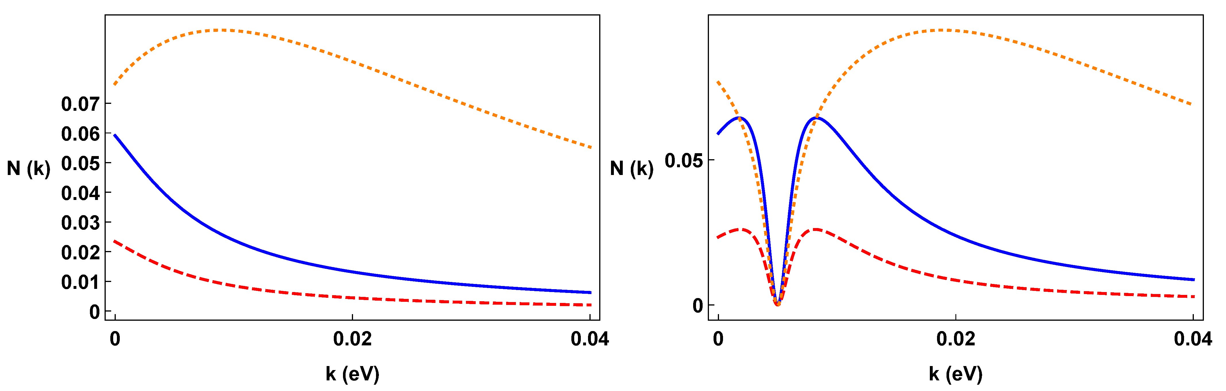
In the case of linearly time-dependent torsion, the violation and the condensation densities are plotted in Figure 9 and Figure 10, respectively, for the same values of the parameters used for Figure 4, Figure 5 and Figure 6.
It is worth noting that the well shape appearing in the right panel of Figure 10 is due to the proportionality of to (see Equation (22)), so that it vanishes for , also bringing the condensation density to zero. english
6. Conclusions
We analyzed the Einstein–Cartan theory and by studying the neutrino propagation on a torsion background in the QFT framework. We derived new oscillation formulae which are dependent on the spin orientations of the neutrino fields. Indeed, we showed that the energy splitting induced by the torsion term affects the oscillation frequencies and the Bogoliubov coefficients which represent the amplitudes of the oscillation formulae. We considered flat space-time and two different kinds of torsion terms, the constant, and the linearly time-dependent torsion.
The two analyzed cases share the following behavior: the spin dependence of the oscillation is maximal for values of torsion comparable to the neutrino momentum and masses, while much larger values of torsion lead to flavor oscillations which are almost independent from the spin. Moreover, a large enough torsion can effectively inhibit the flavor oscillations. Such behaviors also characterize the asymmetry.
The torsion effects are relevant on neutrino oscillations in non-relativistic regimes. Therefore, experiments studying neutrinos with very low momenta, such as PTOLEMY, could provide verification of such results in the future.
Author Contributions
All the authors contributed equally to conceptualization, methodology and writing–original draft preparation. All authors have read and agreed to the published version of the manuscript.
Funding
Partial financial support from MUR and INFN is acknowledged. A.C. also acknowledges the COST Action CA1511 Cosmology and Astrophysics Network for Theoretical Advances and Training Actions (CANTATA).
Data Availability Statement
The data presented in this study are available in the article.
Conflicts of Interest
The authors declare no conflict of interest.
Appendix A. Useful Formulae
For reader convenience, we report formulae useful for the computations. We consider the PNMS matrix. Then, denoting with , the flavor fields and with the fields with definite masses, the mixing relations are
Here, and is the Dirac -violating phase.
The mixing generator is given by where
with free field solutions of Dirac equations with torsion terms.
Bogoliubov coefficients and satisfy the following identities:
Appendix B. Charges for Three Flavor Mixing with Torsion
Charges are introduced using the symmetries of the Lagrangian for free field operators: . The Lagrangian is invariant under global transformation of phase factor of the type . Then, a charge is introduced via Noether’s theorem: ; it represents the total charge of the system. Considering field transformation under global transformation , we obtain Noether charges of the form with and , the time component of currents. The charges satisfy algebra: Note that only charges and , which are not time-dependent. Appropriate combinations of these charges allow to define the following quantities: and The normal ordering of charge operators for free fields are, then,
with where is used to denote the normal ordered with respect to vacuum state . The flavor charges can be directly derived from the above Noether charges by applying the mixing generator to them:
with .
In terms of the flavour annihilators, we have
where is normal-ordered with respect to the vacuum state, indicating .
Note that flavor charge can be written as the sum of the charges for definite spin orientation as
where . The neutrino oscillation formula at fixed momentum and spin are obtained in the Heisenberg picture by computing the following expectation values:
Similarly, for the antiparticle,
Similar formulae are obtained for spin down.
[custom]
| 1 | In the ultrarelativistic case (), one has:
|
References
- Capozziello, S.; Laurentis, M.D. Extended theory of gravity. Phys. Rep. 2011, 509, 167–321. [Google Scholar] [CrossRef]
- Heisenberg, L. Review on f(Q) gravity. Phys. Rep. 2024, 1066, 1–78. [Google Scholar] [CrossRef]
- Anagnostopoulos, F.K.; Basilakos, S.; Saridakis, E.N. First evidence that non-metricity f(Q) gravity could challenge ΛCDM. Phys. Lett. B 2021, 822, 136634. [Google Scholar] [CrossRef]
- Capozziello, S.; D’Agostino, R. Model-independent reconstruction of f(Q), non-metric gravity. Phys. Lett. B 2022, 832, 137229. [Google Scholar] [CrossRef]
- Lin, R.H.; Zhai, X.H. Spherically symmetric configuration in f(Q) gravity. Phys. Rev. D 2021, 103, 124001. [Google Scholar] [CrossRef]
- Xu, Y.; Li, G.; Liang, S.D. f(Q,T) gravity. Eur. Phys. J. C 2019, 79, 708. [Google Scholar] [CrossRef]
- Shankaranarayanan, S.; Johnson, J.P. Modified theories of gravity: Why, how and what? Gen. Relativ. Gravit. 2022, 44, 54. [Google Scholar] [CrossRef]
- Bamba, K.; Capozziello, S.; Nojiri, S.I.; Odintsov, S.D. Dark energy cosmology: The equivalent description via different theoretical models and cosmography tests. Astrophys. Sace Sci. 2012, 342, 155–228. [Google Scholar] [CrossRef]
- Khyllep, W.; Dutta, J.; Saridakis, E.N.; Yesmakhanova, K. Cosmology in f(Q) gravity: A unified dynamical systems analysis of the background and perturbations. Phys. Rev. D 2023, 107, 044022. [Google Scholar] [CrossRef]
- Berti, E.; Barausse, E.; Cardoso, V.; Gualtieri, L.; Pani, P.; Sperhake, U.; Stein, L.C.; Wex, N.; Yagi, K.; Baker, T.; et al. Testing general relativity with present and future astrophysical observations. Class. Quantum Grav. 2015, 32, 243001. [Google Scholar] [CrossRef]
- Sebastiani, L.; Vagnozzi, S.; Myrzakulov, R. Mimetic Gravity: A review of recent developments and applications to cosmology and astrophysics. Adv. High Energy Phys. 2017, 2017, 3156915. [Google Scholar] [CrossRef]
- Rubin, V.C.; Ford, W.K.; Thonnard, N. Rotational properties of 21 SC galaxies with a large range of luminosities from NGC 4605(r = 4kpc) to UGC 2885(R = 122 kpc). Astrophys. J. 1980, 238, 471–487. [Google Scholar] [CrossRef]
- Salucci, P. The distribution of dark matter in galaxies. Astron. Astro. Phys. Rev. 2019, 27, 2. [Google Scholar] [CrossRef]
- Freese, K. Status of dark matter in the universe. Int. J. Mod. Phys. D 2017, 26, 1730012. [Google Scholar] [CrossRef]
- Valentino, E.D.; Melchiorri, A.; Mena, O.; Vignozzi, S. Nonminimal dark sector physics and cosmological tension. Phys. Rev D 2020, 101, 6. [Google Scholar] [CrossRef]
- Rubin, V. Dark matter in spiral galaxies. Sci. Am. 1983, 248, 6. [Google Scholar] [CrossRef]
- Rubin, V., W. K. Ford, Rotation of the Andromeda Nebula from a Spectroscopic survey of emission regions. Astrophys. J. 1970, 159, 379. [Google Scholar] [CrossRef]
- Garret, K.; Duda, G. Dark matter: A primer. Advandes Astron. 2010, 2011, 968283. [Google Scholar] [CrossRef]
- Smith, P.F.; Lewin, J.D. Dark matter detection. Phys. Rep. 1990, 187, 5. [Google Scholar] [CrossRef]
- Hutten, M.; Kerszberg, D. TeV Dark Matter Searches in the Extragalactic Gamma-ray. Galaxies 2022, 10, 5. [Google Scholar] [CrossRef]
- Perivolaropoulos, L.; Skara, F. Challenges for ΛCDM: An update. New Astron. Rev. 2022, 95, 101659. [Google Scholar]
- Fruscianti, N.; Perenon, L. Effective field theory of dark energy: A review. Phys. Rep. 2020, 857, 1–63. [Google Scholar] [CrossRef]
- Oks, E. Brief review of recent advances in undestanding dark matter and dark energy. New Astron. Rev. 2021, 93, 101632. [Google Scholar] [CrossRef]
- Lonappan, A.I.; Kumar, S.; Dinda, B.R.; Sen, A.A. Bayesian evidences for dark energy models in light of current observational data. Phys. Rev. 2018, 97, 4. [Google Scholar] [CrossRef]
- Steinhardt, P.J.; Turok, N. Why the cosmological constant is small and positive. Science 2006, 312, 1180–1183. [Google Scholar] [CrossRef]
- Mehrabi, A.; Basilakos, S. Dark energy reconstruction based on the Padé approximation: An expansion around the ΛCDM. Eur. Phys. J. C 2018, 78, 889. [Google Scholar] [CrossRef]
- Brans, C.; Dicke, R.H. Mach’s principle and a Relativistic Theory of Gravitation. Phys. Rev. 1961, 124, n925. [Google Scholar] [CrossRef]
- Quiros, I. Selected topics in scalar-tensor theories and beyond. Int. J. Mod. Phys. D 2019, 28, 1930012. [Google Scholar] [CrossRef]
- Kobayashi, T. Horndeski theory and beyond: A review. Rep. Prog. Phys. 2019, 82, 086901. [Google Scholar] [CrossRef] [PubMed]
- Capozziello, S.; Cardone, V.F.; Carloni, S.; Troisi, A. Can higher order curvature theories explain rotation curves of galaxies? Phys. Lett. A 2004, 326, 292–296. [Google Scholar] [CrossRef]
- Capozziello, S.; Cardone, V.F.; Carloni, S.; Troisi, A. Higher order curvature theories of gravity matchet with observations: A bridge between dark energy and dark matter problems. Aip Conf. Proc. 2005, 751, 54–63. [Google Scholar]
- Cherubini, C.; Bini, D.; Capozziello, S.; Ruffini, R. Second order scalar invariants of the Riemann tensor: Applications to black hole spacetimes. Int. J. Mod. Phys. D 2002, 11, 827–841. [Google Scholar] [CrossRef]
- Hehl, F.W.; Von der Heyde, P.; Kerlick, G.D. General relativity with spin and torsion: Foundations and prospects. Rev. Mod. Phys. 1976, 48, 393. [Google Scholar] [CrossRef]
- Shapiro, I.L. Physical aspects of the space-time torsion. Phys. Rep. 2002, 357, 113–213. [Google Scholar] [CrossRef]
- Mavromatos, N.E.; Pais, P.; Iorio, A. Torsion at different scale: From materials to the universe. Universe 2023, 9, 516. [Google Scholar] [CrossRef]
- Capozziello, S.; Cianci, R.; Stornaiolo, C.; Vignolo, S. f(R) gravity with torsion: The metric-affine approach. Class. Quantum Gravity 2007, 24, 6417. [Google Scholar] [CrossRef]
- Capozziello, S.; Cianci, R.; Stornaiolo, C.; Vignolo, S. f(R) cosmology with torsion. Phys. Scr. 2008, 78, 065010. [Google Scholar] [CrossRef]
- Vignolo, S.; Fabbri, L.; Cianci, R. Dirac spinors in Bianchi-I f(R)- cosmology with torsion. J. Math. Phys. 2011, 52, 112502. [Google Scholar] [CrossRef]
- Capozziello, S.; Vignolo, S. Metric-affine f(R)- gravity with torsion: An overview. Ann. Der Phys. 2010, 522, 238–248. [Google Scholar] [CrossRef]
- Fabbri, L.; Vignolo, S. A modified theroy of gravity with torsion and its applications to cosmology and particle physics. Int. J. Theor. Phys. 2010, 51, 3186. [Google Scholar] [CrossRef]
- Fabbri, L.; Vignolo, S. Dirac fields in f(R) gravity with torsion. Class. Quantum Gravity 2011, 28, 125002. [Google Scholar] [CrossRef]
- Fabbri, L.; Vignolo, S. ELKO and Dirac Spinors seen from Torsion. Int. J. Mod. Phys. D 2014, 23, 1444001. [Google Scholar] [CrossRef]
- Vignolo, S.; Fabbri, L.; Stornaiolo, C. A square-torsion modification of Einstein-Cartan theory. Ann. Der Phys. 2012, 524, 826–839. [Google Scholar] [CrossRef]
- Fabbri, L.; Vignolo, S.; Carloni, S. Renormalizability of the Dirac equation in torsion gravity with nonminimal coupling. Phys. Rev. D 2014, 90, 024012. [Google Scholar] [CrossRef]
- van de Venn, A.; Vasak, D.; Kirsch, J.; Struckmeier, J. Torsional dark energy in quadratic gauge gravity. Eur. Phys. J. C 2023, 83, 288. [Google Scholar] [CrossRef]
- Cabral, F.; Lobo, F.; Rubiera-Garcia, D. Imprints from a Riemann-Cartan space-time on the energy levels of Dirac spinors. Class. Quantum Grav. 2021, 38, 195008. [Google Scholar] [CrossRef]
- Cirilo-Lombardo, D.J. Fermion helicity flip and fermion oscillation induced by dynamical torsion field. EPL 2019, 127, 10002. [Google Scholar] [CrossRef]
- Aartsen, M. et al. [IceCube Collaboration] Neutrino emission from the direction of the Blazar TXS 0506+ 056 prior to the IceCube-170922A alert. Science 2018, 361, 6398. [Google Scholar]
- Aartsen, M. et al. [The IceCube et al.] Multimessenger observations of a flaring blazar coincident with high-energy neutrino IceCube-170922A. Science 2018, 361, eaat1378. [Google Scholar] [CrossRef] [PubMed]
- Abbasi, R. et al. [ICECUBE Collaboration] Search for Continuous and Transient Neutrino Emission Associated with IceCube’s Highest-Energy Tracks: An 11-Year Analysis. Astrophys. J. 2024, 964, 40. [Google Scholar] [CrossRef]
- Abbasi, R. et al. [ICECUBE Collaboration] Search for 10-1000 GeV Neutrinos from Gamma Ray Bursts with IceCube. Astrophys. J. 2024, 964, 126. [Google Scholar] [CrossRef]
- Abbasi, R. et al. [ICECUBE Collaboration] Search for Neutrino Lines from Dark Matter Annihilation and Decay with IceCube. Phys. Rev. D 2023, 108, 102004. [Google Scholar] [CrossRef]
- Abbasi, R. et al. [ICECUBE Collaboration] Search for Extended Sources of Neutrino Emission in the Galactic Plane with IceCube. Astrophys. J. 2023, 956, 20. [Google Scholar] [CrossRef]
- Abbasi, R. et al. [ICECUBE Collaboration] Searches for Connections between Dark Matter and High-Energy Neutrinos with IceCube. J. Cosmol. Astrophys. Phys. 2023, 10, 3. [Google Scholar]
- Abbasi, R. et al. [ICECUBE Collaboration] Search for Correlations of High-Energy Neutrinos Detected in IceCube with Radio-Bright AGN and Gamma-Ray Emission from Blazars. Astrophys. J. 2023, 954, 75. [Google Scholar] [CrossRef]
- Abbasi, R. et al. [ICECUBE Collaboration] Observation of Seasonal Variations of the Flux of High-Energy Atmospheric Neutrinos with IceCube. Eur. Phys. J. C 2023, 83, 777. [Google Scholar] [CrossRef]
- Abbasi, R. et al. [ICECUBE Collaboration] Search for sub-TeV Neutrino Emission from Novae with IceCube-DeepCore. Astrophys. J. 2023, 953, 160. [Google Scholar] [CrossRef]
- Abud, A.A. et al. [DUNE Collaboration] Impact of cross-section uncertainties on supernova neutrino spectral parameter fitting in the deep underground neutrino experiment. Phys. Rev. D 2023, 107, 112012. [Google Scholar] [CrossRef]
- Abud, A. A. et al. [DUNE Collaboration] Low exposure long-baseline neutrno oscillation sensitivity of the DUNE experiment. Phys. Rev. D 2022, 105, 072006. [Google Scholar] [CrossRef]
- Abi, B. et al. [DUNE Collaboration] Prospects for beyond the prospects for beyond the standard model physics searches at the Deep Underground Neutrino Experiment. Eur. Phys. J. C 2021, 81, 322. [Google Scholar] [CrossRef] [PubMed]
- Sabelnikov, A.; Santin, G.; Skorokhvatov, M.; Sobel, H.; Steele, J.; Steinberg, R.; Sukhotin, S.; Tomshaw, S.; Veron, D.; Vyrodov, V.; et al. Search for neutrino oscillations on a long base-line at the CHOOZ nuclear power station. Eur. Phys. J. C 2003, 27, 331–374. [Google Scholar]
- Abdurashitov, J.N.; Gavrin, V.N.; Girin, S.V.; Gorbachev, V.V.; Ibragimova, T.V.; Kalikhov, A.V.; Khairnasov, N.G.; Knodel, T.V.; Mirmov, I.N.; Shikhin, A.A.; et al. Measurement of the solar neutrino capture rate with gallium metal. Phys. Rev. C 1999, 60, 055801. [Google Scholar] [CrossRef]
- Adamson, P.; Aliaga, L.; Ambrose, D.; Anfimov, N.; Antoshkin, A.; Arrieta-Diaz, E.; Augsten, K.; Aurisano, A.; Backhouse, C.; Baird, M.; et al. Search for active-sterile neutrino mixing using neutral-current interactions in NOvA. Phys. Rev. D 2017, 96, 072006. [Google Scholar] [CrossRef]
- Buchmüller, W. Neutrino, Grand Unification and Leptogenesis. arXiv, 2004; arXiv:hep-ph/0204288. [Google Scholar]
- Capolupo, A.; Carloni, S.; Quaranta, A. Quantum flavor vacuum in the expanding universe: A possible candidate for cosmological dark matter? Phys. Rev. D 2022, 105, 105013. [Google Scholar] [CrossRef]
- Capolupo, A.; Giampaolo, S.M.; Lambiase, G.; Quaranta, A. Probing quantum field theory particle mixing and dark-matter-like effects with Rydberg atoms. EPJ C 2020, 80, 423. [Google Scholar] [CrossRef]
- Kaplan, D.B.; Nelson, A.E.; Weiner, N. Neutrino Oscillation as a probe of Dark Energy. Phys. Rev. Lett. 2004, 93, 091801. [Google Scholar] [CrossRef] [PubMed]
- Bilenky, S.M.; Pontecorvo, B. Lepton mixing and neutrino oscillations. Phys. Rep. 1978, 41, 225. [Google Scholar] [CrossRef]
- Bilenky, S.M.; Petcov, S.T. Massive neutrinos and neutrino oscillations. Rev. Mod. Phys. 1987, 59, 671. [Google Scholar] [CrossRef]
- Aad, G. et al. [ATLAS Collaboration] Observation of a new particle in the search for the standard Model Higgs boson with the ATLAS detector at the LHC. Phys. Lett. B 2012, 716, 1–29. [Google Scholar] [CrossRef]
- Fukuda, Y.; Hayakawa, T.; Ichihara, E.; Inoue, K.; Ishihara, K.; Ishino, H.; Itow, Y.; Kajita, T.; Kameda, J.; Kasuga, S.; et al. Evidence for Oscillation of Atmospheric Neutrinos. Phys. Rev. Lett. 1998, 81, 1562–1567. [Google Scholar] [CrossRef]
- Blasone, M.; Vitiello, G. Quantum Field Theory of Fermion Mixing. Ann. Phys. 1995, 244, 283–311. [Google Scholar] [CrossRef]
- Blasone, M.; Capolupo, A.; Vitiello, G. Quantum field theory of three flavor neutrino mixing and oscillations with CP violation. Phys. Rev. D 2002, 66, 025033. [Google Scholar] [CrossRef]
- Capolupo, A.; Capozziello, S.; Vitiello, G. Neutrino mixing as a source of dark energy. Phys. Lett. A 2007, 363, 53. [Google Scholar] [CrossRef]
- Capolupo, A. Dark matter and dark energy induced by condensates. Adv. High Energy Phys. 2016, 2016, 8089142. [Google Scholar] [CrossRef]
- Capolupo, A. Quantum vacuum, dark matter, dark energy and spontaneous supersymmetry breaking. Adv. High Energy Phys. 2018, 2018, 9840351. [Google Scholar] [CrossRef]
- Fujii, K.; Habe, C.; Yabuki, T. Note on the field theory of neutrino mixing. Phys. Rev. D 1999, 59, 113003. [Google Scholar] [CrossRef]
- Hannabuss, K.C.; Latimer, D.C. The quantum field theory of fermion mixing. J. Phys. A 2000, 33, 1369. [Google Scholar] [CrossRef]
- Blasone, M.; Capolupo, A.; Romei, O.; Vitiello, G. Quantum field theory of boson mixing. Phys. Rev. D 2001, 63, 125015. [Google Scholar] [CrossRef]
- Alfinito, E.; Blasone, M.; Iorio, A.; Vitiello, G. Squeezed neutrino Oscillations in Quantum Field Theory. Phys. Lett. B 1995, 362, 91. [Google Scholar] [CrossRef]
- Grossman, Y.; Lipkin, H.J. Flavor oscillations from a spatially localized source: A simple general treatment. Phys. Rev. D 1997, 55, 2760. [Google Scholar] [CrossRef]
- Piriz, D.; Roy, M.; Wudka, J. Neutrino oscillations in strong gravitational fields. Phys. Rev. D 1996, 54, 1587. [Google Scholar] [CrossRef] [PubMed]
- Cardall, C.Y.; Fuller, G.M. Neutrino oscillations in curved spacetime: A heuristic treatment. Phys. Rev. D 1997, 55, 7960. [Google Scholar] [CrossRef]
- Buoninfante, L.; Luciano, G.G.; Petruzziello, L.; Smaldone, L. Neutrino oscillations in extended theories of gravity. Phys. Rev. D 2020, 101, 024016. [Google Scholar] [CrossRef]
- Capolupo, A.; Giampaolo, S.M.; Quaranta, A. Geometric phase of neutrinos: Differences between Dirac and Majorana neutrinos. Phys. Lett. B 2021, 820, 136489. [Google Scholar] [CrossRef]
- Luciano, G.G. On the flavor/mass dichotomy for mixed neutrinos: A phenomenologically motivated analysis based on lepton charge conservation in neutron decay. EPJ Plus 2023, 138, 83. [Google Scholar] [CrossRef]
- Capolupo, A.; Quaranta, A. Neutrinos, mixed bosons, quantum reference frames and entanglement. J. Phys. G 2023, 50, 055003. [Google Scholar] [CrossRef]
- Capolupo, A.; Quaranta, A. neutrino capture on tritium as a probe of flavor vacuum condensate and dark matter. Phys. Lett. B 2023, 839, 137776. [Google Scholar] [CrossRef]
- Bilenky, S.M.; Hošek, J.; Petcov, S.T. On the oscillations of neutrinos with Dirac and Majorana masses. Phys. Lett. B 1980, 94, 495–498. [Google Scholar] [CrossRef]
- Capolupo, A.; Giampaolo, S.M.; Hiesmayr, B.C.; Lambiase, G.; Quaranta, A. On the geometric phase for Majorana and Dirac neutrinos. J. Phys. G 2023, 50, 025001. [Google Scholar] [CrossRef]
- Fogli, G.L.; Lisi, E.; Marrone, A.; Montanino, D.; Palazzo, A. Global analysis of three-flavor neutrino masses and mixing. Prog. Part. Nucl. Phys. 2006, 57, 742–795. [Google Scholar] [CrossRef]
- Capozzi, F.; Valentino, E.D.; Lisi, E.; Marrone, A.; Melchiorri, A.; Palazzo, A. Global constraints on absolute neutrino masses and their ordering. Phys. Rev. D 2017, 95, 096014. [Google Scholar] [CrossRef]
- Capozzi, F.; Lisi, E.; Marrone, A.; Montanino, D.; Palazzo, A. Neutrino masses and mixings: Status of known and unknown 3v parameters. Nucl. Phys. B 2016, 908, 218–234. [Google Scholar] [CrossRef]
- Fogli, G.L.; Lisi, E.; Montanino, D.; Palazzo, A. Observables sensitive to absolute neutrino masses. II. Phys. Rev. D 2008, 79, 033010. [Google Scholar] [CrossRef]
- Fogli, G.L.; Lisi, E.; Marrone, A.; Melchiorri, A.; Palazzo, A.; Serra, P.; Silk, J. Observables sensitive to absolute neutrino masses: Constraints and correlations from world neutrino data. Phys. Rev. D 2004, 70, 113003. [Google Scholar] [CrossRef]
- Fogli, G.L.; Lisi, E.; Marrone, A.; Melchiorri, A.; Palazzo, A.; Serra, P.; Silk, J.; Slosar, A. Observables sensitive to absolute neutrino masses: A reappraisal after WMAP 3-year and first MINOS results. Phys. Rev. D 2007, 75, 053001. [Google Scholar] [CrossRef]
- Adak, M.; Dereli, T.; Ryder, H. Neutrino Oscillations Induced by Space-Time Torsion. Class. Quantum Grav. 2001, 18, 1503–1512. [Google Scholar] [CrossRef]
- Fabbri, L.; Vignolo, S. A torsional completion of gravity for Dirac matter fields and its applications to neutrino oscillations. Mod. Phys. Lett. A 2016, 31, 1650014. [Google Scholar] [CrossRef]
- Betti, M.G. et al. [PTOLEMY Collaboration] Neutrino physics with the PTOLEMY project: Active neutrino properties and the light sterile case. JCAP 2019, 2019, 47. [Google Scholar] [CrossRef]
- Kapusta, J.I. Neutrino superfluidity. Phys. Rev. Lett. 2004, 93, 251801. [Google Scholar] [CrossRef]
- Capolupo, A.; Lambiase, G.; Quaranta, A. Neutrinos in curved spacetime: Particle mixing and flavor oscillations. Phys. Rev. D 2020, 101, 095022. [Google Scholar] [CrossRef]
- Capolupo, A.; Lambiase, G.; Quaranta, A. Fermion mixing in curved spacetime. J. Phys. Conf. Ser. 2023, 2533, 012050. [Google Scholar] [CrossRef]
- Capolupo, A.; Quaranta, A.; Serao, R. Field Mixing in Curved Spacetime and Dark Matter. Symmetry 2023, 15, 807. [Google Scholar] [CrossRef]
- Capolupo, A.; Quaranta, A.; Setaro, P.A. Boson mixing and flavor oscillations in curved spacetime. Phys. Rev. D 2022, 106, 043013. [Google Scholar] [CrossRef]
- Capolupo, A.; Quaranta, A. Boson mixing and flavor vacuum in the expanding Universe: A possible candidate for the dark energy. Phys. Lett. B 2023, 840, 137889. [Google Scholar] [CrossRef]
- Blasone, M.; Lambiase, G.; Luciano, G.G.; Petruzziello, L.; Smaldone, L. Time-energy uncertainty relation for neutrino oscillation curved spacetime. Quantum Grav. 2020, 37, 155004. [Google Scholar] [CrossRef]
- Abi, B.; Acciarri, R.; Acero, M.A.; Adamov, G.; Adams, D.; Adinolfi, M.; Ahmad, Z.; Ahmed, J.; Alion, T.; Alonso Monsalve, S.; et al. Supernova neutrino burst detection with the Deep underground neutrino Experiment. EPJ 2021, 81, 423. [Google Scholar] [CrossRef]
- Abi, B.; Acciarri, R.; Acero, M.A.; Adamov, G.; Adams, D.; Adinolfi, M.; Ahmad, Z.; Ahmed, J.; Alion, T.; Monsalve, S.A.; et al. Long-baseline neutrino oscillation physics potential of the DUNE experiment. EPJ 2020, 80, 978. [Google Scholar] [CrossRef]
Figure 1.
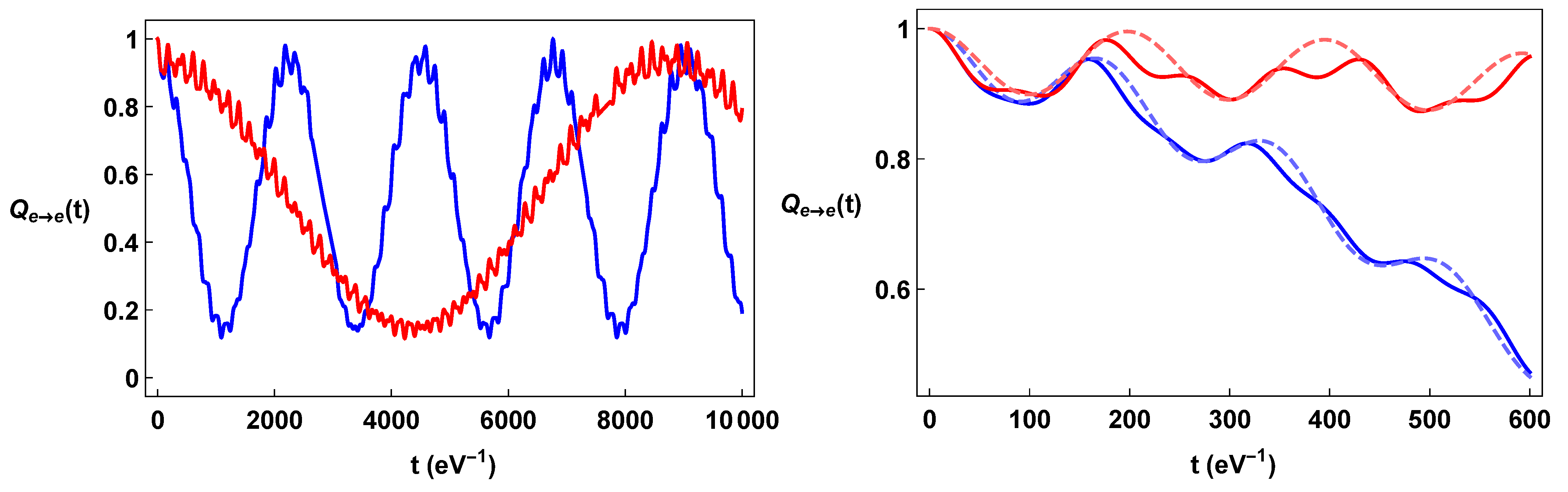
Color on line. Plots of the oscillation formulae in a constant torsion background: in the left-hand panel (blue line) and (red line) as a function of time. Torsion was picked to be comparable to the momentum as . In the right panel, the detail of the same formulae and the comparison with the corresponding quantum mechanics oscillation formulae (dashed line) are reported.
Figure 1.
Color on line. Plots of the oscillation formulae in a constant torsion background: in the left-hand panel (blue line) and (red line) as a function of time. Torsion was picked to be comparable to the momentum as . In the right panel, the detail of the same formulae and the comparison with the corresponding quantum mechanics oscillation formulae (dashed line) are reported.

Figure 2.
Color on line. In the left-hand panel, plots of (blue line) and (red line) as a function of time. In the right panel, details of the same formulae and comparison with the corresponding QM oscillation formulae (dashed line).
Figure 2.
Color on line. In the left-hand panel, plots of (blue line) and (red line) as a function of time. In the right panel, details of the same formulae and comparison with the corresponding QM oscillation formulae (dashed line).
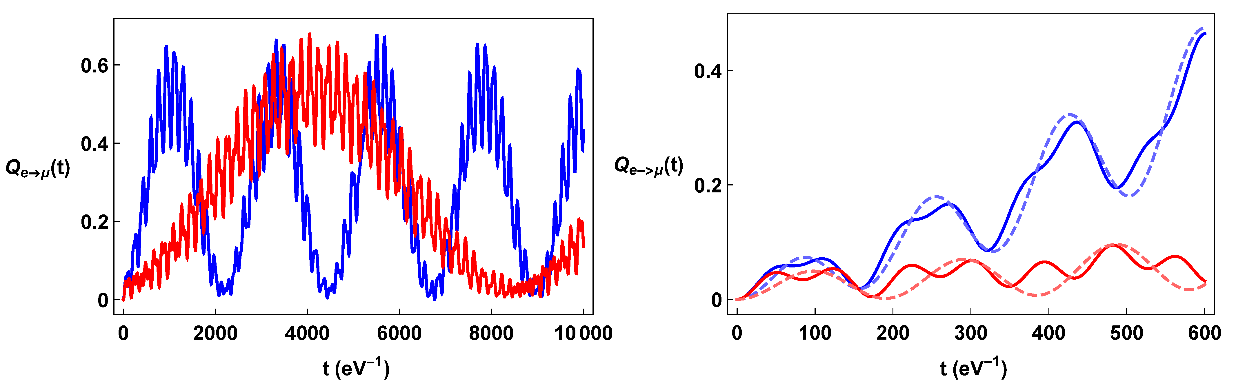
Figure 3.
Color on line. In the left-hand panel, plots of (blue line) and (red line) as a function of time. In the right panel, details of the same formulae and comparison with the corresponding QM formulae (dashed line).
Figure 3.
Color on line. In the left-hand panel, plots of (blue line) and (red line) as a function of time. In the right panel, details of the same formulae and comparison with the corresponding QM formulae (dashed line).
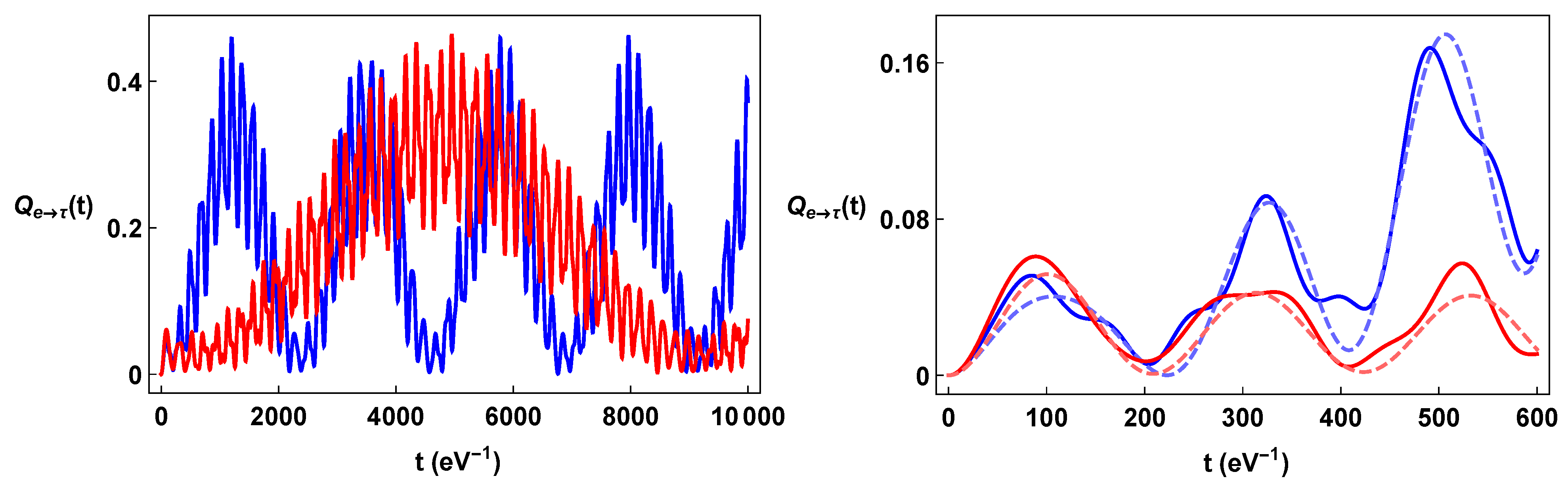
Figure 4.
Color on line. Plots of the oscillation formulae in a time-dependent torsion: in the left-hand panel, (blue line) and (red line) are plotted as a function of time. In the right panel, the details of the same formulae and the comparison with the corresponding quantum mechanics oscillation formulae (dashed line) are reported. We consider .
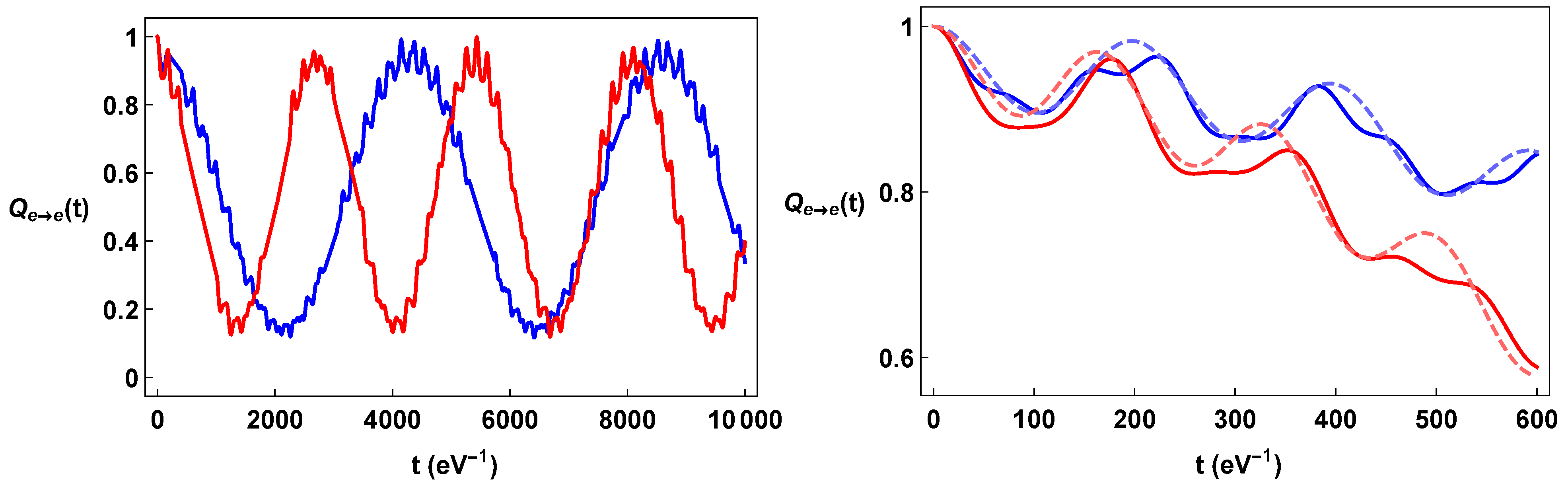
Figure 5.
Color online. In the left-hand panel, (blue line) and (red line) ae plotted as a function of time. In the right panel, the details of the same formulae and the comparison with the corresponding QM formulae (dashed line) are presented.
Figure 5.
Color online. In the left-hand panel, (blue line) and (red line) ae plotted as a function of time. In the right panel, the details of the same formulae and the comparison with the corresponding QM formulae (dashed line) are presented.

Figure 6.
Color online. In the left-hand panel, (blue line) and (red line) are plotted as a function of time. In the right panel, the details of the same formulae and the comparison with the corresponding QM formulae (dashed line) are reported.
Figure 6.
Color online. In the left-hand panel, (blue line) and (red line) are plotted as a function of time. In the right panel, the details of the same formulae and the comparison with the corresponding QM formulae (dashed line) are reported.
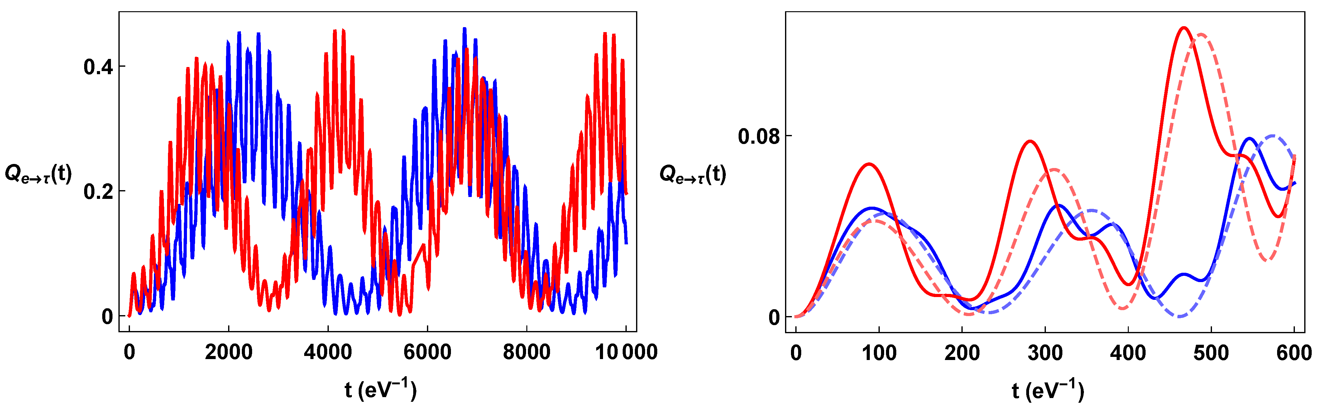
Figure 7.
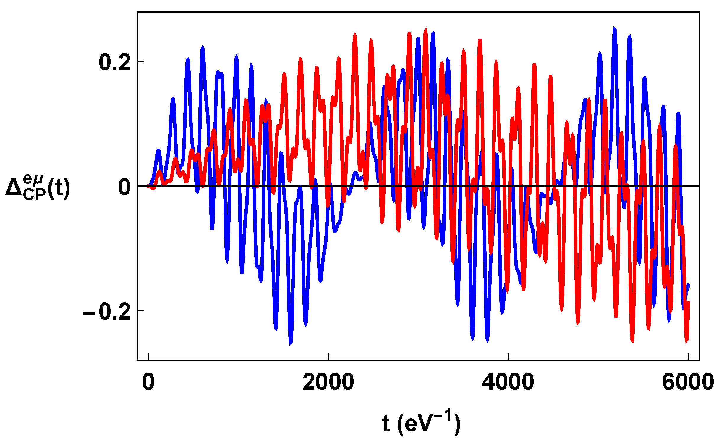
Color on line. Plot of (blue line) and (red line) as a function of time for the values of the parameters used in Figure 1, Figure 2 and Figure 3.

Figure 8.
Color online. (Left panel) Plots of as a function of in : (blue solid), (red dashed line) and (orange dotted line). (Right panel) Plots of as a function of . We use the same parameters as adopted in Figure 1, Figure 2 and Figure 3.
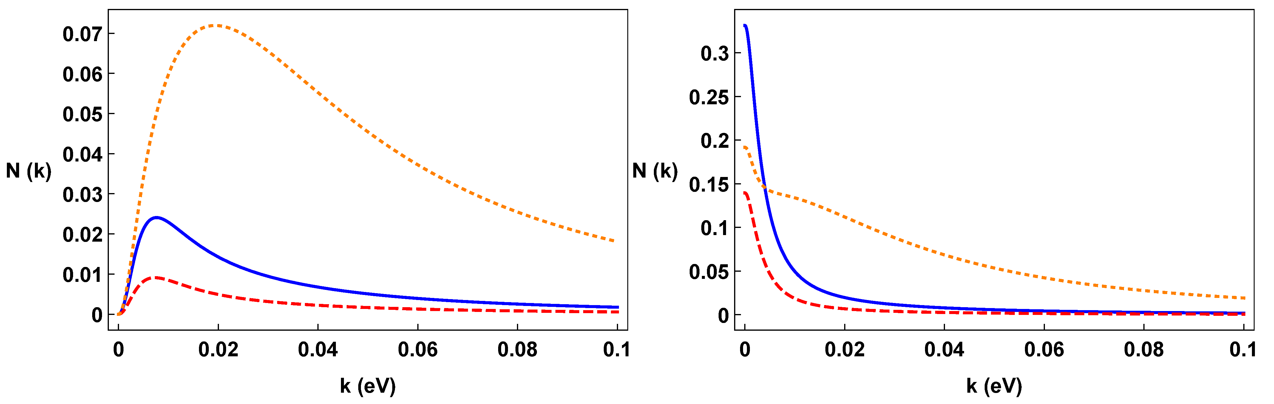
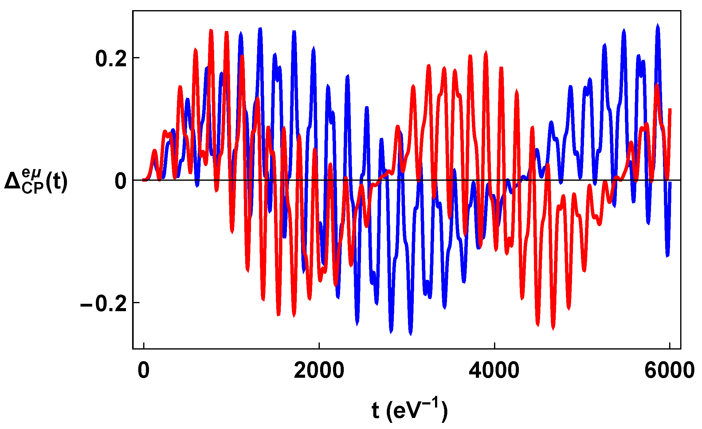
Figure 9.
Color on line. Plot of (blue) (red) as a function of time for the same parameters used in Figure 4, Figure 5 and Figure 6.

Disclaimer/Publisher’s Note: The statements, opinions and data contained in all publications are solely those of the individual author(s) and contributor(s) and not of MDPI and/or the editor(s). MDPI and/or the editor(s) disclaim responsibility for any injury to people or property resulting from any ideas, methods, instructions or products referred to in the content. |
© 2024 by the authors. Licensee MDPI, Basel, Switzerland. This article is an open access article distributed under the terms and conditions of the Creative Commons Attribution (CC BY) license (https://creativecommons.org/licenses/by/4.0/).
Share and Cite
MDPI and ACS Style
Capolupo, A.; De Maria, G.; Monda, S.; Quaranta, A.; Serao, R. Quantum Field Theory of Neutrino Mixing in Spacetimes with Torsion. Universe 2024, 10, 170. https://doi.org/10.3390/universe10040170
AMA Style
Capolupo A, De Maria G, Monda S, Quaranta A, Serao R. Quantum Field Theory of Neutrino Mixing in Spacetimes with Torsion. Universe. 2024; 10(4):170. https://doi.org/10.3390/universe10040170
Chicago/Turabian StyleCapolupo, Antonio, Giuseppe De Maria, Simone Monda, Aniello Quaranta, and Raoul Serao. 2024. "Quantum Field Theory of Neutrino Mixing in Spacetimes with Torsion" Universe 10, no. 4: 170. https://doi.org/10.3390/universe10040170
Note that from the first issue of 2016, this journal uses article numbers instead of page numbers. See further details here.