A Note on Rectangular Partially Massless Fields

Abstract

We study a class of non-unitary $\mathfrak{so}(2,d)$ representations (for even values of d), describing mixed-symmetry partially massless fields which constitute natural candidates for defining higher-spin singletons of higher order. It is shown that this class of $\mathfrak{so}(2,d)$ modules obeys of natural generalisation of a couple of defining properties of unitary higher-spin singletons. In particular, we find out that upon restriction to the subalgebra $\mathfrak{so}(2,d-1)$, these representations branch onto a sum of modules describing partially massless fields of various depths. Finally, their tensor product is worked out in the particular case of $d=4$, where the appearance of a variety of mixed-symmetry partially massless fields in this decomposition is observed.

Contents

1	Introduction	2
2	Notation and Conventions	4
3	Higher-Order Higher-Spin Singletons	6
	3.1 Unitary Higher-Spin Singletons . . . . . . . . . . . . . . . . . . . . . . . . . . . . . . . . . . . . . . . . . . . . . . . . . . . . . . . . . . . . . . . . . . . . . . . . .	6
	3.2 Non-Unitary, Higher-Order Extension . . . . . . . . . . . . . . . . . . . . . . . . . . . . . . . . . . . . . . . . . . . . . . . . . . . . . . . . . . . . . . . . . . .	12
	3.3 Candidates for Higher-Spin Higher-Order Singletons . . . . . . . . . . . . . . . . . . . . . . . . . . . . . . . . . . . . . . . . . . . . . . . . . . . . . .	15
4	Flato-Frønsdal Theorem	20
5	Conclusions	22
A	Branching Rules and Tensor Products of $\mathfrak{so}\mathbf{(}\mathit{d}\mathbf{)}$	22
	A.1 Branching Rules for $\mathfrak{so}(d)$ . . . . . . . . . . . . . . . . . . . . . . . . . . . . . . . . . . . . . . . . . . . . . . . . . . . . . . . . . . . . . . . . . . . . . . . . . . . . .	22
	A.2 Computing $\mathfrak{so}(d)$ Tensor Products . . . . . . . . . . . . . . . . . . . . . . . . . . . . . . . . . . . . . . . . . . . . . . . . . . . . . . . . . . . . . . . . . . . . . .	23
B	Technical Proofs	24
	B.1 Proof of the Branching Rule for Unitary HS Singletons . . . . . . . . . . . . . . . . . . . . . . . . . . . . . . . . . . . . . . . . . . . . . . . . . . . . .	24
	B.2 Proof of the Branching Rule for Rectangular Partially Massless Fields . . . . . . . . . . . . . . . . . . . . . . . . . . . . . . . . . . . . . . . . .	27
References		32

1. Introduction

The completion of the Bargmann-Wigner program in anti-de Sitter (AdS) spacetime 1 lead to some surprising lessons concerning the definition of masslessness in other backgrounds than Minkowski space. If nowadays, the most common way to discriminate between massless and massive fields in AdS is whether or not they enjoy some gauge symmetry, other proposals which involve a particular kind of $\mathfrak{so}(2,d)$ representations known as “singletons”, were put forward [4,5]. Indeed, the proposed notions of “conformal masslessness” and “composite masslessness” both rely on two crucial properties of singletons, namely 2:

• They are unitary and irreducible representations (UIRs) of $\mathfrak{so}(2,d)$ that remain irreducible when restricted to UIRs of $\mathfrak{so}(2,d-1)$, or in other words they correspond to the class of elementary particles in d-dimensional anti-de Sitter space which are conformal. This property is the very definition of a conformally massless UIR, and it turns out that the singletons are precisely the $\mathfrak{so}(2,d)$ UIRs to which conformally massless $\mathfrak{so}(2,d-1)$ UIRs can be lifted.
• The tensor product of two $\mathfrak{so}(2,3)$ singletons contains all conformally massless fields in AdS${}_4$ [7]. In any dimensions however, the representations appearing in the decomposition of the tensor product of two $\mathfrak{so}(2,d)$ singletons (of spin 0 or $\frac{1}{2}$) are no longer conformally massless but make up, by definition, all of the composite massless UIRs of $\mathfrak{so}(2,d)$ [6,8,9,10]. In other words, composite massless UIRs are those modules which appear in the decomposition of the tensor product of two singletons.

This tensor product decomposition, called the Flato-Frønsdal theorem, is crucial in the context of Higher-Spin Gauge Theories and can be summed up as follows (in the case of two scalar singletons):

$$\mathrm{Rac}\otimes \mathrm{Rac}=\mathrm{Massive}\mathrm{scalar}\oplus \underset{s=1}{\overset{\infty }{⨁}}\mathrm{Gauge}\mathrm{field}\mathrm{of}\mathrm{spin}s,$$

(1)

where $\mathrm{Rac}$ denotes the $\mathfrak{so}(2,d)$ scalar singleton. Notice that the spin-$s⩾$ 1 gauge fields are both “composite massless” by definition, as well as massless in the modern sense (as they enjoy some gauge symmetry), whereas the scalar field is considered massive in the sense of being devoid of said gauge symmetries (despite the fact that it is also “composite massless”). The $\mathfrak{so}(2,d)$ UIRs on the right hand side make up the spectrum of fields of Vasiliev’s higher-spin gravity [11,12,13,14] (see e.g., [15,16,17] for, respectively, non-technical and technical reviews). This decomposition can also be interpreted in terms of operators of a free d-dimensional Conformal Field Theory (CFT) as on the left hand side, the tensor product of two scalar singletons can be thought of as a bilinear operator in the fundamental scalar field and the right hand side as the various conserved currents that this CFT possesses. This dual interpretation of Equation (1) is by now regarded as a first evidence in favor of the AdS/CFT correspondence [18,19,20] in the context of Higher-Spin theory [21,22]. This duality relates (the type A) Vasiliev’s bosonic (minimal) higher-spin gravity to the free $U(N)$ ($O(N)$) vector model and has passed several non-trivial checks since it has been proposed, from the computation and matching of the one-loop partition functions [23,24] to three point functions [25,26,27] on both sides of the duality (see e.g., [28,29,30,31] and references therein for reviews of this duality). The possible existence of such an equivalence between the type-A Higher-Spin (HS) theory and the free vector model opened the possibility of probing interactions in the bulk using the knowledge gathered on the CFT side, a program which was tackled in [32] (improving the earlier works [33,34,35]). This lead to the derivation of all cubic vertices and the quartic vertex for four scalar fields in the bulk [36,37], as dictated by the holographic duality, while [38] also raising questions on the locality properties of the bulk HS theory (see e.g., [39,40,41,42,43] and references therein for more details).

The fact that the prospective CFT dual to a HS theory in AdS${}_{d+1}$ is free can be understood retrospectively thanks to the Maldacena-Zhiboedov theorem [44] and its generalisation [45,46]. Indeed, it was shown in [44] that if a 3-dimensional CFT which is unitary, obeys the cluster decomposition axiom and has a (unique) Lorentz covariant stress-tensor plus at least one higher-spin current, then this theory is either a CFT of free scalars or free spinors. This was generalised to arbitrary dimensions in [45,46] 3, where the authors showed that this result holds in dimensions $d⩾3$, up to the additional possibility of a free CFT of $(\frac{d-2}{2})$-forms in even dimensions. These free conformal fields precisely correspond to the singleton representations of spin 0, $\frac{1}{2}$ and 1 in arbitrary dimensions [5,48] 4. Due to the fact that, according to the standard AdS/CFT dictionary, the higher-spin gauge field making up the spectrum of the Higher-Spin theory in the bulk are dual to higher-spin conserved current on the CFT side, this CFT should be free 5 as it falls under the assumption of the previously recalled results of [44,45,46]. Hence, the algebra generated by the set of charges associated with the conserved currents of the CFT whose fundamental field is a spin-s singletons corresponds to the HS algebra of the HS theory in the bulk with a spectrum of field given by the decomposition of the tensor product of two spin-s singletons. These HS algebras can be defined as follows:

$${\mathfrak{hs}}_s^{(d)}\cong \frac{\mathcal{U}\left(\mathfrak{so}(2,d)\right)}{\mathrm{Ann}\left({\mathcal{D}}_s^{\mathrm{sing}.}\right)},$$

(2)

where ${\mathfrak{hs}}_s^{(d)}$ stands for the HS algebra associated with the spin-s singleton in AdS${}_{d+1}$, and $\mathcal{U}\left(\mathfrak{so}(2,d)\right)$ denotes the universal enveloping algebra of $\mathfrak{so}(2,d)$ whereas ${\mathcal{D}}_s^{\mathrm{sing}.}$ denotes the spin-s singleton module of $\mathfrak{so}(2,d)$ and $\mathrm{Ann}\left({\mathcal{D}}_s^{\mathrm{sing}.}\right)$ the annihilator of this module. For more details, see e.g., [6,52,53] where the construction of HS algebras (and their relation with minimal representations of simple Lie algebras [54]) is reviewed and [55] where HS algebras associated with HS singletons were studied. Although Vasiliev’s Higher-Spin theory is based on the HS algebra ${\mathfrak{hs}}_0^{(d)}$ and the HS theory based on ${\mathfrak{hs}}_s^{(d)}$ with $s=\frac{1}{2},1,\dots$, is unknown 6, the latter algebras are quite interesting as they all describe a spectrum containing mixed-symmetry fields. Even though this last class of massless field is well understood at the free level (in flat space as well as in AdS) [56,57,58,59,60,61,62,63,64,65,66,67,68,69,70,71,72,73,74], little is known about their interaction (see e.g., [52,75,76,77,78] on cubic vertices and [79,80,81] where mixed-symmetry fields have been studied in the context of the AdS/CFT correspondence).

A possible extension of the HS algebras associated with singletons can be obtained by applying the above construction (2) with a generalisation of the singleton representations ${\mathcal{D}}_s^{\mathrm{sing}.}$, referred to as “higher-order” singletons. The latter are also irreducible representations of $\mathfrak{so}(2,d)$, which share the property of describing fields “confined” to the boundary of AdS with the usual singletons but which are non-unitary (as detailed in [82]). This class of higher-order singletons, which are of spin 0 or $\frac{1}{2}$, is labelled by a (strictly) positive integer ℓ. In the case of the scalar singleton of order ℓ, such a representation describes a conformal scalar $\varphi$ obeying the polywave equation:

$${\square }^{\ell }\varphi =0.$$

(3)

When $\ell =1$ one recovers the usual singleton (free, unitary conformal scalar field), whereas $\ell >1$ leads to non-unitary CFT. Such CFTs were studied in [83] for instance, and were proposed to be dual to HS theories [82] whose spectrum consists, on top of the infinite tower of (totally symmetric) higher-spin massless fields, also partially massless (totally symmetric) fields of arbitrary spin (theories which have been studied recently in [84,85,86]), thereby extending the HS holography proposal of Klebanov-Polyakov-Sezgin-Sundell to the non-unitary case. The corresponding HS algebras were studied in [87] for the simplest case $\ell =2$ (as the symmetry algebra of the Laplacian square, thereby generalising the previous characterisation of ${\mathfrak{hs}}_0^{(d)}$ as the symmetry algebra of the Laplacian [88]) and for general values of ℓ in [89,90,91]. As we already mentionned, the interesting feature of such HS algebras is that their spectrum, i.e., the set of fields of the bulk theory, contains partially massless (totally symmetric) higher-spin fields [82] (introduced originally in [92,93,94,95], and whose free propagation was described in the unfolded formalism in [96]). Although non-unitary in AdS background, partially massless fields of arbitrary spin are unitary in de Sitter background [97], and hence constitute a particularly interesting generalisation of HS gauge fields to consider 7. Partially massless fields, both totally symmetric and of mixed-symmetry, also appear in the spectrum of the HS algebra based on the order-ℓ spinor singleton [100]. It seems reasonable to expect that the known spectrum of the HS algebras based on a spin-s singleton is enhanced, when considering the HS algebras based on their higher-order extension, with partially massless fields of the same symmetry type as already present in the case of the original singleton. Therefore, a natural question is whether or not there exist higher-order higher-spin singletons. This question is adressed in the present note, in which we study a class of $\mathfrak{so}(2,d)$ modules which is a natural candidate for defining a higher-order higher-spin singleton.

This paper is organised as follows: in Section 2 we start by introducing the various notations that will be used throughout this note, then in Section 3 we first review the defining properties of the well-known (unitary) higher-spin singletons before introducing their would-be higher-order extension and spelling out the counterpart of the previously recalled characteristic properties. Finally, the tensor product of two such representations is decomposed in the low-dimensional case $d=4$ in Section 4. Technical details on the branching and tensor product rule of $\mathfrak{so}(d)$ can be found in Appendix A while details of the proofs of Propositions 2 and 3 and are relegated to Appendix B.

2. Notation and Conventions

In the rest of this paper, we will use the following symbols:

• A $\mathfrak{so}(2,d)$ (generalised Verma) module is characterised by the $\mathfrak{so}(2)\oplus \mathfrak{so}(d)$ lowest weight $[\Delta ;\mathit{\ell }]$, where $\Delta$ is the $\mathfrak{so}(2)$ weight (in general a real number, and more often in this paper, a positive integer) corresponding to the minimal energy of the AdS field described by this representation and ℓ is a dominant integral $\mathfrak{so}(d)$ weight corresponding to the spin of the representation. If irreducible, those modules will be denoted $\mathcal{D}(\Delta ;\mathit{\ell })$, whereas if reducible (or indecomposable), they will be denoted $\mathcal{V}(\Delta ;\mathit{\ell })$.
• The spin $\mathit{\ell }\equiv ({\ell }_1,\dots ,{\ell }_r)$, with $r:=\mathrm{rank}(\mathfrak{so}(d))\equiv [\frac{d}{2}]$ (and where $[x]$ is the integer part of x), is a $\mathfrak{so}(d)$ integral dominant weight. The property that the weight ℓ is integral means that its components ${\ell }_i,i=1,\dots ,r$ are either all integers or all half-integers. The fact that ℓ is dominant means that the components are ordered in decreasing order, and all positive except for the component ${\ell }_r$ when $d=2r$. More precisely,

  $${\ell }_1⩾{\ell }_2⩾\cdots ⩾{\ell }_{r-1}⩾{\ell }_r⩾0,\mathrm{for}\mathfrak{so}(2r+1),$$

  (4)

  and

  $${\ell }_1⩾{\ell }_2⩾\cdots ⩾{\ell }_{r-1}⩾\left|{\ell }_r\right|,\mathrm{for}\mathfrak{so}(2r).$$

  (5)
• In order to deal more efficiently with weight having several identical components, we will use the notation:

  $$(\underset{h_1\mathrm{times}}{\underbrace{{\ell }_1,\dots ,{\ell }_1}},\underset{h_2\mathrm{times}}{\underbrace{{\ell }_2,\dots ,{\ell }_2}},\dots ,\underset{h_k\mathrm{times}}{\underbrace{{\ell }_k,\dots ,{\ell }_k}})\equiv ({\ell }_1^{h_1},{\ell }_2^{h_2},\dots ,{\ell }_k^{h_k}),\mathrm{with}k⩽r,$$

  (6)

  in other words the number h of components with the same value ℓ appears as the exponent of the latter. For the special cases where all components of the highest weight are equal either to 0 or to $\frac{1}{2}$, we will use bold symbols (and forget about the brackets), i.e.,

  $$\mathbf{0}:=(0,\dots ,0),\mathrm{and}\frac{\mathbf{1}}{\mathbf{2}}:=(\frac{1}{2},\dots ,\frac{1}{2}).$$

  (7)

  We will also write only the non-vanishing components of the various $\mathfrak{so}(d)$ weight encountered in this paper, i.e.,

  $$(s_1,\dots ,s_k):=(s_1,\dots ,s_k,\underset{r-k}{\underbrace{0,\dots ,0}}),\mathrm{for}1⩽k⩽r.$$

  (8)
• If the spin is given by an irrep of an even dimensional orthogonal algebra, i.e., $\mathfrak{so}(d)$ for $d=2r$, the last component ${\ell }_r$ of this highest weight (if non-vanishing) can either be positive or negative. Whenever the statements involving such a weight does not depend on this sign, we will write $\mathit{\ell }=({\ell }_1,\dots ,{\ell }_r)$ with the understanding that ${\ell }_r$ can be replaced by $-{\ell }_r$. However, if the sign of the component ${\ell }_r$ matters, we will distinguish the two cases by writting:

  $${\mathit{\ell }}_{ϵ}\equiv {({\ell }_1,\dots ,{\ell }_{r-1},{\ell }_r)}_{ϵ}:=({\ell }_1,\dots ,{\ell }_{r-1},ϵ{\ell }_r),\mathrm{with}ϵ=\pm 1.$$

  (9)

  It will also be convenient to consider the direct sum of two modules labelled by ${\mathit{\ell }}_{+}$ and ${\mathit{\ell }}_{-}$, which we will denote by:

  $$\mathcal{D}\left(\Delta ;{\mathit{\ell }}_0\right):=\mathcal{D}\left(\Delta ;{\mathit{\ell }}_{+}\right)\oplus \mathcal{D}\left(\Delta ;{\mathit{\ell }}_{-}\right).$$

  (10)
• Finally, a useful tool that we will use throughout this paper is the character ${\chi }_{\mathcal{V}(\Delta ;\mathit{\ell })}^{\mathfrak{so}(2,d)}(q,\overrightarrow{x})$ of a (possibly reducible) generalised Verma module $\mathcal{V}\left(\Delta ;\mathit{\ell }\right)$:

  $${\chi }_{\mathcal{V}(\Delta ;\mathit{\ell })}^{\mathfrak{so}(2,d)}(q,\overrightarrow{x})=q^{\Delta }{\chi }_{\mathit{\ell }}^{\mathfrak{so}(d)}(\overrightarrow{x}){\mathcal{P}}^{(d)}(q,\overrightarrow{x}),$$

  (11)

  where $q:=e^{-{\mu }_0}$ and $x_i:=e^{{\mu }_i}$ for $i=1,\dots ,r$ with $\{{\mu }_0,\dots ,{\mu }_r\}$ a basis of the weight space of $\mathfrak{so}(2,d)$, and

  $${\mathcal{P}}^{(d)}(q,\overrightarrow{x}):=\frac{1}{{(1-q)}^{d-2r}}\prod _{i=1}^r\frac{1}{(1-q{x}_i)(1-q{x}_i^{-1})},$$

  (12)

  i.e., the prefactor $\frac{1}{1-q}$ is absent for $d=2r$, and ${\chi }_{\mathit{\ell }}^{\mathfrak{so}(d)}(\overrightarrow{x})$ is the character of the irreducible $\mathfrak{so}(d)$ representation ℓ. Any irreducible generalised Verma module $\mathcal{D}\left(\Delta ;\mathit{\ell }\right)$ can be defined as the quotient of the (freely generated) generalised Verma module $\mathcal{V}\left(\Delta ;\mathit{\ell }\right)$ by its maximal submodule $\mathcal{D}\left({\Delta }^{\prime };{\mathit{\ell }}^{\prime }\right)$ (for some $\mathfrak{so}(2)\oplus \mathfrak{so}(d)$ weight $[{\Delta }^{\prime };{\mathit{\ell }}^{\prime }]$ related to $[\Delta ;\mathit{\ell }]$). An important property that will be used extensively in this work is the fact that given two representation spaces V and W of the same algebra with respective characters ${\chi }_V$ and ${\chi }_W$, the characters of the tensor product, direct sum or quotient of these two spaces obey:

  $${\chi }_{V\otimes W}={\chi }_V·{\chi }_W,{\chi }_{V\oplus W}={\chi }_V+{\chi }_W,{\chi }_{V/W}={\chi }_V-{\chi }_W.$$

  (13)

  As a consequence, the character of an irreducible generalised Verma module $\mathcal{D}(\Delta ;\mathit{\ell })$ takes the form:

  $${\chi }_{[\Delta ;\mathit{\ell }]}^{\mathfrak{so}(2,d)}(q,\overrightarrow{x})={\chi }_{\mathcal{V}(\Delta ;\mathit{\ell })}^{\mathfrak{so}(2,d)}(q,\overrightarrow{x})-{\chi }_{\mathcal{D}({\Delta }^{\prime };{\mathit{\ell }}^{\prime })}^{\mathfrak{so}(2,d)}(q,\overrightarrow{x}),$$

  (14)

  whenever $\mathcal{V}(\Delta ;\mathit{\ell })$ possesses a submodule $\mathcal{D}({\Delta }^{\prime };{\mathit{\ell }}^{\prime })$. For more details on characters of $\mathfrak{so}(2,d)$ generalised Verma modules, see e.g., [10,101].

3. Higher-Order Higher-Spin Singletons

In this section, we start by reviewing the definition of the usual (unitary) higher-spin singletons (about which more details can be found in the pedagogical review [102], and in [103] where they were studied from the point of view of minimal representations), before moving on to the proposed higher-order extension which is the main focus of this paper.

3.1. Unitary Higher-Spin Singletons

Higher-spin singletons have been first considered by Siegel [48], as making up the list of unitary and irreducible representations of the conformal algebra $\mathfrak{so}(2,d)$ which can lead to a free conformal field theory. They were later identified by Angelopoulos and Laoues [4,5,8,104] as being part of the same class of particular representations first singled out by Dirac [105], which is what is understood by singletons nowadays. Initially, what lead Dirac to single out the $\mathfrak{so}(2,3)$ representations $\mathcal{D}\left(\frac{1}{2};(0)\right)$ and $\mathcal{D}\left(1;(\frac{1}{2})\right)$ studied in [105] as “remarkable” is the fact that, contrarily to the usual UIRs of compact orthogonal algebras, the former are labelled by an highest weight whose components are not both integers or both half-integers but rather one is an integer and the other is an half-integer. In other words, the highest weight defining this representation is not integral dominant. On top of that, the other intriguing feature of these representations, which was later elaborated on significantly by Flato and Frønsdal, is the fact they correspond respectively to a scalar and a spinor field in AdS which do not propagate any local degree of freedom in the bulk. This last property is the most striking from a field theoretical point of view. Indeed, the fact that representations of the $\mathfrak{so}(2,d)$ algebra can be interpreted both as fields in AdS${}_{d+1}$, i.e., the bulk, and as conformal fields on d-dimensional Minkowski, i.e., the (conformal) boundary of AdS${}_{d+1}$ is at the core of the AdS/CFT correspondence. This last characteristic translates into a defining property of the $\mathfrak{so}(2,d)$ singleton modules, namely that they remain irreducible when restricted to either one of the subalgebras $\mathfrak{so}(2,d-1)$, $\mathfrak{so}(1,d)$ or $\mathfrak{iso}(1,d-1)$. This is reviewed below after we define the singletons as unitary and irreducible $\mathfrak{so}(2,d)$ modules.

First, let us recall that the unitarity conditions for generalised Verma modules of $\mathfrak{so}(2,d)$ (i.e., in its discrete series of representations) induced from the compact subalgebra $\mathfrak{so}(2)\oplus \mathfrak{so}(d)$ were derived independently in [57,58,59] and in [106] (where the more general result of [107] giving unitarity conditions for highest weight modules of Hermitian algebras was applied to $\mathfrak{so}(2,d)$). The outcome of these analyses is that the irreducible modules $\mathcal{D}\left(\Delta ;\mathit{\ell }\right)$ which are unitary are:

• $\mathit{\ell }=\mathbf{0}$: modules with $\Delta ⩾\frac{d-2}{2}$;
• $\mathit{\ell }=\frac{\mathbf{1}}{\mathbf{2}}$: modules with $\Delta ⩾\frac{d-1}{2}$;
• $\mathit{\ell }=(s^p,s_{p+1},\dots ,s_r)$ with $1⩾s>s_{p+1}⩾\cdots ⩾s_r$: modules with $\Delta ⩾s+d-p-1$.

With these unitarity bounds in mind for $\mathfrak{so}(2,d)$ generalised Verma modules, let us move onto the definition of unitary singletons:

Definition 1 (Singleton).

A spin-s singleton is defined as the $\mathfrak{so}(2,d)$ module:

$$\mathcal{D}\left(s+\frac{d}{2}-1;(s^r)\right),$$

(15)

for $s=0,\frac{1}{2}$ in arbitrary dimensions, and $s\in N$ when $d=2r$. Introducing the minimal energies of the scalar and spinor singleton

$${ϵ}_0:=\frac{d-2}{2},and{ϵ}_{1/2}:=\frac{d-1}{2}\equiv {ϵ}_0+\frac{1}{2},$$

(16)

all of the above modules can be denoted as $\mathcal{D}\left({ϵ}_0+s;(s^r)\right)$. Depending on the value of s the structure of the the above module changes drastically:

• If $s=0$ or $\frac{1}{2}$, then

  $$\mathrm{Rac}:=\mathcal{D}\left({ϵ}_0;\mathbf{0}\right)\cong \frac{\mathcal{V}\left({ϵ}_0;\mathbf{0}\right)}{\mathcal{D}\left(d-{ϵ}_0;\mathbf{0}\right)},\mathrm{Di}:=\mathcal{D}\left({ϵ}_{1/2};\frac{\mathbf{1}}{\mathbf{2}}\right)\cong \frac{\mathcal{V}\left({ϵ}_{1/2};\frac{\mathbf{1}}{\mathbf{2}}\right)}{\mathcal{D}\left(d-{ϵ}_{1/2};\frac{\mathbf{1}}{\mathbf{2}}\right)},$$

  (17)

  where $\mathcal{D}\left(d-{ϵ}_0;\mathbf{0}\right)=\mathcal{V}\left(d-{ϵ}_0;\mathbf{0}\right)$ and $\mathcal{D}\left(d-{ϵ}_{1/2};\frac{\mathbf{1}}{\mathbf{2}}\right)=\mathcal{V}\left(d-{ϵ}_{1/2};\frac{\mathbf{1}}{\mathbf{2}}\right)$. Their character read [7,10]:

  $${\chi }_{\mathrm{Rac}}^{\mathfrak{so}(2,d)}(q,\overrightarrow{x})=q^{{ϵ}_0}(1-q^2){\mathcal{P}}^{(d)}(q,\overrightarrow{x}),and{\chi }_{\mathrm{Di}}^{\mathfrak{so}(2,d)}(q,\overrightarrow{x})=q^{{ϵ}_{1/2}}(1-q){\chi }_{\frac{\mathbf{1}}{\mathbf{2}}}^{\mathfrak{so}(d)}(\overrightarrow{x}){\mathcal{P}}^{(d)}(q,\overrightarrow{x}).$$

  (18)
• If $s⩾1$ (and $d=2r$), then:

  $$\mathcal{D}\left(s+\frac{d}{2}-1;(s^r)\right)\cong \frac{\mathcal{V}\left(s+\frac{d}{2}-1;(s^r)\right)}{\mathcal{D}\left(s+\frac{d}{2};(s^{r-1},s-1)\right)}.$$

  (19)

  In this case, the structure of the maximal submodule $\mathcal{D}\left(s+\frac{d}{2};(s^{r-1},s-1)\right)$ is more involved, the maximal submodule $\mathcal{D}\left(s+\frac{d}{2};(s^{r-1},s-1)\right)$ can be defined through the sequence of quotients of generalized Verma modules:

  $$\mathcal{D}\left(s+\frac{d}{2}-1+k;(s^{r-k},{(s-1)}^k)\right):=\frac{\mathcal{V}\left(s+\frac{d}{2}-1+k;(s^{r-k},{(s-1)}^k)\right)}{\mathcal{D}\left(s+\frac{d}{2}+k;(s^{r-k-1},{(s-1)}^{k+1})\right)},$$

  (20)

  with $k=1,\dots ,r-1$ and $\mathcal{D}\left(s+\frac{d}{2}+r-1;({(s-1)}^r)\right)\equiv \mathcal{V}\left(s+\frac{d}{2}+r-1;({(s-1)}^r)\right)$ is an irreducible module. For more details on the structure of irreducible generalised $\mathfrak{so}(2,d)$ Verma module, see the classification displayed in [108]. Their character read [10]:

  $${\chi }_{[s+\frac{d}{2}-1;(s^r)]}^{\mathfrak{so}(2,d)}(q,\overrightarrow{x})=q^{s+\frac{d}{2}-1}\left({\chi }_{(s^r)}^{\mathfrak{so}(d)}(\overrightarrow{x})+\sum _{k=1}^r{(-)}^k{q}^k{\chi }_{(s^{r-k},{(s-1)}^k)}^{\mathfrak{so}(d)}(\overrightarrow{x})\right){\mathcal{P}}^{(d)}(q,\overrightarrow{x}).$$

  (21)

Remark 1.

As advertised, all of the above modules corresponding to singletons are unitary. One can notice that they actually saturate the unitarity bound and are all irreps of twist ${ϵ}_0$ (the twist τ being the absolute value of the difference between the minimal energy Δ and the spin of s of a $\mathfrak{so}(2,d)$ irrep, $\tau :=|\Delta -s|$).

All of the above $\mathfrak{so}(2,d)$ modules share a couple of defining properties recalled below:

Theorem 1 

(Properties of the singletons [4,5]). A singleton on AdS${}_{d+1}$ is a module $\mathcal{D}\left(s+\frac{d}{2}-1;(s^r)\right)$ of $\mathfrak{so}(2,d)$ with $s=0,\frac{1}{2}$ for any values d and $s\in \mathbb{N}$ for $d=2r$, enjoying the following properties:

(i) 

It decomposes into a (infinite) single direct sum of $\mathfrak{so}(2)\oplus \mathfrak{so}(d)$ (finite-dimensional) modules in which each irrep of $\mathfrak{so}(d)$ appears only once (is multiplicity free) and with a different $\mathfrak{so}(2)$ weight, i.e.,

$$\mathcal{D}\left(s+\frac{d}{2}-1;(s^r)\right)\cong \underset{\sigma =0}{\overset{\infty }{⨁}}{\mathcal{D}}_{\mathfrak{so}(2)\oplus \mathfrak{so}(d)}\left(s+\frac{d}{2}-1+\sigma ;(s+\sigma ,s^{r-1})\right).$$

(22)

This was proven originally in [109] for the $d=3$ case where only the spin-0 and spin-$\frac{1}{2}$ singletons exist, and extended to arbitrary dimensions and for singletons of arbitrary spin in [5].

(ii) 

It branches into a single irreducible module 8 of the subalgebras $\mathfrak{iso}(1,d-1)$, $\mathfrak{so}(1,d)$ or $\mathfrak{so}(2,d-1)$, in which case this branching rule reads:

$$\mathcal{D}\left(s+r-1;(s^r)\right)\stackrel{\mathfrak{so}(2,d)}{\underset{\mathfrak{so}(2,d-1)}{\downarrow }}\mathcal{D}\left(s+r-1;(s^{r-1})\right),ford=2rands⩾1,$$

(23)

and where the $\mathfrak{so}(2,d-1)$ module $\mathcal{D}\left(s+r-1;(s^{r-1})\right)$ correspond to a massless field of spin $(s^{r-1})$ in AdS${}_d$. Conversely, singletons can be seen as the only $\mathfrak{iso}(1,d-1)$, $\mathfrak{so}(1,d)$ or $\mathfrak{so}(2,d-1)$ modules that can be lifted to a module of $\mathfrak{so}(2,d)$ (which is $\mathcal{D}\left(s+\frac{d}{2}-1;(s^r)\right)$). From this point of view, this property can be restated as “Singletons are the only (massless) particles, or gauge fields, in d-dimensional Minkowski, de Sitter or anti-de Sitter spacetime which also admit conformal symmetries”, as they are the only representations of the isometry algebra of the d-dimensional maximally symmetric spaces that can be lifted to a representation of the conformal algebra in d-dimensions. Again, this property was first proven in $d=3$ in [4] and later extended to arbitrary dimensions in [5,110]. This was revisited recently in [111].

Proof. 

Considering that the couple of defining properties of the singletons are already known, we will only sketch the idea of their proofs—that can be found in the original papers—by focusing on the simpler, low-dimensional, case of $\mathfrak{so}(2,4)$ spin-s singletons, leaving the general case in arbitrary dimensions to Appendix B.1.

(i)

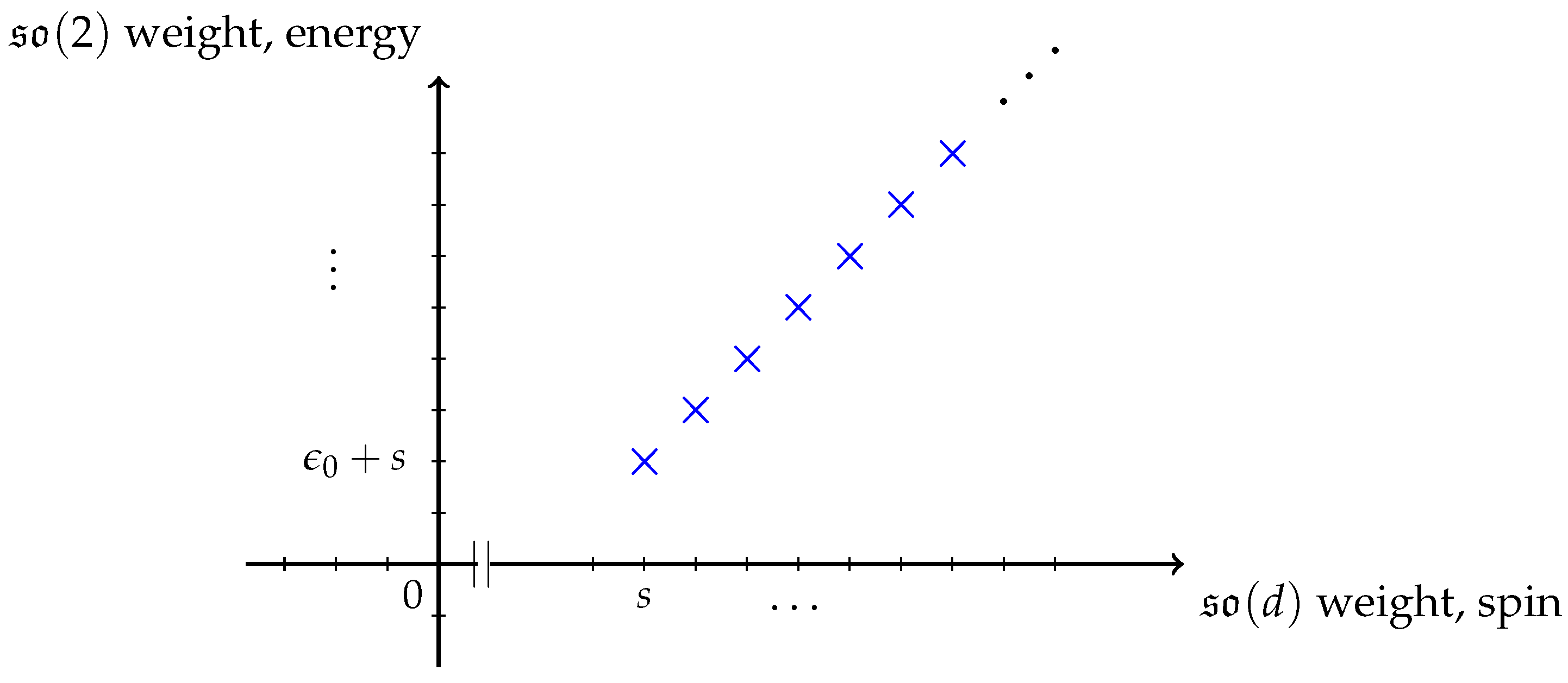
This decomposition can be proven by showing that the character of the module $\mathcal{D}\left(s+r-1;(s^r)\right)$ can be rewritten in the form:

$${\chi }_{[s+r-1;(s^r)]}^{\mathfrak{so}(2,d)}(q,\overrightarrow{x})=\sum _{\sigma =0}^{\infty }{q}^{s+r-1+\sigma }{\chi }_{(s+\sigma ,s^{r-1})}^{\mathfrak{so}(d)}(\overrightarrow{x}),$$

(24)

which is indeed the character of the direct sum of $\mathfrak{so}(2)\oplus \mathfrak{so}(d)$ modules displayed in (22). This was proven in [10], and in practice the idea is simply to use the property of the “universal” function ${\mathcal{P}}^{(d)}(q,\overrightarrow{x})$ that it can be rewritten as:

$${\mathcal{P}}^{(d)}(q,\overrightarrow{x})=\sum _{\sigma ,n=0}^{\infty }{q}^{\sigma +2n}{\chi }_{(\sigma )}^{\mathfrak{so}(d)}(\overrightarrow{x}),$$

(25)

and then perform the tensor product between the $\mathfrak{so}(d)$ characters appearing in the character ${\chi }_{[s+r-1;(s^r)]}^{\mathfrak{so}(2,d)}(q,\overrightarrow{x})$ with ${\chi }_{(s)}^{\mathfrak{so}(d)}(\overrightarrow{x})$. Let us to do that explicitely for $d=4$, where we can take advantage of the exceptional isomorphism $\mathfrak{so}(4)\cong \mathfrak{so}(3)\oplus \mathfrak{so}(3)$ to deal with $\mathfrak{so}(4)$ tensor products:

$$\begin{array}{ccc}\hfill {\chi }_{[s+1;(s,s)]}^{\mathfrak{so}(2,4)}(q,\overrightarrow{x})& =& q^{s+1}\left({\chi }_{(s,s)}^{\mathfrak{so}(4)}(\overrightarrow{x})-q{\chi }_{(s,s-1)}^{\mathfrak{so}(4)}(\overrightarrow{x})+q^2{\chi }_{(s-1,s-1)}^{\mathfrak{so}(4)}(\overrightarrow{x})\right){\mathcal{P}}^{(4)}(q,\overrightarrow{x})\hfill \end{array}$$

(26)

$$\begin{array}{cc}=& {\displaystyle \sum _{n=0}^{\infty }}{q}^{s+1+2n}({\displaystyle \sum _{\sigma =0}^{2s}}{q}^{\sigma }{\displaystyle \sum _{k=0}^{\sigma }}{\chi }_{(s+k,s+k-\sigma )}^{\mathfrak{so}(4)}(\overrightarrow{x})+{\displaystyle \sum _{\sigma =2s+1}^{\infty }}{q}^{\sigma }{\displaystyle \sum _{k=0}^{2s}}{\chi }_{(\sigma +k-s,k-s)}^{\mathfrak{so}(4)}(\overrightarrow{x})\hfill \end{array}$$

(27)

$$\begin{array}{c}-{\displaystyle \sum _{\sigma =0}^{2s-1}}{q}^{\sigma +1}{\displaystyle \sum _{k=0}^{\sigma }}{\chi }_{(s+k,s+k-\sigma -1)}^{\mathfrak{so}(4)}(\overrightarrow{x})-{\displaystyle \sum _{\sigma =1}^{2s-1}}{q}^{\sigma +1}{\displaystyle \sum _{k=0}^{\sigma }}{\chi }_{(s+k-1,s+k-\sigma )}^{\mathfrak{so}(4)}(\overrightarrow{x})\hfill \end{array}$$

(28)

$$\begin{array}{c}-{\displaystyle \sum _{\sigma =2s}^{\infty }}{q}^{\sigma +1}{\displaystyle \sum _{k=0}^{2s-1}}\left[{\chi }_{(\sigma +k+1-s,k-s)}^{\mathfrak{so}(4)}(\overrightarrow{x})+{\chi }_{(\sigma +k-s,k+1-s)}^{\mathfrak{so}(4)}(\overrightarrow{x})\right]\hfill \end{array}$$

(29)

$$\begin{array}{c}+{\displaystyle \sum _{\sigma =0}^{2s-2}}{q}^{\sigma +2}{\displaystyle \sum _{k=0}^{\sigma }}{\chi }_{(s+k-1,s+k-\sigma -1)}^{\mathfrak{so}(4)}(\overrightarrow{x})+{\displaystyle \sum _{\sigma =2s-1}^{\infty }}{q}^{\sigma +2}{\displaystyle \sum _{k=0}^{2s-2}}{\chi }_{(\sigma +k+1-s,k+1-s)}^{\mathfrak{so}(4)}(\overrightarrow{x}))\hfill \end{array}$$

$$\begin{array}{cc}=& {\displaystyle \sum _{n=0}^{\infty }}{q}^{s+1+2n}\left({\displaystyle \sum _{\sigma =0}^{\infty }}{q}^{\sigma }{\chi }_{(s+\sigma ,s)}^{\mathfrak{so}(4)}(\overrightarrow{x})-{\displaystyle \sum _{\sigma =1}^{\infty }}{q}^{\sigma +1}{\chi }_{(s+\sigma -1,s)}^{\mathfrak{so}(4)}(\overrightarrow{x})\right)\hfill \end{array}$$

(30)

$$\begin{array}{cc}=& {\displaystyle \sum _{\sigma =0}^{\infty }}{q}^{s+1+\sigma }{\chi }_{(s+\sigma ,s)}^{\mathfrak{so}(4)}(\overrightarrow{x}).\hfill \end{array}$$

(31)

This decomposition can be illustrated by drawing a “weight diagram”, representing the $\mathfrak{so}(2)$ weight of $\mathfrak{so}(2)\oplus \mathfrak{so}(d)$ modules as a function of the first component of their $\mathfrak{so}(d)$ weights, see Figure 1 below.

The fact the weight diagram of singletons is made out of a single line, noticed in the case of the Dirac singletons of $\mathfrak{so}(2,3)$ in [109] and later extended to singletons in arbitrary dimensions 9 in [5], is the reason for the name “singletons” [102].

(ii)

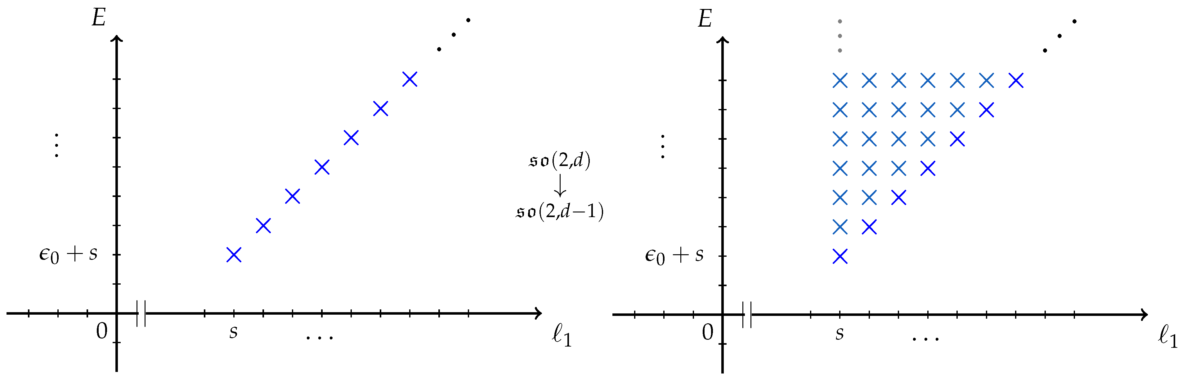
In order to prove the branching rule from $\mathfrak{so}(2,d)$ to $\mathfrak{so}(2,d-1)$, we will compare the $\mathfrak{so}(2)\oplus \mathfrak{so}(d-1)$ decomposition of the $\mathfrak{so}(2,d)$ spin-s singleton on the one hand, obtained by branching 10 the $\mathfrak{so}(d)$ components of the $\mathfrak{so}(2)\oplus \mathfrak{so}(d)$ of these modules displayed in the previous item onto $\mathfrak{so}(d-1)$, to the $\mathfrak{so}(2)\oplus \mathfrak{so}(d-1)$ decomposition of the $\mathfrak{so}(2,d-1)$ module $\mathcal{D}\left(s+r-1;(s^{r-1})\right)$ describing a massless field with spin $(s^{r-1})$. For the sake of brevity, we will only detail the low dimensional case of $\mathfrak{so}(2,4)$ spin-s singletons which captures the idea of the proof, and leave the treatment of the arbitrary dimension case to Appendix B.1.

Let us start by deriving the $\mathfrak{so}(2)\oplus \mathfrak{so}(3)$ decomposition of the $\mathfrak{so}(2,4)$ spin-s singleton module $\mathcal{D}\left(s+1;(s,s)\right)$:

$$\begin{array}{ccc}\hfill \mathcal{D}\left(s+1;(s,s)\right)& \cong & {\displaystyle \underset{\sigma =0}{\overset{\infty }{⨁}}}{\mathcal{D}}_{\mathfrak{so}(2)\oplus \mathfrak{so}(4)}\left(s+1+\sigma ;(s+\sigma ,s)\right)\hfill \end{array}$$

(32)

$$\begin{array}{cc}\stackrel{\mathfrak{so}(2,4)}{\underset{\mathfrak{so}(2,3)}{\downarrow }}& {\displaystyle \underset{\sigma =0}{\overset{\infty }{⨁}}}{\displaystyle \underset{k=0}{\overset{\sigma }{⨁}}}{\mathcal{D}}_{\mathfrak{so}(2)\oplus \mathfrak{so}(3)}\left(s+1+\sigma ;(s+k)\right)\hfill \end{array}$$

(33)

$$\begin{array}{cc}\cong & {\displaystyle \underset{\sigma ,n=0}{\overset{\infty }{⨁}}}{\mathcal{D}}_{\mathfrak{so}(2)\oplus \mathfrak{so}(3)}\left(s+1+\sigma +n;(s+\sigma )\right)\hfill \end{array}$$

(34)

Next, we need to derive the $\mathfrak{so}(2)\oplus \mathfrak{so}(3)$ of a massless spin-s field corresponding to the $\mathfrak{so}(2,3)$ module $\mathcal{D}\left(s+1;(s)\right)$. To do so, we will rewrite its character in a way that makes this decomposition explicit:

$$\begin{array}{ccc}\hfill {\chi }_{[s+1;(s)]}^{\mathfrak{so}(2,3)}(q,x)& =& q^{s+1}\left({\chi }_{(s)}^{\mathfrak{so}(3)}(x)-q{\chi }_{(s-1)}^{\mathfrak{so}(3)}(x)\right){\mathcal{P}}^{(d)}(q,x)\hfill \end{array}$$

(35)

$$\begin{array}{cc}=& {\displaystyle \sum _{\sigma ,n=0}^{\infty }}{q}^{s+1+\sigma +2n}\left({\displaystyle \sum _{\tau =|s-\sigma |}^{s+\sigma }}{\chi }_{(\tau )}^{\mathfrak{so}(3)}(x)-q{\displaystyle \sum _{\tau =|s-1-\sigma |}^{s-1+\sigma }}{\chi }_{(\tau )}^{\mathfrak{so}(3)}(x)\right)\hfill \end{array}$$

(36)

$$\begin{array}{cc}=& {\displaystyle \sum _{n=0}^{\infty }}{q}^{s+1+2n}\left({\chi }_{(s)}^{\mathfrak{so}(3)}+{\displaystyle \sum _{\sigma =1}^{\infty }}{q}^{\sigma }\left[{\displaystyle \sum _{\tau =|s-\sigma |}^{s+\sigma }}{\chi }_{(\tau )}^{\mathfrak{so}(3)}(x)-{\displaystyle \sum _{\tau =|s-\sigma |}^{s+\sigma -2}}{\chi }_{(\tau )}^{\mathfrak{so}(3)}(x)\right]\right)\hfill \end{array}$$

(37)

$$\begin{array}{cc}=& {\displaystyle \sum _{n=0}^{\infty }}{q}^{s+1+2n}(1+q){\displaystyle \sum _{\sigma =0}^{\infty }}{q}^{\sigma }{\chi }_{(s+\sigma )}^{\mathfrak{so}(3)}(x)={\displaystyle \sum _{\sigma ,n=0}^{\infty }}{q}^{s+1+\sigma +n}{\chi }_{(s+\sigma )}^{\mathfrak{so}(3)}(x),\hfill \end{array}$$

(38)

where we used the property (25) of the function ${\mathcal{P}}^{(4)}(q,\overrightarrow{x})$, namely

$${\mathcal{P}}^{(4)}(q,\overrightarrow{x})=\sum _{s,n=0}^{\infty }{q}^{s+2n}{\chi }_{(s)}^{\mathfrak{so}(4)}(\overrightarrow{x}).$$

(39)

This proves that the decomposition of the $\mathfrak{so}(2,3)$ module of a massless spin-s field in AdS${}_4$ reads:

$$\mathcal{D}\left(s+1;(s)\right)\cong \underset{\sigma ,n=0}{\overset{\infty }{⨁}}{\mathcal{D}}_{\mathfrak{so}(2)\oplus \mathfrak{so}(3)}\left(s+1+\sigma +n;(s+\sigma )\right),$$

(40)

which coincide with the $\mathfrak{so}(2)\oplus \mathfrak{so}(3)$ decomposition obtained after branching the $\mathfrak{so}(2,4)$ spin-s singleton module onto $\mathfrak{so}(2,3)$, i.e., we indeed have

$$\mathcal{D}\left(s+1;(s,s)\right)\stackrel{\mathfrak{so}(2,4)}{\underset{\mathfrak{so}(2,3)}{\downarrow }}\mathcal{D}\left(s+1;(s)\right).$$

(41)

This can be graphically seen by implementing the branching rule of the weight diagram in Figure 2. Indeed, the branching rule for the $\mathfrak{so}(2r)$ irrep $(s+\sigma ,s^{r-1})$ is:

$$(s+\sigma ,s^{r-1})\stackrel{\mathfrak{so}(2,d)}{\underset{\mathfrak{so}(2,d-1)}{\downarrow }}\underset{k=0}{\overset{\sigma }{⨁}}(s+k,s^{r-2}),$$

(42)

which means that one should add on each line of the weight diagram (representing the $\mathfrak{so}(d)$ modules appearing at fixed energy, or $\mathfrak{so}(2)$ weight) in Figure 2 a dot at each value of ${\ell }_1$ to the left of the orignal one until ${\ell }_1=s$ is reached. By doing so, an infinite wedge whose tip has coordinates $(E=s+{ϵ}_0,{\ell }_1=s)$ precisely corresponding to the weight diagram of a massless field of spin given by a rectangular Young diagram on maximal height and length s as can be seen from (40) for $d=3$ and in Appendix B.1 for arbitrary odd values of d.

 ☐

We did not, in the previous review of the proofs of the listed properties in Theorem 1, cover the branching rule of the $\mathfrak{so}(2,d)$ singletons onto $\mathfrak{iso}(1,d-1)$ or $\mathfrak{so}(1,d)$ for the following reasons:

• From $\mathfrak{so}(2,d)$ to $\mathfrak{iso}(1,d-1)$. As far as the branching rule from $\mathfrak{so}(2,d)$ to $\mathfrak{so}(1,d-1)$ are concerned, it can be recovered, assuming that the following diagram is commutative:

  (43)

  i.e., by combining the branching rule from $\mathfrak{so}(2,d)$ to $\mathfrak{so}(2,d-1)$ and an Inönü-Wigner contraction. That is to say, it is equivalent (i) to branch a representation ${\mathcal{D}}_{\mathfrak{so}(2,d)}$ from $\mathfrak{so}(2,d)$ onto $\mathfrak{so}(2,d-1)$ and then perform a Inönü-Wigner contraction by sending the cosmological constant λ to zero to obtain a representation ${\mathcal{D}}_{\mathfrak{iso}(1,d-1)}$ of $\mathfrak{iso}(1,d-1)$, and (ii) to branch the $\mathfrak{so}(2,d)$ module ${\mathcal{D}}_{\mathfrak{iso}(1,d-1)}$ onto $\mathfrak{iso}(1,d-1)$ to obtain the same module ${\mathcal{D}}_{\mathfrak{iso}(1,d-1)}$ than previously. Under this assumption, we can use the branching rule (23) of the $\mathfrak{so}(2,d)$ singleton module onto $\mathfrak{so}(2,d-1)$ and then contracting it to a $\mathfrak{iso}(1,d-1)$ instead of deriving the branching rule from $\mathfrak{so}(2,d)$ onto $\mathfrak{iso}(1,d-1)$. The Inönü-Wigner contraction for massless fields in AdS${}_{d+1}$ (i.e., $\mathfrak{so}(2,d)$ modules) is known as the Brink-Metsaev-Vasiliev mechanism [112], which was proven in [65,66,72]. This mechanism states that massless $\mathfrak{so}(2,d)$ UIRs of spin given by a $\mathfrak{so}(d)$ Young diagram $\mathbb{Y}$ contracts to the direct sum of massless UIRs of the Poincaré algebra with spin given by all of the Young diagrams obtained from the branching rule of $\mathbb{Y}$ except those where boxes in the first block of $\mathbb{Y}$ have been removed. Higher-spin singleton, as well as the massless $\mathfrak{so}(2,d-1)$ module onto which they branch being labelled by a rectangular Young diagram, the BMV mechanism implies that they contract to a single $\mathfrak{iso}(1,d-1)$ i.e.,

  $${\mathcal{D}}_{\mathfrak{so}(2,d)}\left(s+r-1;(s^r)\right)\stackrel{\mathfrak{so}(2,d)}{\underset{\mathfrak{so}(2,d-1)}{\downarrow }}{\mathcal{D}}_{\mathfrak{so}(2,d-1)}\left(s+r-1;(s^{r-1})\right)\underset{\lambda \to 0}{⟶}{\mathcal{D}}_{\mathfrak{iso}(1,d-1)}\left(m=0;(s^{r-1})\right),$$

  (44)

  as shown in [5].
• From $\mathfrak{so}(2,d)$ to $\mathfrak{so}(1,d)$. The $\mathfrak{so}(1,d)$ generalised Verma modules are induced by, and decompose into, $\mathfrak{so}(1,1)\oplus \mathfrak{so}(d-1)$ modules instead of $\mathfrak{so}(2)\oplus \mathfrak{so}(d-1)$ in the case of $\mathfrak{so}(2,d-1)$. As a consequence, the method used previously consisting in relying on the common $\mathfrak{so}(2)\oplus \mathfrak{so}(d-1)$ cannot be applied here and we will therefore refer to the original paper [5] for the proof of that branching rule.

3.2. Non-Unitary, Higher-Order Extension

Higher-order extension of the Dirac singletons (i.e., the scalar and spinor ones) are non-unitary $\mathfrak{so}(2,d)$ modules that share the crucial field theoretical property of singletons mentioned above, namely they correspond to AdS (scalar and spinor) field that do not propagate local degree of freedom in the bulk. They have been considered in [6] as well as in [82] where the confinement to the conformal boundary of these remarkable fields was highlighted, but were excluded from the exhaustive work 11 [5] because they fall below the unitary bound for representations of $\mathfrak{so}(2,d)$ (recalled in Subsection 3.1).

Definition 2 (Higher-order Dirac singletons).

The scalar and spinor, order-ℓ Dirac singletons are the $\mathfrak{so}(2,d)$ modules $\mathcal{D}\left({ϵ}_0^{(\ell )};\mathbf{0}\right)$ and $\mathcal{D}\left({ϵ}_{1/2}^{(\ell )};\frac{\mathbf{1}}{\mathbf{2}}\right)$ respectively, where

$${ϵ}_0^{(\ell )}:=\frac{d-2\ell }{2},and{ϵ}_{1/2}^{(\ell )}:=\frac{d+1-2\ell }{2}\equiv {ϵ}_0^{(\ell )}+\frac{1}{2},$$

(45)

and which are defined as the quotient:

$${\mathrm{Rac}}_{\ell }:=\mathcal{D}\left({ϵ}_0^{(\ell )};\mathbf{0}\right)\cong \frac{\mathcal{V}\left({ϵ}_0^{(\ell )};\mathbf{0}\right)}{\mathcal{D}\left(d-{ϵ}_0^{(\ell )};\mathbf{0}\right)},and{\mathrm{Di}}_{\ell }:=\mathcal{D}\left({ϵ}_{1/2}^{(\ell )};\frac{\mathbf{1}}{\mathbf{2}}\right)\cong \frac{\mathcal{V}\left({ϵ}_{1/2}^{(\ell )};\frac{\mathbf{1}}{\mathbf{2}}\right)}{\mathcal{D}\left(d-{ϵ}_{1/2}^{(\ell )};\frac{\mathbf{1}}{\mathbf{2}}\right)}.$$

(46)

Their character read:

$${\chi }_{{\mathrm{Rac}}_{\ell }}^{\mathfrak{so}(2,d)}(q,\overrightarrow{x})=q^{{ϵ}_0^{(\ell )}}(1-q^{2\ell }){\mathcal{P}}^{(d)}(q,\overrightarrow{x}),and{\chi }_{{\mathrm{Di}}_{\ell }}^{\mathfrak{so}(2,d)}(q,\overrightarrow{x})=q^{{ϵ}_{1/2}^{(\ell )}}(1-q^{2\ell -1}){\chi }_{\frac{\mathbf{1}}{\mathbf{2}}}^{\mathfrak{so}(d)}(\overrightarrow{x}){\mathcal{P}}^{(d)}(q,\overrightarrow{x}).$$

(47)

These modules are non-unitary for $\ell >1$, whereas they correspond to the original (unitary) Dirac singletons of Definition 1 for $\ell =1$.

On top of the confinement property, the ${\mathrm{Rac}}_{\ell }$ and ${\mathrm{Di}}_{\ell }$ singletons also possess properties analogous to those of their unitary counterparts reviewed in Theorem 1. Specifically, they can be decomposed as several direct sum of $\mathfrak{so}(2)\oplus \mathfrak{so}(d)$ modules, making up not only one but now several lines in the weight diagram, and they obey a branching rule (from $\mathfrak{so}(2,d)$ to $\mathfrak{so}(2,d-1)$) similar to that of $\mathrm{Rac}$ and $\mathrm{Di}$. The properties of the higher-order Dirac singletons are summed up below.

Proposition 1 (Properties of Rac_ℓ and Di_ℓ).

The $\mathfrak{so}(2)\oplus \mathfrak{so}(d)$ decomposition of the order-ℓ scalar and spinor singletons respectively read 12:

$$\mathcal{D}\left({ϵ}_0^{(\ell )};\mathbf{0}\right)\cong \underset{k=0}{\overset{\ell -1}{⨁}}\underset{\sigma =0}{\overset{\infty }{⨁}}{\mathcal{D}}_{\mathfrak{so}(2)\oplus \mathfrak{so}(d)}\left({ϵ}_0^{(\ell )}+\sigma +2k;(\sigma )\right),$$

(48)

and

$$\mathcal{D}\left({ϵ}_{1/2}^{(\ell )};\frac{\mathbf{1}}{\mathbf{2}}\right)\cong \underset{k=0}{\overset{2(\ell -1)}{⨁}}\underset{\sigma =0}{\overset{\infty }{⨁}}{\mathcal{D}}_{\mathfrak{so}(2)\oplus \mathfrak{so}(d)}\left({ϵ}_{1/2}^{(\ell )}+\sigma +k;(\sigma +\frac{1}{2},{(\frac{1}{2})}^{r-1})\right).$$

(49)

These two modules obey the following branching rules 13:

$$\mathcal{D}\left({ϵ}_0^{(\ell )};\mathbf{0}\right)\stackrel{\mathfrak{so}(2,d)}{\underset{\mathfrak{so}(2,d-1)}{\downarrow }}\underset{k=0}{\overset{2\ell -1}{⨁}}\mathcal{D}\left({ϵ}_0^{(\ell )}+k;\mathbf{0}\right),$$

(50)

and

$$\mathcal{D}\left({ϵ}_{1/2}^{(\ell )};\frac{\mathbf{1}}{\mathbf{2}}\right)\stackrel{\mathfrak{so}(2,d)}{\underset{\mathfrak{so}(2,d-1)}{\downarrow }}\underset{k=0}{\overset{2(\ell -1)}{⨁}}\mathcal{D}\left({ϵ}_{1/2}^{(\ell )}+k;\frac{\mathbf{1}}{\mathbf{2}}\right).$$

(51)

Proof. 

As previsouly, we will use the property (25) of the function ${\mathcal{P}}^{(d)}(q,\overrightarrow{x})$ to rewrite the characters of the order-ℓ scalar and spinor singletons (47) as a sum of $\mathfrak{so}(2)\oplus \mathfrak{so}(d)$ characters, starting with the scalar ${\mathrm{Rac}}_{\ell }$:

$$\begin{array}{ccc}\hfill {\chi }_{{\mathrm{Rac}}_{\ell }}^{\mathfrak{so}(2,d)}(q,\overrightarrow{x})& =& q^{{ϵ}_0^{(\ell )}}(1-q^{2\ell }){\mathcal{P}}^{(d)}(q,\overrightarrow{x})={\displaystyle \sum _{\sigma ,n=0}^{\infty }}{q}^{{ϵ}_0^{(\ell )}+\sigma +2n}(1-q^{2\ell }){\chi }_{(\sigma )}^{\mathfrak{so}(d)}(\overrightarrow{x})\hfill \end{array}$$

(52)

$$\begin{array}{cc}=& {\displaystyle \sum _{k=0}^{\ell -1}}{\displaystyle \sum _{\sigma =0}^{\infty }}{q}^{{ϵ}_0^{(\ell )}+2k+\sigma }{\chi }_{(\sigma )}^{\mathfrak{so}(d)}(\overrightarrow{x})\hfill \end{array}$$

(53)

$$\begin{array}{ccc}\hfill \iff {\mathrm{Rac}}_{\ell }& =& {\displaystyle \underset{k=0}{\overset{\ell -1}{⨁}}}{\displaystyle \underset{\sigma =0}{\overset{\infty }{⨁}}}{\mathcal{D}}_{\mathfrak{so}(2)\oplus \mathfrak{so}(d)}\left({ϵ}_0^{(\ell )}+2k+\sigma ;(\sigma )\right).\hfill \end{array}$$

(54)

For the ${\mathrm{Di}}_{\ell }$ singleton we will also need the $\mathfrak{so}(d)$ tensor product rule:

$$(\sigma )\otimes \frac{\mathbf{1}}{\mathbf{2}}=(\sigma +\frac{1}{2},{(\frac{1}{2})}^{r-1})\oplus (\sigma -\frac{1}{2},{(\frac{1}{2})}^{r-1}),\mathrm{for}\sigma ⩾1.$$

(55)

Using the above identity and proceeding similarly to the scalar case, we end up with:

$$\begin{array}{ccc}\hfill {\chi }_{{\mathrm{Di}}_{\ell }}^{\mathfrak{so}(2,d)}(q,\overrightarrow{x})& =& q^{{ϵ}_{1/2}^{(\ell )}}(1-q^{2\ell -1}){\chi }_{\frac{\mathbf{1}}{\mathbf{2}}}^{\mathfrak{so}(d)}(\overrightarrow{x}){\mathcal{P}}^{(d)}(q,\overrightarrow{x})\hfill \end{array}$$

(56)

$$\begin{array}{cc}=& {\displaystyle \sum _{n=0}^{\infty }}{q}^{{ϵ}_{1/2}^{(\ell )}+2n}(1-q^{2\ell -1})\left({\displaystyle \sum _{\sigma =0}^{\infty }}{q}^{\sigma }{\chi }_{(\sigma +\frac{1}{2},{(\frac{1}{2})}^{r-1})}^{\mathfrak{so}(d)}(\overrightarrow{x})+{\displaystyle \sum _{\sigma =1}^{\infty }}{q}^{\sigma }{\chi }_{(\sigma -\frac{1}{2},{(\frac{1}{2})}^{r-1})}^{\mathfrak{so}(d)}(\overrightarrow{x})\right)\hfill \end{array}$$

(57)

$$\begin{array}{cc}=& {\displaystyle \sum _{n,\sigma =0}^{\infty }}{q}^{{ϵ}_{1/2}^{(\ell )}+2n+\sigma }(1-q^{2\ell -1})(1+q){\chi }_{(\sigma +\frac{1}{2},{(\frac{1}{2})}^{r-1})}^{\mathfrak{so}(d)}(\overrightarrow{x})\hfill \end{array}$$

(58)

$$\begin{array}{cc}=& {\displaystyle \sum _{k=0}^{2(\ell -1)}}{\displaystyle \sum _{\sigma =0}^{\infty }}{q}^{{ϵ}_{1/2}^{(\ell )}+k+\sigma }{\chi }_{(\sigma +\frac{1}{2},{(\frac{1}{2})}^{r-1})}^{\mathfrak{so}(d)}(\overrightarrow{x})\hfill \end{array}$$

(59)

$$\begin{array}{ccc}\hfill \iff {\mathrm{Di}}_{\ell }& =& {\displaystyle \underset{k=0}{\overset{2(\ell -1)}{⨁}}}{\displaystyle \underset{\sigma =0}{\overset{\infty }{⨁}}}{\mathcal{D}}_{\mathfrak{so}(2)\oplus \mathfrak{so}(d)}\left({ϵ}_{1/2}^{(\ell )}+\sigma +k;(\sigma +\frac{1}{2},{(\frac{1}{2})}^{r-1})\right).\hfill \end{array}$$

(60)

To prove the branching rule (50) and (51), we will follow the same strategy as previously, namely we will compare the $\mathfrak{so}(2)\oplus \mathfrak{so}(d-1)$ decomposition of the two sides of these identities. This decomposition reads, for the ${\mathrm{Rac}}_{\ell }$ singleton:

$$\begin{array}{ccc}\hfill \mathcal{D}\left({ϵ}_0^{(\ell )};\mathbf{0}\right)& \cong & {\displaystyle \underset{k=0}{\overset{\ell -1}{⨁}}}{\displaystyle \underset{\sigma =0}{\overset{\infty }{⨁}}}{\mathcal{D}}_{\mathfrak{so}(2)\oplus \mathfrak{so}(d)}\left({ϵ}_0^{(\ell )}+\sigma +2k;(\sigma )\right)\hfill \end{array}$$

(61)

$$\begin{array}{cc}\stackrel{\mathfrak{so}(2,d)}{\underset{\mathfrak{so}(2,d-1)}{\downarrow }}& {\displaystyle \underset{k=0}{\overset{\ell -1}{⨁}}}{\displaystyle \underset{\sigma =0}{\overset{\infty }{⨁}}}{\displaystyle \underset{n=0}{\overset{\sigma }{⨁}}}{\mathcal{D}}_{\mathfrak{so}(2)\oplus \mathfrak{so}(d-1)}\left({ϵ}_0^{(\ell )}+\sigma +2k;(n)\right)\hfill \end{array}$$

(62)

$$\begin{array}{cc}\cong & {\displaystyle \underset{k=0}{\overset{\ell -1}{⨁}}}{\displaystyle \underset{\sigma =0}{\overset{\infty }{⨁}}}{\displaystyle \underset{n=0}{\overset{\infty }{⨁}}}{\mathcal{D}}_{\mathfrak{so}(2)\oplus \mathfrak{so}(d-1)}\left({ϵ}_0^{(\ell )}+\sigma +2k+n;(\sigma )\right),\hfill \end{array}$$

(63)

whereas for the ${\mathrm{Di}}_{\ell }$ singleton:

$$\begin{array}{ccc}\hfill \mathcal{D}\left({ϵ}_{1/2}^{(\ell )};\frac{\mathbf{1}}{\mathbf{2}}\right)& \cong & {\displaystyle \underset{k=0}{\overset{2(\ell -1)}{⨁}}}{\displaystyle \underset{\sigma =0}{\overset{\infty }{⨁}}}{\mathcal{D}}_{\mathfrak{so}(2)\oplus \mathfrak{so}(d)}\left({ϵ}_{1/2}^{(\ell )}+\sigma +k;(\sigma +\frac{1}{2},{(\frac{1}{2})}^{r-1})\right)\hfill \end{array}$$

(64)

$$\begin{array}{cc}\stackrel{\mathfrak{so}(2,d)}{\underset{\mathfrak{so}(2,d-1)}{\downarrow }}& {\displaystyle \underset{k=0}{\overset{2(\ell -1)}{⨁}}}{\displaystyle \underset{\sigma =0}{\overset{\infty }{⨁}}}{\displaystyle \underset{n=0}{\overset{\sigma }{⨁}}}{\mathcal{D}}_{\mathfrak{so}(2)\oplus \mathfrak{so}(d-1)}\left({ϵ}_{1/2}^{(\ell )}+\sigma +k;(n+\frac{1}{2},{(\frac{1}{2})}^{r-1})\right)\hfill \end{array}$$

(65)

$$\begin{array}{cc}\cong & {\displaystyle \underset{k=0}{\overset{2(\ell -1)}{⨁}}}{\displaystyle \underset{\sigma =0}{\overset{\infty }{⨁}}}{\displaystyle \underset{n=0}{\overset{\infty }{⨁}}}{\mathcal{D}}_{\mathfrak{so}(2)\oplus \mathfrak{so}(d-1)}\left({ϵ}_{1/2}^{(\ell )}+\sigma +k+n;(\sigma +\frac{1}{2},{(\frac{1}{2})}^{r-1})\right).\hfill \end{array}$$

(66)

On the other hand, the character of an irreducible $\mathfrak{so}(2,d-1)$ module $\mathcal{D}\left(\Delta ;\mathbf{0}\right)\equiv \mathcal{V}\left(\Delta ;\mathbf{0}\right)$, i.e., a generalised Verma module which does not contain a submodule 14 can be rewritten as:

$$\begin{array}{ccc}\hfill {\chi }_{[\Delta ;\mathbf{0}]}^{\mathfrak{so}(2,d-1)}(q,\overrightarrow{x})& =& q^{\Delta }{\mathcal{P}}^{(d-1)}(q,\overrightarrow{x})={\displaystyle \sum _{\sigma ,n=0}^{\infty }}{q}^{\Delta +2n+\sigma }{\chi }_{(\sigma )}^{\mathfrak{so}(d-1)}(\overrightarrow{x})\hfill \end{array}$$

(67)

$$\begin{array}{ccc}\hfill \iff \mathcal{D}\left(\Delta ;\mathbf{0}\right)& \cong & {\displaystyle \underset{\sigma =0}{\overset{\infty }{⨁}}}{\displaystyle \underset{n=0}{\overset{\infty }{⨁}}}{\mathcal{D}}_{\mathfrak{so}(2)\oplus \mathfrak{so}(d-1)}\left(\Delta +\sigma +2n;(\sigma )\right)\hfill \end{array}$$

(68)

As a consequence,

$$\mathcal{D}\left({ϵ}_0^{(\ell )}+2k;\mathbf{0}\right)\oplus \mathcal{D}\left({ϵ}_0^{(\ell )}+2k+1;\mathbf{0}\right)\cong {\displaystyle \underset{\sigma =0}{\overset{\infty }{⨁}}}{\displaystyle \underset{n=0}{\overset{\infty }{⨁}}}{\mathcal{D}}_{\mathfrak{so}(2)\oplus \mathfrak{so}(d-1)}\left({ϵ}_0^{(\ell )}+\sigma +n+2k;(\sigma )\right),$$

(69)

which proves (50). Finally, an irreducible $\mathfrak{so}(2,d-1)$ module $\mathcal{D}\left(\Delta ;\frac{\mathbf{1}}{\mathbf{2}}\right)\equiv \mathcal{V}\left(\Delta ;\frac{\mathbf{1}}{\mathbf{2}}\right)$ admits the following $\mathfrak{so}(2)\oplus \mathfrak{so}(d-1)$ decomposition:

$$\begin{array}{ccc}\hfill {\chi }_{[\Delta ;\frac{\mathbf{1}}{\mathbf{2}}]}^{\mathfrak{so}(2,d-1)}(q,\overrightarrow{x})& =& q^{\Delta }{\chi }_{\frac{\mathbf{1}}{\mathbf{2}}}^{\mathfrak{so}(d-1)}(\overrightarrow{x}){\mathcal{P}}^{(d-1)}(q,\overrightarrow{x})\hfill \end{array}$$

(70)

$$\begin{array}{cc}=& {\displaystyle \sum _{n=0}^{\infty }}{q}^{\Delta +2n}\left({\displaystyle \sum _{\sigma =0}^{\infty }}{q}^{\sigma }{\chi }_{(\sigma +\frac{1}{2},{(\frac{1}{2})}^{r-1})}^{\mathfrak{so}(d-1)}(\overrightarrow{x})+{\displaystyle \sum _{\sigma =1}^{\infty }}{q}^{\sigma }{\chi }_{(\sigma -\frac{1}{2},{(\frac{1}{2})}^{r-1})}^{\mathfrak{so}(d-1)}(\overrightarrow{x})\right)\hfill \end{array}$$

(71)

$$\begin{array}{cc}=& {\displaystyle \sum _{\sigma =0}^{\infty }}{\displaystyle \sum _{n=0}^{\infty }}{q}^{\Delta +\sigma +n}{\chi }_{(\sigma +\frac{1}{2},{(\frac{1}{2})}^{r-1})}^{\mathfrak{so}(d-1)}(\overrightarrow{x})\hfill \end{array}$$

(72)

$$\begin{array}{ccc}\hfill \iff \mathcal{D}\left(\Delta ;\frac{\mathbf{1}}{\mathbf{2}}\right)& \cong & {\displaystyle \underset{\sigma =0}{\overset{\infty }{⨁}}}{\displaystyle \underset{n=0}{\overset{\infty }{⨁}}}{\mathcal{D}}_{\mathfrak{so}(2)\oplus \mathfrak{so}(d-1)}\left(\Delta +\sigma +n;(\sigma +\frac{1}{2},{(\frac{1}{2})}^{r-1})\right),\hfill \end{array}$$

(73)

thereby proving (51). ☐

The branching rule (50) and (51) reproduce that given in [5,8] (and rederived in [113]) for the Rac and Di singletons upon setting $\ell =1$, and extend them to the higher-order Dirac singletons ${\mathrm{Rac}}_{\ell }$ and ${\mathrm{Di}}_{\ell }$.

From a CFT point of view, the order-ℓ scalar and spinor singletons correspond to respectively a non-unitary fundamental scalar or spinor fields of respective conformal weight ${ϵ}_0^{(\ell )}$ and ${ϵ}_{1/2}^{(\ell )}$, and respectively subject to an order $2\ell$ and $2\ell -1$ wave equation (see e.g., [82] for more details). The spectrum of current of these CFT contains an infinite tower of partially conserved totally symmetric currents of arbitrary spin, which should be dual to partially massless gauge fields in the bulk [114].

3.3. Candidates for Higher-Spin Higher-Order Singletons

The extension we will be concerned with corresponds to the $\mathfrak{so}(2,d)$ module, for $d=2r$:

$$\mathcal{D}\left(s+\frac{d}{2}-t;(s^r)\right)\cong \frac{\mathcal{V}\left(s+\frac{d}{2}-t;(s^r)\right)}{\mathcal{D}\left(s+\frac{d}{2};(s^{r-1},s-t)\right)},\mathrm{for}1⩽t⩽s,$$

(74)

whose structure is similar to the unitary spin-s singletons for $s⩾1$ in the sense that the various submodule to be modded out of $\mathcal{V}(s+\frac{d}{2}-t;(s^r))$ are defined throught the sequence:

$$\mathcal{D}\left(s+\frac{d}{2}+k;(s^{r-k-1},{(s-1)}^k,s-t)\right):=\frac{\mathcal{V}\left(s+\frac{d}{2}+k;(s^{r-k-1},{(s-1)}^k,s-t)\right)}{\mathcal{D}\left(s+\frac{d}{2}+k+1;(s^{r-k-2},{(s-1)}^{k+1},s-t)\right)},$$

(75)

for $0⩽k⩽r-2$ and $\mathcal{D}\left(s+d-1;({(s-1)}^{r-1},s-t)\right)\equiv \mathcal{V}\left(s+d-1;({(s-1)}^{r-1},s-t)\right)$. In other words, except for the first submodule which is obtained by increasing the $\mathfrak{so}(2)$ weight of t units and removing t boxes from the last row of the rectangular Young diagram $(s^r)$ labelling the irreducible module, the sequence of nested submodules are related to one another by adding one unit to the $\mathfrak{so}(2)$ weight of the previous submodule and removing one box in the row above the previously amputated row. Correspondingly, the character of this module reads:

$${\chi }_{[s+\frac{d}{2}-t;(s^r)]}^{\mathfrak{so}(2,d)}(q,\overrightarrow{x})=q^{s+\frac{d}{2}-t}\left({\chi }_{(s^r)}^{\mathfrak{so}(d)}(\overrightarrow{x})+\sum _{k=0}^{r-1}{(-)}^{k+1}{q}^{t+k}{\chi }_{(s^{r-1-k},{(s-1)}^k,s-t)}^{\mathfrak{so}(d)}(\overrightarrow{x})\right){\mathcal{P}}^{(d)}(q,\overrightarrow{x}).$$

(76)

This definition encompasses the unitary spin-s singletons, which correspond to the case $t=1$ saturating the unitarity bound. For $t>1$ (but always $t⩽s$), the module (74) is non-unitary and describes a depth-t partially-massless field of spin $(s^r)$. The spin being given by a rectangular Young diagram, we will refer to this class of module as “rectangular” partially massless (RPM) fields of spin s and depth t. From the boundary point of view, the modules (74) correspond to the curvature a conformal field of spin $(s^{r-1})$ (hence the curvature is given by a tensor of symmetry described by a rectangular Young diagram of length s and height r) obeying a partial conservation law of order t, i.e., taking t symmetrised divergences of this curvature identically vanishes on-shell (see e.g., [115] where the $d=4$ and $t=1$ case was discussed, and [116] for a more details on mixed symmetry conformal field in arbitrary dimensions).

Remark 2.

Notice that formally, the modules of the ${\mathrm{Rac}}_{\ell }$ and ${\mathrm{Di}}_{\ell }$ singletons, as well as the module (74) that we propose here as a higher-spin generalisation of the higher-order scalar and spinor singletons, can be denoted as:

$$\mathcal{D}\left(s+{ϵ}_0^{(t)};(s^r)\right),withs=0,\frac{1}{2},ands\in \mathbb{N}ifd=2r$$

(77)

with ${ϵ}_0^{(t)}=\frac{d-2t}{2}$ as defined in Definition 2. On top of being notationally convenient, this coincidence is actually the reason why the modules (74) are “natural” generalisations of the unitary higher-spin singletons: by introducing the parameter t in this way, one considers a family of modules whose first representative is the unitary singletons whereas for $t>1$ the modules are non-unitary but their structure is almost the same than in the unitary case.

Let us now study what are the counterpart of the properties displayed in Theorem 1 for unitary singletons and Proposition 1 for the ${\mathrm{Rac}}_{\ell }$ and ${\mathrm{Di}}_{\ell }$ singletons, starting with the $\mathfrak{so}(2)\oplus \mathfrak{so}(d)$ decomposition of (74).

Proposition 2 ($\mathfrak{so}(2)\oplus \mathfrak{so}(d)$ decomposition).

The $\mathfrak{so}(2,d)$ module $\mathcal{D}\left(s+r-t;(s^r)\right)$ for $d=2r$, describing a depth-t and spin-s RPM field, admits the following $\mathfrak{so}(2)\oplus \mathfrak{so}(d)$ decomposition:

$$\mathcal{D}\left(s+r-t;(s^r)\right)\cong \underset{\ell =0}{\overset{t-1}{⨁}}\underset{n=0}{\overset{t-1-\ell }{⨁}}\underset{\sigma =\ell }{\overset{\infty }{⨁}}{\mathcal{D}}_{\mathfrak{so}(2)\oplus \mathfrak{so}(d)}\left(s+r-t+\sigma +2n;(s-\ell +\sigma ,s^{r-2},s-\ell )\right).$$

(78)

Equivalently, this property means that the character (76) can bewritten as:

$${\chi }_{[s+r-t;(s^r)]}^{\mathfrak{so}(2,d)}(q,\overrightarrow{x})=\sum _{\ell =0}^{t-1}\sum _{n=0}^{t-1-\ell }\sum _{\sigma =\ell }^{\infty }{q}^{s+r-t+\sigma +2n}{\chi }_{(s+\sigma -\ell ,s^{r-2},s-\ell )}^{\mathfrak{so}(d)}(\overrightarrow{x}).$$

(79)

Proof. 

As previously, we will only focus on the simpler $d=4$ case and leave the proof of this property in arbitrary dimension to Appendix B.2. We will proceed in the exact same way as we did for unitary higher-spin singleton, that is we will use (25) in the character formula (76), so as to rewrite it in the following way:

$$\begin{array}{ccc}\hfill {\chi }_{[s+2-t;(s,s)]}^{\mathfrak{so}(2,4)}(q,\overrightarrow{x})& =& q^{s+2-t}\left({\chi }_{(s,s)}^{\mathfrak{so}(4)}(\overrightarrow{x})-q^t{\chi }_{(s,s-t)}^{\mathfrak{so}(4)}(\overrightarrow{x})+q^{t+1}{\chi }_{(s-1,s-t)}^{\mathfrak{so}(4)}(\overrightarrow{x})\right){\mathcal{P}}^{(4)}(q,\overrightarrow{x})\hfill \end{array}$$

(80)

$$\begin{array}{cc}=& {\displaystyle \sum _{n=0}^{\infty }}{q}^{s+2-t+2n}({\displaystyle \sum _{\sigma =0}^{2s}}{q}^{\sigma }{\displaystyle \sum _{k=0}^{\sigma }}{\chi }_{(s+k,s+k-\sigma )}^{\mathfrak{so}(4)}(\overrightarrow{x})+{\displaystyle \sum _{\sigma =2s+1}^{\infty }}{q}^{\sigma }{\displaystyle \sum _{k=0}^{2s}}{\chi }_{(\sigma +k-s,k-s)}^{\mathfrak{so}(4)}(\overrightarrow{x})\hfill \end{array}$$

(81)

$$\begin{array}{c}-{\displaystyle \sum _{m=0}^t}\left[{\displaystyle \sum _{\sigma =m}^{2s-t}}{q}^{\sigma +t}{\displaystyle \sum _{k=0}^{\sigma }}{\chi }_{(s+k-m,s+k-\sigma -t+m)}^{\mathfrak{so}(4)}(\overrightarrow{x})+{\displaystyle \sum _{\sigma =2s-t+1}^{\infty }}{q}^{\sigma +t}{\displaystyle \sum _{k=0}^{2s-t}}{\chi }_{(\sigma +k+t-s-m,k+m-s)}^{\mathfrak{so}(4)}(\overrightarrow{x})\right]\hfill \end{array}$$

$$\begin{array}{c}+{\displaystyle \sum _{m=0}^{t-1}}[{\displaystyle \sum _{\sigma =m}^{2s-t-1}}{q}^{\sigma +t+1}{\displaystyle \sum _{k=0}^{\sigma }}{\chi }_{(s+k-m-1,s+k-\sigma -t+m)}^{\mathfrak{so}(4)}(\overrightarrow{x})\end{array}$$

(82)

$$\begin{array}{c}+{\displaystyle \sum _{\sigma =2s-t}^{\infty }}{q}^{\sigma +t+1}{\displaystyle \sum _{k=0}^{2s-t-1}}{\chi }_{(\sigma +k+t-s-m,k+m+1-s)}^{\mathfrak{so}(4)}(\overrightarrow{x})\left]\right)\end{array}$$

$$\begin{array}{cc}=& {\displaystyle \sum _{n=0}^{\infty }}{q}^{s+2-t+2n}({\displaystyle \sum _{\sigma =0}^{t-1}}{q}^{\sigma }{\displaystyle \sum _{k=0}^{\sigma }}{\chi }_{(s+k,s+k-\sigma )}^{\mathfrak{so}(4)}(\overrightarrow{x})+{\displaystyle \sum _{m=0}^{t-1}}{\displaystyle \sum _{\sigma =t}^{\infty }}{q}^{\sigma }{\chi }_{(s+\sigma -m,s-m)}^{\mathfrak{so}(4)}(\overrightarrow{x})\hfill \end{array}$$

(83)

$$\begin{array}{c}-{\displaystyle \sum _{m=1}^t}{\displaystyle \sum _{\sigma =m}^{\infty }}{q}^{\sigma +t}{\chi }_{(s+\sigma -m,s-t+m)}^{\mathfrak{so}(4)}(\overrightarrow{x}))\hfill \end{array}$$

(84)

$$\begin{array}{cc}=& {\displaystyle \sum _{n=0}^{\infty }}{q}^{s+2-t+2n}{\displaystyle \sum _{m=0}^{t-1}}\left({\displaystyle \sum _{\sigma =m}^{\infty }}{q}^{\sigma }{\chi }_{(s+\sigma -m,s-m)}^{\mathfrak{so}(4)}(\overrightarrow{x})-{\displaystyle \sum _{\sigma =t-m}^{\infty }}{q}^{\sigma +t}{\chi }_{(s+\sigma -t+m,s-m)}^{\mathfrak{so}(4)}(\overrightarrow{x})\right)\hfill \end{array}$$

(85)

$$\begin{array}{cc}=& {\displaystyle \sum _{n=0}^{\infty }}{q}^{s+2-t+2n}{\displaystyle \sum _{m=0}^{t-1}}{\displaystyle \sum _{\sigma =m}^{\infty }}{q}^{\sigma }(1-q^{2(t-m)}){\chi }_{(s+\sigma -m,s-m)}^{\mathfrak{so}(4)}(\overrightarrow{x})\hfill \end{array}$$

(86)

$$\begin{array}{cc}=& {\displaystyle \sum _{\ell =0}^{t-1}}{\displaystyle \sum _{n=0}^{t-1-\ell }}{\displaystyle \sum _{\sigma =\ell }^{\infty }}{q}^{\sigma +s+2-t+2n}{\chi }_{(s-\ell +\sigma ,s-\ell )}^{\mathfrak{so}(4)}(\overrightarrow{x}),\hfill \end{array}$$

(87)

where we used

$${\displaystyle \sum _{\sigma =0}^{t-1}}{q}^{\sigma }{\displaystyle \sum _{k=0}^{\sigma }}{\chi }_{(s+k,s+k-\sigma )}^{\mathfrak{so}(4)}(\overrightarrow{x})={\displaystyle \sum _{m=0}^{t-1}}{\displaystyle \sum _{\sigma =m}^{t-1}}{q}^{\sigma }{\chi }_{(s+\sigma -m,s-m)}^{\mathfrak{so}(4)}(\overrightarrow{x}),$$

(88)

between (83) and (85). Expression (87) shows that the depth-t PM module $\mathcal{D}\left(s+2-t;(s,s)\right)$ decomposes as the direct sum of $\mathfrak{so}(2)\oplus \mathfrak{so}(4)$ modules:

$$\mathcal{D}\left(s+2-t;(s,s)\right)\cong \underset{\ell =0}{\overset{t-1}{⨁}}\underset{n=0}{\overset{t-1-\ell }{⨁}}\underset{\sigma =\ell }{\overset{\infty }{⨁}}{\mathcal{D}}_{\mathfrak{so}(2)\oplus \mathfrak{so}(4)}\left(s+2-t+\sigma +2n;(s+\sigma -\ell ,s-\ell )\right).$$

(89)

 ☐

With the previous $\mathfrak{so}(2)\oplus \mathfrak{so}(d)$ decomposition at hand, we can now derive the branching rule of the spin-s depth-t RPM module.

Proposition 3 (Branching rule).

The $\mathfrak{so}(2,d)$ module $\mathcal{D}\left(s+r-t;(s^r)\right)$ for $d=2r$, describing a depth-t and spin-s RPM field, branches onto the direct sum of $\mathfrak{so}(2,d-1)$ modules $\mathcal{D}\left(s+r-\tau ;(s^{r-1})\right)$ with $\tau =1,\dots ,t$ describing partially massless fields in AdS${}_d$ of spin $(s^{r-1})$ and with depth-τ:

$$\mathcal{D}\left(s+r-t;(s^r)\right)\stackrel{\mathfrak{so}(2,d)}{\underset{\mathfrak{so}(2,d-1)}{\downarrow }}\underset{\tau =1}{\overset{t}{⨁}}\mathcal{D}\left(s+r-\tau ;(s^{r-1})\right).$$

(90)

Proof. 

Here again we will only display the proof for the low dimensional case $d=4$ in order to illustrate the general mechanism while being not too technically involved, and we leave the treatment in arbitrary dimensions to the Appendix B.2.

In order to prove the branching rule (90) for $\mathfrak{so}(2,4)$, we will compare the $\mathfrak{so}(2)\oplus \mathfrak{so}(3)$ decomposition of the $\mathfrak{so}(2,4)$ spin-s and depth-t singleton (obtained by first branching it onto $\mathfrak{so}(2,3)$) to the $\mathfrak{so}(2)\oplus \mathfrak{so}(3)$ decomposition of the $\mathfrak{so}(2,3)$ spin-s and depth-τ partially massless fields. Let us start with the latter, i.e., derive the $\mathfrak{so}(2)\oplus \mathfrak{so}(3)$ decomposition of the $\mathfrak{so}(2,3)$ module $\mathcal{D}\left(s+2-\tau ;(s)\right)$ using its character:

$$\begin{array}{ccc}\hfill {\chi }_{[s+2-\tau ;(s)]}^{\mathfrak{so}(2,3)}(q,x)& =& q^{s+2-\tau }\left({\chi }_{(s)}^{\mathfrak{so}(3)}(x)-q^{\tau }{\chi }_{(s-\tau )}^{\mathfrak{so}(3)}(x)\right){\mathcal{P}}^{(3)}(q,x)\hfill \end{array}$$

(91)

$$\begin{array}{cc}=& {\displaystyle \sum _{n,\sigma =0}^{\infty }}{q}^{s+2-\tau +\sigma +2n}\left({\displaystyle \sum _{k=|s-\sigma |}^{s+\sigma }}{\chi }_{(k)}^{\mathfrak{so}(3)}(x)-q^{\tau }{\displaystyle \sum _{k=|s-\sigma -\tau |}^{s+\sigma -\tau }}{\chi }_{(k)}^{\mathfrak{so}(3)}(x)\right)\hfill \end{array}$$

(92)

$$\begin{array}{cc}=& {\displaystyle \sum _{n=0}^{\infty }}{q}^{s+2-\tau +2n}\left({\displaystyle \sum _{\sigma =0}^{\infty }}{q}^{\sigma }{\displaystyle \sum _{k=|s-\sigma |}^{s+\sigma }}{\chi }_{(k)}^{\mathfrak{so}(3)}(x)-{\displaystyle \sum _{\sigma =\tau }^{\infty }}{q}^{\sigma }{\displaystyle \sum _{k=|s-\sigma |}^{s+\sigma -2\tau }}{\chi }_{(k)}^{\mathfrak{so}(3)}(x)\right)\hfill \end{array}$$

(93)

$$\begin{array}{cc}=& {\displaystyle \sum _{n=0}^{\infty }}{q}^{s+2-\tau +2n}\left({\displaystyle \sum _{\sigma =0}^{\tau -1}}{q}^{\sigma }{\displaystyle \sum _{k=|s-\sigma |}^{s+\sigma }}{\chi }_{(k)}^{\mathfrak{so}(3)}(x)+{\displaystyle \sum _{\sigma =\tau }^{\infty }}{q}^{\sigma }{\displaystyle \sum _{k=s+\sigma -2\tau +1}^{s+\sigma }}{\chi }_{(k)}^{\mathfrak{so}(3)}(x)\right)\hfill \end{array}$$

(94)

$$\begin{array}{cc}=& {\displaystyle \sum _{\sigma ,n=0}^{\infty }}{\displaystyle \sum _{k=0}^{\tau -1}}{q}^{s+2-\tau +n+\sigma +k}{\chi }_{(s+\sigma -k)}^{\mathfrak{so}(3)}(x).\hfill \end{array}$$

(95)

Hence, the $\mathfrak{so}(2)\oplus \mathfrak{so}(3)$ decomposition of a $\mathfrak{so}(2,3)$ spin-s and depth-τ partially massless field reads:

$$\mathcal{D}\left(s+2-\tau ;(s)\right)\cong \underset{\sigma =0}{\overset{\infty }{⨁}}\underset{n=0}{\overset{\infty }{⨁}}\underset{k=0}{\overset{\tau -1}{⨁}}{\mathcal{D}}_{\mathfrak{so}(2)\oplus \mathfrak{so}(3)}\left(s+2-\tau +n+\sigma +k;(s+\sigma -k)\right).$$

(96)

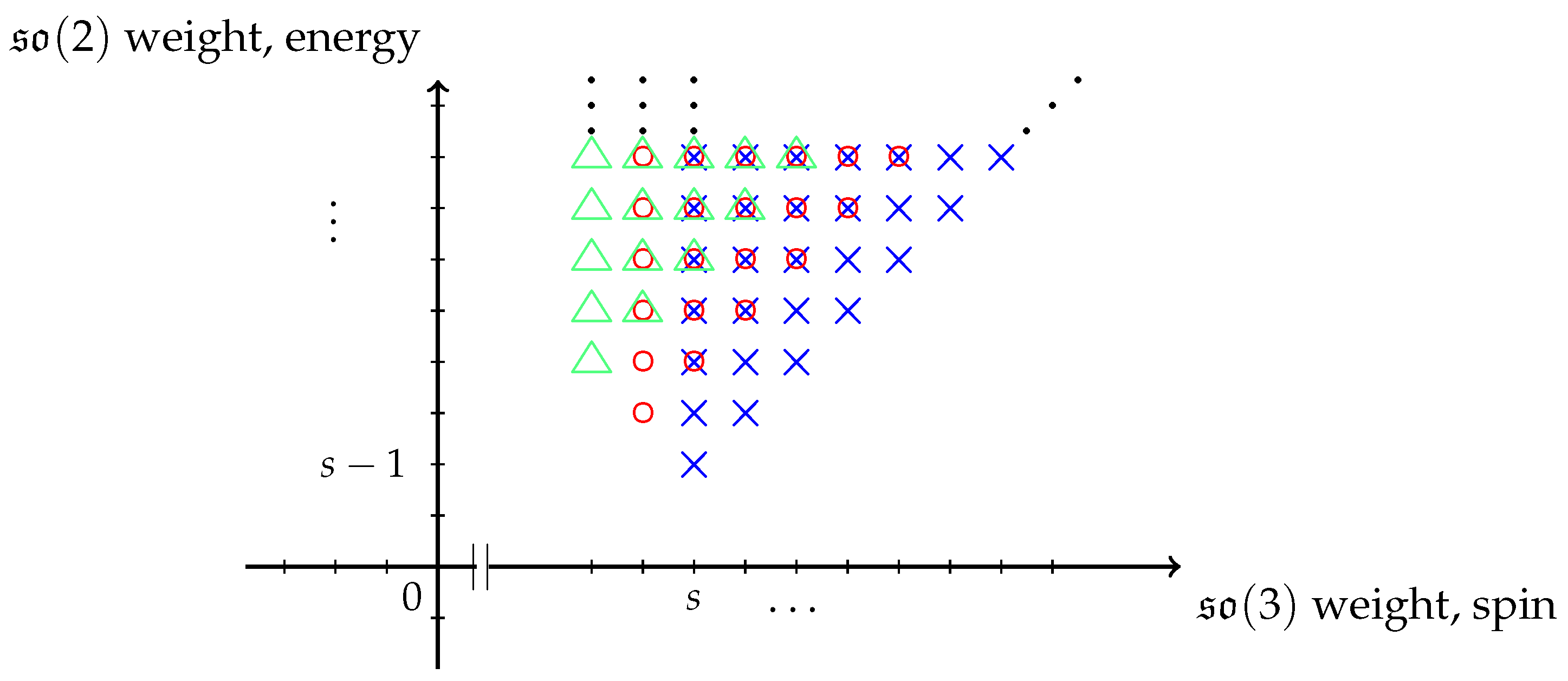
This can be represented graphically by the weight diagram displayed in Figure 3 for $\tau =3$.

Now starting with the $\mathfrak{so}(2)\oplus \mathfrak{so}(4)$ decomposition (78) of the spin-s depth-t PM $\mathfrak{so}(2,4)$ module, we can derive its $\mathfrak{so}(2)\oplus \mathfrak{so}(3)$ decomposition:

$$\begin{array}{ccc}\hfill \mathcal{D}\left(s+2-t;(s,s)\right)& \cong & {\displaystyle \underset{\ell =0}{\overset{t-1}{⨁}}}{\displaystyle \underset{n=0}{\overset{t-1-\ell }{⨁}}}{\displaystyle \underset{\sigma =\ell }{\overset{\infty }{⨁}}}{\mathcal{D}}_{\mathfrak{so}(2)\oplus \mathfrak{so}(4)}\left(s+2-t+\sigma +2n;(s+\sigma -\ell ,s-\ell )\right)\hfill \end{array}$$

(97)

$$\begin{array}{cc}\stackrel{\mathfrak{so}(2,4)}{\underset{\mathfrak{so}(2,3)}{\downarrow }}& {\displaystyle \underset{\ell =0}{\overset{t-1}{⨁}}}{\displaystyle \underset{n=0}{\overset{t-1-\ell }{⨁}}}{\displaystyle \underset{\sigma =\ell }{\overset{\infty }{⨁}}}{\displaystyle \underset{k=0}{\overset{\sigma }{⨁}}}{\mathcal{D}}_{\mathfrak{so}(2)\oplus \mathfrak{so}(3)}\left(s+2-t+\sigma +2n;(s+k-\ell )\right)\hfill \end{array}$$

(98)

$$\begin{array}{cc}\cong & {\displaystyle \underset{\tau =1}{\overset{t}{⨁}}}{\displaystyle \underset{k=0}{\overset{\tau -1}{⨁}}}{\displaystyle \underset{\sigma =0}{\overset{\infty }{⨁}}}{\displaystyle \underset{n=0}{\overset{\infty }{⨁}}}{\mathcal{D}}_{\mathfrak{so}(2)\oplus \mathfrak{so}(3)}\left(s+2-\tau +n+\sigma +k;(s+\sigma -k)\right)\hfill \end{array}$$

(99)

which matches the direct sum of the $\mathfrak{so}(2)\oplus \mathfrak{so}(3)$ decomposition of the spin-s partially massless modules of depth $\tau =1,\dots ,t$, i.e.,

$$\mathcal{D}\left(s+2-t;(s,s)\right)\stackrel{\mathfrak{so}(2,4)}{\underset{\mathfrak{so}(2,3)}{\downarrow }}\underset{\tau =1}{\overset{t}{⨁}}\mathcal{D}\left(s+2-\tau ;(s)\right).$$

(100)

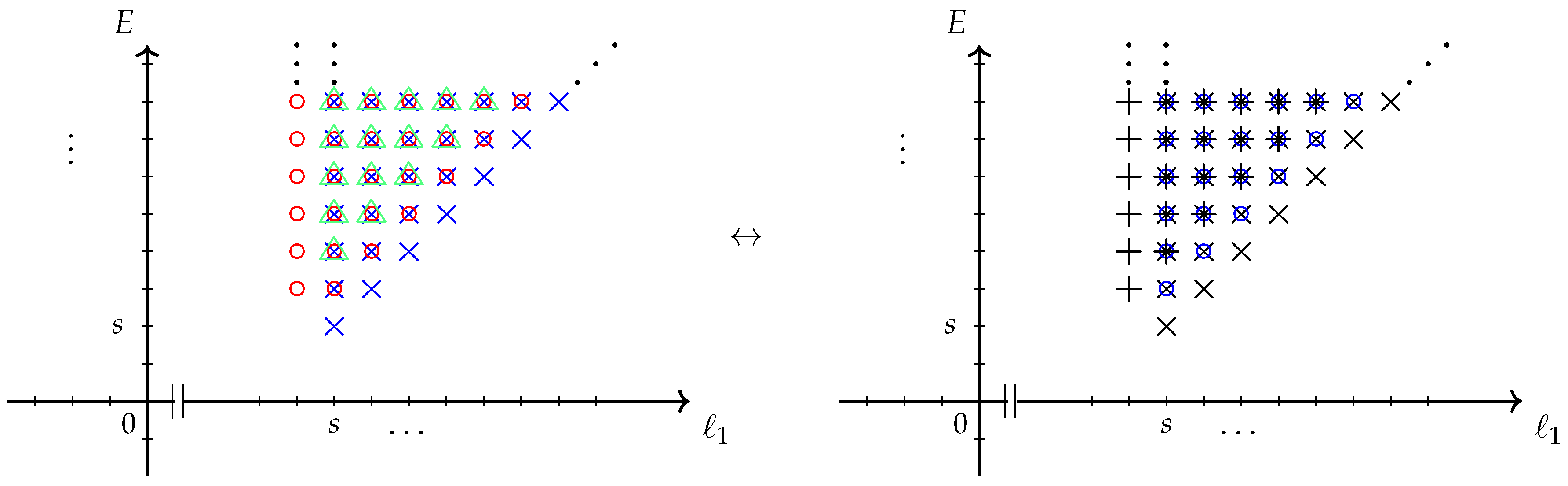
This branching rule can also be represented graphically, by drawing on the one hand the $\mathfrak{so}(2)\oplus \mathfrak{so}(3)$ weight diagram of the spin-s and depth-t RPM field as read from (98) and on the other hand by drawing the $\mathfrak{so}(2)\oplus \mathfrak{so}(3)$ weight diagrams of the partially massless spin-s modules of depth $\tau =1,\dots ,t$, and comparing the two diagrams. This is done for the $t=2$ case in Figure 4 below. ☐

Remark 3.

Notice that the previous Proposition 3 encompasses the case of unitary higher-spin singleton, corresponding to $t=1$. The above decomposition reduce, in this special case $t=1$ to those previously derived and summed up in Theorem 1.

From $\mathfrak{so}(2,d)$ to $\mathfrak{iso}(1,d-1)$.

Again assuming that the diagram (43) is commutative, the branching of the spin-s and depth-t RPM can be obtained by performing an Inönü-Wigner contraction of the $\mathfrak{so}(2,d-1)$ modules. Applying the BMV mechanism to a $\mathfrak{so}(2,d-1)$ partially massless fields of depth-t and spin given by a maximal height rectangular Young diagram yields [65,66,112]:

$${\mathcal{D}}_{\mathfrak{so}(2,d-1)}\left(s+d-r-t;(s^{r-1})\right)\underset{\lambda \to 0}{⟶}\underset{\tau =0}{\overset{t-1}{⨁}}{\mathcal{D}}_{\mathfrak{iso}(1,d-1)}\left(m=0;(s^{r-2},s-\tau )\right).$$

(101)

As a consequence, the branching rule of the $\mathfrak{so}(2,d)$ spin-s and depth-t RPM module onto $\mathfrak{iso}(1,d-1)$ reads:

$${\mathcal{D}}_{\mathfrak{so}(2,d)}\left(s+r-t;(s^r)\right)\stackrel{\mathfrak{so}(2,d)}{\underset{\mathfrak{iso}(1,d-1)}{\downarrow }}\underset{\tau =0}{\overset{t-1}{⨁}}(t-\tau ){\mathcal{D}}_{\mathfrak{iso}(1,d-1)}\left(m=0;(s^{r-2},s-\tau )\right).$$

(102)

At this point, a few comments are in order. As emphasised in the first part of this section, the crucial properties of unitary singletons is that $(i)$ they constitute the class of representations that can be lifted from $\mathfrak{so}(2,d-1)$ to $\mathfrak{so}(2,d)$, i.e., they are AdS fields that are also conformal, and $(ii)$ they describe AdS fields which are “confined” to its (conformal) boundary. The first property translates, for unitary singletons, into the fact that these $\mathfrak{so}(2,d)$ modules remain irreducible when restricted to $\mathfrak{so}(2,d-1)$—except in the case of the scalar singleton whose branching rule actually contains two modules. The second property is related to the fact that the singleton modules also remain irreducible when further contracting to the Poincaré algebra $\mathfrak{iso}(1,d-1)$ (thereby indicating that the AdS${}_{d+1}$ field does not propagate degrees of freedom in the bulk).

In the case of the RPM fields of spin-s and depth-t studied in the present note, it seems difficult to consider them as a suitable higher-order (i.e., non-unitary) extension of higher-spin singletons due to the fact that their branching rule (90) shows the appearance of t modules. Indeed, the presence of multiple modules in (90) for $t>1$ prevent us from reading this decomposition “backward” (from right to left) as the property for a single field in AdS${}_d$ corresponding to a $\mathfrak{so}(2,d-1)$ module that can be lifted to a $\mathfrak{so}(2,d)$ module thereby illustrating that this AdS${}_d$ field is also conformal. Notice that this is in accordance with [110] where conformal AdS fields were classified, and confirmed in the more recent analysis [111] where, without insisting on unitarity, the authors were lead to rule out partially massless fields from the class of AdS fields which can be lifted to conformal representations. On top of that, the contraction of (90) to $\mathfrak{iso}(1,d-1)$ given in (102) produces several modules, some of them even appearing with a multiplicity greater than one, which seems to indicate that the “confinement” property of unitary singletons is also lost when relaxing the unitarity condition in the way proposed here (i.e., considering the modules $\mathcal{D}\left(s+\frac{d}{2}-t;(s^r)\right)$ with $t>1$). It would nevertheless be interesting to study a field theoretical realisation of these modules to explicitely see how this property is lost when passing from $t=1$ to $t>1$.

4. Flato-Frønsdal Theorem

Let us now particularise the discussion to the $d=4$ case, where we can take advantage of the low dimensional isomorphism $(4)\cong \mathfrak{so}(3)\oplus \mathfrak{so}(3)$ to decompose the tensor product of two spin-s and depth-t RPM fields.

The tensor product of two higher-spin unitary singletons was considered (in arbitrary dimensions) in [10], and reads in the special case $d=4$:

$$\mathcal{D}{\left(s+1;{(s,s)}_0\right)}^{\otimes 2}\cong \underset{\sigma =0}{\overset{2s}{⨁}}\mathcal{D}\left(2s+2;{(\sigma ,\sigma )}_0\right)\oplus \underset{\sigma =2s+1}{\overset{\infty }{⨁}}\mathcal{D}\left(\sigma +2;{(\sigma ,2s)}_0\right)\oplus \underset{\sigma =2s}{\overset{\infty }{⨁}}2\mathcal{D}\left(\sigma +2;(\sigma )\right).$$

(103)

Considering singletons of fixed chirality, i.e., $\mathcal{D}\left(s+1;{(s,s)}_{ϵ}\right)$, the decomposition of their tensor product then reads:

$$\mathcal{D}{\left(s+1;{(s,s)}_{ϵ}\right)}^{\otimes 2}\cong \underset{\sigma =0}{\overset{2s}{⨁}}\mathcal{D}\left(2s+2;{(\sigma ,\sigma )}_{ϵ}\right)\oplus \underset{\sigma =2s+1}{\overset{\infty }{⨁}}\mathcal{D}\left(\sigma +2;{(\sigma ,2s)}_{ϵ}\right),$$

(104)

i.e., it contributes to the above tensor product by producing the infinite tower of mixed symmetry massless fields $\mathcal{D}\left(\sigma +2;{(\sigma ,2s)}_{ϵ}\right)$ and the finite tower of massive fields $\mathcal{D}\left(2s+2;{(\sigma ,\sigma )}_{ϵ}\right)$. The tensor product of two spin-s singletons of opposite chirality, on the other hand, contribute to (103) by producing the infinite tower of totally symmetric massless fields $\mathcal{D}\left(\sigma +2;(\sigma )\right)$:

$$\mathcal{D}\left(s+1;{(s,s)}_{+}\right)\otimes \mathcal{D}\left(s+1;{(s,s)}_{-}\right)\cong \underset{\sigma =2s}{\overset{\infty }{⨁}}\mathcal{D}\left(\sigma +2;(\sigma )\right).$$

(105)

Remark 4.

The Higher-Spin algebra on which such a theory is based [115] can be decomposed as:

(106)

In other words, it is composed of all the Killing tensor of the massless fields appearing in the decomposition of two spin-s singletons.

The tensor product of two higher-order Dirac singletons was worked out in arbitrary dimensions in [82,100], and hereafter we give the decomposition for the tensor product of two spin-s and depth-t RPM fields, considered as a possible generalisation of those higher-order singletons, in the special case $d=4$.

Theorem 2 (Flato-Frønsdal theorem for rectangular partially massless fields).

The tensor product of two $\mathfrak{so}(2,4)$ rectangular partially massless fields of spin-s and depth-t decomposes as:

• If they are of the same chirality ϵ:

  $$\begin{array}{ccc}\hfill \mathcal{D}{\left(s+2-t;{(s,s)}_{ϵ}\right)}^{\otimes 2}& \cong & {\displaystyle \underset{\tau =1}{\overset{t}{⨁}}}{\displaystyle \underset{m=0}{\overset{2(\tau -1)}{⨁}}}{\displaystyle \underset{n=0}{\overset{{\nu }_m^{\tau }}{⨁}}}{\displaystyle \underset{\sigma =2s+2\tau -1-m-n}{\overset{\infty }{⨁}}}\mathcal{D}\left(\sigma +4-2\tau +m;{(\sigma ,2s-m)}_{ϵ}\right)\hfill \\ & & \oplus {\displaystyle \underset{\tau =1}{\overset{t}{⨁}}}{\displaystyle \underset{m=0}{\overset{2(\tau -1)}{⨁}}}{\displaystyle \underset{n=0}{\overset{{\nu }_m^{\tau }}{⨁}}}{\displaystyle \underset{k=-{\mu }_{m,n}^{\tau }}{\overset{2s-n}{⨁}}}\mathcal{D}\left(2s+4-2\tau +m;{(k+m,k)}_{ϵ}\right),\hfill \end{array}$$

  (107)

  where ${\nu }_m^{\tau }:=min(m,2(\tau -1)-m)$ and

  $${\mu }_{m,n}^{\tau }:=\left\{\begin{array}{cc}\hfill min(n,{\nu }_m^{\tau }-n),& ifm<\tau ,\hfill \\ \hfill m-\tau +1+min(n,{\nu }_m^{\tau }-n),& ifm⩾\tau .\hfill \end{array}\right.$$

  (108)
• If they are of opposite chirality:

  $$\mathcal{D}\left(s+2-t;{(s,s)}_{+}\right)\otimes \mathcal{D}\left(s+2-t;{(s,s)}_{-}\right)\cong \underset{\tau =1}{\overset{t}{⨁}}\underset{m=0}{\overset{t-\tau }{⨁}}\underset{n=0}{\overset{t-\tau -m}{⨁}}\underset{\sigma =2s-m}{\overset{\infty }{⨁}}\mathcal{D}\left(\sigma +4-2\tau -n;{(\sigma ,n)}_0\right).$$

  (109)

  Notice that in the above decomposition (109) of two singletons of opposite chirality, the irreps describing totally symmetric partially massless fields, i.e., of spin given by a single row Young diagram, only appear once despite what the notation ${(\sigma )}_0$ would normally suggests.

Proof. 

In order to prove the above decomposition, we will use the two expressions of the character of a spin-s and depth-t RPM:

$$\begin{array}{ccc}\hfill {\chi }_{[s+2-t;(s,s)]}^{\mathfrak{so}(2,4)}(q,\overrightarrow{x})& =& q^{s+2-t}\left({\chi }_{(s,s)}^{\mathfrak{so}(4)}(\overrightarrow{x})-q^t{\chi }_{(s,s-t)}^{\mathfrak{so}(4)}(\overrightarrow{x})+q^{t+1}{\chi }_{(s-1,s-t)}^{\mathfrak{so}(4)}(\overrightarrow{x})\right){\mathcal{P}}^{(4)}(q,\overrightarrow{x})\hfill \end{array}$$

(110)

$$\begin{array}{cc}=& {\displaystyle \sum _{\ell =0}^{t-1}}{\displaystyle \sum _{n=0}^{t-1-\ell }}{\displaystyle \sum _{\sigma =\ell }^{\infty }}{q}^{s+2-t+\sigma +2n}{\chi }_{(s-\ell +\sigma ,s-\ell )}^{\mathfrak{so}(4)}(\overrightarrow{x}),\hfill \end{array}$$

(111)

and will decompose their product as the sum of the characters of the different modules appearing in (107) and (109). To do so, the idea is simply to look at the product of (110) and (111), decompose the tensor product of the $\mathfrak{so}(4)$ characters, and finally recognize the resulting expression as a sum of characters of:

• Partially massless fields of depth-τ and spin given by a two-row Young diagram $(\sigma ,n)$ which read:

  $${\chi }_{[\sigma +3-\tau ;(\sigma ,n)]}^{\mathfrak{so}(2,4)}(q,\overrightarrow{x})=q^{\sigma +3-\tau }{\mathcal{P}}^{(4)}(q,\overrightarrow{x})\left({\chi }_{(\sigma ,n)}^{\mathfrak{so}(4)}(\overrightarrow{x})-q^{\tau }{\chi }_{(\sigma -\tau ,n)}^{\mathfrak{so}(4)}(\overrightarrow{x})\right),$$

  (112)
• Massive fields of minimal energy Δ and spin given a two-row Young diagram $(k,l)$ which read:

  $${\chi }_{[\Delta ;(k,l)]}^{\mathfrak{so}(2,4)}(q,\overrightarrow{x})=q^{\Delta }{\mathcal{P}}^{(4)}(q,\overrightarrow{x}){\chi }_{(k,l)}^{\mathfrak{so}(4)}(\overrightarrow{x}).$$

  (113)

We will not display here the full computations for the sake of conciseness. ☐

5. Conclusions

In this note, we considered a class of non-unitary $\mathfrak{so}(2,d)$ modules (for $d=2r$) parametrised by an integer t, as possible extensions of the higher-spin singletons. These $\mathfrak{so}(2,d)$ modules describe partially massless fields of spin $(s^r)$ and depth-t, and restrict (for $d=2r$) to a sum of partially massless $\mathfrak{so}(2,d-1)$ modules of spin $(s^{r-1})$ and depth $\tau =1,\dots ,t$, thereby naturally generalising the case of unitary singletons corresponding to $t=1$. Due to the fact that the branching rule (90) shows that these modules cannot be considered as AdS${}_d$ field preserved by conformal symmetries, and that the branching rule (102) onto $\mathfrak{iso}(1,d-1)$ (deduced from (90) after a Inönü-Wigner contraction) seems to indicate that those fields are not “confined” to the boundary of AdS, the family of $\mathfrak{so}(2,d)$ module $\mathcal{D}\left(s+\frac{d}{2}-t;(s^r)\right)$ does not appear to share the defining properties of singletons for $t>1$.

The decomposition of their tensor product in the low-dimensional $\mathfrak{so}(2,4)$ case contains partially massless fields of the same type than in the unitary ($t=1$) case, i.e., fields of spin $(\sigma )$ with $\sigma ⩾2s$ and spin $(\sigma ,2s)$ with $\sigma ⩾2s+1$, as could be expected from comparison with what happens for the ${\mathrm{Rac}}_{\ell }$ and ${\mathrm{Di}}_{\ell }$ singletons. However, for $t>1$, partially massless fields with a different spin also appear, namely of the type $(\sigma ,n)$ with n either taking the values $1,2,\dots ,t-1$ or $2(s-t+1),\dots ,2s$. It is also worth noticing that only for $s=1$ the decomposition in Theorem 2 contains a conserved spin-2 current (i.e., the module $\mathcal{D}\left(4;(2)\right)$). It would be interesting to extend this tensor product decomposition to arbitrary dimensions.

References

- Metsaev, R.R. Continuous spin gauge field in (A)dS space. Phys. Lett. B 2017, 767, 458–464. [Google Scholar]
- Metsaev, R.R. Fermionic continuous spin gauge field in (A)dS space. Phys. Lett. B 2017, 773, 135–141. [Google Scholar]
- Bekaert, X.; Skvortsov, E.D. Elementary particles with continuous spin. Int. J. Mod. Phys. A 2017, 32, 1730019. [Google Scholar]
- Angelopoulos, E.; Flato, M.; Fronsdal, C.; Sternheimer, D. Massless Particles, Conformal Group and De Sitter Universe. Phys. Rev. D 1981, 23, 1278–1289. [Google Scholar]
- Angelopoulos, E.; Laoues, M. Masslessness in n-dimensions. Rev. Math. Phys. 1998, 10, 271–299. [Google Scholar]
- Iazeolla, C.; Sundell, P. A Fiber Approach to Harmonic Analysis of Unfolded Higher-Spin Field Equations. J. High Energy Phys. 2008, 2008, 022. [Google Scholar]
- Flato, M.; Fronsdal, C. One Massless Particle Equals Two Dirac Singletons. Lett. Math. Phys. 1978, 2, 421–426. [Google Scholar]
- Angelopoulos, E.; Laoues, M. Singletons on AdS(n). In Proceedings of the Conference Moshe Flato, Dijon, France, 5–8 September 1999; pp. 3–23. [Google Scholar]
- Vasiliev, M.A. Higher spin superalgebras in any dimension and their representations. J. High Energy Phys. 2004, 2004, 46. [Google Scholar]
- Dolan, F.A. Character formulae and partition functions in higher dimensional conformal field theory. J. Math. Phys. 2006, 47, 062303. [Google Scholar]
- Vasiliev, M.A. Equations of Motion of Interacting Massless Fields of All Spins as a Free Differential Algebra. Phys. Lett. B 1988, 209, 491–497. [Google Scholar]
- Vasiliev, M.A. Consistent equation for interacting gauge fields of all spins in (3+1)-dimensions. Phys. Lett. B 1990, 243, 378–382. [Google Scholar]
- Vasiliev, M.A. More on equations of motion for interacting massless fields of all spins in (3+1)-dimensions. Phys. Lett. B 1992, 285, 225–234. [Google Scholar]
- Vasiliev, M.A. Nonlinear equations for symmetric massless higher spin fields in (A)dS(d). Phys. Lett. B 2003, 567, 139–151. [Google Scholar]
- Bekaert, X.; Boulanger, N.; Sundell, P. How higher-spin gravity surpasses the spin two barrier. Rev. Mod. Phys. 2012, 84, 987–1009. [Google Scholar]
- Bekaert, X.; Cnockaert, S.; Iazeolla, C.; Vasiliev, M.A. Nonlinear higher spin theories in various dimensions. In Proceedings of the 1st Solvay Workshop Higher Spin Gauge Theories, Brussels, Belgium, 12–14 May 2004; pp. 132–197. [Google Scholar]
- Didenko, V.E.; Skvortsov, E.D. Elements of Vasiliev theory. arXiv, 2014; arXiv:1401.2975. [Google Scholar]
- Maldacena, J.M. The Large N limit of superconformal field theories and supergravity. Int. J. Theor. Phys. 1999, 38, 1113–1133. [Google Scholar]
- Witten, E. Anti-de Sitter space and holography. Adv. Theor. Math. Phys. 1998, 2, 253–291. [Google Scholar]
- Gubser, S.S.; Klebanov, I.R.; Polyakov, A.M. Gauge theory correlators from noncritical string theory. Phys. Lett. B 1998, 428, 105–114. [Google Scholar]
- Sezgin, E.; Sundell, P. Massless higher spins and holography. Nucl. Phys. B 2002, 644, 303–370. [Google Scholar]
- Klebanov, I.R.; Polyakov, A.M. AdS dual of the critical O(N) vector model. Phys. Lett. B 2002, 550, 213–219. [Google Scholar]
- Giombi, S.; Klebanov, I.R. One Loop Tests of Higher Spin AdS/CFT. J. High Energy Phys. 2013, 2013, 68. [Google Scholar]
- Giombi, S.; Klebanov, I.R.; Tseytlin, A.A. Partition Functions and Casimir Energies in Higher Spin AdSd+1/CFTd. Phys. Rev. D 2014, 90, 024048. [Google Scholar]
- Sezgin, E.; Sundell, P. Holography in 4D (super) higher spin theories and a test via cubic scalar couplings. J. High Energy Phys. 2005, 2015, 44. [Google Scholar]
- Giombi, S.; Yin, X. Higher Spin Gauge Theory and Holography: The Three-Point Functions. J. High Energy Phys. 2010, 2010, 115. [Google Scholar]
- Giombi, S.; Yin, X. The Higher Spin/Vector Model Duality. J. Phys. A 2013, 46, 214003. [Google Scholar]
- Giombi, S. Higher spin—CFT duality. In Proceedings of the Theoretical Advanced Study Institute in Elementary Particle Physics: New Frontiers in Fields and Strings (TASI 2015), Boulder, CO, USA, 1–26 June 2015; pp. 137–214. [Google Scholar]
- Giombi, S.; Klebanov, I.R.; Tan, Z.M. The ABC of Higher-Spin AdS/CFT. arXiv, 2016; arXiv:1608.07611. [Google Scholar]
- Sleight, C. Interactions in Higher-Spin Gravity: A Holographic Perspective. Ph.D. Thesis, Ludwig Maximilian University of Munich, München, Germany, 2016. [Google Scholar]
- Sleight, C. Metric-like Methods in Higher Spin Holography. arXiv, 2017; arXiv:1701.08360. [Google Scholar]
- Bekaert, X.; Erdmenger, J.; Ponomarev, D.; Sleight, C. Towards holographic higher-spin interactions: Four-point functions and higher-spin exchange. J. High Energy Phys. 2015, 2015, 170. [Google Scholar]
- Ruhl, W. The Masses of gauge fields in higher spin field theory on AdS(4). Phys. Lett. B 2005, 605, 413–418. [Google Scholar]
- Manvelyan, R.; Ruhl, W. The Masses of gauge fields in higher spin field theory on the bulk of AdS(4). Phys. Lett. B 2005, 613, 197–207. [Google Scholar]
- Manvelyan, R.; Ruhl, W. The Off-shell behaviour of propagators and the Goldstone field in higher spin gauge theory on AdS(d+1) space. Nucl. Phys. B 2005, 717, 3–18. [Google Scholar]
- Sleight, C.; Taronna, M. Higher Spin Interactions from Conformal Field Theory: The Complete Cubic Couplings. Phys. Rev. Lett. 2016, 116, 181602. [Google Scholar]
- Bekaert, X.; Erdmenger, J.; Ponomarev, D.; Sleight, C. Quartic AdS Interactions in Higher-Spin Gravity from Conformal Field Theory. J. High Energy Phys. 2015, 2015, 149. [Google Scholar]
- Boulanger, N.; Kessel, P.; Skvortsov, E.D.; Taronna, M. Higher spin interactions in four-dimensions: Vasiliev versus Fronsdal. J. Phys. A 2016, 49, 095402. [Google Scholar]
- Skvortsov, E.D.; Taronna, M. On Locality, Holography and Unfolding. J. High Energy Phys. 2015, 2015, 44. [Google Scholar]
- Vasiliev, M.A. Current Interactions and Holography from the 0-Form Sector of Nonlinear Higher-Spin Equations. J. High Energy Phys. 2017, 2017, 111. [Google Scholar]
- Taronna, M. A note on field redefinitions and higher-spin equations. J. Phys. A 2017, 50, 075401. [Google Scholar]
- Sleight, C.; Taronna, M. Higher spin gauge theories and bulk locality: A no-go result. arXiv, 2017; arXiv:1704.07859. [Google Scholar]
- Bonezzi, R.; Boulanger, N.; de Filippi, D.; Sundell, P. Noncommutative Wilson lines in higher-spin theory and correlation functions of conserved currents for free conformal fields. J. Phys. A 2017, 50, 475401. [Google Scholar]
- Maldacena, J.; Zhiboedov, A. Constraining Conformal Field Theories with A Higher Spin Symmetry. J. Phys. A 2013, 46, 214011. [Google Scholar]
- Alba, V.; Diab, K. Constraining conformal field theories with a higher spin symmetry in d = 4. arXiv, 2013; arXiv:1307.8092. [Google Scholar]
- Alba, V.; Diab, K. Constraining conformal field theories with a higher spin symmetry in d > 3 dimensions. J. High Energy Phys. 2016, 2016, 44. [Google Scholar]
- Boulanger, N.; Ponomarev, D.; Skvortsov, E.D.; Taronna, M. On the uniqueness of higher-spin symmetries in AdS and CFT. Int. J. Mod. Phys. A 2013, 28, 1350162. [Google Scholar]
- Siegel, W. All Free Conformal Representations in All Dimensions. Int. J. Mod. Phys. A 1989, 4, 2015–2020. [Google Scholar]
- Leigh, R.G.; Petkou, A.C. Holography of the N = 1 higher spin theory on AdS(4). J. High Energy Phys. 2003, 2003, 11. [Google Scholar]
- Skvortsov, E.D. On (Un)Broken Higher-Spin Symmetry in Vector Models. In Higher Spin Gauge Theories; World Scientific: Singapore, 2015; pp. 103–137. [Google Scholar]
- Maldacena, J.; Zhiboedov, A. Constraining conformal field theories with a slightly broken higher spin symmetry. Class. Quant. Gravity 2013, 30, 104003. [Google Scholar]
- Boulanger, N.; Skvortsov, E.D. Higher-spin algebras and cubic interactions for simple mixed-symmetry fields in AdS spacetime. J. High Energy Phys. 2011, 2011, 63. [Google Scholar]
- Joung, E.; Mkrtchyan, K. Notes on higher-spin algebras: Minimal representations and structure constants. J. High Energy Phys. 2014, 2014, 103. [Google Scholar]
- Joseph, A. The minimal orbit in a simple Lie algebra and its associated maximal ideal. Ann. Sci. École Norm. Super. 1976, 9, 1–29. [Google Scholar]
- Bekaert, X.; Grigoriev, M. Manifestly conformal descriptions and higher symmetries of bosonic singletons. Symmetry Integr. Geom. Methods Appl. 2010, 6, 38. [Google Scholar]
- Labastida, J.M.F. Massless Particles in Arbitrary Representations of the Lorentz Group. Nucl. Phys. B 1989, 322, 185–209. [Google Scholar]
- Metsaev, R.R. Massless mixed symmetry bosonic free fields in d-dimensional anti-de Sitter space-time. Phys. Lett. B 1995, 354, 78–84. [Google Scholar]
- Metsaev, R.R. Arbitrary spin massless bosonic fields in d-dimensional anti-de Sitter space. In Supersymmetries and Quantum Symmetries; Springer: Berlin/Heidelberg, Germany, 1999; pp. 331–340. [Google Scholar]
- Metsaev, R.R. Fermionic fields in the d-dimensional anti-de Sitter space-time. Phys. Lett. B 1998, 419, 49–56. [Google Scholar]
- Burdik, C.; Pashnev, A.; Tsulaia, M. The Lagrangian description of representations of the Poincare group. Nucl. Phys. Proc. Suppl. 2001, 102, 285–292. [Google Scholar]
- Burdik, C.; Pashnev, A.; Tsulaia, M. On the Mixed symmetry irreducible representations of the Poincare group in the BRST approach. Mod. Phys. Lett. A 2001, 16, 731–746. [Google Scholar]
- Alkalaev, K.B.; Shaynkman, O.V.; Vasiliev, M.A. On the frame—Like formulation of mixed symmetry massless fields in (A)dS(d). Nucl. Phys. B 2004, 692, 363–393. [Google Scholar]
- Bekaert, X.; Boulanger, N. On geometric equations and duality for free higher spins. Phys. Lett. B 2003, 561, 183–190. [Google Scholar]
- Bekaert, X.; Boulanger, N. Mixed symmetry gauge fields in a flat background. In Proceedings of the 5th International Workshop on Supersymmetries and Quantum Symmetries (SQS’03), Dubna, Russia, 24–29 July 2003; pp. 37–42. [Google Scholar]
- Boulanger, N.; Iazeolla, C.; Sundell, P. Unfolding Mixed-Symmetry Fields in AdS and the BMV Conjecture: I. General Formalism. J. High Energy Phys. 2009, 2009, 13. [Google Scholar]
- Boulanger, N.; Iazeolla, C.; Sundell, P. Unfolding Mixed-Symmetry Fields in AdS and the BMV Conjecture: II. Oscillator Realization. J. High Energy Phys. 2009, 2009, 14. [Google Scholar]
- Skvortsov, E.D. Mixed-Symmetry Massless Fields in Minkowski space Unfolded. J. High Energy Phys. 2008, 2008, 4. [Google Scholar]
- Alkalaev, K.B.; Grigoriev, M.; Tipunin, I.Y. Massless Poincare modules and gauge invariant equations. Nucl. Phys. B 2009, 823, 509–545. [Google Scholar]
- Skvortsov, E.D. Gauge fields in (A)dS(d) within the unfolded approach: Algebraic aspects. J. High Energy Phys. 2010, 2010, 106. [Google Scholar]
- Skvortsov, E.D. Gauge fields in (A)dS(d) and Connections of its symmetry algebra. J. Phys. A 2009, 42, 385401. [Google Scholar]
- Campoleoni, A. Metric-like Lagrangian Formulations for Higher-Spin Fields of Mixed Symmetry. arXiv, 2010; arXiv:0910.3155v2. [Google Scholar]
- Alkalaev, K.B.; Grigoriev, M. Unified BRST description of AdS gauge fields. Nucl. Phys. B 2010, 835, 197–220. [Google Scholar]
- Alkalaev, K.B.; Grigoriev, M. Unified BRST approach to (partially) massless and massive AdS fields of arbitrary symmetry type. Nucl. Phys. B 2011, 853, 663–687. [Google Scholar]
- Campoleoni, A.; Francia, D. Maxwell-like Lagrangians for higher spins. J. High Energy Phys. 2013, 2013, 168. [Google Scholar]
- Metsaev, R.R. Cubic interaction vertices of massive and massless higher spin fields. Nucl. Phys. B 2006, 759, 147–201. [Google Scholar]
- Metsaev, R.R. Cubic interaction vertices for fermionic and bosonic arbitrary spin fields. Nucl. Phys. B 2012, 859, 13–69. [Google Scholar]
- Alkalaev, K. FV-type action for AdS5 mixed-symmetry fields. J. High Energy Phys. 2011, 2011, 31. [Google Scholar]
- Boulanger, N.; Skvortsov, E.D.; Zinoviev, Y.M. Gravitational cubic interactions for a simple mixed-symmetry gauge field in AdS and flat backgrounds. J. Phys. A 2011, 44, 415403. [Google Scholar]
- Alkalaev, K. Mixed-symmetry tensor conserved currents and AdS/CFT correspondence. J. Phys. A 2013, 46, 214007. [Google Scholar]
- Alkalaev, K. Massless hook field in AdS(d+1) from the holographic perspective. J. High Energy Phys. 2013, 2013, 18. [Google Scholar]
- Chekmenev, A.; Grigoriev, M. Boundary values of mixed-symmetry massless fields in AdS space. Nucl. Phys. B 2016, 913, 769–791. [Google Scholar]
- Bekaert, X.; Grigoriev, M. Higher order singletons, partially massless fields and their boundary values in the ambient approach. Nucl. Phys. B 2013, 876, 667–714. [Google Scholar]
- Brust, C.; Hinterbichler, K. Partially Massless Higher-Spin Theory. J. High Energy Phys. 2017, 2017, 086. [Google Scholar]
- Alkalaev, K.B.; Grigoriev, M.; Skvortsov, E.D. Uniformizing higher-spin equations. J. Phys. A 2015, 48, 015401. [Google Scholar]
- Brust, C.; Hinterbichler, K. Partially massless higher-spin theory II: One-loop effective actions. J. High Energy Phys. 2017, 2017, 126. [Google Scholar]
- Brust, C.; Hinterbichler, K. Free □k scalar conformal field theory. J. High Energy Phys. 2017, 2017, 66. [Google Scholar]
- Eastwood, M.; Leistner, T. Higher symmetries of the square of the Laplacian. In Symmetries and Overdetermined Systems of Partial Differential Equations; Springer: Berlin, Germany, 2008; pp. 319–338. [Google Scholar]
- Eastwood, M.G. Higher symmetries of the Laplacian. Ann. Math. 2005, 161, 1645–1665. [Google Scholar]
- Gover, A.R.; Silhan, J. Higher symmetries of the conformal powers of the Laplacian on conformally flat manifolds. J. Math. Phys. 2012, 53, 032301. [Google Scholar]
- Michel, J.-P. Higher symmetries of the Laplacian via quantization. Annales de L’institut Fourier 2014, 64, 1581–1609. [Google Scholar]
- Joung, E.; Mkrtchyan, K. Partially-massless higher-spin algebras and their finite-dimensional truncations. J. High Energy Phys. 2016, 2016, 3. [Google Scholar]
- Deser, S.; Nepomechie, R.I. Gauge Invariance Versus Masslessness in De Sitter Space. Ann. Phys. 1984, 154, 396–420. [Google Scholar]
- Deser, S.; Nepomechie, R.I. Anomalous Propagation of Gauge Fields in Conformally Flat Spaces. Phys. Lett. B 1983, 132, 321–324. [Google Scholar]
- Higuchi, A. Symmetric Tensor Spherical Harmonics on the N Sphere and Their Application to the De Sitter Group SO(N,1). J. Math. Phys. 1987, 28, 1553–1566. [Google Scholar]
- Deser, S.; Waldron, A. Partial masslessness of higher spins in (A)dS. Nucl. Phys. B 2001, 607, 577–604. [Google Scholar]
- Skvortsov, E.D.; Vasiliev, M.A. Geometric formulation for partially massless fields. Nucl. Phys. B 2006, 756, 117–147. [Google Scholar]
- Basile, T.; Bekaert, X.; Boulanger, N. Mixed-symmetry fields in de Sitter space: A group theoretical glance. J. High Energy Phys. 2017, 2017, 81. [Google Scholar]
- Gwak, S.; Kim, J.; Rey, S.-J. Massless and Massive Higher Spins from Anti-de Sitter Space Waveguide. J. High Energy Phys. 2016, 2016, 24. [Google Scholar]
- Gwak, S.; Kim, J.; Rey, S.-J. Higgs Mechanism and Holography of Partially Massless Higher Spin Fields. In Proceedings of the International Workshop on Higher Spin Gauge Theories, Singapore, 4–6 November 2015; pp. 317–352. [Google Scholar]
- Basile, T.; Bekaert, X.; Boulanger, N. Flato-Fronsdal theorem for higher-order singletons. J. High Energy Phys. 2014, 2014, 131. [Google Scholar]
- Beccaria, M.; Bekaert, X.; Tseytlin, A.A. Partition function of free conformal higher spin theory. J. High Energy Phys. 2014, 2014, 113. [Google Scholar] [Green Version]
- Bekaert, X. Singletons and their maximal symmetry algebras. In Proceedings of the 6th Modern Mathematical Physics Meeting: Summer School and Conference on Modern Mathematical Physics, Belgrade, Serbia, 14–23 September 2010; pp. 71–89. [Google Scholar]
- Fernando, S.; Günaydin, M. Massless conformal fields, AdSd+1/CFTd higher spin algebras and their deformations. Nucl. Phys. B 2016, 904, 494–526. [Google Scholar]
- Laoues, M. Some Properties of Massless Particles in Arbitrary Dimensions. Rev. Math. Phys. 1998, 10, 1079–1109. [Google Scholar]
- Dirac, P.A.M. A Remarkable representation of the 3 + 2 de Sitter group. J. Math. Phys. 1963, 4, 901–909. [Google Scholar]
- Ferrara, S.; Fronsdal, C. Conformal fields in higher dimensions. In Recent Developments in Theoretical and Experimental General Relativity, Gravitation and Relativistic Field Theories, Proceedings of the 9th Marcel Grossmann Meeting, MG’9, Rome, Italy, 2–8 July 2000; World Scientific: Singapore, 2000; pp. 508–527. [Google Scholar]
- Enright, T.; Howe, R.; Wallach, N. A classification of unitary highest weight modules. In Representation Theory of Reductive Groups; Springer: Berlin, Germany, 1983; pp. 97–143. [Google Scholar]
- Shaynkman, O.V.; Tipunin, I.Y.; Vasiliev, M.A. Unfolded form of conformal equations in M dimensions and o (M + 2) modules. Rev. Math. Phys. 2006, 18, 823–886. [Google Scholar]
- Ehrman, J.B. On the unitary irreducible representations of the universal covering group of the 3 + 2 deSitter group. In Mathematical Proceedings of the Cambridge Philosophical Society; Cambridge University Press: Cambridge, UK, 1957; Volume 53, pp. 290–303. [Google Scholar]
- Metsaev, R.R. All conformal invariant representations of d-dimensional anti-de Sitter group. Mod. Phys. Lett. A 1995, 10, 1719–1731. [Google Scholar]
- Barnich, G.; Bekaert, X.; Grigoriev, M. Notes on conformal invariance of gauge fields. J. Phys. A 2015, 48, 505402. [Google Scholar]
- Brink, L.; Metsaev, R.R.; Vasiliev, M.A. How massless are massless fields in AdS(d). Nucl. Phys. B 2000, 586, 183–205. [Google Scholar]
- Artsukevich, A.Y.; Vasiliev, M.A. Dimensional Degression in AdS(d). Phys. Rev. D 2009, 79, 045007. [Google Scholar]
- Dolan, L.; Nappi, C.R.; Witten, E. Conformal operators for partially massless states. J. High Energy Phys. 2001, 2001, 16. [Google Scholar]
- Bae, J.-B.; Joung, E.; Lal, S. A note on vectorial AdS5/CFT4 duality for spin-j boundary theory. J. High Energy Phys. 2016, 2016, 77. [Google Scholar]
- Vasiliev, M.A. Bosonic conformal higher-spin fields of any symmetry. Nucl. Phys. B 2010, 829, 176–224. [Google Scholar]
- Bekaert, X.; Boulanger, N. The Unitary representations of the Poincare group in any spacetime dimension. In Proceedings of the 2nd Modave Summer School in Theoretical Physics, Modave, Belgium, 6–12 August 2006. [Google Scholar]
- Fulton, W.; Harris, J. Representation Theory: A First Course; Graduate Texts in Mathematics; Springer: New York, NY, USA, 1991. [Google Scholar]
- Fuchs, J.; Schweigert, C. Symmetries, Lie Algebras and Representations: A Graduate Course for Physicists; Cambridge Monographs on Mathem; Cambridge University Press: Cambridge, UK, 2003. [Google Scholar]