Cosmological Bounce and Some Other Solutions in Exponential Gravity

Abstract

In this work, we present some cosmologically relevant solutions using the spatially flat Friedmann-Lemaitre-Robertson-Walker (FLRW) spacetime in metric $f(R)$ gravity where the form of the gravitational Lagrangian is given by $\frac{1}{\alpha }{e}^{\alpha R}$. In the low curvature limit this theory reduces to ordinary Einstein-Hilbert Lagrangian together with a cosmological constant term. Precisely because of this cosmological constant term this theory of gravity is able to support nonsingular bouncing solutions in both matter and vacuum background. Since for this theory of gravity $f^{\prime }$ and $f^{″}$ is always positive, this is free of both ghost instability and tachyonic instability. Moreover, because of the existence of the cosmological constant term, this gravity theory also admits a de-Sitter solution. Lastly we hint towards the possibility of a new type of cosmological solution that is possible only in higher derivative theories of gravity like this one.

1. Introduction

Investigation of non-singular bouncing cosmological solutions to Einstein field equations has a history that dates back to first half of the twentieth century, and can be attributed to various works of Lemaitre, Tolman, Friedmann and even Einstein himself (see, e.g., Ref. [1] for early histories of bouncing cosmology). But it was then largely considered just as an alternative solution to Einstein equations and did not have any physical motivation as such. The most accepted paradigm about the universe evolution then was the big-bang paradigm, which is based upon the existence of a curvature singularity in the past. However, big-bang singularity was plagued with several other problems. Inflationary scenario came into picture in the later half of the nineteenth century as a very promising candidate to solve these problems. This paradigm was pioneered by the works of Guth [2] and Linde [3]. There are many models in the literature so far that realize an inflationary scenario (see [4] for a comprehensive review of all the inflationary models).

Although inflationary cosmology is highly successful in explaining various features of the early universe, it is still plagued with the issue of singularity1, which, by definition, is a state of physical lawlessness. When we try to describe our universe with the available physical theories, we usually do not want a singularity to come into the picture. This was the physical motivation which refuelled the interest in nonsingular bouncing scenarios. There are various ways to realize a bouncing scenario (see [6] or [7] for a comprehensive review).

If one tries to realize a bouncing solution for spatially flat FLRW metric in general relativity (GR), one needs to invoke null energy condition (NEC) violating matter components like ghost fields, ghost condensates or Galileons. If one does not wish to invoke such exotic matter components and still wants to realize a bouncing solution in spatially flat FLRW metric, then he/she has to resort to modified gravity. Modifications to general relativity at high curvature regime near a curvature singularity can indeed be expected. When quantum corrections or string theory motivated effects are taken into account, then the effective low energy gravitational action indeed admits higher order curvature invariant terms [8,9]. The simplest of such modifications is when the correction terms depend only on the Ricci scalar R. In such cases the Einstein-Hilbert Lagrangian R is modified to $f(R)$, a function of R (see [10,11,12,13] for beautiful reviews on $f(R)$ gravity).

There has been many attempts to realize bouncing scenario in $f(R)$ theories of gravity. It was first pointed out in Ref. [14] that $R+\alpha R^2$ gravity with a negative $\alpha$ can give rise to a bouncing scenario in spatially flat FLRW metric. Some authors have even used $f(R)$ gravity to tackle the issues related to cosmological bounce and a cyclic universe [15,16]. Bouncing cosmology for quadratic and cubic polynomial $f(R)$ gravity theory was more recently worked out in [17,18] respectively, from both Jordan frame and Einstein frame point of view. It was shown in [17] that for spatially flat FLRW metric a bounce in the Jordan frame is never accompanied by a bounce in the Einstein frame when hydrodynamic matter in the Jordan frame satisfies the condition $\rho +P\ge 0$. Here $\rho$ an P specifies the energy density and pressure of matter in the Jordan frame. Working solely in the Jordan frame, it was shown in [19] that quadratic gravity theories of the form $\lambda +R+\alpha R^2$ with a negative $\alpha$ and monomial gravity theories of the form $R^{1+\delta }$ can also produce bouncing cosmologies. Carloni et al. in [20] presented the bouncing conditions in $f(R)$ gravity and also analyzed the conditions for $R^{1+\delta },R+\alpha R^m$ and $exp\alpha R$ type of gravity.

Two necessary conditions for the physical viability of any $f(R)$ theory are $f^{\prime }(R)>0$ and $f^{″}(R)>0$. As we will see in a later section, all the other $f(R)$ theories except $e^{\alpha R}$($\alpha >0$) that has commonly been considered in the literature so far to realize a bounce in spatially flat FLRW metric cannot have $f^{\prime }(R)>0$ and $f^{″}(R)>0$ simultaneously for all R. So exponential gravity may be the only physically viable candidate for achieving a bounce. Carloni et al. in [20] concludes that this gravity theory can give rise to a bouncing solution only in a closed FLRW universe, but as we will show later on, this theory can also produce a bounce in the flat FLRW universe. In previous studies exponential gravity has been used extensively used to study cosmological inflation and late time acceleration of the universe [21,22,23]. The motivation of the present paper is to present a metric $f(R)$ theory of gravity, which is free of the above mentioned instabilities, and which can produce a successful cosmological bounce in the early universe. The model of bounce which we present here is to be taken as an effective theory in high energy scales as exponential $f(R)$ only describes the system very near the bounce point. Essentially we present a bounce mechanism and not a full description of cosmology which includes how physics much prior to bounce is related to the bouncing period, although our model can have a transition to low energy GR for small values of the Ricci scalar but we presume such a cross-over to low energy theory may require new physics. As specified in Ref. [24] the prebounce cosmology can be connected to a particular bounce mechanism and out of various bounce mechanism $f(R)$ bounce is one. The inclusion of higher order terms in the Ricci scalar R in the action is often motivated by two main observations: first, adding new terms in the space-time curvature could explain the observations typically associated with dark matter and/or dark energy, and second, since the Einstein-Hilbert action is not renormalizable, any consistent theory of quantum gravity is expected to contain higher order curvature terms in the action that become important near the Planck scale. While $f(R)$ theory is not the most general kind of such theory, it is one of the simplest modifications possible on GR and are often viewed as a good first step in understanding the effect of adding additional terms to the Einstein-Hilbert action. Consequently we assume that the prebounce phase of our theory will be some form of cosmological theory as discussed in [24] or in Ref. [25]. In [25] the author takes up a case where there is a bounce followed up by inflation, in the present we do not expect inflation after bounce in exponential gravity but exponential gravity do have an exact de Sitter solution and we briefly discuss cosmology of the de Sitter solution later in this article.

In this article, we briefly study the nature of scalar metric perturbations and opine briefly on the tensor perturbations through bounce. The perturbation theory is completely presented in the Jordan frame. It is shown that scalar perturbations do remain non-singular near the bouncing point but there can be new instabilities in the new system which can make some some of the modes to become non-perturbative near the bounce. We also show that we do not expect a higher tensor-to-scalar ratio in our bounce model.

In this paper, we also present a new solution of $f(R)$ gravity theories which admits a cosmological bounce. The new solution is related to more degrees of freedom of $f(R)$ theories. Unlike GR, $f(R)$ theories depend on the second time derivative of the Hubble parameter and one can tune the cosmological development of a model by specifying various values of $\ddot{H}$ at some specific time. These new solutions can produce interesting new model universes. We present a new solution in bouncing $f(R)$ theories where the universe transits from an decelerated expansion phase to a normal expansion phase vis a contraction phase. The new result presented in the present paper is general and we have given some specific examples using exponential gravity as an example.

The material in this paper is presented in the following way. In the next section, we present the formalism of $f(R)$ theory in the two conformal frames, the Jordan frame and the Einstein frame. The relation between the frames is presented in the this sections. The bouncing scenario is described in Section 3. Section 4 specifies bounce in exponential gravity. In this section, we present the numerical results depicting various kinds of bounces. Discussion on scalar metric perturbation through bounce is presented in Section 5. Two exact solutions of exponential gravity is presented in Section 6. We discuss the new solutions in $f(R)$ gravity theories in Section 7. The next section concludes the article by summarizing the results obtained.

2. The Cosmological Set Up in the Two Frame

In this section, we present the formal structure of the theory we will pursue in this article. The field equations in the two conformal frames and the formulae connecting the frames are briefly specified in this section.

2.1. The Jordan Frame

In the Jordan frame the field equations for $f(R)$ gravity is given in the tensorial form as follows,

$$\begin{array}{ccc}\hfill G_{\mu \nu }\equiv R_{\mu \nu }-\frac{1}{2}{g}_{\mu \nu }R& =& \frac{\kappa T_{\mu \nu }}{f^{\prime }(R)}+g_{\mu \nu }\frac{\left[f(R)-R{f}^{\prime }(R)\right]}{2f^{\prime }(R)}\hfill \\ & +& \frac{{\nabla }_{\mu }{\nabla }_{\nu }{f}^{\prime }(R)-g_{\mu \nu }\square f^{\prime }(R)}{f^{\prime }(R)}.\hfill \end{array}$$

(1)

For the flat FLRW metric given by

$$d{s}^2=-d{t}^2+a^2(t)d{\overline{x}}^2,$$

(2)

and for a perfect fluid given by the energy-momentum tensor

$$T_{\mu \nu }=(\rho +P)u_{\mu }{u}_{\nu }+P{g}_{\mu \nu },$$

(3)

the modified Friedmann equations for $f(R)$ gravity are:

$$\begin{array}{ccc}\hfill 3H^2& =& \frac{\kappa }{f^{\prime }(R)}(\rho +{\rho }_{\mathrm{eff}}),\hfill \end{array}$$

(4)

$$\begin{array}{ccc}\hfill 3H^2+2\dot{H}& =& \frac{-\kappa }{f^{\prime }(R)}(P+P_{\mathrm{eff}}),\hfill \end{array}$$

(5)

where ${\rho }_{\mathrm{eff}}$ and $P_{\mathrm{eff}}$ are related to energy density and pressure arising from curvature. They are defined by the following expressions,

$$\begin{array}{ccc}\hfill {\rho }_{\mathrm{eff}}& \equiv & \frac{R{f}^{\prime }-f}{2\kappa }-\frac{3H\dot{R}{f}^{″}(R)}{\kappa },\hfill \end{array}$$

(6)

$$\begin{array}{ccc}\hfill P_{\mathrm{eff}}& \equiv & \frac{{\dot{R}}^2{f}^{‴}+2H\dot{R}{f}^{″}+\ddot{R}{f}^{″}}{\kappa }-\frac{R{f}^{\prime }-f}{2\kappa }.\hfill \end{array}$$

(7)

For a barotropic fluid,

$$\begin{array}{c}\hfill P=\omega \rho ,\end{array}$$

(8)

where $\omega =0$ corresponds to dust and $\omega =\frac{1}{3}$ corresponds to radiation. It must be noted that the 4-velocity $u_{\mu }$ in Equation (3) is the normalized 4-velocity of a fluid element. The other relevant dynamical equation is the continuity equation for the hydrodynamic matter component

$$\begin{array}{c}\hfill \dot{\rho }+3H\rho (1+\omega )=0.\end{array}$$

(9)

2.2. The Einstein Frame

The equivalent Einstein frame description of $f(R)$ gravity is defined in terms of a conformally related metric

$$\begin{array}{c}\hfill {\tilde{g}}_{\mu \nu }=F(R)g_{\mu \nu },\end{array}$$

(10)

where

$$F(R)\equiv \frac{df(R)}{dR}.$$

Let us define in Einstein frame a scalar field $\varphi$ and the potential $V(\varphi )$ as

$$\begin{array}{c}\hfill \varphi \equiv \sqrt{\frac{3}{2\kappa }}lnF,V(\varphi )=\frac{RF-f}{2\kappa F^2}.\end{array}$$

(11)

Gravitational dynamics in Einstein frame is affected by the dynamics of the scalar field which comes into existence in the Einstein frame due to the conformal transformation. Under the conformal transformation in Equation (10) the energy-momentum tensor transforms as

$$\begin{array}{c}\hfill {\tilde{T}}_{\nu }^{\mu }=\frac{T_{\nu }^{\mu }}{F^2}.\end{array}$$

(12)

Specifically, we have the relations

$$\begin{array}{c}\hfill \tilde{\rho }=\frac{\rho }{F^2},\tilde{P}=\frac{P}{F^2},{\tilde{u}}_{\mu }\equiv \sqrt{F}{u}_{\mu }.\end{array}$$

(13)

In the Jordan frame there is only one hydrodynamic matter component, where as in the Einstein frame there is also a scalar field defined above, which has a potential given by Equation (11), which couples non-minimally with the hydrodynamic matter component. Since in the Einstein frame the gravitational theory is GR, we can write the field equations in the tensorial form as

$$\begin{array}{c}\hfill {\tilde{R}}_{\nu }^{\mu }-\frac{1}{2}{\delta }_{\nu }^{\mu }\tilde{R}=\kappa \left({\tilde{T}}_{\nu }^{\mu }+{\tilde{\mathcal{T}}}_{\nu }^{\mu }\right).\end{array}$$

(14)

where ${\tilde{T}}_{\mu \nu }$ is the energy-momentum tensor of the hydrodynamic fluid in the Einstein frame

$$\begin{array}{c}\hfill {\tilde{T}}_{\mu \nu }=(\tilde{\rho }+\tilde{P}){\tilde{u}}_{\mu }{\tilde{u}}_{\nu }+\tilde{P}{\tilde{g}}_{\mu \nu },\end{array}$$

(15)

and ${\tilde{\mathcal{T}}}_{\nu }^{\mu }$ is the energy-momentum tensor of the scalar field $\varphi$. Here ${\tilde{R}}_{\nu }^{\mu }$ is the corresponding Ricci tensor in the Einstein frame. We can recast the conformally related Einstein frame metric ${\tilde{g}}_{\mu \nu }$ as an FLRW metric

$$\begin{array}{c}\hfill d{\tilde{s}}^2=-d{\tilde{t}}^2+{\tilde{a}}^2(\tilde{t})d{\overline{x}}^2,\end{array}$$

(16)

by using the redefinitions

$$d\tilde{t}=\sqrt{F(R)}dt,\tilde{a}(t)=\sqrt{F(R)}a(t).$$

The Hubble parameters of the Jordan frame metric and the Einstein frame metric are now related by the equation

$$\begin{array}{c}\hfill H=\sqrt{F}\left(\tilde{H}-\sqrt{\frac{\kappa }{6}}{\varphi }^{\prime }\right),\end{array}$$

(17)

where $\tilde{H}=\frac{{\tilde{a}}^{\prime }(\tilde{t})}{\tilde{a}(\tilde{t})}$, prime now stands for $d/d\tilde{t}$. We can now write the Friedmann equations in the Einstein frame

$$\begin{array}{ccc}\hfill {\tilde{H}}^2& =& \frac{\kappa }{3}({\rho }_{\varphi }+\tilde{\rho }),\hfill \end{array}$$

(18)

$$\begin{array}{ccc}\hfill {\tilde{H}}^{\prime }& =& -\frac{\kappa }{2}[{\varphi }^{\prime 2}+(1+\omega )\tilde{\rho }],\hfill \end{array}$$

(19)

where

$$\begin{array}{c}\hfill {\rho }_{\varphi }=\frac{1}{2}{\varphi }^{\prime 2}+V(\varphi ).\end{array}$$

(20)

The other relevant dynamical equations in Einstein frame are the Klein-Gordon equation for the scalar field

$$\begin{array}{c}\hfill {\varphi }^{″}+3\tilde{H}{\varphi }^{\prime }+\frac{dV}{d\varphi }=\sqrt{\frac{\kappa }{6}}(1-3\omega )\tilde{\rho },\end{array}$$

(21)

and the continuity equation for the hydrodynamic matter component

$$\begin{array}{c}\hfill {\tilde{\rho }}^{\prime }+\sqrt{\frac{\kappa }{6}}(1-3\omega )\tilde{\rho }{\varphi }^{\prime }+3\tilde{H}\tilde{\rho }(1+\omega )=0.\end{array}$$

(22)

It is seen from the above equations that the scalar field and hydrodynamic matter components in the Einstein frame satisfy coupled differential equations.

Before we end this section, we want to point out that we expect physics to be the same as observed from both the conformal frames. Apparently the two conformal frames may not look the same but the features that seem to be different in the two frames may be due to the fact that one needs to transform also the units he/she uses, between one frame and the other.

3. Description of a Bouncing Scenario

In this section, we describe the scenario of a cosmological bounce in Jordan frame from the point of view of both the frames. A cosmological bounce for the homogeneous and isotropic FLRW universe is defined mathematically by the conditions

$$\begin{array}{c}\hfill H_b=0,\mathrm{and}{\dot{H}}_b>0.\end{array}$$

(23)

where the subscript b on a time dependent quantity denotes the value of the quantity at the time of the bounce. Using Equation (4), the first bouncing condition in the Jordan frame becomes

$$\begin{array}{c}\hfill {\rho }_b+\frac{R_b{f}_b^{\prime }-f_b}{2\kappa }=0.\end{array}$$

(24)

Throughout the article, we will assume that the matter component satisfies the conditions

$$\begin{array}{c}\hfill \rho \ge 0,\rho +P\ge 0,\end{array}$$

(25)

in the Jordan frame2. If matter satisfies the above condition, then the second bouncing condition in the Jordan frame becomes

$${\dot{R}}_b^2{f}_b^{‴}+{\ddot{R}}_b{f}_b^{″}<0.$$

(26)

Solving the modified dynamical equations, Equations (5) and (9), in the Jordan frame, while keeping in mind the constraint, Equation (4), requires three conditions $H(t=0)$, $\dot{H}(t=0)$ and $\ddot{H}(t=0)$. If we choose $t=0$ to be the bouncing moment, then the bouncing conditions require

$$\begin{array}{c}\hfill H(0)=0,\mathrm{and}\dot{H}(0)>0.\end{array}$$

(27)

However, $\ddot{H}(0)$ can be positive, negative or zero. If $\ddot{H}(0)=0$, then we have a completely symmetric bounce, i.e., the contracting phase of the bounce is a mirror image of the expanding phase of the bounce. If $\ddot{H}(0)>0$ ($\ddot{H}(0)<0$) then the evolution of the scale factor is steeper in the expansion (contraction) phase.

Let us now try to visualize how a Jordan frame bounce looks like from the Einstein frame. Any cosmological evolution in the Einstein frame is governed by the nature of the potential $V(\varphi )$ and how the scalar field moves on the potential. From the definition of the scalar field $\varphi$, we see that

$$\begin{array}{c}\hfill {\varphi }_b=\sqrt{\frac{3}{2\kappa }}ln{f}^{\prime }(R_b)=\sqrt{\frac{3}{2\kappa }}ln{f}^{\prime }(6{\dot{H}}_b),\end{array}$$

(28)

and

$$\begin{array}{c}\hfill {\left.\frac{d\varphi }{d\tilde{t}}\right|}_b=\sqrt{\frac{3}{2\kappa }}\frac{{\dot{R}}_b{f}^{″}(R_b)}{f^{\prime 3/2}(R_b)}=\sqrt{\frac{3}{2\kappa }}\frac{6{\ddot{H}}_b{f}^{″}(6{\dot{H}}_b)}{f^{\prime 3/2}(6{\dot{H}}_b)}.\end{array}$$

(29)

Therefore the Jordan frame bouncing conditions applied on ${\dot{H}}_b$ and ${\ddot{H}}_b$ determines the Einstein frame values of ${\varphi }_b$ and ${\varphi }_b^{\prime }$3 at $\tilde{t}=0$. Note that if the viability conditions $f^{\prime }>0$, $f^{″}>0$ of an $f(R)$ gravity is respected, then the sign of ${\ddot{H}}_b$ determines the sign of ${\varphi }_b^{\prime }$, which is in turn related to the time symmetrical or asymmetrical nature of the bounce. The $H_b=0$ condition, from Equation (17) implies

$$\begin{array}{c}\hfill {\tilde{H}}_b=\frac{\kappa }{6}{\varphi }_b^{\prime }.\end{array}$$

(30)

Before we close this section, we would like to present a short discussion on the difficulties of attaining a bouncing solution in $f(R)$ theory of gravity. One may work with $f(R)=A{R}^{1+\delta }$ where A and $\delta$ are constants. For stability $f^{\prime }=A(1+\delta )R^{\delta }>0$ and $f^{″}=A\delta (1+\delta )R^{\delta -1}>0$. From the bouncing condition in the Jordan frame one can easily check that for a successful bounce one requires $A\delta \le 0$ if we assume that $\rho \ge 0$ for the hydrodynamic fluid. These conditions make $f^{″}<0$ near the bounce where we know that $R_b>0$ and consequently $f(R)=A{R}^{1+\delta }$ cannot describe a gravitationally stable bounce. In the quadratic model we have $f(R)=\lambda +R+\alpha R^2$ where $\lambda ,\alpha$ are constants and for a bounce $\alpha <0$. In this case it is obvious that $f^{″}<0$ throughout the bounce making the theory unstable. Even cubic gravity models, where $f(R)=R+\alpha R^2+\beta R^3$ where $\alpha ,,\beta$ are constants and for bounce $\alpha <0$ and $\beta >0$, can accommodate cosmological bounces. One can tune the parameters in such a way that $f^{\prime }>0$ for all values of R [26] by fixing the values of the parameters, but then it is seen that there are two branches corresponding to positive and negative values of $f^{″}$ [18]. The unstable branch remains a reality in such theories and the theory becomes more complex as there appears a point where $f^{″}=0$ which is a singular point in $f(R)$ gravity. In this way one can go on to show that even $f(R)=R+\alpha R^m$ where $\alpha$ and m are real constants and m is an integer greater than one gives rise to an unstable bounce. It was shown in Ref. [18] that no polynomial $f(R)$ gravity can simultaneously void both ghost and tachyonic instability for all R. All these examples show that it is very difficult to find a $f(R)$ which gives rise to a stable cosmological bounce. In this regard we show that the exponential $f(R)$ gravity theory, as chosen in the present article, can produce perfectly stable cosmological bounces. Our model is explained in the next section.

4. Bounce in Exponential Gravity

In this section, we will study cosmological bounce in $f(R)$ gravity where the form of $f(R)$ is given by

$$\begin{array}{c}\hfill f(R)=\frac{1}{\alpha }exp(\alpha R)\end{array}$$

(31)

where $\alpha >0$. Note that for this gravity theory

$$\begin{array}{c}\hfill f^{\prime }(R)=e^{\alpha R}>0,\mathrm{and}{f}^{″}(R)=\alpha e^{\alpha R}>0,\end{array}$$

(32)

implying that this theory is free from both ghost instability and tachyonic instability for all values of R. Moreover,

$$\begin{array}{c}\hfill R{f}^{\prime }-f=\left(R-\frac{1}{\alpha }\right)e^{\alpha R},\end{array}$$

(33)

so we can see from the bouncing condition in Equation (24) that in this case both matter and matter less bounce is possible. For bounce in presence of matter,

$$\begin{array}{c}\hfill R_b<\frac{1}{\alpha },\end{array}$$

(34)

whereas for a matter less bounce

$$\begin{array}{c}\hfill R_b=\frac{1}{\alpha }.\end{array}$$

(35)

The cosmological constant term plays a crucial role in producing the bounce If we want to remove the cosmological constant term by taking a theory like $f(R)=(1/\alpha )[exp(\alpha R)-1]$ with positive $\alpha$, then we have

$$\begin{array}{c}\hfill R{f}^{\prime }-f=\frac{1}{\alpha }[(\alpha R-1)e^{\alpha R}+1],\end{array}$$

(36)

which is always positive for any positive value of R. This implies that this theory of gravity cannot support a cosmological bounce in either matter or vacuum background. It is precisely the cosmological constant term that helps to achieve a bounce.

The Einstein frame scalar field for exponential gravity is

$$\begin{array}{c}\hfill \varphi =\sqrt{\frac{3}{2\kappa }}ln{f}^{\prime }=\sqrt{\frac{3}{2\kappa }}\alpha R,\end{array}$$

(37)

whose potential in the Einstein frame is given by

$$\begin{array}{c}\hfill V(\varphi )=\frac{1}{2\kappa \alpha }\left(\sqrt{\frac{2\kappa }{3}}\varphi -1\right)e^{-\sqrt{2\kappa /3}\varphi }.\end{array}$$

(38)

The shape of the above potential is shown in Figure 1. The value of $\alpha ={10}^{12}$ in our system of units where all the dimensional parameters are ultimately expressed in units of the Planck mass $M_P$. For convenience we assume $M_P=1$ throughout the article. The potential crosses the $V(\varphi )$ axis at $\varphi =0$ and the $\varphi$ axis at $\varphi =\sqrt{\frac{3}{2\kappa }}$. As the gravitational part of the theory, describing the bounce, becomes essentially GR in the Einstein frame, it is easier and interesting to start from the Einstein frame description and track the bounce as the movement of the scalar field on the scalar potential. Firstly, note that the values $R=0$ and $R=1/\alpha$ in the Jordan frame corresponds to the values $\varphi =0$ and $\varphi =\sqrt{3/(2\kappa )}$ in the Einstein frame. Since $R_b$ has a limited range for bounce in presence of matter where the range is $0<R_b<1/\alpha$ in the Jordan frame, ${\varphi }_b$ is limited in the range $0<{\varphi }_b<\sqrt{3/(2\kappa )}$ in the Einstein frame. This means that if we want to impose the Einstein frame intermediate4 conditions at the time of bounce in the Jordan frame ($t=\tilde{t}=0$), then the scalar field in the Einstein frame can start from only a very small part of the curve in Figure 1, which is in the fourth quadrant.

We may recall from our discussion of the previous section that the sign of ${\varphi }_b^{\prime }$, i.e., whether the field is rolling up or down the potential when the bounce has happened is related to whether the time evolution of the scale factor is completely symmetric or steeper on one side and flatter on the other. The dependence of the nature of the time evolution on the initial conditions at bounce is elaborated by Figure 2 and Figure 3.

In both the figures we show a symmetric bounce, where the intermediate conditions are specified on the figure captions. As exponential gravity can accommodate bounces in presence of hydrodynamic matter and vacuum the two figures show two different kind of universes, one filled with radiation and the other devoid of matter. For symmetric bounces we wee that ${\varphi }^{\prime }(0)=0$ which translates to $\ddot{H}(0)=0$ in the Jordan frame. For purely symmetrical bounces one must have $\ddot{H}(0)=H(0)=0$ and $\dot{H}(0)>0$ in the Jordan frame. The last statement is true for all kinds of bounces in metric $f(R)$ theory.

One can also model asymmetric bounces in $f(R)$ theories. In our case we show two asymmetric bounces in Figure 4 and Figure 5. The bounce depicted in Figure 4 is assisted by radiation where as the other bounce takes place in vacuum. In the case of bounce in presence of radiation one can easily calculate from the intermediate conditions that $\ddot{H}(0)=(2/(3e^2))\times {10}^{-19}$ and for vacuum bounce one gets $\ddot{H}(0)=(2\sqrt{e}/3)\times {10}^{-19}$. In these cases one has non-zero values of the second time derivative of the Hubble parameter in the Jordan frame. In all of the bounces we have discussed in this section $\varphi$ in the Einstein frame remains positive in sign which implies that $R>0$ for all the bounces, in the Jordan frame. In the effective theory approach exponential gravity becomes similar to GR near small R values when one can neglect the higher powers (starting from the quadratic one) of R in the exponential $f(R)$. The theory presented in this paper is consistent when we use the theory for positive non-zero values of R in the Jordan frame. During the end stages of the bouncing scenario, in all the cases, R tends to zero by which one is very near the GR limit. In the bouncing scenarios presented in this article we do not specify how the effective $f(R)$ theory can transform to GR near $R\sim 0$, we hope some new physics is involved during this phase.

On the other hand if we do not take the $f(R)$ theory presented in our article as some form of effective theory, which can change cosmology only for high values of the Ricci scalar, then something interesting happens. If the bounce is not due to some effective change in the gravitational part of the Lagrangian, and the $f(R)$ modifications are valid for all values of R including $R=0$ then there are new possible dynamical configurations of the universe. These new configurations depend upon the intermediate conditions applied to produce the dynamics of the bounce.

5. Evolution of Metric Perturbations through the Bounce

In this section, we discuss the evolution of scalar cosmological perturbation through a bounce in $f(R)$ gravity. We also briefly opine on tensor perturbations in bouncing cosmologies guided by $f(R)$ theories before we end this section. We express the scalar perturbation equations in terms of conformal time defined as follows,

$$d\eta =\frac{dt}{a(t)}=\frac{d\tilde{t}}{\tilde{a}(\tilde{t})}.$$

(39)

In the domain of linear perturbations, the scalar perturbed FLRW metric has two gauge invariant degrees of freedom. In the longitudinal gauge this can be expressed as,

$$\begin{array}{c}\hfill d{s}^2=a^2(\eta )\left[-(1+2\mathsf{\Phi })d{\eta }^2+(1-2\mathsf{\Psi }){\delta }_{ij}d{x}^{i}d{x}^j\right].\end{array}$$

(40)

Here $\mathsf{\Phi }$ and $\mathsf{\Psi }$ are the two gauge invariant perturbation degrees of freedom, also called the Bardeen potentials. If only a single barotropic matter component is present, the perturbation in the matter sector can be assumed to be adiabatic, so that the sound velocity can be defined as

$$c_s^2=\frac{\delta p}{\delta \rho }=\omega ,$$

(41)

where $\omega$ is the constant equation of state of the barotropic matter component. In this section, we will be working with conformal time and a derivative with the conformal time will be represented by a prime above. Consequently we will specify the derivatives of $f(R)$ with respect to R as $f_R$ and higher derivatives with respect to R as $f_{RR}$ and so on5. The 00, $ii$, $0i$, $ij-th(i\ne j)$ components of the linearized $f(R)$ field equations in the Fourier space are [27]

$$f_R[-k^2(\mathsf{\Phi }+\mathsf{\Psi })-3\mathcal{H}({\mathsf{\Phi }}^{\prime }+{\mathsf{\Psi }}^{\prime })+(3{\mathcal{H}}^{\prime }-6{\mathcal{H}}^2)\mathsf{\Phi }-3{\mathcal{H}}^{\prime }\mathsf{\Psi }]+f_R^{\prime }(-9\mathcal{H}\mathsf{\Phi }+3\mathcal{H}\mathsf{\Psi }-3{\mathsf{\Psi }}^{\prime })=\kappa a^2\rho \delta ,$$

(42)

$$f_R[{\mathsf{\Phi }}^{″}+{\mathsf{\Psi }}^{″}+3\mathcal{H}({\mathsf{\Phi }}^{\prime }+{\mathsf{\Psi }}^{\prime })+3{\mathcal{H}}^{\prime }\mathsf{\Phi }+({\mathcal{H}}^{\prime }+2{\mathcal{H}}^2)\mathsf{\Psi }]+f_R^{\prime }(3\mathcal{H}\mathsf{\Phi }-\mathcal{H}\mathsf{\Psi }+3{\mathsf{\Phi }}^{\prime })+f_R^{″}(3\mathsf{\Phi }-\mathsf{\Psi })=\kappa a^2{c}_s^2\rho \delta ,$$

(43)

$$f_R[{\mathsf{\Phi }}^{\prime }+{\mathsf{\Psi }}^{\prime }+\mathcal{H}(\mathsf{\Phi }+\mathsf{\Psi })]+f_R^{\prime }(2\mathsf{\Phi }-\mathsf{\Psi })=-\kappa a^2\rho (1+\omega )v,$$

(44)

$$\mathsf{\Phi }-\mathsf{\Psi }-\frac{2f_{RR}}{a^2{f}_R}[3{\mathsf{\Psi }}^{″}+6({\mathcal{H}}^{\prime }+{\mathcal{H}}^2)\mathsf{\Phi }+3\mathcal{H}({\mathsf{\Phi }}^{\prime }+3{\mathsf{\Psi }}^{\prime })-k^2(\mathsf{\Phi }-2\mathsf{\Psi })]=0.$$

(45)

Here we have defined the matter density perturbation as $\delta =\frac{\delta \rho }{\rho }$ and the perturbed velocity potential as $\delta u_i=\frac{1}{a}{\partial }_{i}v$. There are a total of four dynamical scalar perturbation quantities, namely, $\mathsf{\Phi }$, $\mathsf{\Psi }$, $\delta$, v, and two constraint equations between them, namely, Equations (42) and (44). Therefore only two of them are independent. For our convenience, we can take them to be the two metric degrees of freedom $\mathsf{\Phi }$, $\mathsf{\Psi }$.

From Equations (42) and (43), we can eliminate $\delta$ to write,

$$\begin{array}{c}\hfill f_R[{\mathsf{\Phi }}^{″}+{\mathsf{\Psi }}^{″}+3\mathcal{H}(1+c_s^2)({\mathsf{\Phi }}^{\prime }+{\mathsf{\Psi }}^{\prime })+c_s^2(k^2+6{\mathcal{H}}^2)\mathsf{\Phi }+3{\mathcal{H}}^{\prime }(1-c_s^2)\mathsf{\Phi }+{\mathcal{H}}^{\prime }(1+3c_s^2)\mathsf{\Psi }\\ \hfill +(2{\mathcal{H}}^2+c_s^2{k}^2)\mathsf{\Psi }]+f_R^{\prime }[\mathcal{H}(1+3c_s^2)(3\mathsf{\Phi }-\mathsf{\Psi })+3{\mathsf{\Phi }}^{\prime }+3c_s^2{\mathsf{\Psi }}^{\prime }]+f_R^{″}(3\mathsf{\Phi }-\mathsf{\Psi })=0.\end{array}$$

(46)

The equations Equations (45) and (46) can be solved to get the solutions $\mathsf{\Phi }(\eta )$ and $\mathsf{\Psi }(\eta )$. Once $\mathsf{\Phi }$, $\mathsf{\Psi }$ is known, $\delta$ and v is determined from Equations (42) and (44). We calculate the gauge invariant comoving curvature perturbation as

$$\mathcal{R}=\mathsf{\Psi }+\frac{\mathcal{H}\delta }{1+\omega }.$$

(47)

For the case of vacuum the right hand sides of Equations (42)–(44) all vanish. In this case we can just solve the two coupled second order differential equations Equations (43) and (45) to obtain $\mathsf{\Phi }(\eta )$ and $\mathsf{\Psi }(\eta )$. In this case the comoving curvature perturbation is just

$$\mathcal{R}=\mathsf{\Psi }.$$

(48)

5.1. Scalar Perturbation Evolution through Bounce

In this section, we present the numerical solution of the perturbation equations by assuming suitable initial conditions. Let us first discuss some general conclusions regarding the forms of the solutions of the perturbation equations in the context of a nonsingular bounce. First of all note that the Hubble radius diverges at the bounce (see Figure 6 and Figure 7). Therefore as the bounce approaches, all the perturbation modes become sub-Hubble near the bounce. We consider perturbation modes with wavenumber $k={10}^{-8}$ (in Planck units) to illustrate our point regarding perturbation growth near the bounce point.

In general for all models of non-singular bouncing cosmologies, near the bounce point when $\eta \sim 0$, the scale-factor can be well approximated by an even function of the conformal time. In this section we will be working in the vicinity of the $\eta =0$ point and consequently assume the scale-factor to be an an even function. As the scale-factor is an even function of time, the Hubble parameter would be an odd function of conformal time, as it is first order derivative (with respect to $\eta$) of the former. Likewise, $R(\eta )$ and all the functions of it, like $f_R$, $f_{RR}$ etc. would be even functions of time.

Below we constrain ourselves to the case of a bouncing solution in radiation background, although our considerations hold true also for a bounce in vacuum background. Both the perturbation evolution equations (Equations (45) and (46)) that we use to solve for $\mathsf{\Phi }(\eta )$ and $\mathsf{\Psi }(\eta )$ are of the form

$$\left[{\varphi }_2(\eta )D_{\eta }^2+{\varphi }_1(\eta )D_{\eta }+{\varphi }_0(\eta )\right]\mathsf{\Phi }(\eta )+\left[{\psi }_2(\eta )D_{\eta }^2+{\psi }_1(\eta )D_{\eta }+{\psi }_0(\eta )\right]\mathsf{\Psi }(\eta )=0$$

(49)

where ${\varphi }_0(\eta )$, ${\varphi }_1(\eta )$, ${\varphi }_2(\eta )$, ${\psi }_0(\eta )$, ${\psi }_1(\eta )$, ${\psi }_2(\eta )$ are functions defined by the background evolution and $D_{\eta }\equiv \frac{d}{d\eta }$. In case of a completely time-symmetric evolution near $\eta =0$, ${\varphi }_0(\eta )$, ${\varphi }_2(\eta )$, ${\psi }_0(\eta )$, ${\psi }_2(\eta )$ are even functions whereas ${\varphi }_1(\eta )$, ${\psi }_1(\eta )$ are odd functions. For example, for Equation (45) we have

$$\begin{array}{ccc}\hfill {\varphi }_2(\eta )& =& 0,\hfill \end{array}$$

(50)

$$\begin{array}{ccc}\hfill {\varphi }_1(\eta )& =& -\frac{6\mathcal{H}{f}_{RR}}{a^2{f}_R},\hfill \end{array}$$

(51)

$$\begin{array}{ccc}\hfill {\varphi }_0(\eta )& =& 1-\frac{12f_{RR}({\mathcal{H}}^{\prime }+{\mathcal{H}}^2)}{a^2{f}_R}+\frac{2k^2{f}_{RR}}{a^2{f}_R},\hfill \end{array}$$

(52)

$$\begin{array}{ccc}\hfill {\psi }_2(\eta )& =& -\frac{6f_{RR}}{a^2{f}_R},\hfill \end{array}$$

(53)

$$\begin{array}{ccc}\hfill {\psi }_1(\eta )& =& -\frac{18\mathcal{H}{f}_{RR}}{a^2{f}_R},\hfill \end{array}$$

(54)

$$\begin{array}{ccc}\hfill {\psi }_0(\eta )& =& -1-\frac{4k^2{f}_{RR}}{a^2{f}_R}.\hfill \end{array}$$

(55)

whereas for Equation (46) we have

$$\begin{array}{ccc}\hfill {\varphi }_2(\eta )& =& f_R,\hfill \end{array}$$

(56)

$$\begin{array}{ccc}\hfill {\varphi }_1(\eta )& =& 3\mathcal{H}{f}_R(1+c_s^2)+3R^{\prime }{f}_{RR},\hfill \end{array}$$

(57)

$$\begin{array}{ccc}\hfill {\varphi }_0(\eta )& =& f_R[c_s^2(k^2-3({\mathcal{H}}^{\prime }-2{\mathcal{H}}^2))+3{\mathcal{H}}^{\prime }]+3[\mathcal{H}(1+3c_s^2)R^{\prime }+R^{″}]f_{RR}+3R^{\prime 2}{f}_{RRR},\hfill \end{array}$$

(58)

$$\begin{array}{ccc}\hfill {\psi }_2(\eta )& =& f_R,\hfill \end{array}$$

(59)

$$\begin{array}{ccc}\hfill {\psi }_1(\eta )& =& 3\mathcal{H}{f}_R(1+c_s^2)+3c_s^2{R}^{\prime }{f}_{RR},\hfill \end{array}$$

(60)

$$\begin{array}{ccc}\hfill {\psi }_0(\eta )& =& f_R[c_s^2(k^2+{\mathcal{H}}^{\prime })+{\mathcal{H}}^{\prime }+2{\mathcal{H}}^2]-[\mathcal{H}(1+3c_s^2)R^{\prime }+R^{″}]f_{RR}-R^{\prime 2}{f}_{RRR}.\hfill \end{array}$$

(61)

The above coefficient functions are seen to be non-singular near $\eta =0$ showing that the perturbation evolution equation, as given in Equation (49), do not produce singular solutions near the bounce point. Since $D_{\eta }\to -D_{\eta }$ when $\eta \to -\eta$, the perturbation equations are time-symmetric, and have even solutions ${\mathsf{\Phi }}_e(\eta )$, ${\mathsf{\Psi }}_e(\eta )$ and odd solutions ${\mathsf{\Phi }}_o(\eta )$, ${\mathsf{\Psi }}_o(\eta )$. Note that, since the perturbation evolution equations are linear differential equations, in general any linear combination of the even and odd solutions $c_1{\mathsf{\Phi }}_e+c_2{\mathsf{\Phi }}_o$ and $c_1{\mathsf{\Psi }}_e+c_2{\mathsf{\Psi }}_o$ is also a solution of the perturbation evolution equations. The odd solutions ${\mathsf{\Phi }}_o(\eta )$, ${\mathsf{\Psi }}_o(\eta )$ vanish at bounce, meaning that if these solutions start with an absolute value less than unity prior to the bounce, then it remains less than unity throughout the bouncing phase. In other words, these odd solutions, if they start at a perturbative level before the bounce, they remain at the perturbative level throughout the bounce. On the contrary the even solutions ${\mathsf{\Phi }}_e(\eta )$, ${\mathsf{\Psi }}_e(\eta )$ must have a local extremum at bounce.

Let us discuss these even solutions in more detail. Suppose these perturbations start with an absolute value less than unity prior to the bounce. If we want to guarantee that the perturbations indeed always remain in the perturbative level then one can specify a general condition as follows.

If the relevant perturbation (${\mathsf{\Phi }}_e(\eta )$ or ${\mathsf{\Psi }}_e(\eta )$) is in the perturbative region (meaning $|{\mathsf{\Phi }}_e(\eta )|<1$ or $|{\mathsf{\Psi }}_e(\eta )|<1$) during the contracting phase then the perturbation will remain perturbative throughout the bounce if the minimum of the function has a value greater than $-1$ at $\eta =0$ or the maximum of the function is less than $+1$ at $\eta =0$. A major part of the above condition is encoded in the following inequalities

• ${\mathsf{\Phi }}_e(0)\ge 0$, ${\mathsf{\Phi }}_e^{″}(0)>0$, ${\mathsf{\Psi }}_e(0)\ge 0$, ${\mathsf{\Psi }}_e^{″}(0)>0$.
• ${\mathsf{\Phi }}_e(0)\ge 0$, ${\mathsf{\Phi }}_e^{″}(0)>0$, ${\mathsf{\Psi }}_e(0)\le 0$, ${\mathsf{\Psi }}_e^{″}(0)<0$.
• ${\mathsf{\Phi }}_e(0)\le 0$, ${\mathsf{\Phi }}_e^{″}(0)<0$, ${\mathsf{\Psi }}_e(0)\le 0$, ${\mathsf{\Psi }}_e^{″}(0)<0$.
• ${\mathsf{\Phi }}_e(0)\le 0$, ${\mathsf{\Phi }}_e^{″}(0)<0$, ${\mathsf{\Psi }}_e(0)\ge 0$, ${\mathsf{\Psi }}_e^{″}(0)>0$.

The above inequalities only form a subset of the various cases which may arise from the condition stated earlier. The above inequalities can be used for a simplified consideration of the problem at hand. Solutions for perturbations are found out by solving two coupled differential equations, each having the form as in Equation (49). Since ${\mathsf{\Phi }}_e^{\prime }(0)={\mathsf{\Psi }}_e^{\prime }(0)=0$, the two perturbation evolution equations written at $\eta =0$ relates the four quantities ${\mathsf{\Phi }}_e(0)$, ${\mathsf{\Psi }}_e(0)$, ${\mathsf{\Phi }}_e^{″}(0)$, ${\mathsf{\Psi }}_e^{″}(0)$ by two simultaneous algebraic equations. For the numerical initial conditions that we have chosen (as mentioned in the caption of Figure 2) and for $k={10}^{-8}$ these two simultaneous algebraic equations are as follows:

$$\begin{array}{c}1.82{\mathsf{\Phi }}^{″}(0)-4.11\times {10}^{-13}\mathsf{\Phi }(0)+1.82{\mathsf{\Psi }}^{″}(0)+4.60\times {10}^{-13}\mathsf{\Psi }(0)=0.\end{array}$$

(62)

$$\begin{array}{c}-0.20\mathsf{\Phi }(0)-9.03\times {10}^{12}{\mathsf{\Psi }}^{″}(0)-\mathsf{\Psi }(0)=0.\end{array}$$

(63)

These two algebraic equations can then be solved to obtain ${\mathsf{\Phi }}_e^{″}(0)$, ${\mathsf{\Psi }}_e^{″}(0)$ in terms of ${\mathsf{\Phi }}_e(0)$, ${\mathsf{\Psi }}_e(0)$ as follows

$$\begin{array}{c}\hfill {\mathsf{\Phi }}_e^{″}(0)=2.48\times {10}^{-13}{\mathsf{\Phi }}_e(0)-1.42\times {10}^{-13}{\mathsf{\Psi }}_e(0),\end{array}$$

(64)

$$\begin{array}{c}\hfill {\mathsf{\Psi }}_e^{″}(0)=-0.22\times {10}^{-13}{\mathsf{\Phi }}_e(0)-1.11\times {10}^{-13}{\mathsf{\Psi }}_e(0).\end{array}$$

(65)

Let us now check for the four conditions mentioned above which guarantee that if the perturbations started with a perturbative value, then they remain perturbative throughout the bounce. Straightforward check gives that the first condition and the third condition can never be satisfied, at least in the simplified cases we are discussing. The second condition and the fourth condition can be satisfied respectively for

$${\mathsf{\Phi }}_e(0)>0,-0.2{\mathsf{\Phi }}_e(0)<{\mathsf{\Psi }}_e(0)\le 0\mathrm{and}{\mathsf{\Phi }}_e(0)<0,0\le {\mathsf{\Psi }}_e(0)<-0.2{\mathsf{\Phi }}_e(0).$$

Figure 8 and Figure 9 correspond to the first of the above conditions and Figure 10 and Figure 11 correspond to the second. As is clearly seen from the plots, for both of these conditions produce perturbative evolution of the even Bardeen potentials through the bounce. The various other cases of perturbation evolution are shown in Figure 12, Figure 13, Figure 14 and Figure 15.

A general solution of the perturbation evolution equations $c_1{\mathsf{\Phi }}_e+c_2{\mathsf{\Phi }}_o$ and $c_1{\mathsf{\Psi }}_e+c_2{\mathsf{\Psi }}_o$ in general will not vanish or have a local extremum at the bounce point. But since $|{\mathsf{\Phi }}_o|$, $|{\mathsf{\Psi }}_o|$ must vanish and $|{\mathsf{\Phi }}_e|$, $|{\mathsf{\Psi }}_e|$ must have local extrema at the bounce point, we can opine about the nature of the perturbations at the bounce point by noting the behavior of the even potentials only. For the perturbation theory to be valid throughout the bouncing time period, the perturbations need to remain always at a perturbative level. The work out in this brief section shows that there are various cases where the perturbations in the longitudinal gauge remains perturbative throughout the bounce. We do not rule out cases where the perturbations may become non-perturbative near the bounce but our analysis shows that the perturbations do not diverge near the bounce point.

Before we end this section we want to present a discussion on the instabilities present in general bouncing models based on GR with modified matter sector (as ghosts, Galileon) and $f(R)$ theories with standard matter sector. In GR-based theories the non standard matter component violates the null energy condition (NEC) near the bounce point and consequently this kind of matter component is essential for bounce in spatially flat FLRW models. But this NEC breaking phase may produce instabilities as ghost instabilities. One may eradicate the ghost instability by considering bounce in Galileon theory or in general Horndeski theory. The Horndeski-like theories show gradient instabilities due to which the sound speed squared turns out to be negative and there is an exponential growth of perturbations. The following Refs. [28,29,30] give a detailed discussion on the issues of instabilities arising in GR based bounces and methods to eradicate them. In $f(R)$ bounce theories one generally do not employ non-standard matter, the energy density and pressure for the non-standard matter component is produced from the scalar curvature and encoded in ${\rho }_{\mathrm{eff}}$ and $P_{\mathrm{eff}}$, as shown in Equations (4) and (5). The matter part specified by $\rho$ and P generally always has $\rho +P>0$. During bounce the curvature contribution (to energy density and pressure) acts like non-standard matter in $f(R)$ theory. In Ref. [10] the authors show that in $f(R)$ theory, which is a higher derivative theory, ghosts do not appear. Although in exponential gravity one naturally takes care of the conditions $f^{\prime }(R)>0$ and $f^{″}(R)>0$ which eradicates inherent instabilities of $f(R)$ dynamics there may remain some hidden form of instabilities corresponding to the gradient instability which may make some of the scaler modes to become non-perturbative during the time of bounce. The bounce problem in $f(R)$ theories are still in their infancy and we hope in the near future a stability analysis of the perturbation modes will be presented in full detail.

5.2. Brief Comments about Tensor Perturbations through Bounce

The calculations on tensor perturbations in $f(R)$ gravity, in the context of inflation, has been done in Ref. [11]. From the above reference one can see that in general the tensor perturbation evolution equation, in coordinate time, is given by

$${\ddot{h}}_{\lambda }+\frac{\dot{(}{a}^{3}F)}{(a^{3}F)}{\dot{h}}_{\lambda }+\frac{k^2}{a^2}{h}_{\lambda }=0$$

(66)

for $\lambda =+,\times$, which are the polarization modes of the tensor perturbations. Here $F=df/dR$. The evolution equation for the tensor perturbations follows the same generic form of perturbation equation presented in Equation (49), as the coefficient function multiplying ${\dot{h}}_{\lambda }$ is odd and the coefficient function multiplying $h_{\lambda }$ is even in coordinate time. This shows that in principle one can produce a similar analysis, of the tensor perturbations in the present case, based on the symmetry of the gravitational wave amplitudes in time. We do not expect any singularity of the tensor modes as the above equation does not have any singular point in the bouncing regime. In Ref. [31] the authors showed that the two scalar field matter bounce model in GR produces a tensor-to-scalar ratio(r) that is within the observed upper bound. In f(R) bounce models, however, explicit analytical calculation of tensor-to-scalar ratio is still missing. We expect that the effect of modified $f(R)$ gravity models are valid near the vicinity of the bounce and if the previous history of the universe does not produce large gravitational power spectrum (compared to comoving curvature power spectrum) then exponential gravity will not amplify r (the tensor-to-scalar ratio). In Starobinsky inflationary scenario where an $R^2$ correction term is incorporated in the Lagrangian, r comes out to be smaller than the observational bound [11]. Also, in Ref. [32] the authors consider inflation in exponential gravity and calculate r to be below the observational limit. From these facts, we can expect that inclusion of such correction terms in the Lagrangian will not abruptly increase the value of r (from observational bound). This point needs explicit analytical consideration, which we hope to address in future publications.

In the next section we will discuss some interesting exact solutions in exponential gravity. The solutions plotted in this section are obtained numerically, rarely in $f(R)$ gravity theory we have the privilege of having exact solutions [33,34]. The solutions given in the next section do not define the form of $f(R)$, the solutions are exact solutions of exponential gravity.

6. Two Exact Solutions in Exponential Gravity

In this section, we show that $(1/\alpha )e^{\alpha R}$ gravity has both an exact bouncing solution and a solution with constant Ricci curvature. As we are not using the concept of conformal time explicitly in this section we go back to our old convention where derivatives with R are specified by primes. We will show that the constant curvature(de Sitter point) solution admits an inflationary scale-factor. We have not worked out the cosmology around the de Sitter point and the analogy with the inflationary scale-factor may turn out to be purely formal. Since out of the three equations Equations (4), (5) and (9), only two are independent, we can choose to work with equations Equations (4) and (9) for the sake of convenience. Using the standard solution $\rho ={\rho }_0{a}^{-3(1+\omega )}$ obtained from equation Equation (9) where ${\rho }_0$ and $\omega$ are constants, the constraint equation Equation (4), can be written as

$$6H^2{f}^{\prime }=2\kappa {\rho }_0{e}^{-3(1+\omega )lna}+R{f}^{\prime }-f-6H\dot{R}{f}^{″}.$$

(67)

For $(1/\alpha )e^{\alpha R}$ gravity, this becomes

$$6H^2-R+6\alpha H\dot{R}+\frac{1}{\alpha }=2\kappa {\rho }_0{e}^{-3(1+\omega )lna+\alpha R}.$$

(68)

Using the above equation let us now prove the existence of exact exponential bouncing solution and exact de-Sitter solution.

6.1. Exact Exponential Bouncing Solution

In this subsection we choose a scale-factor $a(t)=e^{C{t}^2}$, where C is a positive constant. In such a case we get

$$H(t)=2Ct,R=12C(1+4C{t}^2),\dot{R}=96C^{2}t.$$

Using all these information and the modified constraint equation, Equation (68), we get

$$\left(\frac{1}{\alpha }-12C\right)+24C^2{t}^2\left(48\alpha C-1\right)=2\kappa {\rho }_{0}exp\left[-12\alpha C-3C{t}^2(1+\omega +16\alpha C)\right].$$

(69)

If $a(t)=e^{C{t}^2}$ is an exact solution of $(1/\alpha )e^{\alpha R}$ gravity theory, then the above equation has to be satisfied for all values of t. This condition can be satisfied when

$$\alpha C=\frac{1}{48},\omega =-\frac{4}{3}.$$

We see that for these values of the parameters $\alpha$, C and $\omega$, ${\rho }_0$ is given by

$${\rho }_0=\frac{3e^{1/4}}{8\kappa \alpha },$$

which is always positive. Exponential gravity can yield a bouncing universe with exponential scale-factor in presence of hydrodynamic matter which can have negative pressure but whose energy density is positive definite. The causal nature of the universe where the scale-factor is as given in this section is worked out in [35].

6.2. Exact de-Sitter Solution

A de-Sitter solution is a vacuum solution of constant positive curvature in GR. We use the same terminology and name our solution as de Sitter solution, as our solution in $f(R)$ gravity is a constant positive curvature solution in presence of positive vacuum energy. We assume that the scale-factor of the universe as $a(t)=e^{Ht}$, where H is a positive constant and consequently

$$R=12H^2.$$

Using the above information in the modified constraint equation, Equation (68), and setting ${\rho }_0=0$, we get

$$H^2=\frac{1}{6\alpha }\mathrm{or}\mathrm{R}=\frac{2}{\alpha }.$$

(70)

Therefore $(1/\alpha )e^{\alpha R}$ gravity has an exact de Sitter solution in which the constant value of the Ricci scalar is given by $R=2/\alpha$. In the Einstein frame this value of R correspond to $\varphi =2\sqrt{3/(2\kappa )}$, the point at which the potential $V(\varphi )$ assumes its maximum.

As the de-Sitter point lies at the top of the Einstein frame potential one can intuitively conclude that the de Sitter solution is an unstable solution. In the rest of the section we will show that the de Sitter solution is indeed an unstable solution. To analyze the stability of this solution, we resort to a dynamical system analysis in the Jordan frame in terms of normalized, dimensionless dynamical variables as formulated in references [36,37,38,39]. Let us define the dimensionless dynamical variables

$$u_1=\frac{\alpha \dot{R}}{H},u_2=\frac{R}{6H^2},u_3=\frac{1}{6\alpha H^2}.$$

(71)

Equation (68) then implies the following constraint between them

$$u_1-u_2+u_3=-1,$$

(72)

which implies only two of them are independent. Note that for the de-Sitter solution

$$u_1=0,u_2=2,u_3=\frac{1}{6\alpha H^2}.$$

(73)

Therefore for the constraint equation to be satisfied one must have $H^2=1/(6\alpha )$, which is consistent with what we previously obtained. Without loss of generality, we can take $u_1$ and $u_2$ as the two independent dynamical variables. With the help of the Equation (5), we can find the dynamical equations for $u_1$, $u_2$ in terms of the dimensionless logarithmic time variable $N\equiv lna$ as:

$$\begin{array}{ccc}\hfill \frac{d{u}_1}{dN}& =& 4+3u_1-2u_2-u_1^2-u_1{u}_2,\hfill \end{array}$$

(74)

$$\begin{array}{ccc}\hfill \frac{d{u}_2}{dN}& =& -u_1-u_1^2+4u_2+u_1{u}_2-2u_2^2.\hfill \end{array}$$

(75)

It is straightforward to check that the de-Sitter point given by the coordinates $(0,2)$ in the $u_1{u}_2$ plane is a fixed point, i.e., at this point

$$\frac{d{u}_1}{dN}=\frac{d{u}_2}{dN}=0.$$

The eigenvalues of the Jacobian matrix at this point are

$$\frac{1}{2}(-3\pm \sqrt{17}).$$

The first eigenvalue is positive and the second is negative, meaning the de-Sitter point is a saddle point in the space of isotropic vacuum solutions in exponential gravity. Figure 16 shows the flows of the solutions in the phase space.

After discussing the exact solutions in exponential gravity we discuss the extra solutions we get in exponential gravity if we allow exponential gravity to cross $R=0$ value. In general we expect the theory to be similar to GR near $R=0$ and the $f(R)$ effect becomes effective for high values of R. But if we assume that $f(R)$ gravity can be also used for small R values then we come across new kind of solutions presented in the next section.

7. New Solutions in Exponential Gravity

If we allow the cosmological model presented in this article to be valid for very small R then we get new class of solutions which, to our understanding, was never reported before in any discussions about $f(R)$ gravity. The important feature of the solutions presented in this section is the generality of the discussion. Most of the results we present in this section is generally true for any $f(R)$ theory which accommodates a cosmological bounce. We present the results for exponential gravity in the present paper.

For a cosmological bounce one requires $H(0)=0$ and $\dot{H}(0)>0$ in the Jordan frame. In $f(R)$ gravity we can give another intermediate condition, and this condition is on $\ddot{H}(0)$. Suppose we specify $\ddot{H}(0)=ϵ$ where $ϵ$ is a real constant. Near the point where $t=0$ we can then write approximately $\dot{H}(t)\approx ϵt+b$ where b is a positive, real constant. The approximation remains valid as long as $\dot{H}$ varies linearly near the bouncing point. In such a case we can integrate once more and write the expression of the Hubble parameter near the bounce point as

$$\begin{array}{c}\hfill H(t)\approx \frac{1}{2}ϵt^2+bt,\end{array}$$

(76)

the integration constant has been set to zero because the Hubble parameter vanishes at $t=0$. The above equation shows that H can be zero at two separate time instants, given by

$$\begin{array}{c}\hfill t=0,t\approx -\frac{2b}{ϵ},\end{array}$$

(77)

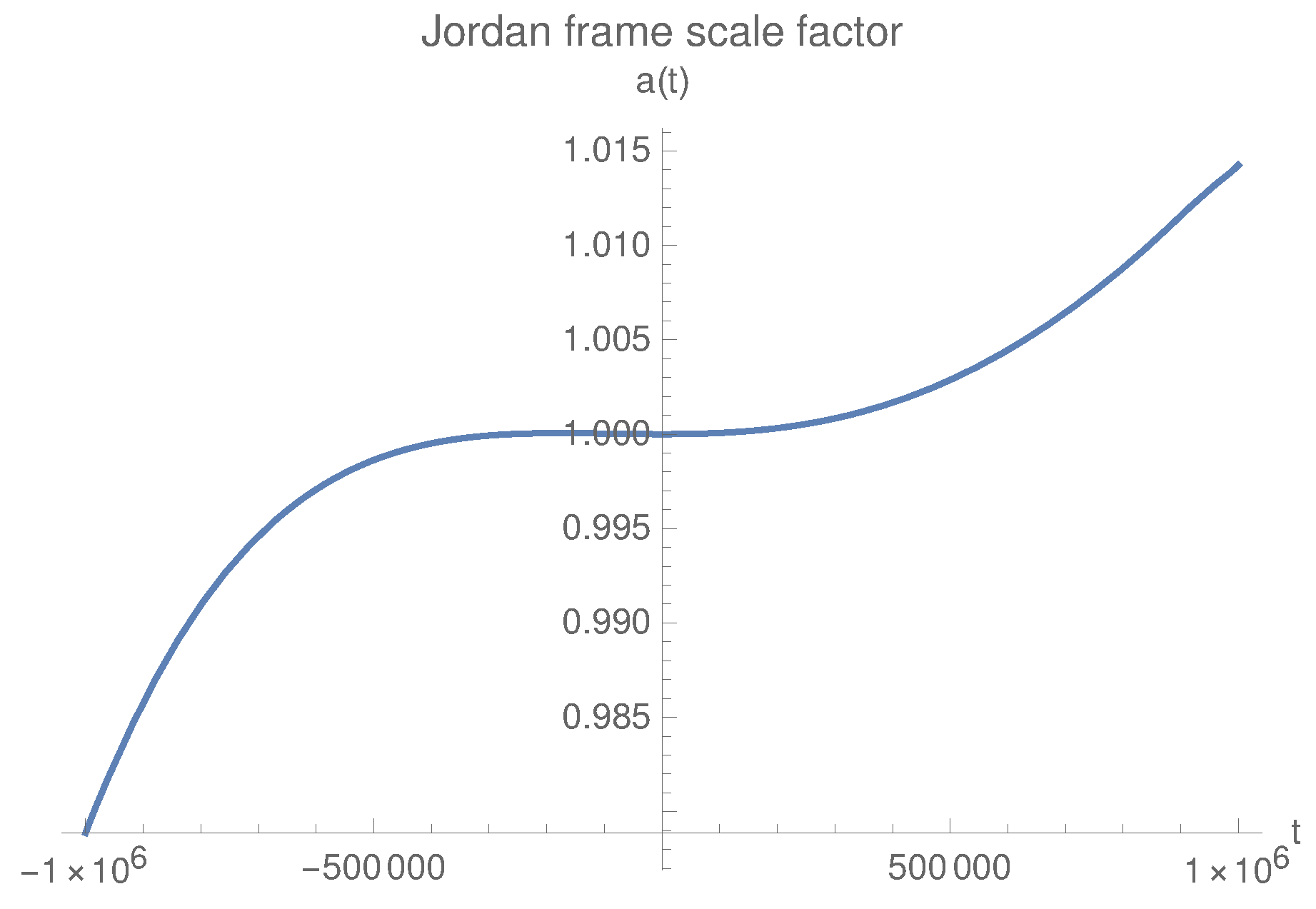
The above statements are in general true for any $f(R)$ theory which accommodates a cosmological bounce. The system behavior, in the particular case of exponential gravity, is shown in the Figure 17, which depicts an universe filled up radiation, and in Figure 18, which depicts the properties of matter less universe. In both the cases we see that the Hubble parameter reaches zero value at two time instants, as predicted from Equation (77). One of the points when the Hubble parameter is zero is placed at $t=0$ where as the other time instant is approximately $-2\times {10}^5$, of the same order as predicted from Equation (77). If one wants to see how the scale-factor of the universe behaves during this period then one can look at Figure 19 and Figure 20. From both the figures one can see that initially the universe was expanding and this expansion slowly stops and a brief period of contraction sets in, the period when the Hubble parameter turns negative, and then this contraction stops slowly and the universe again enters a period of expansion. It is to be noted that if we increase the value of $ϵ$, or $\ddot{H}(0)$ in Jordan frame, then the temporal separation of the two roots in Equation (77) decreases. This implies that the initial expansion phase ends near to the point where later expansion phase starts. In the asymmetric bouncing solutions, as depicted in Figure 4 and Figure 5, in Section 4 we have used non-zero values of $\ddot{H}(0)$ in the Jordan frame, still we are getting perfect bounces and not oscillatory behavior as expected from our present analysis. The reason for this is related to the time period used to study the asymmetric bounces in Section 4 and the specific value of $\ddot{H}(0)$ used there. From the conditions given for the asymmetric bounces one can easily show that the oscillatory behavior should have been evident if we presented the plot for a larger time period. In the time period of interest, only the bouncing region becomes prominent in Figure 4 and Figure 5.

Before we conclude this section we want to show another important property of the new solutions shown. For flat FLRW solutions one can write the Ricci scalar as

$$\begin{array}{c}\hfill R=6(\dot{H}+2H^2)=6(ϵt+b)+12{\left(\frac{ϵt^2}{2}+bt\right)}^2,\end{array}$$

(78)

close to the bounce point. From the above expression one can easily verify that

$$R(0)=6b,R(t=-2b/ϵ)=-6b,$$

which shows that the Ricci scalar has to change sign in between the two temporal values when the Hubble parameter vanishes. As a result of this fact, the universe has to cross the point when $R=0$, between the two expanding regimes. This result is a general result and is true for any $f(R)$ theory which accommodates a cosmological bounce. If we want to work with large, positive values of R and treat $f(R)$ theory as an effective gravitational theory then the new solutions become redundant as only a bounce exists, as analyzed in Section 4. On the other hand if one wants to keep the effect of $f(R)$ bouncing cosmology for very small values of the Ricci scalar, then the new solutions will show up.

8. Conclusions

In this article we presented some early universe solutions coming out from exponential $f(R)$ gravity. The primary reason for choosing exponential gravity is related to the stability of the theory. For positive cosmological constant one always gets $f^{\prime }(R)>0$ and $f^{″}(R)>0$ for all values of R. We presume the theory to be unstable when one moves away from bounce point as in the relevant time limit the Ricci scalar becomes negative and remains unbounded from below. This feature of the theory is well represented in the Einstein frame potential, as shown in Figure 1. We would like to interpret the early universe results, coming out from exponential $f(R)$ theory, as an outcome from some effective theory of gravity which affects in the ultraviolet end.

In this paper we initially present the basics of cosmological dynamics in the two conformal frames, the Jordan frame where the original problem is posed and the Einstein frame which is used to calculate the dynamical development of the system. Our results related to bouncing cosmologies uses two conformal transformations. We show that it is difficult in $f(R)$ theory to have stable bounces. In this regard exponential gravity is an interesting exception as it satisfies the stability conditions for all values as R. In Section 3 we present the bouncing condition in the Jordan frame and its corresponding condition in the Einstein frame. We want to specify here that in spatially flat FLRW spacetimes one in general does not get a simultaneous bounce in both the conformal frames when matter in Jordan frame satisfies $\rho +P\ge 0$ [17]. The conditions of bounce in Jordan frame, when written down in the Einstein frame, shows that the conditions depend upon the second time derivative of the Jordan frame Hubble parameter. Consequently, the bouncing intermediate conditions actually involves the values of all the relevant time derivatives of H in the Jordan frame. It is to be noted that unlike $f(R)$ theories, GR-based cosmology does not require the specification of $\ddot{H}$ at any instant of time. In this article we point out specifically how $\ddot{H}$ can affect cosmological dynamics in higher derivative gravity theory. The evolution of scalar metric perturbations through bounce is presented in Section 5. The whole analysis is done in the Jordan frame and it is shown that the perturbations do not attain any singularity at the bounce point although there me be some modes which can become non-perturbative very near the bounce point. The reason for such non-perturbative evolution may be related to the behavior of curvature related terms near the bounce point. A thorough analysis of stability of metric perturbations in $f(R)$ cosmology, near bounce, is not yet present we hope the theory will be formulated in the near future. We also briefly opine on the fate of the tensor-to-scalar ratio in our $f(R)$ theory induced bounce. We do not expect the present theory to amplify the ratio compared to its value in the prebounce phase.

In the article we present the bouncing solutions in the Jordan frame. In the bouncing solution calculations we use the Einstein frame as an auxiliary frame where the main calculation is done and then we transport the solutions in the Jordan frame via a conformal transformation. The bouncing solutions presented in this paper involve both bounce in vacuum and bounce in the presence of hydrodynamic matter. The examples involve both symmetric and asymmetric bounces. The asymmetry of the bounces is related to finite values of $\ddot{H}(0)$ in the Jordan frame. For symmetric bounces $\ddot{H}(0)=0$. The solutions presented in Section 4 are computed numerically and they are well behaved in our time period of interest, $-{10}^5\le t\le {10}^5$. Outside the time window the solutions can show other features. All the bounces concerned in Section 4 involves variation of positive values of the Ricci scalar in the Jordan frame. Treated $f(R)$ theory as an effective theory of gravity, the exponential gravity bounces become more plausible at higher positive values of R. As exponential gravity becomes similar to GR with positive cosmological constant for low R values one may like to infer that GR effects becomes stronger as R nears zero. The exact turn over from $f(R)$ to GR may involve new physics and is beyond the scope of this paper.

Another interesting property of exponential gravity, as discussed in the paper, is the existence of exact solutions. We present two such solutions in the article. One exact solution is a bouncing solution where the scale-factor of the universe is given by an exponential function of the square of Jordan frame time. This solution can be realized in an universe with matter having positive energy density and equation of state as $-4/3$. With an equation of state lesser than $-1$, the matter does not satisfy $\rho +P\ge 0$ in the Jordan frame and consequently for such an universe one may expect simultaneous bounces in both the Jordan frame and the Einstein frame. The other exact solution is the exponential expansion solution with constant H at a de Sitter point. In vacuum, exponential gravity allows such a solution to exist. One can easily show that such a de-Sitter point exists because exponential gravity involves a positive cosmological constant. If the form of $f(R)$ is suitably changed such that it does not contain any cosmological constant the de-Sitter point vanishes. Using the techniques of dynamical systems we have shown that a constant Hubble parameter solution at the de-Sitter point in exponential gravity is an unstable solution. In effect it is a saddle point solution in the phase space of suitable defined dimensionless phase space variables. We do not present the dynamical system approach in the other solutions in this paper because all the other solutions involve the values $H=0$ and the phase space variables in our analysis always have the Hubble parameter in the denominator. We hope to construct a suitable dynamical systems approach to tackle bouncing problems in the near future.

We present a new solution in $f(R)$ gravity theory in the penultimate section. The new solution in $f(R)$ theories are allowed only if the theory is allowed to be unmodified in the low R regime. As our theory is stable it can safely be extended to the low R regime. The only cost one has to pay to attain these new solutions is that one has to reject the point of view that $f(R)$ gravity is an ultraviolet modification of GR effects. The new results are related to non-zero values of $\ddot{H}(0)$ in the Jordan frame when the other bouncing conditions hold. In such a case one can a have a solution which represent decelerated expansion of the universe in the past. At some point in the past the decelerated expansion comes to a halt momentarily and contraction of the universe starts. This contraction does not lead to a spacetime singularity. In time this contraction slows down and the universe comes to a static configuration momentarily after which again the universe starts to expand. This solution is practically not a bouncing solution, although one can get this solution with an extra intermediate condition on top of the bouncing conditions at $t=0$. The new result which we obtain in this paper is a general result in $f(R)$ gravity which accommodates a bounce. We explicitly show the nature of the solutions in exponential gravity.

References

- Kragh, H. Cyclic models of the relativistic universe: The early history. Einstein Stud. 2018, 14, 183–204. [Google Scholar]
- Guth, A.H. The Inflationary Universe: A Possible Solution to the Horizon and Flatness Problems. Phys. Rev. D 1981, 23, 347–356. [Google Scholar] [CrossRef]
- Linde, A.D. A New Inflationary Universe Scenario: A Possible Solution of the Horizon, Flatness, Homogeneity, Isotropy and Primordial Monopole Problems. Phys. Lett. B 1982, 108, 389–393. [Google Scholar] [CrossRef]
- Martin, J.; Ringeval, C.; Vennin, V. Encyclopædia Inflationaris. Phys. Dark Univ. 2014, 5–6, 75–235. [Google Scholar] [CrossRef]
- Borde, A.; Vilenkin, A. Singularities in inflationary cosmology: A Review. Int. J. Mod. Phys. D 1996, 5, 813–824. [Google Scholar] [CrossRef]
- Novello, M.; Bergliaffa, S.E.P. Bouncing Cosmologies. Phys. Rep. 2008, 463, 127–213. [Google Scholar] [CrossRef]
- Battefeld, D.; Peter, P. A Critical Review of Classical Bouncing Cosmologies. Phys. Rep. 2015, 571, 1–66. [Google Scholar] [CrossRef]
- Buchbinder, I.L.; Odintsov, S.D.; Shapiro, I.L. Effective Action in Quantum Gravity; IOP: Bristol, UK, 1992; 413p. [Google Scholar]
- Vilkovisky, G.A. Effective action in quantum gravity. Class. Quantum Gravity 1992, 9, 895. [Google Scholar] [CrossRef]
- Sotiriou, T.P.; Faraoni, V. f(R) Theories Of Gravity. Rev. Mod. Phys. 2010, 82, 451. [Google Scholar] [CrossRef]
- De Felice, A.; Tsujikawa, S. f(R) theories. Living Rev. Relativ. 2010, 13, 3. [Google Scholar] [CrossRef] [PubMed]
- Nojiri, S.; Odintsov, S.D.; Oikonomou, V.K. Modified Gravity Theories on a Nutshell: Inflation, Bounce and Late-time Evolution. Phys. Rep. 2017, 692, 1–104. [Google Scholar] [CrossRef]
- Nojiri, S.; Odintsov, S.D. Unified cosmic history in modified gravity: From F(R) theory to Lorentz non-invariant models. Phys. Rep. 2011, 505, 59–144. [Google Scholar] [CrossRef]
- Ruzmaikina, T.; Ruzmaikin, A. Quadratic Corrections to the Lagrangian Density of the Gravitational Field and the Singularity. Sov. Phys. J. Exp. Theor. Phys. 1970, 30, 372. [Google Scholar]
- Cai, Y.F.; Saridakis, E.N. Non-singular Cyclic Cosmology without Phantom Menace. J. Cosmol. 2011, 17, 7238–7254. [Google Scholar]
- Saridakis, E.N.; Banerjee, S.; Myrzakulov, R. Bounce and cyclic cosmology in new gravitational scalar-tensor theories. Phys. Rev. D 2018, 98, 063513. [Google Scholar] [CrossRef]
- Paul, N.; Chakrabarty, S.N.; Bhattacharya, K. Cosmological bounces in spatially flat FRW spacetimes in metric f(R) gravity. J. Cosmol. Astropart. Phys. 2014, 2014, 009. [Google Scholar] [CrossRef]
- Bhattacharya, K.; Chakrabarty, S. Intricacies of Cosmological bounce in polynomial metric f(R) gravity for flat FLRW spacetime. J. Cosmol. Astropart. Phys. 2016, 2016, 030. [Google Scholar] [CrossRef]
- Bamba, K.; Makarenko, A.N.; Myagky, A.N.; Nojiri, S.; Odintsov, S.D. Bounce cosmology from F(R) gravity and F(R) bigravity. J. Cosmol. Astropart. Phys. 2014, 2014, 008. [Google Scholar] [CrossRef]
- Carloni, S.; Dunsby, P.K.S.; Solomons, D.M. Bounce conditions in f(R) cosmologies. Class. Quantum Gravity 2006, 23, 1913–1922. [Google Scholar] [CrossRef]
- Elizalde, E.; Nojiri, S.; Odintsov, S.D.; Sebastiani, L.; Zerbini, S. Non-singular exponential gravity: A simple theory for early- and late-time accelerated expansion. Phys. Rev. D 2011, 83, 086006. [Google Scholar] [CrossRef]
- Oikonomou, V.K. Exponential Inflation with F(R) Gravity. Phys. Rev. D 2018, 97, 064001. [Google Scholar] [CrossRef]
- Oikonomou, V.K. An Exponential F(R) Dark Energy Model. Gen. Relativ. Gravit. 2013, 45, 2467–2481. [Google Scholar] [CrossRef]
- Cai, Y.F.; Marciano, A.; Wang, D.G.; Wilson-Ewing, E. Bouncing cosmologies with dark matter and dark energy. Universe 2016, 3, 1. [Google Scholar] [CrossRef]
- Cai, Y.F. Exploring Bouncing Cosmologies with Cosmological Surveys. Sci. China Phys. Mech. Astron. 2014, 57, 1414–1430. [Google Scholar] [CrossRef]
- Barrow, J.D.; Cotsakis, S. Inflation and the Conformal Structure of Higher Order Gravity Theories. Phys. Lett. B 1988, 214, 515–518. [Google Scholar] [CrossRef]
- Matsumoto, J. Cosmological perturbations in F(R) gravity. Phys. Rev. D 2013, 87, 104002. [Google Scholar] [CrossRef]
- Cai, Y.F.; Easson, D.A.; Brandenberger, R. Towards a Nonsingular Bouncing Cosmology. J. Cosmol. Astropart. Phys. 2012, 2012, 020. [Google Scholar] [CrossRef]
- Kobayashi, T. Generic instabilities of nonsingular cosmologies in Horndeski theory: A no-go theorem. Phys. Rev. D 2016, 94, 043511. [Google Scholar] [CrossRef] [Green Version]
- Cai, Y.; Wan, Y.; Li, H.G.; Qiu, T.; Piao, Y.S. The Effective Field Theory of nonsingular cosmology. J. High Energy Phys. 2017, 2017, 090. [Google Scholar] [CrossRef]
- Raveendran, R.N.; Chowdhury, D.; Sriramkumar, L. Viable tensor-to-scalar ratio in a symmetric matter bounce. J. Cosmol. Astropart. Phys. 2018, 2018, 030. [Google Scholar] [CrossRef]
- Odintsov, S.D.; Sá¡ez-Chillán Gámez, D.; Sharov, G.S. Is exponential gravity a viable description for the whole cosmological history? Eur. Phys. J. C 2017, 77, 862. [Google Scholar] [CrossRef] [PubMed] [Green Version]
- Schmidt, H.J. Exact cosmological solutions of nonlinear F(R) gravity. arXiv, 1998; arXiv:gr-qc/9808060. [Google Scholar]
- Wei, H.; Li, H.Y.; Zou, X.B. Exact cosmological solutions of f(R) theories via Hojman symmetry. Nucl. Phys. B 2016, 903, 132–149. [Google Scholar] [CrossRef]
- Bari, P.; Bari, P.; Chakraborty, S.; Bhattacharya, K. Causal horizons in a bouncing universe. Gen. Relat. Gravit. 2018, 50, 118. [Google Scholar] [CrossRef]
- Amendola, L.; Gannouji, R.; Polarski, D.; Tsujikawa, S. Conditions for the cosmological viability of f(R) dark energy models. Phys. Rev. D 2007, 75, 083504. [Google Scholar] [CrossRef]
- Carloni, S.; Troisi, A.; Dunsby, P.K.S. Some remarks on the dynamical systems approach to fourth order gravity. Gen. Relat. Gravit. 2009, 41, 1757–1776. [Google Scholar] [CrossRef] [Green Version]
- Carloni, S.; Dunsby, P.K.S.; Capozziello, S.; Troisi, A. Cosmological dynamics of R**n gravity. Class. Quantum Gravity 2005, 22, 4839–4868. [Google Scholar] [CrossRef]
- Odintsov, S.D.; Oikonomou, V.K. Autonomous dynamical system approach for f(R) gravity. Phys. Rev. D 2017, 96, 104049. [Google Scholar] [CrossRef]