Quantum Gravity at the Corner

Abstract

We investigate the quantum geometry of a 2d surface S bounding the Cauchy slices of a 4d gravitational system. We investigate in detail for the first time the boundary symplectic current that naturally arises in the first-order formulation of general relativity in terms of the Ashtekar–Barbero connection. This current is proportional to the simplest quadratic form constructed out of the pull back to S of the triad field. We show that the would-be-gauge degrees of freedo arising from $SU(2)$ gauge transformations plus diffeomorphisms tangent to the boundary are entirely described by the boundary 2-dimensional symplectic form, and give rise to a representation at each point of S of $SL(2,\mathbb{R})\times SU(2)$. Independently of the connection with gravity, this system is very simple and rich at the quantum level, with possible connections with conformal field theory in 2d. A direct application of the quantum theory is modelling of the black horizons in quantum gravity.

1. Introduction

In the construction of black hole models in loop quantum gravity [1,2,3] via the so-called isolated horizon boundary condition [4], the boundary would-be-gauge degrees of freedom are described by a Chern–Simons theory living on the black hole horizon [5,6,7,8]. The appearance of the specific Chern–Simons boundary dynamics is usually argued to be due to restrictions on the set of boundary conditions adapted to isolated horizons. What we realise here is that the appearance of a boundary dynamical theory and the appearance of a boundary symplectic structure is not specific to black holes, and arises naturally in the most general situation [9]. As we explain, the general boundary dynamics can be understood in terms of a Chern–Simons theory. However, this Chern–Simons theory does not need the introduction of auxiliary fields. Remarkably, it can be expressed very simply in terms of the pull back of the triad frame field on the boundary, while the pull back of the spin connection acts as a Lagrange multiplier for the boundary diffeomorphisms. The boundary symplectic structure is remarkably simple. It reads

$$\mathsf{\Theta }=\frac{1}{2\gamma }{\int }_{\partial \mathsf{\Sigma }}\delta e^i\wedge \delta e_i,$$

(1)

where $\gamma$ is the Immirzi parameter and $e^i$ the triad field pull back on the 2d boundary of the slice $\mathsf{\Sigma }$. This remarkably simple and natural boundary structure constitutes one of the central building blocks of first-order gravity theory projected on any corner sphere.

In this paper, we provide detailed proof that the symplectic structure (1) allows a complete Hamiltonian description of the boundary gauge diffeomorphism transformations. This shows that these would-be-gauge degrees of freedom exhaust the set of boundary degrees of freedom. This symplectic structure first made its appearance in [7] (see also [10] for a discussion in higher dimension), but its central importance was not emphasised and it was not studied in full generality. At first sight, such theory would seem harder to quantise, as the standard techniques developed for the background independent quantisation of connections cannot be directly applied. However, quantisation is made possible by the choice of a complex structure on the 2-dimensional boundary associated with fiducial coordinates. This leads to expressing the triad in terms of harmonic oscillators associated to point defects (punctures) on the boundary. The unrestricted Hilbert space is much larger than the one found for quantum isolated horizons, as expected from the fact that no classical symmetry reduction on the geometry of the boundary has been imposed. We show that the representations of the geometric observables can be constrained in a simple way in order to recover the usual accounts of black hole entropy in the literature.

The paper is organised as follows. In the following section, we describe the geometric context in which the 2-dimensional model we analyse is natural. We also show how in the situations where $SU\left(2\right)$ gauge transformations and bulk diffeomorphisms that are tangent to the boundary are gauge symmetries of gravity. In Section 3, we analyse the boundary symplectic structure and define the associated three-dimensional theory encoding the entire dynamics of the would-be-gauge degrees of freedom is controlled by our $2+1$-dimensional system. In Section 4 we quantise the system and interpret the states in terms of the underlying complex structure. We close the paper with some concluding remarks in relation to the applicability of our results for the computation of black hole entropy in Section 5.

2. The Origin of the 2d Symplectic Structure

Starting from the first-order formulation of gravity whose action is

$$S[e,\omega ]={\int }_M{ϵ}_{IJKL}{e}^I\wedge e^K\wedge F^{KL}(\omega ),$$

(2)

introducing a foliation of M in terms of Cauchy surfaces $\mathsf{\Sigma }$, and using the time gauge $e^0=n$ where n is the co-normal to $\mathsf{\Sigma }$, the canonical symplectic structure of gravity takes the form

$${\mathsf{\Omega }}_C={\int }_{\mathsf{\Sigma }}\delta K^i\wedge \delta {\mathsf{\Sigma }}_i,$$

(3)

where $K^i\equiv {\omega }^{0i}$ is the extrinsic curvature one-form and $\mathsf{\Sigma }=\frac{1}{2}{ϵ}_{ijk}{e}^j\wedge e^k$ is the flux two-form. Here and in the following, $\delta$ denotes the differential on field space, in particular as a differential it anti-commutes with itself and its square ${\delta }^2=0$ vanishes. It should not be confused with $\mathrm{d}$, which denotes the differential on space. The symplectic form in Ashtekar–Barbero variables is given by

$$\mathsf{\Omega }\equiv \frac{1}{\gamma }{\int }_{\mathsf{\Sigma }}\delta A^i\wedge \delta {\mathsf{\Sigma }}_i,$$

(4)

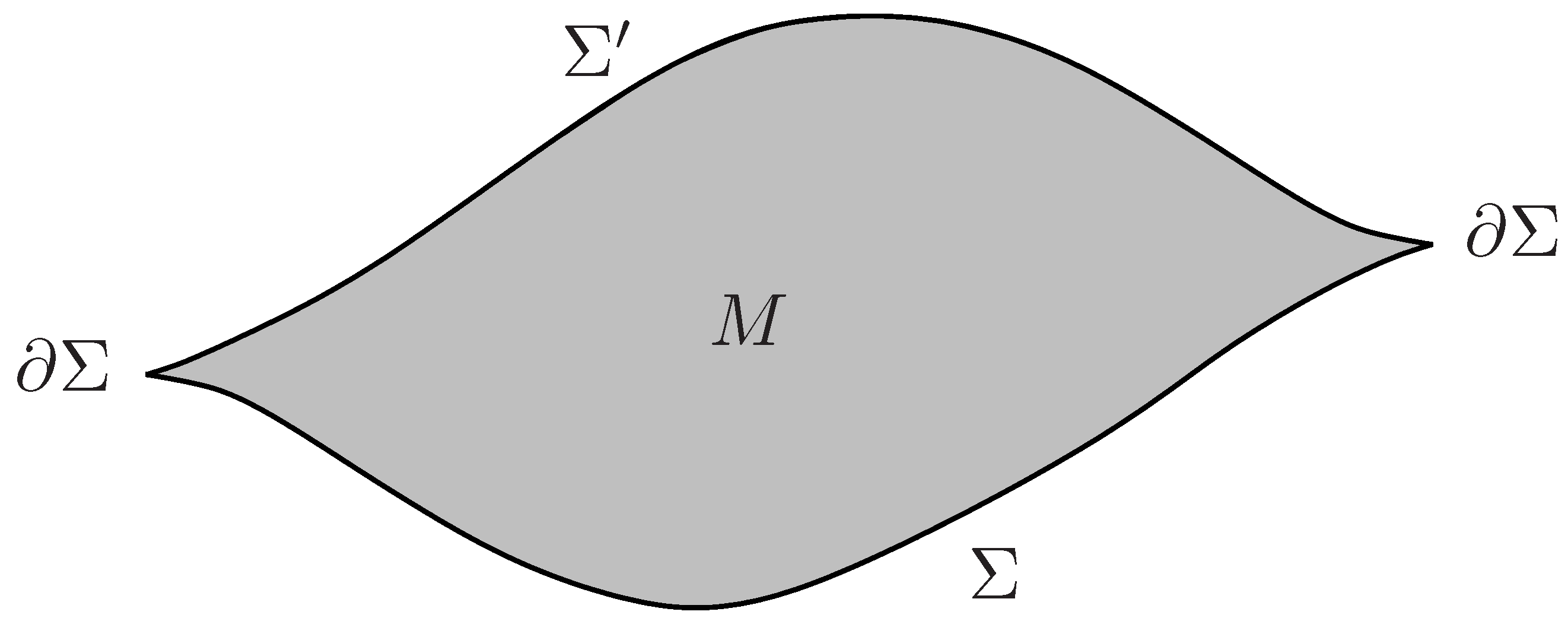
where $A^i$ is the $SU(2)$ connection, which can be expressed as $A^i={\mathsf{\Gamma }}^i+\gamma K^i$, in terms of the spin connection ${\mathsf{\Gamma }}^i\equiv \frac{1}{2}{{ϵ}^i}_{jk}{\omega }^{jk}$ and the extrinsic curvature tensor $K^i\equiv {\omega }^{0i}$ with ${\omega }^{IJ}$ the Lorentz connection. In the absence of boundaries, one has that $\mathsf{\Omega }={\mathsf{\Omega }}_C$, and this is the celebrated result allowing to interpret the previous connection as a canonical transformation from the original vector variables [11,12]. In the presence of a boundary $\partial \mathsf{\Sigma }\ne 0$ (see Figure 1), one has that

$${\mathsf{\Omega }}_C=\mathsf{\Omega }+\mathsf{\Theta },$$

(5)

where $\mathsf{\Theta }$ is the boundary symplectic structure given by [7]

$$\mathsf{\Theta }\equiv \frac{1}{2\gamma }{\int }_{\partial \mathsf{\Sigma }}\delta e^i\wedge \delta e_i,$$

(6)

as it follows from

$$\mathsf{\Theta }=-\gamma {\int }_{\mathsf{\Sigma }}\delta {\mathsf{\Gamma }}^i\wedge \delta {[e,e]}_i=\frac{1}{2\gamma }{\int }_{\mathsf{\Sigma }}\mathrm{d}(\delta e_i\wedge \delta e^i),$$

(7)

and from the identification

$${\mathsf{\Sigma }}_i=\frac{1}{2}{[e,e]}_i,$$

(8)

which is valid at the boundary.

Figure 1. Spacetime region obtained from the time flow that is allowed in our analysis. Lapse and shift are constrained on the corners $\partial \mathsf{\Sigma }$ in order to preserve the boundary fixed up to tangent diffeomorphisms and gauge transformations.

Therefore, in the context of Ashtekar–Barbero variables, the boundary term (1) arises naturally from the (pseudo) canonical transformation that relates (3) and (4) in the absence of boundaries. The transformation is pseudo-canonical because when there are boundaries Equation (7) produces a boundary corner term (1) in the symplectic structure. This corresponds exactly to one of the intrinsic ambiguities in the determination of the symplectic structure from an action principle [13]. The symplectic potential $\theta$ is defined from the boundary terms arising in the variations of the action, but they are subjected to the following ambiguities:

$$\theta \to \theta +\delta {\mu }_1+d{\mu }_2,$$

(9)

where ${\mu }_1$ arises from the possibility of modifying the action by the addition of an exact four-form to the Lagrangian form, and ${\mu }_2$ is an arbitrary corner term. No general principle fixes ${\mu }_2$. However, in our present specific context ${\mu }_2$ is singled out by the use of connection variables—Equation (7)—and the fact that it leads to the correct evaluation of boundary charges and the commutation relations that are compatible with the kinematics of LQG.

2.1. Symmetries

In this section we analyse the transformation property of the symplectic form $\mathsf{\Omega }+\mathsf{\Theta }$ under two types of transformation: $SU(2)$ gauge transformations labelled by $\alpha \in \mathfrak{su}(2)$, and spatial diffeomorphism labelled by a vector field $\xi$. Our variables are the bulk variables $({\mathsf{\Sigma }}_i,A^i)$: a Lie algebra valued two-form and an $SU(2)$ connection on $\mathsf{\Sigma }$; and the boundary variables $e_i$, which is a Lie algebra valued one-form on $\partial \mathsf{\Sigma }$. We initially treat these variables as independent variables. As we will see, the gauge symmetry will restore the relationship (8) at the boundary.

The gauge transformations are labelled by an $SU(2)$ Lie algebra element ${\alpha }^i$, and are defined to be

$${\delta }_{\alpha }A\equiv -{\mathrm{d}}_A\alpha ,{\delta }_{\alpha }\mathsf{\Sigma }\equiv [\alpha ,\mathsf{\Sigma }],{\delta }_{\alpha }{e}_i\equiv [\alpha ,e].$$

(10)

Infinitesimal diffeomorphisms are labelled by a vector field $\xi$ and generated by the Lie derivative

$${\mathcal{L}}_{\xi }\equiv \mathrm{d}{i}_{\xi }+i_{\xi }\mathrm{d},$$

(11)

where $i_{\xi }{T}_{bc\cdots d}\equiv {\xi }^a{T}_{abc\cdots d}+{\xi }^a{T}_{bac\cdots d}+\cdots$ is the inner contraction for an arbitrary tensor $T_{abc\cdots d}$. This Lie derivative has the disadvantage of not preserving the $SU(2)$ covariance when acting on $SU(2)$ tensors, since it does not commute with gauge transformations $[{\mathcal{L}}_{\xi },{\delta }_{\alpha }]\ne 0$. For that reason, it is more natural to work with a gauge-invariant Lie derivative denoted $L_{\xi }$ which preserves the covariance under gauge transformations: $[L_{\xi },{\delta }_{\alpha }]=0$ (the previous relation is valid when applied to covariant tensors). This covariant Lie derivative acts on SU(2) tensors like $e_i$ or ${\mathsf{\Sigma }}_i$ or $F^i(A)$ as

$$L_{\xi }\equiv {\mathrm{d}}_A{i}_{\xi }+i_{\xi }{\mathrm{d}}_A,$$

(12)

but it acts differently on the gauge connection1 since

$$L_{\xi }A\equiv i_{\xi }F(A).$$

(13)

This covariant Lie derivative restricts to the usual Lie derivative for $SU(2)$ scalars. On $SU(2)$ tensors, the covariant and usual Lie derivative are equivalent up to gauge transformations. The relation is simply

$$L_{\xi }={\mathcal{L}}_{\xi }+{\delta }_{i_{\xi }A}.$$

(14)

In the following, we use $L_{\xi }$ as the generator of covariant diffeomorphisms. $\xi$ is a vector field on $\mathsf{\Sigma }$ which is assumed to be tangent to $\partial \mathsf{\Sigma }$. Therefore, $\xi$ labels an infinitesimal diffeomorphism of $\mathsf{\Sigma }$ which does not move the boundary.

2.2. Hamiltonian Generators

The goal of this section is to show that the Hamiltonian generators of covariant diffeomorphisms $L_{\xi }$ and gauge symmetry ${\delta }_{\alpha }$ are given by

$$H_{\xi }\equiv {\int }_{\mathsf{\Sigma }}{i}_{\xi }F\wedge \mathsf{\Sigma }+\frac{1}{2}{\int }_{\partial \mathsf{\Sigma }}{L}_{\xi }{e}^i\wedge e_i,G_{\alpha }\equiv -{\int }_{\mathsf{\Sigma }}{\mathrm{d}}_A{\alpha }^i\wedge {\mathsf{\Sigma }}_i+\frac{1}{2}{\int }_{\partial \mathsf{\Sigma }}{\alpha }_i{[e,e]}^i.$$

(15)

We start by computing the variation of the gauge Hamiltonian.

$$\begin{array}{cc}\hfill \delta G_{\alpha }& =-{\int }_{\mathsf{\Sigma }}{\mathrm{d}}_A{\alpha }_i\wedge \delta {\mathsf{\Sigma }}^i-{\int }_{\mathsf{\Sigma }}\delta A^i\wedge {[\alpha ,\mathsf{\Sigma }]}_i+{\int }_{\partial \mathsf{\Sigma }}{[\alpha ,e]}^i\wedge \delta e_i\hfill \\ & ={\int }_{\mathsf{\Sigma }}{\delta }_{\alpha }{A}_i\wedge \delta {\mathsf{\Sigma }}^i-{\int }_{\mathsf{\Sigma }}\delta A_i\wedge {\delta }_{\alpha }{\mathsf{\Sigma }}^i+{\int }_{\partial \mathsf{\Sigma }}{\delta }_{\alpha }{e}^i\wedge \delta e_i\hfill \\ & =\gamma {\delta }_{\alpha }⌟(\mathsf{\Omega }+\mathsf{\Theta }),\hfill \end{array}$$

(16)

where ${\delta }_{\alpha }⌟\mathsf{\Omega }$ denotes the interior product of the field variation ${\delta }_{\alpha }$ with the field two-form $\mathsf{\Omega }+\mathsf{\Theta }$. This shows that $G_{\alpha }$ is the Hamiltonian generating $SU(2)$ gauge transformations. This generator is the sum of a bulk and a boundary terms. The bulk constraint imposes the Gauss law while the boundary constraints impose a soldering of the boundary degree of freedom to the bulk degree of freedom. Integrating by parts, we can write

$$G_{\alpha }={\int }_{\mathsf{\Sigma }}{\alpha }^i\wedge {\mathrm{d}}_A{\mathsf{\Sigma }}_i+{\int }_{\partial \mathsf{\Sigma }}{\alpha }_i\left(\frac{1}{2}{[e,e]}^i-{\mathsf{\Sigma }}^i\right).$$

(17)

In short, $G_{\alpha }=0$ means that

$${\mathrm{d}}_A{\mathsf{\Sigma }}_i=0,{\mathsf{\Sigma }}_i=\frac{1}{2}{[e,e]}_i.$$

(18)

The first condition is the usual Gauss law. The second one is a first-class boundary constraint simply demanding that the induced area density from the bulk and the intrinsic one match2.

It is convenient to introduce the boundary variation and Hamiltonian:

$${\delta }_{\alpha }{e}^i\equiv {[\alpha ,e]}^i,g_{\alpha }\equiv {\int }_{\partial \mathsf{\Sigma }}2{\alpha }_i{[e,e]}^i.$$

(19)

$g_{\alpha }$ is the generator of boundary variations. It does not act on the bulk fields but is the Hamiltonian for boundary rotations:

$$\begin{array}{c}\hfill \delta g_{\alpha }={\int }_{\partial \mathsf{\Sigma }}{[\alpha ,e]}^i\wedge \delta e_i=\gamma {\delta }_{\alpha }⌟\mathsf{\Theta }.\end{array}$$

(20)

We now do the same computation for the diffeomorphism variation. This computation is more involved, and in order to do it we separate the bulk and boundary variations. We start with

$$\begin{array}{cc}\hfill \delta \left({\int }_{\mathsf{\Sigma }}{i}_{\xi }{F}_i\wedge {\mathsf{\Sigma }}^i\right)& ={\int }_{\mathsf{\Sigma }}{i}_{\xi }{\mathrm{d}}_A\delta A_i\wedge {\mathsf{\Sigma }}^i+{\int }_{\mathsf{\Sigma }}{i}_{\xi }{F}^i\wedge \delta {\mathsf{\Sigma }}_i\hfill \\ & =-{\int }_{\mathsf{\Sigma }}{\mathrm{d}}_A\delta A_i\wedge i_{\xi }{\mathsf{\Sigma }}^i+{\int }_{\mathsf{\Sigma }}{i}_{\xi }{F}^i\wedge \delta {\mathsf{\Sigma }}_i\hfill \\ & =-{\int }_{\partial \mathsf{\Sigma }}\delta A_i\wedge i_{\xi }{\mathsf{\Sigma }}^i+{\int }_{\mathsf{\Sigma }}{i}_{\xi }{F}^i\wedge \delta {\mathsf{\Sigma }}_i-{\int }_{\mathsf{\Sigma }}\delta A_i\wedge {\mathrm{d}}_A\left(i_{\xi }{\mathsf{\Sigma }}^i\right)\hfill \\ & ={\int }_{\partial \mathsf{\Sigma }}{i}_{\xi }\left(\delta A_i\wedge {\mathsf{\Sigma }}^i\right)+{\int }_{\mathsf{\Sigma }}{i}_{\xi }{F}^i\wedge \delta {\mathsf{\Sigma }}_i-{\int }_{\mathsf{\Sigma }}\delta A_i\wedge L_{\xi }{\mathsf{\Sigma }}^i-{\int }_{\mathsf{\Sigma }}\delta A_i\wedge i_{\xi }\left({\mathrm{d}}_A{\mathsf{\Sigma }}^i\right)-{\int }_{\partial \mathsf{\Sigma }}\left(i_{\xi }\delta A_i\right)\wedge {\mathsf{\Sigma }}^i\hfill \\ & ={\int }_{\partial \mathsf{\Sigma }}{i}_{\xi }\left(\delta A_i\wedge {\mathsf{\Sigma }}^i\right)+\gamma {\delta }_{\xi }⌟\mathsf{\Omega }+G_{\left(i_{\xi }\delta A\right)}-g_{\left(i_{\xi }\delta A\right)}\hfill \\ & =\gamma L_{\xi }⌟\mathsf{\Omega }+G_{\left(i_{\xi }\delta A\right)}-g_{\left(i_{\xi }\delta A\right)},\hfill \end{array}$$

(21)

where on the last line we used that ${\xi |}_{\partial \mathsf{\Sigma }}$ is a vector tangent to $\partial \mathsf{\Sigma }$. We can now focus on the boundary term variation. We define the boundary Hamiltonian

$$h_{\xi }\equiv \frac{1}{2}{\int }_{\partial \mathsf{\Sigma }}{L}_{\xi }{e}_i\wedge e^i.$$

(22)

Its variation is given by

$$\begin{array}{cc}\hfill \delta h_{\xi }& =\frac{1}{2}{\int }_{\partial \mathsf{\Sigma }}[\left(i_{\xi }\delta A\right),e_i]\wedge e^i+\frac{1}{2}{\int }_{\partial \mathsf{\Sigma }}{L}_{\xi }\delta e_i\wedge e^i+\frac{1}{2}{\int }_{\partial \mathsf{\Sigma }}{L}_{\xi }{e}_i\wedge \delta e^i\hfill \\ & ={\int }_{\partial \mathsf{\Sigma }}\left(i_{\xi }\delta A_i\right)\wedge \frac{1}{2}{[e,e]}^i+\frac{1}{2}{\int }_{\partial \mathsf{\Sigma }}{L}_{\xi }\left(\delta e_i\wedge e^i\right)+{\int }_{\partial \mathsf{\Sigma }}{L}_{\xi }{e}_i\wedge \delta e^i\hfill \\ & =\frac{1}{2}{\int }_{\partial \mathsf{\Sigma }}{i}_{\xi }\mathrm{d}\left(\delta e_i\wedge e^i\right)+g_{i_{\xi }\delta A}+\gamma L_{\xi }⌟\mathsf{\Theta }\hfill \\ & =\gamma L_{\xi }⌟\mathsf{\Theta }+g_{i_{\xi }\delta A},\hfill \end{array}$$

(23)

where we have assumed again that $\xi$ is a vector tangent to the boundary. Taking the sum of (21) and (23) gives

$$\delta H_{\xi }=\gamma L_{\xi }⌟(\mathsf{\Omega }+\mathsf{\Theta })+G_{i_{\xi }\delta A}.$$

(24)

We can also use the gauge variation, computed already in (16), to establish that

$$\delta G_{i_{\xi }A}=\gamma {\delta }_{i_{\xi }A}⌟(\mathsf{\Omega }+\mathsf{\Theta })+G_{i_{\xi }\delta A}.$$

(25)

This implies that if one introduces the generator of (non-covariant) diffeomorphism $D_{\xi }\equiv H_{\xi }-G_{i_{\xi }A}$. Taking the difference of the previous equalities, one obtains that

$$\delta D_{\xi }=\gamma {\mathcal{L}}_{\xi }⌟(\mathsf{\Omega }+\mathsf{\Theta }).$$

(26)

Imposing the covariant diffeomorphism constraints implies that we impose a bulk and a boundary constraint given by

$$\left(i_{\xi }{F}_i\right)\wedge {\mathsf{\Sigma }}^i=0,h_{\xi }=0.$$

(27)

The boundary constraint can be expressed more explicitly as

$$\begin{array}{cc}\hfill h_{\xi }& =\frac{1}{2}{\int }_{\partial \mathsf{\Sigma }}{\mathrm{d}}_{\mathsf{\Gamma }}\left(i_{\xi }{e}_i\right)\wedge e^i+\frac{\gamma }{2}{\int }_{\partial \mathsf{\Sigma }}\left(i_{\xi }{K}_i\right)\wedge {[e,e]}^i\hfill \end{array}$$

(28)

$$\begin{array}{cc}=& \frac{\gamma }{2}{\int }_{\partial \mathsf{\Sigma }}\left(i_{\xi }{K}_i\right)\wedge {[e,e]}^i=\gamma g_{i_{\xi }K}.\hfill \end{array}$$

(29)

In order to understand the meaning of the condition $h_{\xi }=0$ for all $\xi$ tangent to $\partial \mathsf{\Sigma }$, we now study its geometrical meaning which follows from the following analysis. We can write $K_a^i={\alpha }^{ij}{e}_{ai}$, and the imposition of the Gauss law implies that $K^{ij}$ is a symmetric internal tensor. The extrinsic curvature can be written as $K_{ab}=K_{ij}{e}_a^i{e}_b^j$. We introduce $N_a$ a spatial unit vector, to be the normal of $\partial \mathsf{\Sigma }$ within $\mathsf{\Sigma }$, and we go to the gauge where $e_a^3=N_a$. The condition $h_{\xi }=0$ implies that ${\alpha }^{3A}=0$ for $A=1,2$, which means that the second fundamental form is $K_{ab}={\alpha }_{AB}{e}_a^A{e}_b^B+{\alpha }_{33}{e}_a^3{e}_a^3$, or simply that

$$K_{ab}=k_{ab}+{\alpha }_{33}{N}_a{N}_b,$$

(30)

where $k_{ab}$ is a symmetric tensor tangent to $\partial \mathsf{\Sigma }$ (i.e., $k_{ab}{N}^a=0$). $k_{ab}$ is the 2d extrinsic curvature of $\partial \mathsf{\Sigma }$ as embedded in $\mathsf{\Sigma }$. The 3d extrinsic curvature $K_{ab}$ can be written as $K_{ab}=\frac{1}{3}\theta q_{ab}+{\sigma }_{ab}$, that is, into its trace part (the expansion) $\theta$ and traceless part (the shear) ${\sigma }_{ab}$. The previous expression implies that the shear

$${\sigma }_{ab}={\sigma }_{ab}^{\left(2\right)}+{\sigma }_{33}{N}_a{N}_b,$$

(31)

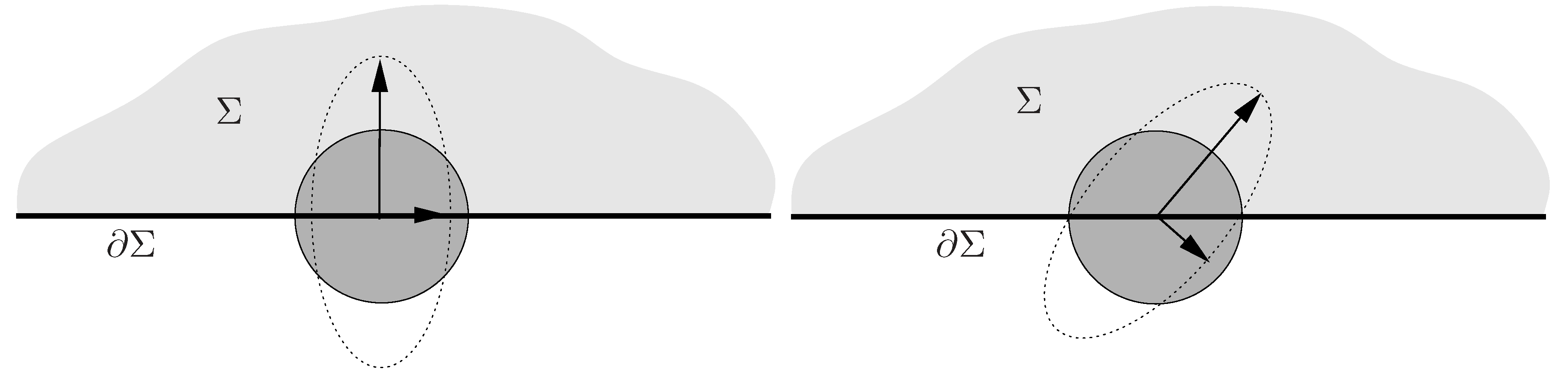
which means that $N_a$ is one of the principal axes of the shear while the other two are tangent to $\partial \mathsf{\Sigma }$. The geometric interpretation is now clear (see Figure 2): an infinitesimal spherical ball around a point at $\partial \mathsf{\Sigma }$ when propagated along the timelike geodesics normal to $\mathsf{\Sigma }$ is allowed to expand and deform along directions which are either normal or tangent to $\partial \mathsf{\Sigma }$. Deformation in an alternative direction is precluded by $h_{\xi }=0$. This can be interpreted as a condition of non-rotation for the boundary $\partial \mathsf{\Sigma }$. In the case when an axisymmetry Killing field $\xi$ tangent to $\partial \mathsf{\Sigma }$ is available, then $h_{\xi }$ is exactly the Komar angular momentum3.

Figure 2. Deformation of a ball of geodesics normal to $\mathsf{\Sigma }$. On the left panel $h_{\xi }=0$: the principal axis of the shear are tangent to $\partial \mathsf{\Sigma }$ and normal to $\partial \mathsf{\Sigma }$. On the right panel $h_{\xi }\ne 0$, the boundary “moves”.

From (24), the Poisson bracket of two Hamiltonians is therefore given by

$$\{H_{\xi },H_{{\xi }^{\prime }}\}=L_{\xi }⌟(L_{{\xi }^{\prime }}⌟(\mathsf{\Omega }+\mathsf{\Theta }))=L_{\xi }{H}_{{\xi }^{\prime }}=H_{[\xi ,{\xi }^{\prime }]}.$$

(33)

Thus, on-shell (i.e., when $i_{\xi }{F}^i\wedge {\mathsf{\Sigma }}_i=0$) the commutation relation of the angular momenta simply gives a representation of the 2-dimensional diffeomorphism algebra:

$$\{h_{\xi },h_{{\xi }^{\prime }}\}\simeq h_{[\xi ,{\xi }^{\prime }]},$$

(34)

where $[\xi ,{\xi }^{\prime }]$ is the Lie-bracket of the two vector fields. Let us finally remember that the boundary generator of diffeomorphism is given by $d_{\xi }=h_{\xi }-g_{i_{\xi }A}$ and explicitly expressed as

$$d_{\xi }=\frac{1}{2}{\int }_{\partial \mathsf{\Sigma }}{\mathcal{L}}_{\xi }{e}_i\wedge e^i.$$

(35)

Non-static boundaries for which $h_{\xi }\ne 0$ are physically very interesting (an important example is the Kerr black hole horizon when treated as a boundary). However, the presence of angular momentum makes the question of diffeomorphism invariance more subtle, and this introduces additional complications when one aims at the quantisation of the boundary would-be-gauge degrees of freedom. For an exploration of the quantisation of a non-static boundary, see [16]. For that reason, in what follows we will restrict ourselves to the static case $h_{\xi }=0$.

3. Boundary Symplectic Structure

The previous section showed that for the set of variation generated by gauge and diffeomorphism, the bulk symplectic structure is equivalent to the boundary symplectic structure

$$\mathsf{\Theta }\equiv \frac{1}{2\gamma }{\int }_H\delta e_i\wedge \delta e^i.$$

(36)

This symplectic structure controls the “would-be-gauge” degrees of freedom. The remarkable property of this symplectic structure is that it leads to a non-commutative flux algebra. Indeed, defining for $S\subset H$

$$X_{\alpha }\left(S\right)\equiv {\int }_S{\mathsf{\Sigma }}_i{\alpha }^i,$$

(37)

we have

$$\{X_{\alpha }\left(S\right),X_{\beta }\left(S^{\prime }\right)\}=\gamma X_{[\alpha ,\beta ]}(S\cup S^{\prime }).$$

(38)

In terms of the components $e_A^i$, the Poisson structure reads

$$\{e_A^i\left(x\right),e_B^j\left(x^{\prime }\right)\}=\gamma {ϵ}_{AB}{\delta }^{ij}{\delta }^2(x-x^{\prime }).$$

(39)

Note that if we define some integrated version of the frame field along curves C: $e_A^i\left(C\right)={\int }_C{e}^i\left(x\right),$ we obtain the loop algebra

$$\{e_A^i\left(C\right),e_B^j\left(C^{\prime }\right)\}=\gamma N_{C\cap C^{\prime }}{ϵ}_{AB}{\delta }^{ij},$$

(40)

where $N_{C\cap C^{\prime }}$ is the number of intersections of C with $C^{\prime }$ with positive orientation minus the number of intersections with negative orientation.

3.1. The Associated Boundary 2 + 1 Dynamical Theory

Here we write a $2+1$ dynamical theory from which the 2d boundary symplectic structure (36) arises in the canonical analysis. In addition, the constraint structure of the theory is compatible with the gauge symmetries expected to be relevant for the boundary degrees of freedom in view of eventually coupling them to the bulk quantum gravitational degrees of freedom of the ambient 3d quantum geometry.

Consider the $2+1$ action on $\partial \mathsf{\Sigma }\times \mathbb{R}$

$$S[{\overline{e}}^i,{\overline{\omega }}^i]=-\frac{1}{\gamma }\int {\overline{e}}_i\wedge (d{\overline{e}}^i+{ϵ}_{ijk}{\overline{\omega }}^j\wedge {\overline{e}}^k).$$

(41)

First-order variations of this action yield the symplectic structure (36) and the equations of motion telling us that ${\overline{\omega }}_i$ is simply a Lagrange multiplier imposing ${\overline{e}}^i\wedge {\overline{e}}^j{ϵ}_{ijk}=0$ and that $d_{\omega }{\overline{e}}^i=0$. There are non-trivial solutions corresponding to degenerate triads. The degeneracy condition demands that $e_a^i$ is a matrix of rank one.

The previous action is the analog of the Chern–Simons action in the effective treatments of [5,6,7]. However, unlike the latter, the present one does have local degrees of freedom, and this will explicitly show up in the quantisation. The present dynamical framework is therefore more general, as expected from the fact that, in contrast to the approach leading to the Chern–Simons formulation, we have not imposed any symmetry restriction on the boundary geometry.

The canonical analysis of (41) yields the Poisson brackets (39). Taking a $2+1$ decomposition ${\overline{e}}_i={\beta }_i\mathrm{d}t+e_i$ and ${\overline{\omega }}^i={\alpha }^i\mathrm{d}t+{\omega }^i$, where the barred forms are 2-dimensional, we find that $S=\int \mathrm{d}tL$, with

$$L=\frac{1}{2\gamma }{\int }_{\partial \mathsf{\Sigma }}{e}^i\wedge {\partial }_t{e}_i-\frac{1}{\gamma }{\int }_{\partial \mathsf{\Sigma }}{\alpha }_i{[e,e]}^i+{\beta }_i{\mathrm{d}}_{\omega }{e}^i+{\gamma }_i{\mathsf{\Pi }}_{\omega }^i,$$

(42)

where ${\mathsf{\Pi }}_{\omega }$ is the momentum conjugate to $\omega$. The Hamiltonian is a linear combination of primary constraints:

$$\begin{array}{c}\hfill g\left(\alpha \right)={\int }_{\partial \mathsf{\Sigma }}{\alpha }_i{[e,e]}^i,d\left(\beta \right)={\int }_{\partial \mathsf{\Sigma }}{\beta }^i{\mathrm{d}}_{\omega }{e}_i\mathsf{\Pi }\left(\gamma \right)={\int }_{\partial \mathsf{\Sigma }}{\gamma }_i{\mathsf{\Pi }}_{\omega }^i.\end{array}$$

(43)

The first is the Gauss law that implies that $e_i$ is degenerate, while the second implies that $e^i$ is $\omega$-closed. The requirement that ${\mathsf{\Pi }}_{\omega }$ is preserved by time evolution implies that

$${[\beta ,e]}^i=0.$$

(44)

This condition reduces the constraint system to the following first-class system:

$$\begin{array}{c}\hfill g\left(\alpha \right)={\int }_{\partial \mathsf{\Sigma }}{\alpha }_i{[e,e]}^i,d\left(\beta \right)={\int }_{\partial \mathsf{\Sigma }}{\beta }^i\mathrm{d}{e}_i.\end{array}$$

(45)

Equation (44) determines the Lagrange multiplier ${\beta }^i$. If $e_a^i$ is of maximal rank 2, it implies that $\beta =0$. When $e_a^i$ is degenerate of rank 1, this equation is solved by the choice of Lagrange multiplier ${\beta }^i=v^b{e}_b^i$, which when replaced in $d\left(\beta \right)$ gives

$$\begin{array}{c}\hfill d\left(\beta \right)={\int }_{\partial \mathsf{\Sigma }}\left(i_{\beta }{e}^i\right)\mathrm{d}{e}_i=\frac{1}{2}{\int }_{\partial \mathsf{\Sigma }}{e}_i\wedge {\mathcal{L}}_{\beta }\left(e^i\right),\end{array}$$

(46)

which reduces to the diffeomorphism constraints. Therefore, $d\left(v\right)$ is equivalent to the diffeomorphism constraints when $e_i$ is invertible. When $e_i$ is not invertible, it is more restrictive.

A naive counting of degrees of freedom would lead to the incorrect conclusion that this theory is topological. However, further scrutiny shows that the field theory has local degrees of freedom corresponding to degenerate metric configurations. In addition to these, the theory can acquire additional degrees of freedom if appropriately coupled with external charges which take the form of defects to the gauge constraints.

For instance, an external electric field can couple to the Chern–simons theory via

$$S_{\mathrm{i}nt}=\frac{1}{\gamma }\int {\overline{\omega }}^i\wedge {\mathsf{\Sigma }}_i.$$

(47)

This coupling is gauge invariant if the flux $\mathsf{\Sigma }$ satisfies the Gauss law ${\mathrm{d}}_{\overline{\omega }}\mathsf{\Sigma }=0$. The addition of this term gives the equation of motion

$${[e,e]}_i={\mathsf{\Sigma }}_i.$$

(48)

This will become apparent in the treatment in the following section.

4. Quantisation: The Discrete Representation

We now study the quantisation of the Poisson algebra (39). In order to do so, and since this algebra is ultralocal, we first perform a discretisation of the 2d sphere in terms of a system of curves. In order to define the discretisation, we start from a conformal structure. This singles out a $dx$ and a $dy$ ($dz,d\overline{z}$). We now introduce a set of paths $\{(L_x,L_y)\}$ and define $e^i\left(L_x\right)\equiv {\int }_{L_x}{e}^i$ and $e^i\left(L_y\right)\equiv {\int }_{L_y}{e}^i$ at every point of the square lattice defined by the conformal structure (see Figure 3). It follows that

$$[e^i\left(L_x\right),e^j\left(L_y\right)]=i\gamma {\delta }^{ij},$$

(49)

$${\mathsf{\Sigma }}_i={ϵ}_{ijk}(e^j\left(L_x\right)e^k\left(L_y\right)-e^j\left(L_x\right)e^k\left(L_y\right)).$$

(50)

Figure 3. The thick segments represent the paths $L_x$ and $L_y$ used in the regularization of the basic observables used in (49). The square-oriented path represents the contour C used in (67) defined by four oriented segments $\{u,d,r,l\}$. The diagram should be thought of as embedded inside a coordinate ball $x^2+y^2\le {ϵ}^2$. The regularisation is removed in the limit $ϵ\to 0$.

It will be convenient from now on to use index notation $A,B$ instead of the explicit mentioning of $L_x$ and $L_y$. In addition, we absorb the factor $\gamma$ defining

$$e_A^i\equiv \frac{1}{\sqrt{\gamma }}{e}^i\left(L_A\right).$$

(51)

In this notation, the finite dimensional algebra smeared frame fields become

$$[e_A^i,e_B^j]=i{ϵ}_{AB}{\delta }^{ij}.$$

(52)

Given the frame field, we can define the flux and the metric

$${\mathsf{\Sigma }}_i\equiv \frac{1}{2}{ϵ}_{ijk}{e}_A^j{e}_B^k{ϵ}^{AB},g_{AB}\equiv e_A^i{e}_B^i.$$

(53)

These satisfy the algebra

$$[{\mathsf{\Sigma }}^i,{\mathsf{\Sigma }}^j]=i{ϵ}^{ijk}{\mathsf{\Sigma }}_k,[{\mathsf{\Sigma }}^i,g_{AB}]=0,$$

(54)

$$[g_{AB},g_{A^{\prime }{B}^{\prime }}]=i(g_{A{A}^{\prime }}{ϵ}_{B{B}^{\prime }}+g_{A{B}^{\prime }}{ϵ}_{B{A}^{\prime }}+g_{B{A}^{\prime }}{ϵ}_{A{B}^{\prime }}+g_{B{B}^{\prime }}{ϵ}_{A{A}^{\prime }}).$$

(55)

Moreover, it is important to note that

$$\det \left(g\right)={\mathsf{\Sigma }}_i{\mathsf{\Sigma }}^i,$$

and is therefore a Casimir of this algebra. One sees that ${\mathsf{\Sigma }}^i$ capture the gauge degrees of freedom and $g_{AB}$ the metric degrees of freedom, while the conformal degree of freedom is shared by both due to the previous relation.

We chose complex coordinates $z,\overline{z}$ on H, where $z=(x+iy)/\sqrt{2}$. One can quantise the system, introducing creation and annihilation operators $a_i\equiv e_z^i$ and $a_i^{†}=e_{\overline{z}}^i$ with canonical commutation relations that just follow from (52). A change in the conformal structure corresponds to a non-trivial change of the vacuum $a_i\to \alpha a_i+\beta a_i^{†}$ with ${\left|\alpha \right|}^2-{\left|\beta \right|}^2=1$ (Bogoliubov transformation). In order to analyse the algebra, it will be convenient to introduce the following definitions:

$$e_z^{+}\equiv a_{+},e_z^{-}\equiv a_{-},e_z^3\equiv b,$$

(56)

where $e^{+}=(e^1+i{e}^2)$. Since the metric is real, we have that $e_{\overline{z}}^i={\overline{e}}_z^i$. Hence, at the quantum level we have

$$e_{\overline{z}}^{-}=a_{+}^{†},e_{\overline{z}}^{+}=a_{-}^{†},e_{\overline{z}}^3=b^{†}.$$

(57)

The algebra is thus simply a product of three harmonic oscillators which reads

$$[a_{\pm },a_{\pm }^{†}]=1,[b,b^{†}]=1.$$

(58)

Given the frame field, we can define the fluxes ${\mathsf{\Sigma }}^i=\frac{1}{2}{ϵ}_{ijk}{e}_A^j{e}_B^k{ϵ}^{AB}$. A straightforward computation gives

$${\mathsf{\Sigma }}^3\equiv a_{+}^{†}{a}_{+}-a_{-}^{†}{a}_{-},$$

$${\mathsf{\Sigma }}^{-}\equiv a_{+}{b}^{†}-a_{-}^{†}b,$$

$${\mathsf{\Sigma }}^{+}\equiv a_{+}^{†}b-a_{-}{b}^{†},$$

(59)

which satisfy the $SU\left(2\right)$ algebra

$$[{\mathsf{\Sigma }}^{+},{\mathsf{\Sigma }}^{-}]={\mathsf{\Sigma }}^3,[{\mathsf{\Sigma }}^3,{\mathsf{\Sigma }}^{\pm }]=\pm {\mathsf{\Sigma }}^{\pm },$$

(60)

with Casimir ${\mathsf{\Sigma }}^i{\mathsf{\Sigma }}_i={\mathsf{\Sigma }}^3\left({\mathsf{\Sigma }}_3+1\right)+2{\mathsf{\Sigma }}^{-}{\mathsf{\Sigma }}^{+}$. We also have the metric4

$$g_{zz}=2a_{+}{a}_{-}+b^2,$$

$$g_{\overline{z}\overline{z}}=2a_{+}^{†}{a}_{-}^{†}+b^{†2},$$

$$g_{z\overline{z}}=a_{+}^{†}{a}_{+}+a_{-}^{†}{a}_{-}+b^{†}b,$$

(61)

which satisfies the algebra

$$[g_{zz},g_{\overline{z}\overline{z}}]=4g_{z\overline{z}},[g_{z\overline{z}},g_{\overline{z}\overline{z}}]=2g_{\overline{z}\overline{z}},[g_{z\overline{z}},g_{zz}]=-2g_{zz},$$

(62)

Note that this algebra is an $SL(2,\mathbb{R})$ algebra

$$[g_{+},g_{-}]=-g_3,[g_3,g_{\pm }]=\pm 2g_{\pm },$$

(63)

with

$$g_3=g_{z\overline{z}},g_{+}\equiv \frac{g_{\overline{z}\overline{z}}}{2},g_{-}\equiv \frac{g_{zz}}{2},$$

and

$$\det \left(g\right)=g_3(g_3+1)-4g_{+}{g}_{-}$$

(64)

is the Casimir of the $SL(2,\mathbb{R})$ algebra. Therefore, the canonical commutation relations (52) of our initial 12-dimensional kinematical phase space at each point is replaced by the (6-dimensional) Lie algebra of $SU\left(2\right)\times SL(2,\mathbb{R})$ in terms of the new fields. The metric variables encode the gauge-invariant degrees of freedom, while the gauge parameters are encoded into the flux ${\mathsf{\Sigma }}^i$ variables.

4.1. Diffeomorphism Symmetry

Here we will clarify the geometric interpretation of the $SL(2,\mathbb{R})$ Lie algebra satisfied by the metric variables. We will indeed show that the $SL(2,\mathbb{R})$ transformations can be identified with area-preserving transformations of $e_a^i$ which can be seen as an ultralocal residue of the group of tangent diffeomorphisms. The constraint generating tangent diffeomorphisms is

$$d\left(v\right)=\frac{1}{2}{\int }_{\partial \mathsf{\Sigma }}{e}_i\wedge {\mathcal{L}}_v{e}_i,$$

(65)

where ${\mathcal{L}}_v$ denotes the Lie derivative along the vector field v tangent to the boundary. One can check that $\{d\left(v\right),d\left(w\right)\}=d\left({\mathcal{L}}_{v}w\right)$. Using the identity ${\mathcal{L}}_v{e}_i=d\left(i_v{e}^i\right)+i_{v}d{e}_i$, one can verify that $d\left(v\right)=\frac{1}{2}{\int }_{\partial \mathsf{\Sigma }}d\left(\left(i_v{e}^i\right)e_i\right)+{\int }_{\partial \mathsf{\Sigma }}\left(i_v{e}^i\right)d{e}_i$. The first term vanishes identically because ${\partial }^2\mathsf{\Sigma }=0$.

Let us now assume that the surface $\partial \mathsf{\Sigma }$ is decomposed in a union of cells $\partial \mathsf{\Sigma }={\cup }_i{D}_i$ with boundaries $\partial D_i=C_i$. We can assume for definiteness that each cell i is a square that corresponds to a lattice cell centred around the vertices of the square lattice introduced in the definition of the basic observables in Equations (49) and (50). Let us also assume that inside each cell we impose the Chern–Simons constraints $\mathrm{d}{e}_i=0$ as a way to express the discreteness of our regularisation. This imposes that the metric is constant within each cell, and implies that the discrete data determine the value of $e_i$ inside each cell and then on $\partial \mathsf{\Sigma }$ (cf. [17] for an analog treatment in loop gravity). Then, the diffeomorphism constraint becomes

$$d\left(v\right)=d_{bulk}\left(v\right)+\sum _i{d}_{C_i}\left(v\right),$$

(66)

where the first term generates bulk diffeomorphisms, which are assumed to vanish, while the $d_C\left(v\right)\mathrm{s}$ are given by

$$\begin{array}{ccc}\hfill d_C\left(v\right)& =& \frac{1}{2}{\oint }_C\left(i_v{e}_i\right)e^i=\frac{1}{2}{\oint }_C{v}^a{g}_{ab}d{x}^b.\hfill \end{array}$$

In the lattice regularisation, one can find an ultralocal action of the $d_C\left(v\right)$ by using paths C such as the one depicted in Figure 3. In that case, one finds that

$$d_C\left(v\right)={\delta }_1^x{g}_{xx}+{\delta }_2^y{g}_{yy}+({\delta }_1^y+{\delta }_2^x)g_{xy},$$

(67)

where ${\delta }_1^a=(v_u^a-v_d^a)/2$ and ${\delta }_2^a=(v_r^a-v_l^a)/2$, and $v_A^a$ with $A\in \{u,d,r,l\}$ denotes the value of the vector field at the up, down, right, and left segments, respectively, defining C as in Figure 3. We have shown that in our regularisation, the action of the $D_C\left(v\right)$ corresponds to the action of the generators of the $SL(2,\mathbb{R})$ symmetry that we algebraically deduced from the commutator algebra in (63).

4.2. Representation

We now describe the representations of this metric-flux algebra. There is the obvious Fock representation built on top of the vacuum state $|0,0,0⟩$ annihilated by $b,a_{+},a_{-}$. A general state is denoted by $|n_b,n_{+},n_{-}⟩$ (i.e., the corresponding harmonic oscillator multiparticle states). However, in our case it is more transparent to construct a basis where some of the metric-flux variables are diagonal. We can describe this algebra in a basis that diagonalises $\det \left(g\right),{\mathsf{\Sigma }}_3,g_3$, and we first look for the highest weight states which annihilate $g_{-}$. Such a state is labelled by a pair of half integers $j,m$ such that $j\pm m\in \mathbb{N}$ and can be written

$$\begin{array}{cc}\hfill |j,m,0)& \equiv A_{jm}\sum _{n\in {\mathbb{N}}_{jm}}{\left(i\sqrt{2}\right)}^n\frac{{\left(b^{†}\right)}^n}{n!}\frac{{\left(a_{+}^{†}\right)}^{\frac{j+m-n}{2}}}{\left(\frac{j+m-n}{2}\right)!}\frac{{\left(a_{-}^{†}\right)}^{\frac{j-m-n}{2}}}{\left(\frac{j-m-n}{2}\right)!}|0,0,0⟩\hfill \\ & =A_{jm}\sum _{n\in {\mathbb{N}}_{jm}}\frac{{\left(i\sqrt{2}\right)}^n}{\sqrt{n!\left(\frac{j+m-n}{2}\right)!\left(\frac{j-m-n}{2}\right)!}}|n,\frac{j+m-n}{2},\frac{j-m-n}{2}⟩,\hfill \end{array}$$

(68)

where the sum is over the ensemble ${\mathbb{N}}_{jm}$ of all positive integers such that $(j\pm m-n)/2\in \mathbb{N}$, and we use $\left|\right)$ instead of $|⟩$ to denote the states in the new basis.

It can be checked that the previous states form an orthonormal set once $A_{jm}$ is suitably chosen:

$$A_{j,m}^{-2}=\sum _{n\in {\mathbb{N}}_{jm}}\frac{2^n}{n!(\frac{j+m-n}{2})!(\frac{j-m-n}{2})!}.$$

(69)

Remarkably, this term can be resummed in terms of a simple formula:

$$A_{jm}^2=\frac{j!(j+m)!(j-m)!}{\left(2j\right)!}.$$

(70)

The proof of this identity can be given by writing the summation formula (69) as an integral:

$$j!A_{j,m}^{-2}={\int }_{-2\pi }^{2\pi }\frac{\mathrm{d}\varphi }{4\pi }{(2+e^{i\varphi }+e^{-i\varphi })}^j{e}^{-im\varphi }={\int }_{-\pi }^{\pi }\frac{\mathrm{d}\psi }{2\pi }{(e^{i\psi }+e^{-i\psi })}^{2j}{e}^{-i2sm\psi },$$

(71)

where the second equality follows from the change of variable $\varphi =2\psi$. We can also check that $g_{-}|j,m,0)=0$ while

$$g_3|j,m)=j|j,m,0),{\mathsf{\Sigma }}_3|j,m,0)=m|j,m,0).$$

(72)

These states carry a representation of $\mathrm{SU}(2)$ given by

$$\begin{array}{c}\hfill {\mathsf{\Sigma }}^{-}|j,m,0)=\frac{-i{A}_{jm}}{\sqrt{2}{A}_{jm-1}}(j-m+1)|j,m-1,0)=\frac{1}{i\sqrt{2}}\sqrt{(j+m)(j-m+1)}|j,m-1,0),\end{array}$$

(73)

$$\begin{array}{c}\hfill {\mathsf{\Sigma }}^{+}|j,m,0)=\frac{i{A}_{jm}}{\sqrt{2}{A}_{jm+1}}(j+m+1)|j,m+1,0)=\frac{i}{\sqrt{2}}\sqrt{(j-m)(j+m+1)}|j,m+1,0).\end{array}$$

(74)

A general state is obtained from these highest weight states by action of $g_{+}$

$$g_{+}|j,m,k)\equiv C_{jmk}|j,m,k+1).$$

(75)

Since $g_3{g}_{+}|j,m,0)=g_{+}{g}_3|j,m,0)+g_{+}|j,m,0)$ on these general states we have

$$g_3|j,m,k)=(j+k)|j,m,k),{\mathsf{\Sigma }}_3|j,m,k)=m|j,m,k)$$

(76)

and the Casimir

$$\det \left(g\right)|j,m,k)={\mathsf{\Sigma }}_i{\mathsf{\Sigma }}^i|j,m,k)=j(j+1)|j,m,k),$$

(77)

where

$$(j,m,k|j^{\prime },m^{\prime },k^{\prime })={\delta }_{j,j^{\prime }}{\delta }_{m,m^{\prime }}{\delta }_{k,k^{\prime }}.$$

(78)

Finally, the operator $g_{-}{g}_{+}$ is also diagonal and plays an important role in the discussion below. From (64) and the commutation relations, we get

$$g_{-}{g}_{+}=g_{+}{g}_{-}+g_3=\frac{1}{4}(g_3(g_3+1)-\det \left(g\right)+4g_3).$$

(79)

Now, (76) and (77) yield

$$\begin{array}{c}{g}_{-}{g}_{+}|j,m,k)=\frac{1}{4}((j+k)(j+k+1)-j(j+1)+4(j+k))|j,m,k),\hfill \end{array}$$

which allows us to compute the coefficients $C_{jmk}$ defined in (75), namely

$$C_{jmk}=\frac{1}{2}\sqrt{(j+k)(j+k+5)-j(j+1)}.$$

(80)

This basically concludes the construction of the representation theory of the geometric observables (59) and (61). The first surprise is that the condition for the area of the boundary to be finite does not restrict the quantum theory to a finite dimensional Hilbert space. The reason for this is that, even for the zero area eigenstates $j=0$, one has an infinite tower of degenerate excitations $|0,0,k)$ for $k\in \mathbb{N}/2$. In order to recover a finite dimensional subspace defined by a fixed total area, one needs to find a way of restricting these $2d$ degenerate geometry quantum numbers.

4.3. The Geometry of the k Quantum Number

In the absence of external charges (i.e. when $j=0$ and the local version of the constraint (45) is imposed at the quantum level), the only remaining quantum number is k. This implies that k is a quantum number associated to the genuine degenerate triads degrees of freedom of the $2+1$ effective theory introduced in Section 3.1. As mentioned previously, the presence of these local degrees of freedom is expected from the more general nature of the present boundary conditions, which are weaker than those used in the isolated horizon literature. However, such local excitations (encoded in k) need to be restricted in some way if we are to recover finite-dimensional subspaces that are a key property of the previous treatments. Here we show that there are two natural ways of imposing such restriction. The link with black hole models will be discussed in the conclusion section that follows.

When $j\ne 0$ quantum, the number k admits a geometric interpretation in terms of the metric observables as it follows from

$$g_{-}{g}_{+}|j,m,k)=\frac{1}{4}[(j+k)(j+k+5)-j(j+1)]|j,m,k),$$

(81)

which tells that for fixed area eigenvalue (77), or equivalently for fixed j, the minimum eigenvalue of $g_{-}{g}_{+}$ is obtained for $k=0$. Lets us recall here that in conformal coordinates $g_{-}{g}_{+}=g_{zz}{g}_{\overline{z}\overline{z}}$ is a measure of the shear deformation of the metric from the diagonal metric. This means that states picked around the minimal k are (conformally) picked on the fiducial metric that defines our complex structure5, namely

$$\begin{array}{c}\hfill ⟨g_{z\overline{z}}⟩=\sqrt{\det g}=j,\\ \hfill ⟨g_{zz}⟩=⟨g_{\overline{z}\overline{z}}⟩=0,\end{array}$$

(86)

and have minimal uncertainties in the off-diagonal components that vanish in the large j limit

$$\frac{{(\mathsf{\Delta }{g}_{xy})}^2}{\det \left(g\right)}\propto \frac{⟨g_{-}{g}_{+}⟩}{\det \left(g\right)}={\left.\frac{[(j+k\left)\right(j+k+5)-j(j+1)]}{4j(j+1)}\right|}_{k=0}=o\left(1/j\right).$$

(87)

The previous semiclassical properties imply that maximum weight states are indeed generalised coherent states representing a semiclassical conformally spherical geometry of the boundary. The quantum number k is related to (ultra)local diffeomorphisms that make the x and y directions—canonically chosen by our conformal structure at the starting point—non-orthogonal in the physical metric. Preserving the condition $k=0$ implies the restriction to conformal transformations—diffeomorphisms which preserve the conformal structure at each non-trivial ($j\ne 0$) puncture.

There is an alternative and equally geometric way of imposing the restriction $k=0$. It corresponds in essence to the $U\left(1\right)$ treatment of [5]. The key equations are (76). According to the algebra (63) of metric variables, the metric component $g_3$ generates a subgroup $U\left(1\right)\subset SL(2,\mathbb{R})$ corresponding to area-preserving diffeomorphisms that can be interpreted as local rotations along a direction normal to the boundary6. By setting $m=j$ in (76), one chooses $SU(2)$ coherent states picked along the internal direction 3. One can then impose the constraint

$$g_3-{\mathsf{\Sigma }}_3=0$$

(88)

strongly, which boils down to setting $k=0$. The previous constraint can be interpreted as aligning the internal direction 3 with the normal to the normal to the boundary. In this way, it links the subgroup $U\left(1\right)\subset SL(2,\mathbb{R})$ with the internal subgroup $U\left(1\right)\subset SU(2)$. Note that the vectors $|j,j,0)$ solving the constraint (88) are the only common representation vectors shared by the unitary representations of $SU(2)$ and $SL(2,\mathbb{R})$ (in the discrete series).

If no restriction on k is imposed, then we have a completely general quantum geometry of the boundary degrees of freedom. The interpretation of k in terms of intrinsic degenerate geometries follows from our analysis of the boundary dynamical system of Section 3.1.

5. Conclusions

A simple symplectic structure for the geometry of a 2-dimensional boundary arises from the canonical formulation of gravity in connection variables. This was previously observed in studies of the isolated horizon boundary condition [4]. Here we emphasise its more general validity.

Starting from this simple symplectic form of the boundary 2-geometry, expressed in terms of the induced triad field in Equation (36), we produced a quantisation of the boundary geometry which differs from the one found in the models using a Chern–Simons theory effective treatment. The main difference consists of the presence of purely degenerate (zero area) point-like excitations of the form $|0,0,k⟩$. Such dissimilarity should not be surprising, as the classical equivalence between description of the boundary geometry presented here and that defined in terms of Chern–Simons theory is only valid when one assumes the non-degeneracy of the boundary geometry (in addition to classical restrictions of symmetry contained in the type I isolated horizon boundary condition) [4]. The quantisation presented here is therefore more general.

In order to establish a link with previous formulations, one has to supplement our quantisation with an additional requirement restricting the quantum number k to be equal to zero. This can always be achieved at the classical level by a diffeomorphism. In order to relate our quantisation to the usual treatment, we have to impose the diffeomorphism symmetry at the quantum level. Because the generators of diffeomorphism encoded in the metric components are non-commutative, it cannot be done strongly. Herein we discussed two different ways to proceed. The first possibility is to require that the averaged complex structure used in the quantisation process matches the one defined by the quantum geometry. This requirement cannot be imposed strongly due to the uncertainty relations, but it can be weakly imposed in the semiclassical sense of expectation values and that fluctuations go to zero in the large j limit (Equation (87)). This implies that the condition $k=0$ is optimal. The second possibility is to impose the geometric requirement that the eigenvalues of the generator of $U\left(1\right)\subset SL(2,\mathbb{R})$ area-preserving diffeomorphisms coincide with those of the generator of the $U\left(1\right)\subset SU\left(2\right)$. This condition can be imposed strongly as an operator equation (Equation (88)). In this second case, there is no ambiguity and the restriction sets $k=0$ and $m=j$. The subspace of admissible states at an excited puncture (i.e. $j\ne 0$) is one-dimensional. This possibility is geometrically very appealing, as it links the notions of internal rotations with tangent rotations as defined by the complex structure, defining in a way an intrinsically defined normal gauge fixing.

Ultimately, a proper imposition of the diffeomorphism constraints should be investigated. We expect that this will lead to a relationship with conformal field theories in 2d. We leave these appealing aspects for future investigation. The appearance of new degrees of freedom associated with diffeomorphisms might provide a concrete example of the kind of non-dissipative information reservoir needed in the scenario of unitary black hole evaporation advocated in [18].

References

- Perez, A. Black Holes in Loop Quantum Gravity. Rep. Prog. Phys. 2017, 80, 126901. [Google Scholar] [CrossRef] [PubMed]
- Barbero, F.; Perez, A. Quantum Geometry and Black Holes. arXiv, 2015; arXiv:1501.02963. [Google Scholar]
- Barbero, F.; Lewandowski, J.; Villasenor, E.J. Quantum isolated horizons and black hole entropy. arXiv, 2011; arXiv:1203.0174. [Google Scholar]
- Ashtekar, A.; Krishnan, B. Isolated and dynamical horizons and their applications. Living Rev. Relat. 2004, 7, 10. [Google Scholar] [CrossRef] [PubMed]
- Ashtekar, A.; Baez, J.; Krasnov, K. Quantum Geometry of Isolated Horizons and Black Hole Entropy. Adv. Theor. Math. Phys. 2000, 4, 1–94. [Google Scholar] [CrossRef]
- Engle, J.; Perez, A.; Noui, K. Black hole entropy and SU(2) Chern-Simons theory. Phys. Rev. Lett. 2010, 105, 031302. [Google Scholar] [CrossRef] [PubMed]
- Engle, J.; Noui, K.; Perez, A. Black hole entropy from the SU(2)-invariant formulation of type I isolated horizons. Phys. Rev. D 2010, 82, 044050. [Google Scholar] [CrossRef]
- Perez, A.; Pranzetti, D. Static isolated horizons: SU(2) invariant phase space, quantization, and black hole entropy. Entropy 2011, 13, 744–777. [Google Scholar] [CrossRef]
- Freidel, L.; Yokokura, Y. Non-equilibrium thermodynamics of gravitational screens. Class. Quantum Gravity 2015, 32, 215002. [Google Scholar] [CrossRef] [Green Version]
- Bodendorfer, N. Black hole entropy from loop quantum gravity in higher dimensions. Phys. Lett. 2013, 726, 887–891. [Google Scholar] [CrossRef] [Green Version]
- Fernando, J.; Barbero, G. Real Ashtekar variables for Lorentzian signature space times. Phys. Rev. 1995, 51, 5507–5510. [Google Scholar]
- Immirzi, G. Quantum gravity and Regge calculus. Nucl. Phys. Proc. Suppl. 1997, 57, 65–72. [Google Scholar] [CrossRef] [Green Version]
- Lee, J.; Wald, R.M. Local symmetries and constraints. J. Math. Phys. 1990, 31, 725. [Google Scholar] [CrossRef]
- Ashtekar, A.; Engle, J.; Van Den Broeck, C. Quantum horizons and black hole entropy: Inclusion of distortion and rotation. Class. Quantum Gravity 2005, 22, L27–L34. [Google Scholar] [CrossRef]
- Beetle, C.; Engle, J. Generic isolated horizons in loop quantum gravity. Class. Quantum Gravity 2010, 27, 235024. [Google Scholar] [CrossRef] [Green Version]
- Frodden, E.; Perez, A.; Pranzetti, D.; Rken, C. Modelling black holes with angular momentum in loop quantum gravity. Gen. Relat. Gravity 2014, 46, 1828. [Google Scholar] [CrossRef]
- Freidel, L.; Geiller, M.; Ziprick, J. Continuous formulation of the Loop Quantum Gravity phase space. Class. Quantum Gravity 2013, 30, 085013. [Google Scholar] [CrossRef]
- Perez, A. No firewalls in quantum gravity: The role of discreteness of quantum geometry in resolving the information loss paradox. Class. Quantum Gravity 2015, 32, 084001. [Google Scholar] [CrossRef]