On Testing Frame-Dragging with LAGEOS and a Recently Announced Geodetic Satellite

Abstract

Recently, Ciufolini and coworkers announced the forthcoming launch of a new cannonball geodetic satellite in 2019. It should be injected in an essentially circular path with the same semimajor axis a of LAGEOS (Laser Geodynamics Satellite), in orbit since 1976, and an inclination I of its orbital plane supplementary with respect to that of its existing cousin. According to their proponents, the sum of the satellites’ precessions of the longitudes of the ascending nodes $\mathsf{\Omega }$ should allow one to test the general relativistic Lense–Thirring effect to a ≃0.2% accuracy level, with a contribution of the mismodeling in the even zonal harmonics $J_{\ell },\ell =2,4,6,\dots$ of the geopotential to the total error budget as little as $0.1\%$. Actually, such an ambitious goal seems to be hardly attainable because of the direct and indirect impact of, at least, the first even zonal $J_2$. On the one hand, the lingering scatter of the estimated values of such a key geophysical parameter from different recent GRACE/GOCE-based (Gravity Recovery and Climate Experiment/Gravity field and steady-state Ocean Circulation Explorer) global gravity field solutions is representative of an uncertainty which may directly impact the summed Lense–Thirring node precessions at a ≃70–80% in the worst scenarios, and to a ≃3–10% level in other, more favorable cases. On the other hand, the phenomenologically measured secular decay $\dot{a}$ of the semimajor axis of LAGEOS (and, presumably, of the other satellite as well), currently known at a ${\sigma }_{\dot{a}}\simeq$0.03 m yr${}^{-1}$ level after more than 30 yr, will couple with the sum of the $J_2$-induced node precessions yielding an overall bias as large as ≃20–40% after 5–10 yr. A further systematic error of the order of ≃2–14% may arise from an analogous interplay of the secular decay of the inclination $\dot{I}$ with the oblateness-driven node precessions.

1. Introduction

The cannonball geodetic satellites of the LAGEOS (Laser Geodynamics Satellite) family, i.e., LAGEOS (L), LAGEOS II (L II) and LARES (Laser Relativity Satellite) (LR), entirely covered by passive retroreflectors and tracked on a continuous basis from several ground stations scattered around the world with the Satellite Laser Ranging (SLR) technique [1], are currently used, among other things, to put to the test some predictions of the Einstein’s General Theory of Relativity (GTR) [2,3,4,5,6]. One of them is known as1 a Lense–Thirring (LT) effect [10], and its measurement is one of the current goals of the LAGEOS-type satellites in fundamental physics. It consists of small secular precessions of some orbital elements of a test particle in geodesic motion around a rotating primary, which, in the case of the aforementioned spacecraft, amount to some dozens of milliarcseconds per year (mas yr${}^{-1}$). Such long-term orbital rates of change are induced by the post-Newtonian (pN) gravitomagnetic field [11,12] of the central body. It is generated by the mass-energy currents of its angular momentum $\mathit{S}$, and it is believed to play an important role in several dynamical effects taking place around spinning Kerr black holes [11,13,14]. For an overview of the so-far performed attempts to measure it with artificial satellites in the field of the Earth, see, e.g., Ciufolini et al. [15], Iorio et al. [16], Renzetti [17], and references therein.

The space environment of an astronomical body like the Earth is characterized by several other competing accelerations, both of non-gravitational [18,19,20] and gravitational [21,22,23] origin, some of which have just the same temporal signature of the relativistic ones of interest. In view of their relatively small magnitudes with respect to the Newtonian gravitational monopole of the Earth, they can be treated perturbatively with the standard methods of perturbation theory and celestial mechanics; see, e.g., Bertotti, Farinella & Vokrouhlický [24], Kopeikin, Efroimsky & Kaplan [25], Poisson & Will [26], Xu & Xu [27]. All of them contribute to determining the actual path followed by a test particle, which thus deviates more or less notably from the Keplerian ellipse [28]. As a consequence, extracting the gravitomagnetic signature and assessing realistically the uncertainty with which such a task can be implemented are not easy, and requires a careful analysis of all such other biasing disturbances. Since the gravitomagnetic effects are linear trends (see Equation (1) below), this is particularly true for those perturbations which are either secular rates too, like those due to the asphericity of the Earth’s gravitational potential [21,23] (see Equation (2) below) or to some non-gravitational accelerations [29], or are harmonic with such small characteristic frequencies that they may mimic the action of biasing linear trends over observational time spans which cover just a fraction of their period of variation like certain tidal perturbations [30].

In 1976, van Patten & Everitt [31] noticed that the nodes $\mathsf{\Omega }$ of two counter-revolving satellites sharing the same orbital parameters undergo identical secular LT precessions

$${\dot{\mathsf{\Omega }}}_{\mathrm{LT}}=\frac{2GS}{c^2{a}^3{\left(1-e^2\right)}^{3/2}}$$

(1)

and opposite secular Newtonian rates of change due to the even zonal harmonic coefficients $J_{\ell },\ell =2,4,6\dots$ of the multipolar expansion of the Earth’s gravitational potential. In Equation (1), $G,c$ are the Newtonian constant of gravitation and the speed of light in vacuum, respectively, while $a,e$ are the semimajor axis and the eccentricity of the satellite’s orbit, respectively. The largest one is induced by the first even zonal harmonic $J_2$: it is

$${\dot{\mathsf{\Omega }}}_{J_2}=-\frac{3}{2}{n}_{\mathrm{b}}{\left(\frac{R}{a}\right)}^2\frac{cosI{J}_2}{{\left(1-e^2\right)}^2},$$

(2)

and its nominal value is usually several orders of magnitude larger than the gravitomagnetic one of Equation (1); see

Table A1. Relevant orbital parameters $a,e,I$, LT and $J_2$-driven node precessions ${\dot{\mathsf{\Omega }}}_{\mathrm{LT}},{\dot{\mathsf{\Omega }}}_{J_2}$ of the existing satellites of the LAGEOS family and of CL along with the orbital offsets for the latter quoted in Ciufolini et al. [38]. The values for the classical and relativistic node precessions of CL are calculated for its nominal orbital configuration.

Satellite	a (km)	e	I (deg)	${\dot{\mathbf{\Omega }}}_{\mathit{LT}}$ (mas yr${}^{-1}$)	${\dot{\mathbf{\Omega }}}_{{\mathit{J}}_2}$ (mas yr${}^{-1}$)
LAGEOS (L)	12,270	$0.0045$	$109.84$	$30.7$	$-4.5\times {10}^8$
LAGEOS II (L II)	12,163	$0.0135$	$52.64$	$31.5$	$8.3\times {10}^8$
LARES (LR)	7828	$0.0008$	$69.5$	$118.1$	$-2.24\times {10}^9$
CiufoLares (CL)	12,270 ± 20	≃0	$70.16\pm 0.15$	$30.7$	$4.5\times {10}^8$

for the currently orbiting satellites of the LAGEOS family, their relevant orbital parameters and precessions. In Equation (2), R is the Earth’s mean equatorial radius, while $n_{\mathrm{b}},I$ are the Keplerian mean motion and the inclination to the Earth’s equator of the satellite’s orbit, respectively. At that time, the state-of-the-art of modeling the Earth’s geopotential would not have allowed one to use the node of a single satellite because of the still too large uncertainty in $J_2$. It would have yielded a mismodelled node precession which would have completely overwhelmed the LT one in view of its much larger size and identical temporal pattern. Such a state of affairs still persists today, despite the steady efforts in producing global gravity field models of ever increasing accuracy by several institutions throughout the world. Unfortunately, there are no other Keplerian orbital elements affected by both the gravitomagnetic field of the Earth and the geopotential with different temporal patterns, so that they could be used to decouple their mutual impact. Indeed, only the perigee undergoes a secular Lense–Thirring rate; actually, apart from the fact that it is much more heavily impacted by the non-gravitational perturbations than the node, also the even zonal harmonics $J_{\ell },\ell =2,4,6\dots$ induce just the same kind of linear trend on it [21]. Thus, van Patten & Everitt [31] considered the sum of the nodes of both their counter-orbiting spacecraft, which should have been endowed with drag-free apparatus to counteract the non-gravitational perturbations. Indeed, such an arrangement would allow, at least in principle, to exactly cancel out the classical perturbations due to the even zonals and add up the LT ones. In 1986, Ciufolini [32] put forth an essentially equivalent version of the scenario by van Patten & Everitt [31] suggesting the launching of a new passive geodetic satellite X with the same orbital configuration of LAGEOS, launched in 1976, apart from the inclination $I_X$ which should have been displaced by 180 deg from that of the already existing spacecraft. Such a “butterfly” orbital geometry has the same main features of that by van Patten & Everitt [31] as far as the classical and relativistic node precessions are concerned. Thus, also Ciufolini [32] proposed to monitor the sum of the nodes of LAGEOS and of the proposed new spacecraft X. The non-gravitational perturbations affecting the nodes would not have posed a too severe threatening to the LT measurement because of their relatively accurate modeling for cannonball satellites like the LAGEOS-type ones, being at the ≲1% level of the LT. Such a conclusion is still valid today; see, e.g., Lhotka, Celletti & Galeş [33]; Lucchesi [29,34], Lucchesi et al. [5]; Pardini et al. [35], Sehnal [36], and references therein.

In the following years, LAGEOS II and LARES were actually launched, but none of them in the orbital configuration desired by Ciufolini [32] for his satellite which assumed various provisional names over the years like Lageos-3 and LARES/WEBER-SAT. Various LT tests conducted by combining data of LAGEOS and LAGEOS II [15], and more recently also of LARES [37], have been reported so far by Ciufolini and collaborators; there is currently a lingering debate on several issues which would plague them like their realistic overall accuracy [15,16,17].

Recently, Ciufolini et al. [38] announced that a further LAGEOS-type satellite, which we will denote as CiufoLares (CL) in honor of its proponent instead of the rather anodyne LARES 2, is planned for launch in 2019 with the new VEGA C rocket. This time, the orbit of the forthcoming SLR target seems to be the right one: indeed, it should match the originally proposed butterfly configuration with LAGEOS, up to allowed offsets in a and I as little as $\Delta a^{\mathrm{CL}}=20\mathrm{km},\Delta I^{\mathrm{CL}}=0.15\mathrm{deg}$. Ciufolini et al. [38] claimed an overall accuracy in the LT measurement of the order of $0.2\%$, with a total contribution from the uncertainties in the even zonal harmonics as little as $\simeq 0.1\%$.

In our preliminary analysis, we will show that, actually, the overall impact of just the first even zonal harmonic of the geopotential, including both its direct effect due to the mismodeling in $J_2$ and the indirect one due to the interplay with the measured secular decay of the semimajor axis, and, perhaps, of the inclination as well, of LAGEOS and, likely, of CL as well, may be up to 200–800 times larger over a data analysis 5–10 yr long. The paper is organized as follows. In Section 2, we will deal with the currently existing scatter in the estimated values of the Earth’s oblateness from the latest global gravity field solutions produced by several independent institutions. Instead of taking into account the more or less realistically re-scaled sigmas of just a single, favorable Earth’s gravity field, which is also likely a priori imprinted by the LT itself, by comparing the estimated values of the coefficient ${\overline{C}}_{2,0}$ of several pairs global gravity models of similar accuracy, we will show that the total bias in the LT summed node rates can be as large as up to ≃10–80% for certain geopotential models. Here, ${\overline{C}}_{2,0}$ is the fully normalized Stokes coefficient of degree $\ell =2$ and order $m=0$ of the multipolar expansion of Earth’s gravitational potential [39]. It is related to the first even zonal harmonic of the geopotential by $J_2=-\sqrt{5}{\overline{C}}_{2,0}$. Section 3 is devoted to quantitatively assessing the indirect effect of the secular orbital decays measured so far for all the existing satellites of the LAGEOS family on their node precessions due to $J_2$ showing that the resulting systematic bias can reach ≃20–40% of the combined LT node signal after 5–10 yr. An analogous effect due to a possible secular decay of the inclination, yielding a bias of the order of ≃2–14%, is dealt with in Section 4. Section 5 summarizes our findings and offers our conclusions. A list of definitions and conventions used throughout the text is displayed in Appendix A for the benefit of the reader. Appendix B contains the tables and the figures.

2. The Direct Impact of the Mismodeling of the Even Zonal Harmonics of the Geopotential

By introducing the coefficient

$${\dot{\mathsf{\Omega }}}_{0.2}=-\frac{3}{2}{n}_{\mathrm{b}}{\left(\frac{R}{a}\right)}^2\frac{cosI}{{\left(1-e^2\right)}^2},$$

(3)

the mismodelled part of the sum of the node precessions of L and CL due to our imperfect knowledge of the Earth’s oblateness can be calculated as

$$\delta \left({\dot{\mathsf{\Omega }}}_{J_2}^{\mathrm{tot}}\right)\le \left|{\dot{\mathsf{\Omega }}}_{0.2}^{\mathrm{L}}+{\dot{\mathsf{\Omega }}}_{0.2}^{\mathrm{CL}}\right|\delta J_2,$$

(4)

where $\delta J_2$ represents some quantitative measure of the actual uncertainty in the first even zonal harmonic of the geopotential. Note that, since $J_2$ is an overall external parameter not depending on the satellite, the orbital configuration of CL is crucial in the assessment of Equation (4) since the coefficient proportional to $\delta J_2$ is made just of the sum of the $J_2$—induced node rates of L and CL. In principle, if the orbital parameters of CL were exactly equal to their nominal values, Equation (4) would vanish since ${\dot{\mathsf{\Omega }}}_{0.2}^{\mathrm{L}}=-{\dot{\mathsf{\Omega }}}_{0.2}^{\mathrm{CL}}$. The percent error $\psi$ in the sum of the Lense–Thirring node rates can be straightforwardly evaluated as the ratio of Equation (4) to the sum of the nominal gravitomagnetic node precessions

$${\dot{\mathsf{\Omega }}}_{\mathrm{LT}}^{\mathrm{tot}}={\dot{\mathsf{\Omega }}}_{\mathrm{LT}}^{\mathrm{L}}+{\dot{\mathsf{\Omega }}}_{\mathrm{LT}}^{\mathrm{CL}},$$

(5)

i.e.,

$$\psi \doteq \frac{\delta \left({\dot{\mathsf{\Omega }}}_{J_2}^{\mathrm{tot}}\right)}{{\dot{\mathsf{\Omega }}}_{\mathrm{LT}}^{\mathrm{tot}}}.$$

(6)

The key factors in Equation (4) will be the actual departures $\Delta a^{\mathrm{CL}},\Delta I^{\mathrm{CL}}$ of the CL orbit with respect to the ideal one, and a realistic evaluation of the lingering uncertainty in $J_2$. About the orbital configuration of CL, it should be noted that the inclination of the existing LARES satellite, which should have been inserted in an orbital plane supplementary to that of LAGEOS, exhibits an offset of $\Delta I^{\mathrm{LR}}=0.7\mathrm{deg}$ with respect to the ideal case; thus, in the following, we will prudentially assume for CL $\Delta I^{\mathrm{CL}}=0.5\mathrm{deg}$ with respect to the smaller value quoted in Table A1.

As far as the evaluation of the uncertainty in $J_2$ is concerned, an ever increasing number of global gravity field solutions produced by several independent institutions throughout the world chiefly from data of the dedicated GRACE and GOCE space-based missions is nowadays available 2. Thus, it is neither realistic to assume the mere statistical, formal errors ${\sigma }_{J_2}$ released by the various models as a trustable measure of $\delta J_2$ nor to pick up just that model which gives the smallest overall uncertainty in the LT test by discarding other ones if less favorable. Furthermore, it must also be stressed that some models return determinations of ${\overline{C}}_{2,0}$ obtained directly from the constellation of the existing SLR satellites among which the LAGEOS family plays an important role; such values must be, of course, discarded to avoid any possible a priori “imprint” of GTR itself [40] (p. 1718). Finally, in order to meaningfully compare the values of the first even zonal retrieved from different models, it is important that they share the same tide system (zero-tide or tide-free). For an explanation of such definitions, see Petit, Luzum & et al. [39], Sections 1.1 and 6.2.2. Actually, Ciufolini et al. [41] did not take ito account any of such issues. Indeed, instead of considering several different global gravity field solutions, they came to their claimed $0.1\%$ error due to the even zonals by using only a single Earth’s gravity model, i.e., GOCO05s [42], by using its $1-\sigma$ formal errors, apart from ${\overline{C}}_{2,0}$ whose uncertainty was specifically evaluated in a quite hand-waving, confusing and arbitrary fashion. Suffice it to say that Ciufolini et al. [41] resorted to a historical time series of its SLR-based determinations covering a temporal interval (1975–2010) which will necessarily have nothing to do with L and CL. As a further drawback, such a model relies upon data records from CHAMP, GRACE, GOCE and six SLR satellites (LAGEOS, LAGEOS II, Starlette, Stella, Ajisai, Larets). The data from the geodetic satellites are routinely used in some global gravity field models to determine more accurately just the even zonals of low degree. Thus, the values for ${\overline{C}}_{2,0}$ from GOCO05s are unavoidably plagued by a priori “imprint” of the LT effect itself which mainly concentrates just in the even zonals of the lowest degree ([40], p. 1719). As such, GOCO05s should not be considered as a viable background model to be used in dedicated data reductions to measure the gravitomagnetic field involving LAGEOS itself. Furthermore, the evaluation of the error in ${\overline{C}}_{2,0}$ proposed by Ciufolini et al. [41] should also be deemed as a priori strongly imprinted by the LT itself since it entirely relies upon SLR data. It would have been much more useful and appropriate if Ciufolini et al. [41] had simulated a realistic data reduction of LAGEOS and the new satellite by simultaneously estimating, among other things, both a LT parameter, or, even better, the Earth’s angular momentum $\mathit{S}$ itself, and ${\overline{C}}_{2,0}$ on some predetermined temporal basis (say, weekly, monthly, etc.), and the resulting correlations between $\mathit{S}$ and ${\overline{C}}_{2,0}$ had been inspected. Such a procedure should have been repeated for several different Earth’s global gravity field solutions not including previous SLR data from LAGEOS itself as background models. Inexplicably, it has never been yet implemented, at least publicly, by any group, not even with the real data of the existing satellites of the LAGEOS family, after more than 20 yr since the first published tests [43]. About the issue of the a priori “imprint” of the LT in the existing estimated values of ${\overline{C}}_{2,0}$, it should be noted that, although indirectly, it may somewhat also affect some models based solely on GRACE/GOCE data. Indeed, many of them use previously obtained global solutions which rely upon just SLR data for the low-degree even zonals as background gravity models.

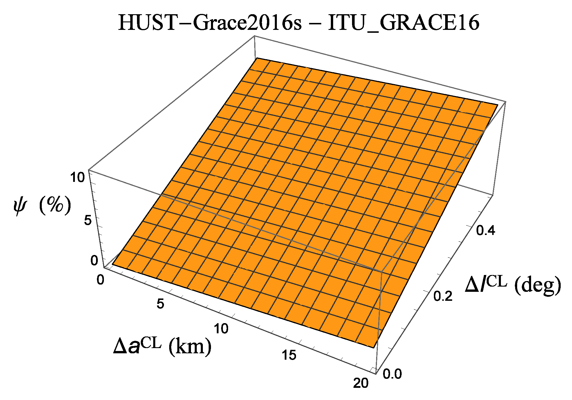
In

Table A2. Strictly upper triangular matrix: absolute values $\Delta {\overline{C}}_{2,0}=\left|{\overline{C}}_{2,0}^{\left(i\right)}-{\overline{C}}_{2,0}^{\left(j\right)}\right|$ of the differences between the estimated normalized Stokes coefficients ${\overline{C}}_{2,0}$ of degree $\ell =2$ and order $m=0$ for the recent GRACE/GOCE-based global gravity field solutions (tide system: zero-tide) $i,j=$ Tongji-Grace02s [62], ITU_GRACE16 [45], HUST-Grace2016s [44], XGM2016 [63] retrieved from the section Static Models of the WEB page of the International Center for Global Earth Models (ICGEM) at http://icgem.gfz-potsdam.de/tom_longtime. Strictly lower triangular matrix: maximum values of the percent error $\psi$ computed from Equation (6) by assuming the figures in the strictly upper triangular matrix for the uncertainty in ${\overline{C}}_{2,0}$. The semimajor axis a and the inclination I of CL were allowed to vary within a range of $a^{\mathrm{CL}}=\mathrm{12,270}\pm 20\mathrm{km},I^{\mathrm{CL}}=70.16\pm 0.5\mathrm{deg}$, respectively. Cfr. with Figure A1.

	Tongji-Grace02s	ITU_GRACE16	HUST-Grace2016s	XGM2016
Tongji-Grace02s	−	$1.9\times {10}^{-10}$	$6\times {10}^{-11}$	$1.2\times {10}^{-10}$
ITU_GRACE16	$8\%$	−	2.5 $\times {\mathbf{10}}^{-\mathbf{10}}$	$6\times {10}^{-11}$
HUST-Grace2016s	$2.5\%$	10%	−	$1.8\times {10}^{-10}$
XGM2016	$5\%$	$3\%$	$8\%$	−

and

Table A3. Strictly upper triangular matrix: absolute values $\Delta {\overline{C}}_{2,0}=\left|{\overline{C}}_{2,0}^{\left(i\right)}-{\overline{C}}_{2,0}^{\left(j\right)}\right|$ of the differences between the estimated normalized Stokes coefficients ${\overline{C}}_{2,0}$ of degree $\ell =2$ and order $m=0$ for the recent GOCE-based global gravity field solutions (tide system: tide-free) $i,j=$ NULP-02s [64], GO_CONS_GCF_2_SPW_R5 [65], IGGT_R1 [47], IfE_GOCE05s [48] retrieved from the section Static Models of the WEB page of the International Center for Global Earth Models (ICGEM) at http://icgem.gfz-potsdam.de/tom_longtime. Strictly lower triangular matrix: maximum values of the percent error $\psi$ computed from Equation (6) by assuming the figures in the strictly upper triangular matrix for the uncertainty in ${\overline{C}}_{2,0}$. The semimajor axis a and the inclination I of CL were allowed to vary within a range of $a^{\mathrm{CL}}=\mathrm{12,270}\pm 20\mathrm{km},I^{\mathrm{CL}}=70.16\pm 0.5\mathrm{deg}$, respectively. Cfr. with Figure A2.

	NULP-02s	GO_CONS_GCF_2_SPW_R5	IGGT_R1	IfE_GOCE05s
NULP-02s	−	$9\times {10}^{-11}$	$2.6\times {10}^{-10}$	$1.7\times {10}^{-9}$
GO_CONS_GCF_2_SPW_R5	$4\%$	−	$1.7\times {10}^{-10}$	$1.8\times {10}^{-9}$
IGGT_R1	$12\%$	$7\%$	−	1.9 $\times {\mathbf{10}}^{-\mathbf{9}}$
IfE_GOCE05s	$70\%$	$80\%$	85%	−

, we adopt the differences $\Delta {\overline{C}}_{2,0}$ between the nominal values of the estimated coefficients ${\overline{C}}_{2.0}^{i/j}$ of several pairs of geopotential models $i,j$, not directly relying upon the SLR data of the LAGEOS family itself, for the uncertainty $\delta J_2$ entering Equation (4); (e.g., [40], p. 1713). From Table A2, which compares some models of the zero-tide system built from GRACE data records differing by their temporal extensions and type of measurements, it turns out that the maximum uncertainty in the systematic bias due to the first even zonal can reach the ≃10% level by using the GRACE-based HUST-Grace2016s [44] and ITU_GRACE16 [45] models; cfr. with Figure A1. Interestingly, the formal errors of such solutions are comparable (see [46], p. 91); indeed, it is

$${\sigma }_{{\overline{C}}_{2,0}}^{\mathrm{HUST}-\mathrm{Grace}2016\mathrm{s}}=9.6\times {10}^{-14},{\sigma }_{{\overline{C}}_{2,0}}^{\mathrm{ITU}\_\mathrm{GRACE}16}=1.2\times {10}^{-13},$$

(7)

so that

$$\frac{{\sigma }_{{\overline{C}}_{2,0}}^{\mathrm{ITU}\_\mathrm{GRACE}16}}{{\sigma }_{{\overline{C}}_{2,0}}^{\mathrm{HUST}-\mathrm{Grace}2016\mathrm{s}}}=1.25.$$

(8)

HUST-Grace2016s is a static global gravity field model obtained by using approximately 13 yr (spanning from January 2003 to April 2015) of GRACE-only data [44]. ITU_GRACE16 is a static global gravity field model computed from GRACE Satellite-to-Satellite-Tracking (SST) data of 50 months collected between April 2009 to October 2013 [45]. For the details of the other models used in Table A2 3.

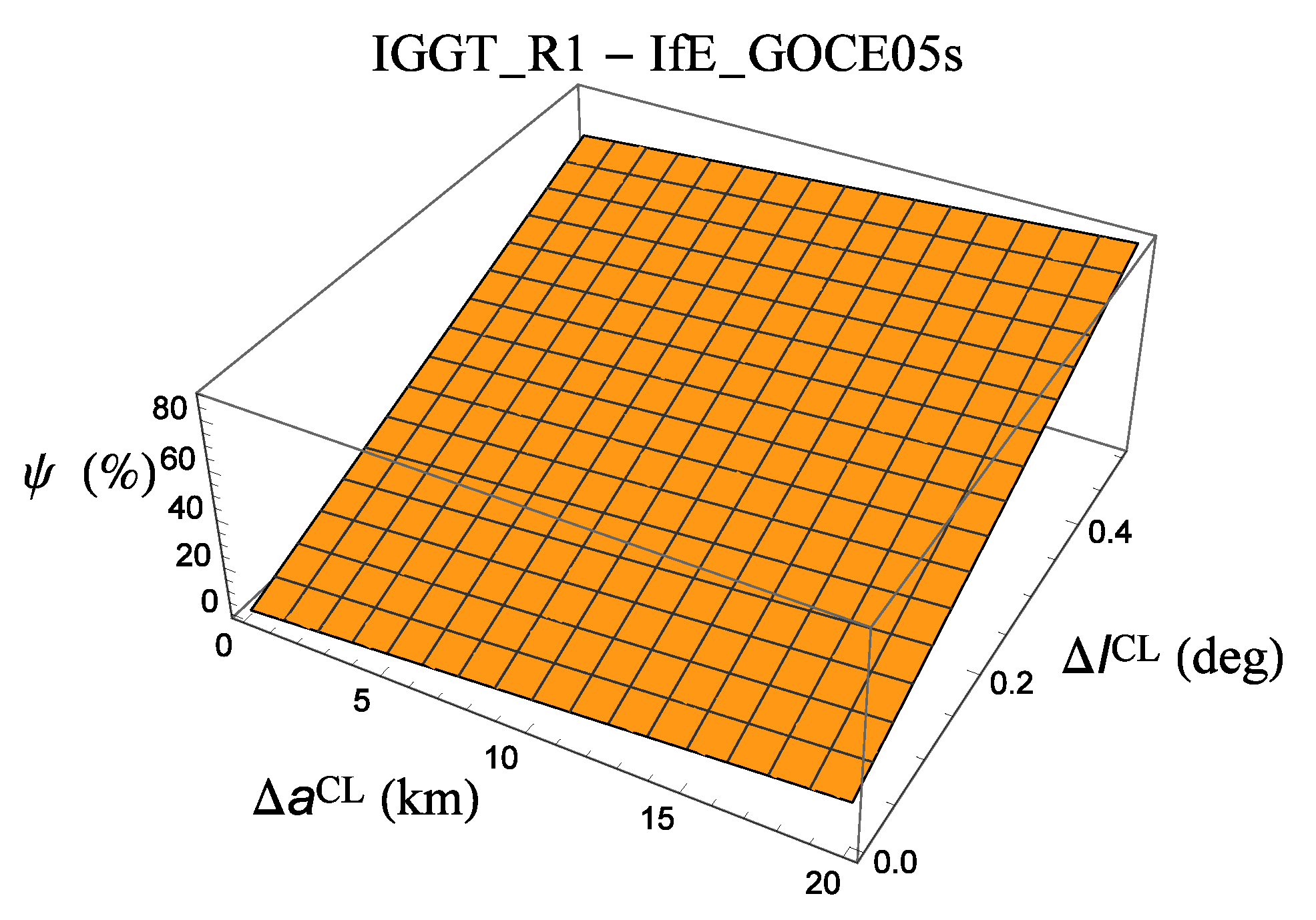
Table A3, showing the impact of some tide-free models from various GOCE data records analyzed with different approaches, tells us that the $J_2$-driven overall uncertainty in the LT test can be as large as ≃85% if the GOCE-based IGGT_R1 [47] and IfE_GOCE05s [48] models are considered; see also Figure A2. Moreover, the (formal) released sigmas of IGGT_R1 and IfE_GOCE05s are comparable since

$${\sigma }_{{\overline{C}}_{2,0}}^{\mathrm{IGGT}\_\mathrm{R}1}=9.7\times {10}^{-11},{\sigma }_{{\overline{C}}_{2,0}}^{\mathrm{IfE}\_\mathrm{GOCE}05\mathrm{s}}=1.8\times {10}^{-11},$$

(9)

so that

$$\frac{{\sigma }_{{\overline{C}}_{2,0}}^{\mathrm{IGGT}\_\mathrm{R}1}}{{\sigma }_{{\overline{C}}_{2,0}}^{\mathrm{IfE}\_\mathrm{GOCE}05\mathrm{s}}}=5.4.$$

(10)

IGGT_R1 [47] relies upon the use of the three invariants of the gravitational gradient tensor (IGGT) to process about 1 yr of GOCE data (2009–2010), while in IfE_GOCE05s [48] almost the same GOCE-only data set is analyzed with either the SST and the Satellite Gravity Gradient (SGG) techniques.4

It is difficult to properly argue about the differences between Table A2 and Table A3 also because, after all, new global gravity field solutions will be available if and when the LT-dedicated L-CL analysis will be performed. Our results should likely be looked just as illustrative of the current state-of-affairs and of the need of not limiting just to one particular model, given the sound possibility that the increasing number of values of $J_2$ will not finally converge to the desired level of accuracy.

A further source of potentially non-negligible systematic uncertainty is as follows. The precessions of Equations (1) and (2), on which Equation (6) is based, hold in a coordinate system whose reference z-axis is aligned with the Earth’s spin axis. Actually, real data reductions are performed with respect to the International Celestial Reference Frame (ICRF) [39] which adopts the mean Earth’s equator at epoch J2000.0 as fundamental reference $\left\{x,y\right\}$ plane. In fact, $\widehat{\mathit{S}}$ does vary in time because of a variety of physical phenomena among which the lunisolar torques inducing the precession of the equinoxes is a major one. Thus, in correctly assessing the systematic bias due to $J_2$, one has to properly account for the fact that, at the time of the data reduction, $\widehat{\mathit{S}}$ will be displaced by a certain amount with respect to the case of Equations (1) and (2), and adequate formulas have to be used. To this aim, the general gravitomagnetic and $J_2$-driven node precessions are [49]

$${\dot{\mathsf{\Omega }}}_{\mathrm{LT}}=\frac{2GScscI}{c^2{a}^3{\left(1-e^2\right)}^{3/2}}\widehat{\mathit{S}}·\widehat{\mathbf{m}},$$

(11)

$${\dot{\mathsf{\Omega }}}_{J_2}=-\frac{3}{2}{n}_{\mathrm{b}}{\left(\frac{R}{a}\right)}^2\frac{cscI{J}_2}{{\left(1-e^2\right)}^2}\left(\widehat{\mathit{S}}·\widehat{\mathbf{m}}\right)\left(\widehat{\mathit{S}}·\widehat{\mathbf{n}}\right).$$

(12)

In Equations (11) and (12), $\widehat{\mathbf{m}}$ is a unit vector in the orbital plane directed transversely to the line of the nodes, while $\widehat{\mathrm{n}}$ is a unit vector perpendiculrar to the orbital plane along the orbital angular momentum. About $\widehat{\mathit{S}}$, its temporal variation, which introduces a time-dependence in the LT and $J_2$ rates of Equations (11) and (12), can be expressed as [50]

$$\begin{array}{cc}\hfill \alpha & \simeq 0.00-0.641{\mathrm{deg}\mathrm{cty}}^{-1}\tau ,\hfill \end{array}$$

(13)

$$\begin{array}{cc}\hfill \delta & \simeq 90\mathrm{deg}-0.557{\mathrm{deg}\mathrm{cty}}^{-1}\tau .\hfill \end{array}$$

(14)

In Equations (13) and (14), $\alpha ,\delta$ are the right ascension (RA) and the declination (DEC) of the Earth’s spin axis, respectively, while $\tau$ is the interval in Julian centuries (of 36525 days) from the standard epoch JD 2451545.0. The Earth’s spin axis can be expressed in terms of $\alpha ,\delta$ as

$$\widehat{\mathit{S}}=\left\{cos\alpha cos\delta ,sin\alpha cos\delta ,sin\delta \right\}.$$

(15)

Thus, if one calculates Equation (6) by means of Equations (11)–(14), a dependence on t and the initial values ${\mathsf{\Omega }}_0^{\mathrm{L}},{\mathsf{\Omega }}_0^{\mathrm{CL}}$ of the nodes of L and CL at the starting epoch of the data reduction which may have a non-negligible impact is introduced. By expanding Equation (15) according to Equations (13) and (14) and neglecting terms quadratic in $\dot{\alpha },\dot{\delta }$, a linear dependence on t occurs. Indeed, one has

$$\widehat{\mathit{S}}\simeq \left\{-\dot{\delta }\tau ,\mathcal{O}\left(\dot{\alpha }\dot{\delta }\right),1+\mathcal{O}\left({\dot{\delta }}^2\right)\right\}.$$

(16)

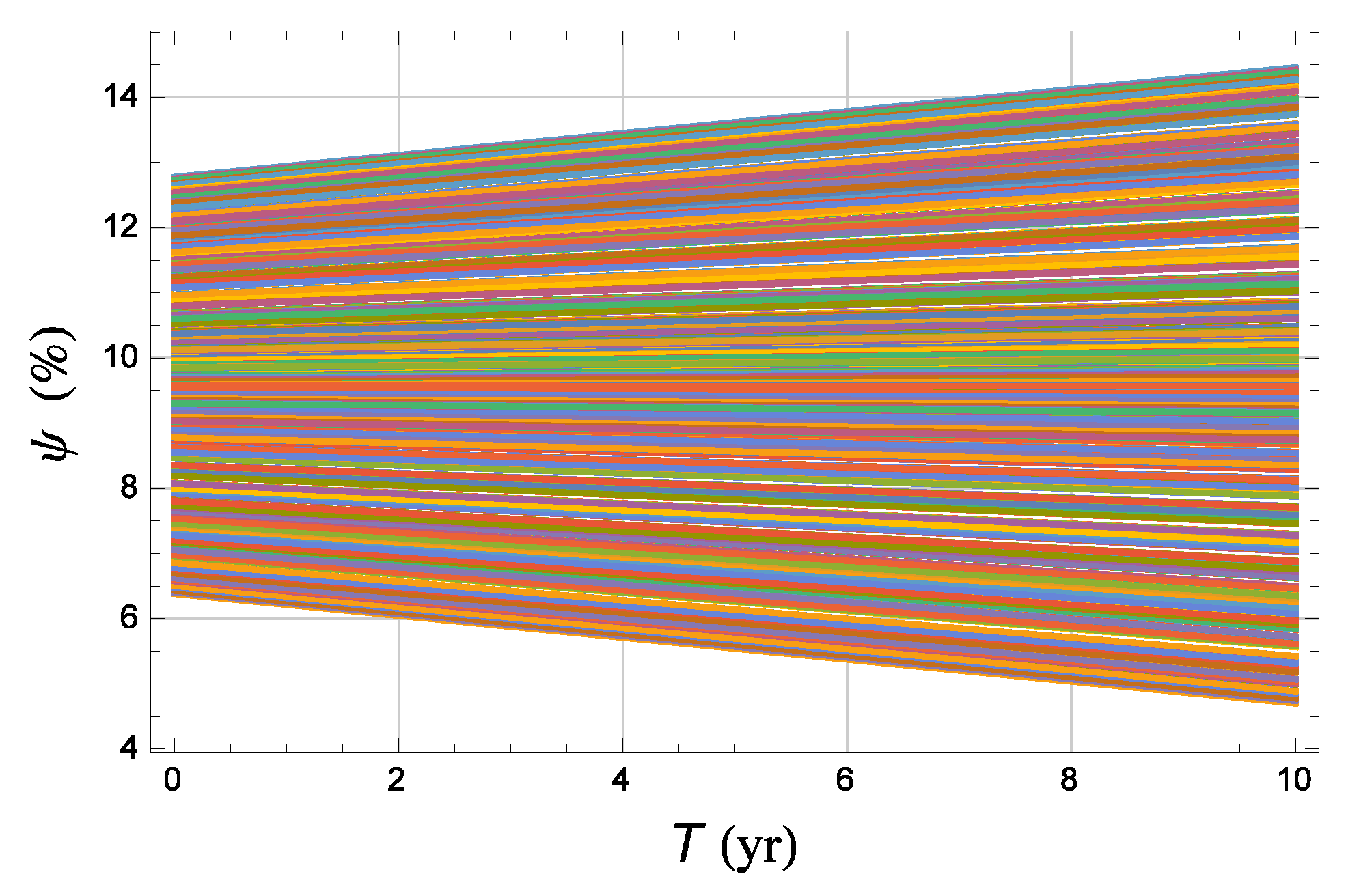
It implies a quadratic signature in the integrated node residuals giving rise to a mild parabolic residual signal. Over temporal intervals just some years long, it would likely superimpose onto the linear LT trend by potentially corrupting its recovery. A similar issue also occurs for other potential sources of systematic errors (see Section 3 and Section 4). Figure A3 depicts the scatter in the values of $\psi$ over $10\mathrm{yr}$ for $\delta {\overline{C}}_{2,0}=2.5\times {10}^{-10}$ (see Table A2) and $\Delta a^{\mathrm{CL}}=20\mathrm{km},\Delta I^{\mathrm{CL}}=0.5\mathrm{deg}$ by allowing ${\mathsf{\Omega }}_0^{\mathrm{L}},{\mathsf{\Omega }}_0^{\mathrm{CL}}$ to vary independently of each other within a $360\mathrm{deg}$ range. It can be noted that $\psi$ finally vary from $5\%$ to about $15\%$.

3. The Indirect Impact of the Earth’s Oblateness through the Secular Decay of the Satellites’ Semimajor Axes

It has been known for several decades that the semimajor axis a of the existing LAGEOS-type satellites experiences a secular decay $\dot{a}<0$ as large as [35,51,52,53]

$$\left|\dot{a}\right|\simeq 0.2-0.9{\mathrm{m}\mathrm{yr}}^{-1}$$

(17)

experimentally determined with an accuracy of the order of [51,52,53]

$${\sigma }_{\dot{a}}\simeq 0.03-0.1{\mathrm{m}\mathrm{yr}}^{-1}.$$

(18)

See Table 2 of Iorio [54]. About LAGEOS, it should be remarked that the experimental accuracy in determining its orbital decay rate has not significantly improved over the past few decades. Indeed, Rubincam [52] reported ${\sigma }_{{\dot{a}}^{\mathrm{L}}}=0.1{\mathrm{mm}\mathrm{d}}^{-1}=0.036{\mathrm{m}\mathrm{yr}}^{-1}$, while ${\sigma }_{{\dot{a}}^{\mathrm{L}}}=0.035{\mathrm{m}\mathrm{yr}}^{-1}$ is quoted in Sośnica et al. [51], Sośnica [53]. Note that the quoted ${\sigma }_{\dot{a}}$ are not due to a priori uncertainties in the acceleration models used; instead, they are a posteriori errors generated in the data reduction procedure.

Neither the pN gravitomagnetic field of the Earth nor its Newtonian oblateness $J_2$ directly affect the semimajor axis a with secular perturbations. Nonetheless, as shown by Iorio [54], the secular decay $\dot{a}<0$ of such an orbital element has a long-term indirect effect on the node $\mathsf{\Omega }$ through its interplay with its classical precession ${\dot{\mathsf{\Omega }}}_{J_2}$ driven by $J_2$. The resulting change over a time span T is [54]

$$\Delta {\mathsf{\Omega }}_{J_2}^{\dot{a}}\simeq \frac{21}{8}{\left(\frac{R}{a_0}\right)}^2\frac{J_{2}cosI}{{\left(1-e^2\right)}^2}\left(\frac{n_{\mathrm{b}}\dot{a}{T}^2}{a_0}\right)+\mathcal{O}\left({\dot{a}}^2{T}^3\right).$$

(19)

In Equation (19), $a_0$ is the semimajor axis at some reference epoch assumed as initial value at the beginning of the observational time span T. To the first order in $\dot{a}$, Equation (19) can be written as

$$\Delta {\mathsf{\Omega }}_{J_2}^{\dot{a}}=K_{J_2}\dot{a},$$

(20)

where

$$K_{J_2}\doteq \frac{\partial \Delta {\mathsf{\Omega }}_{J_2}^{\dot{a}}}{\partial \dot{a}}=\frac{21}{8}{\left(\frac{R}{a_0}\right)}^2\frac{J_{2}cosI}{{\left(1-e^2\right)}^2}\left(\frac{n_{\mathrm{b}}{T}^2}{a_0}\right).$$

(21)

It is quite plausible and reasonable to assume that CL will also finally experience such a subtle orbital decay, although much will likely depend on the actual manufacturing of CL and its surface properties. Thus, it is important to calculate its impact on the proposed use of the sum of the nodes of LAGEOS and CL. It is worthwhile remarking that we will exclusively rely upon the so-far phenomenologically determined values of the secular decays of the semimajor axes of the satellites of the LAGEOS family from real data reductions of long observational records. Stated differently, we will not try to model such an observed orbital feature in terms of some exotic or mundane physical phenomena; for several attempts towards this goal in terms of standard non-gravitational effects, see, e.g., Lucchesi et al. [5], Pardini et al. [35], Rubincam [52,55,56], Scharroo et al. [57]. Since each satellite experiences its own semimajor axis secular rate, $\dot{a}$ must be treated as an independent variable for both satellites in calculating the associated error in the sum of their node shifts, which, thus, reads

$$\delta \left(\Delta {\mathsf{\Omega }}_{\dot{a}}^{\mathrm{tot}}\right)\le \left|K_{J_2}^{\mathrm{L}}\right|{\sigma }_{{\dot{a}}^{\mathrm{L}}}+\left|K_{J_2}^{\mathrm{CL}}\right|{\sigma }_{{\dot{a}}^{\mathrm{CL}}}.$$

(22)

Note that it was assumed that the errors ${\sigma }_{{\dot{a}}^{\mathrm{L}}},{\sigma }_{{\dot{a}}^{\mathrm{CL}}}$ stay constant during the data analysis. Should they change, things would be even more complicated. In this case, contrary to the bias due to the Earth’s even zonal $J_2$, the peculiar orbital configuration of CL does not provide benefits in calculating the systematic error due to ${\sigma }_{\dot{a}}$. Indeed, if $\dot{a}$ were, say, an external parameter common to both satellites as it occurs for $J_2$, the coefficient proportional to ${\sigma }_{\dot{a}}$ would be $\left|K_{J_2}^{\mathrm{L}}+K_{J_2}^{\mathrm{CL}}\right|$. As a result, the corresponding percent error

$$\xi \doteq \frac{\delta \left(\Delta {\mathsf{\Omega }}_{\dot{a}}^{\mathrm{tot}}\right)}{\Delta {\mathsf{\Omega }}_{\mathrm{LT}}^{\mathrm{tot}}}$$

(23)

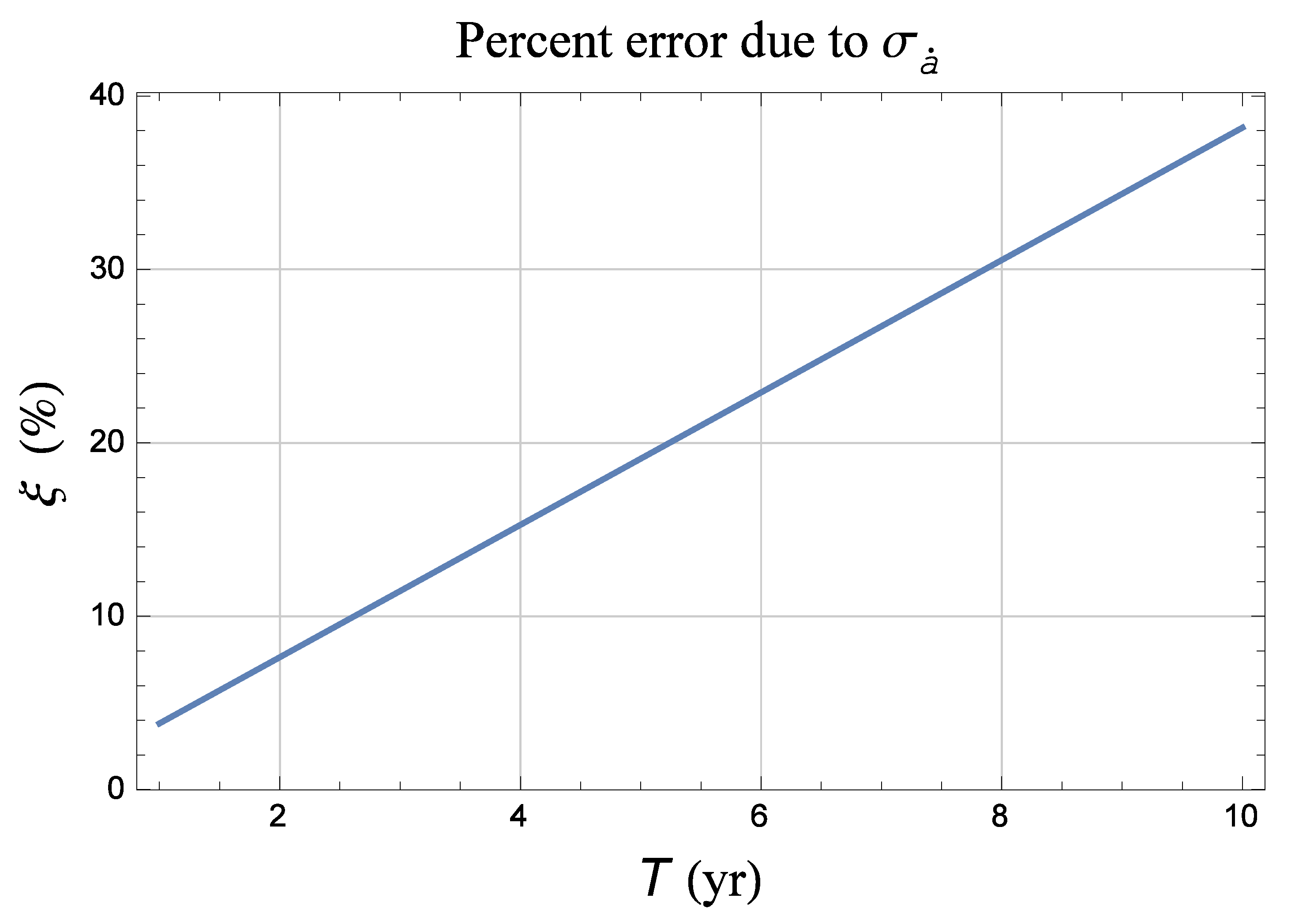
in the total Lense–Thirring node shift, for given values of $\Delta a^{\mathrm{CL}},\Delta I^{\mathrm{CL}}$ and ${\sigma }_{{\dot{a}}^{\mathrm{L}}},{\sigma }_{{\dot{a}}^{\mathrm{CL}}}$, is linear in T. Figure A4 depicts it over a time shift 10 yr long for $\Delta a^{\mathrm{CL}}=10\mathrm{km},\Delta I^{\mathrm{CL}}=0.15\mathrm{deg},{\sigma }_{{\dot{a}}^{\mathrm{L}}}=0.035{\mathrm{m}\mathrm{yr}}^{-1}$. For CL, we hypothesize an improvement of, say, a factor of 3 in the determination of its possible orbital rate decay with respect to LAGEOS by assuming ${\sigma }_{{\dot{a}}^{\mathrm{CL}}}=0.01{\mathrm{m}\mathrm{yr}}^{-1}$. It can be noted that $\xi$ is as large as $20\%$ after 5 yr, reaching $40\%$ after 10 yr. It turns out that, even if it were ${\sigma }_{{\dot{a}}^{\mathrm{CL}}}=0$, the situation would not change too much, with a maximum bias of roughly $\simeq 35\%$ after 10 yr. A breakthrough in the accuracy of the determination of the orbital decay rate of LAGEOS by a factor of 10 would be needed to bring such source of systematic uncertainty down to the percent level; in view of what happened so far in the last decades, it does not seem plausible to occur in the foreseeable future. At least as far as the existing LAGEOS is concerned, the experimental error ${\sigma }_{{\dot{a}}^{\mathrm{L}}}$ has shown so far a very weak time dependence, staying essentially constant over the decades.

For the sake of completeness, we also note that the impact of the uncertainty in $J_2$ in the sum of the corresponding node shifts due to $\dot{a}$ of Equation (19) is negligible with respect to the added Lense–Thirring node rates.

Finally, it is worth noting that the effect considered in this section would act as some sort of parabolic signature in the integrated node residuals, being quadratic in time. Nonetheless, it would be premature and unjustified to argue that its mismodelled component would necessarily decouple from the LT linear signal. Indeed, the resulting parabola would be rather flat, especially over not too long temporal intervals T. Thus, it is likely that the recovery of the gravitomagnetic slope would be impacted by the aforementionded mismodeled competing quadratic effect. A quantitative assessment of the level of such a potential bias is beyond the scope of the present paper since it would require ad hoc data simulations and reductions.

4. The Indirect Impact of the Earth’s Oblateness through the Secular Decay of the Satellites’ Inclination

Despite it seeming that, at present, no experimental determinations of a possible secular decay $\dot{I}$ of the inclination of the LAGEOS-type satellites are publicly available in the literature, there are several standard physical mechanisms of non-gravitational origin, which, in principle, are able to induce such an effect. Thus, despite the content of the present section possibly being deemed as still hypothetical, we will prefer to accurately consider also its possible indirect impact on the classical node precessions driven by the Earth’s oblateness as done for the semimajor axis decay in Section 3.

By inserting

$$I\left(t\right)\simeq I_0+\dot{I}t,$$

(24)

in Equation (2), the total node shift including also the part due to the secular decay of the inclination, integrated over a time span T, is

$$\Delta {\mathsf{\Omega }}_{J_2}={\int }_0^T{\dot{\mathsf{\Omega }}}_{J_2}\left(t\right)dt=\frac{3n_{\mathrm{b}}{R}^2{J}_2\left[sin{I}_0-sin\left(I_0+\dot{I}T\right)\right]}{2a^2{\left(1-e^2\right)}^2\dot{I}}.$$

(25)

In Equations (24) and (25), $I_0$ is the inclination at some reference epoch assumed as initial value at the beginning of the observational time span T. Note that, in the limit $\dot{I}\to 0$, Equation (25) reduces just to Equation (2). By posing

$$\theta \doteq \dot{I}T\ll 1,$$

(26)

as is the case for the LAGEOS-type satellites over even multidecadal time spans T (see Equations (47) and (49) below), let us expand the trigonometric functions $sin\alpha ,cos\alpha$ in $sin\left(I_0+\alpha \right)$ entering Equation (25) as

$$\begin{array}{cc}\hfill cos\theta & \simeq 1-\frac{{\theta }^2}{2},\hfill \end{array}$$

(27)

$$\begin{array}{cc}\hfill sin\theta & \simeq \theta -\frac{{\theta }^3}{6}.\hfill \end{array}$$

(28)

Thus, from Equation (25), one can approximately obtain for the $\dot{I}$-induced node shift

$$\Delta {\mathsf{\Omega }}_{J_2}^{\dot{I}}\simeq \frac{n_{\mathrm{b}}{J}_2{R}^2\dot{I}{T}^2\left(\dot{I}Tcos{I}_0+3sin{I}_0\right)}{4a^2{\left(1-e^2\right)}^2}.$$

(29)

From Equation (29), it turns out that

$$\delta \left(\Delta {\mathsf{\Omega }}_{J_2}^{\dot{I}}\right)\le \left|\frac{\partial \Delta {\mathsf{\Omega }}_{J_2}^{\dot{I}}}{\partial \dot{I}}\right|{\sigma }_{\dot{I}}\simeq \left|\frac{n_{\mathrm{b}}{J}_2{R}^2{T}^2\left(2\dot{I}Tcos{I}_0+3sin{I}_0\right)}{4a^2{\left(1-e^2\right)}^2}\right|{\sigma }_{\dot{I}}.$$

(30)

By posing

$${\mathcal{I}}_{J_2}\doteq \frac{n_{\mathrm{b}}{J}_2{R}^2{T}^2\left(2\dot{I}Tcos{I}_0+3sin{I}_0\right)}{4a^2{\left(1-e^2\right)}^2},$$

(31)

the total systematic bias in the sum of the nodes is, thus,

$$\delta \left(\Delta {\mathsf{\Omega }}_{\dot{I}}^{\mathrm{tot}}\right)\le \left|{\mathcal{I}}_{J_2}^{\mathrm{L}}\right|{\sigma }_{{\dot{I}}^{\mathrm{L}}}+\left|{\mathcal{I}}_{J_2}^{\mathrm{CL}}\right|{\sigma }_{{\dot{I}}^{\mathrm{CL}}}.$$

(32)

Not only the experimental accuracy ${\sigma }_{\dot{I}}$ in measuring a possible decay of the orbital plane, but also its nominal value $\dot{I}$ enter Equation (32) through Equation (31). Thus, at least in principle, it is important to try to give a plausible order of magnitude of such a subtle phenomenon. Below, we will consider only the effect of the neutral and charged drag, whose disturbing acceleration can be modeled as [19,58]

$${\mathit{A}}_{\mathrm{drag}}=-\frac{1}{2}{C}_{\mathrm{D}}\mathsf{\Sigma }\rho V\mathit{V}.$$

(33)

In Equation (33), $C_{\mathrm{D}},\mathsf{\Sigma },\rho ,\mathit{V}$ are the satellite’s drag coefficient and area-to-mass ratio, the atmospheric density at the satellite’s height, and the satellite’s velocity with respect to the Earth’s atmosphere, respectively. It can be shown that, among other things, Equation (33) also induces a secular variation of the inclination I given by [19,59]

$$\frac{\mathrm{d}I}{\mathrm{d}t}=-\frac{1}{4}{C}_{\mathrm{D}}\mathsf{\Sigma }\rho {\omega }_{\mathrm{atm}}asinI.$$

(34)

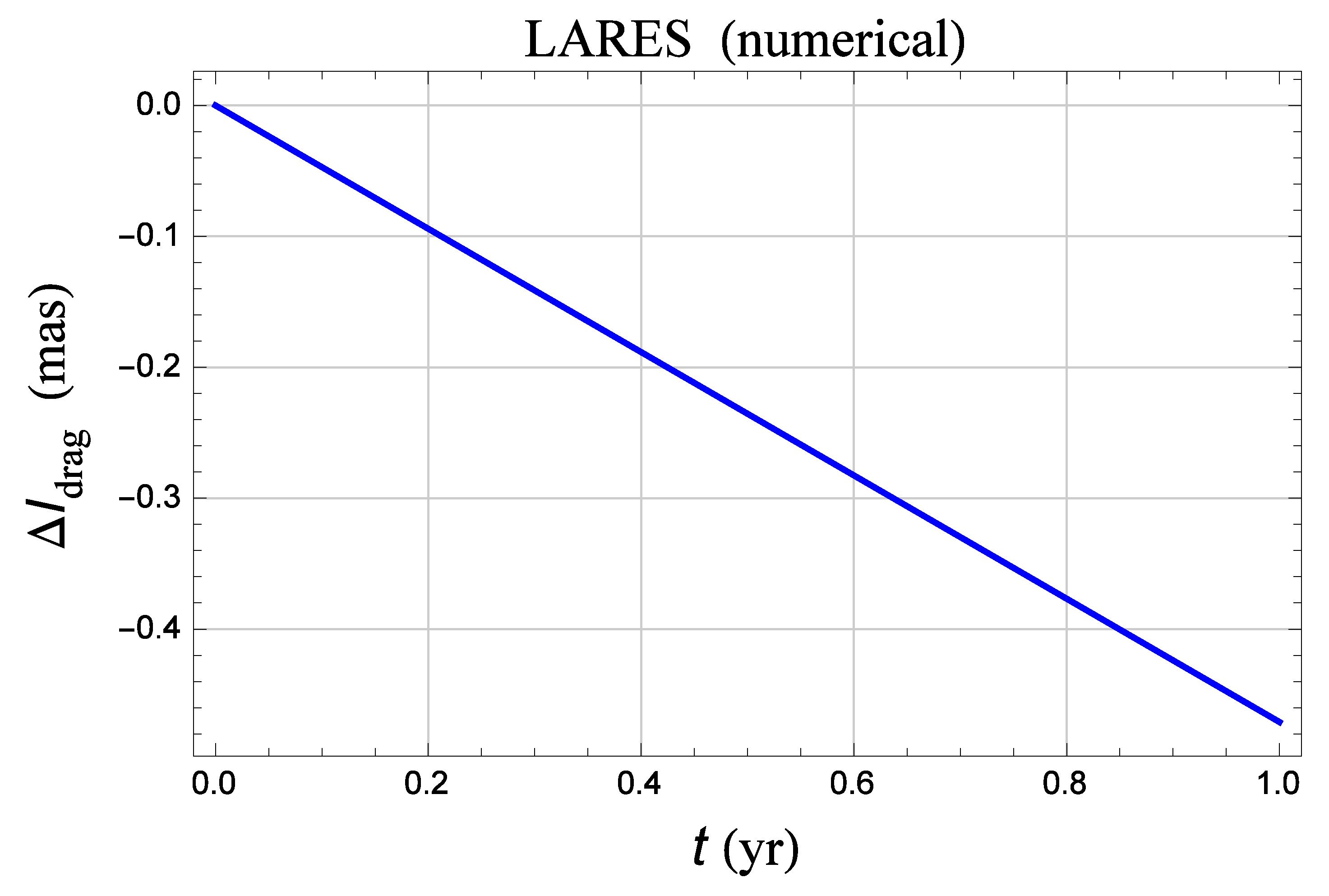
In Equation (34), ${\omega }_{\mathrm{atm}}$ is the angular velocity of Earth’s atmosphere. We will, first, confirm the validity of Equation (34) in the case of LARES by comparing its predicted theoretical rate with a numerical integration of its equations of motion. For such a satellite, it is [35]

$$\begin{array}{cc}\hfill C_{\mathrm{D}}& =3.5,\hfill \end{array}$$

(35)

$$\begin{array}{cc}\hfill \mathsf{\Sigma }& =2.69\times {10}^{-4}{\mathrm{m}}^2{\mathrm{kg}}^{-1},\hfill \end{array}$$

(36)

$$\begin{array}{cc}\hfill {\rho }_{\mathrm{neutral}}& =5.9\times {10}^{-16}\mathrm{kg}{\mathrm{m}}^{-3},\hfill \end{array}$$

(37)

$$\begin{array}{cc}\hfill {\omega }_{\mathrm{atm}}& \simeq {\omega }_{\oplus }=7.29\times {10}^{-5}{\mathrm{s}}^{-1},\hfill \end{array}$$

(38)

so that Equation (34) allows for predicting a nominal decay of the order of [59]

$${\dot{I}}_{\mathrm{drag}}^{\mathrm{LR}}=-0.5\mathrm{mas}{\mathrm{yr}}^{-1}.$$

(39)

In Equation (38), ${\omega }_{\oplus }$ is the angular velocity of Earth. The analytical result of Equation (39) is supported by a numerical integration of the equations of motion of LARES in rectangular Cartesian coordinates with and without Equation (33). Figure A5 displays the resulting time series for the drag-induced inclination shift $\Delta I_{\mathrm{drag}}\left(t\right)$ of LARES over a time span 1 yr long; a negative trend with just the same size of Equation (39) is clearly apparent. It can be shown that our approach is also able to reproduce, both analytically and numerically, the observed secular decay of the semimajor axis of LARES, in agreement with the finding by Pardini et al. [35] who found that the neutral atmospheric drag is able to explain almost entirely such a phenomenon. Thus, confident of our strategy, we can, now, safely apply it to LAGEOS and CL. At the altitude of 5900 km, the total neutral atmospheric density experienced by LAGEOS is of the order of

$${\rho }_{\mathrm{neutral}}^{\mathrm{L}}\simeq 8.4\times {10}^{-18}\mathrm{kg}{\mathrm{m}}^{-3}$$

(40)

due to neutral hydrogen H, corresponding to a hydrogen number density of $5\times {10}^9{\mathrm{m}}^{-3}$ [60]. As far as the charged particles in the plasmasphere are concerned,

$${\rho }_{{\mathrm{H}}^{+}}^{\mathrm{L}}\simeq 5.0\times {10}^{-18}\mathrm{kg}{\mathrm{m}}^{-3}$$

(41)

comes from protons H${}^{+}$ for a proton number density of $3\times {10}^9{\mathrm{m}}^{-3}$ [60],

$${\rho }_{{\mathrm{He}}^{+}}^{\mathrm{L}}\simeq 7.2\times {10}^{-18}\mathrm{kg}{\mathrm{m}}^{-3}$$

(42)

refers to Helium ions He${}^{+}$, while

$${\rho }_{{\mathrm{O}}^{+}}^{\mathrm{L}}\simeq 4.6\times {10}^{-17}\mathrm{kg}{\mathrm{m}}^{-3}$$

(43)

is attributable to Oxygen ions O${}^{+}$. However, as noted in Rubincam [60], Equations (41) and (43) have to be divided by a factor of 2 since LAGEOS spends just half its time in the plasmasphere. Thus, the total charged density actually felt by LAGEOS is about

$${\rho }_{\mathrm{ch}}^{\mathrm{L}}\simeq 2.9\times {10}^{-17}\mathrm{kg}{\mathrm{m}}^{-3}.$$

(44)

In calculating the acceleration due to charged drag with Equation (33), the charged drag coefficient of LAGEOS can be as large as [19]

$$C_{\mathrm{D}}^{\mathrm{ch}}\simeq 20,$$

(45)

while its area-to-mass ratio amounts to

$$\mathsf{\Sigma }=7\times {10}^{-4}{\mathrm{m}}^2{\mathrm{kg}}^{-1}.$$

(46)

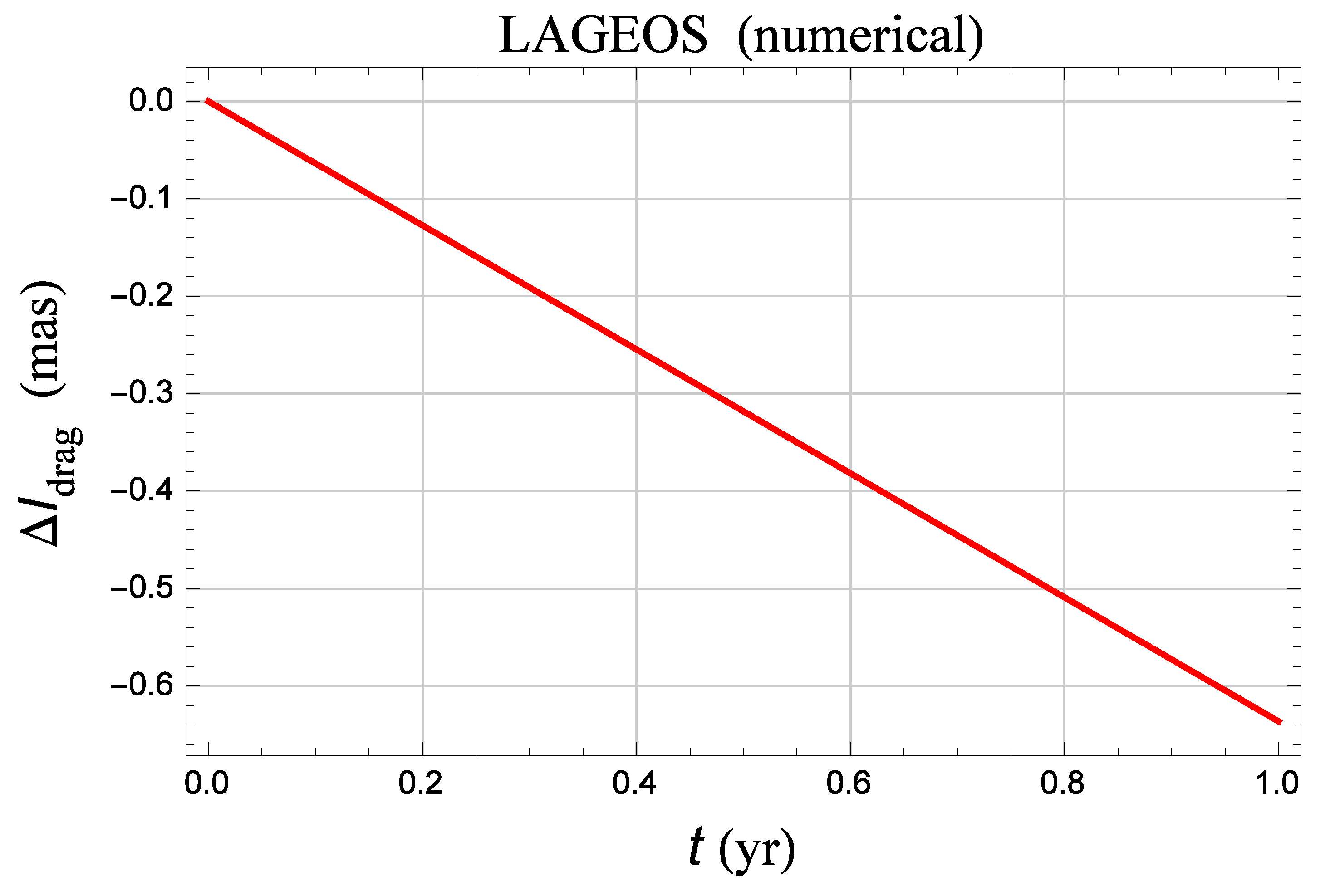
Thus, both Equation (34) and a numerical integration of the equations of motion, whose outcome is displayed in Figure A6, return a secular decay of the orbital plane of LAGEOS due to neutral and charged atmospheric drag of the order of

$${\dot{I}}_{\mathrm{drag}}^{\mathrm{L}}\simeq -0.7\mathrm{mas}{\mathrm{yr}}^{-1}.$$

(47)

In the case of CL, since from the satellite’s physical parameteres released by Ciufolini et al. [38] it can be inferred

$$\mathsf{\Sigma }=4\times {10}^{-4}{\mathrm{m}}^2{\mathrm{kg}}^{-1},$$

(48)

the drag-induced inclination decay would amount to

$${\dot{I}}_{\mathrm{drag}}^{\mathrm{CL}}\simeq -0.4\mathrm{mas}{\mathrm{yr}}^{-1}$$

(49)

by assuming the same value of Equation (45) for its $C_{\mathrm{D}}^{\mathrm{ch}}$. Incidentally, Equations (47) and (49) confirm the validity of the assumption made in Equation (26). In addition, thermal effects connected with the orientation and magnitude of the satellite’s spin axis [55] can induce a secular decay on I [29]; thus, the actual overall size of such a phenomenon may be larger than Equations (47) and (49).

For some reasons, only $\dot{a}$ has been experimentally investigated so far by satellite geodesists; it is expected that, sooner or later, they will look also at the inclination by releasing a best estimate for the predicted inclination decay $\dot{I}$ along with its associated error ${\sigma }_{\dot{I}}$. For the sake of convenience, we may tentatively assume

$${\sigma }_{\dot{I}}\simeq \left(5-10\%\right)\dot{I}=0.035-0.07\mathrm{mas}{\mathrm{yr}}^{-1}.$$

(50)

It is the same percent error of the actually measured $\dot{a}$. The present assumption that the expected secular decay of the inclination will be measured with the same fractional accuracy as the decay of the semimajor axis should be regarded just as a, hopefully, plausible guess in view of the lingering lacking of actual experimental determinations of it. Note that Ciufolini et al. [46] claim to be able to determine the inclination of LAGEOS within an accuracy of just $30\mathsf{\mu }\mathrm{as}=0.03\mathrm{mas}$. About the overall temporal pattern of the bias due to such a potential source of systematic error, the same considerations as in Section 2 and Section 3 about the temporal variation of the Earth’s spin axis and the cross correlation between $J_2$ and $\dot{a}$ hold. Figure A7 depicts

$$\chi \doteq \frac{\delta \left(\Delta {\mathsf{\Omega }}_{\dot{I}}^{\mathrm{tot}}\right)}{\Delta {\mathsf{\Omega }}_{\mathrm{LT}}^{\mathrm{tot}}}$$

(51)

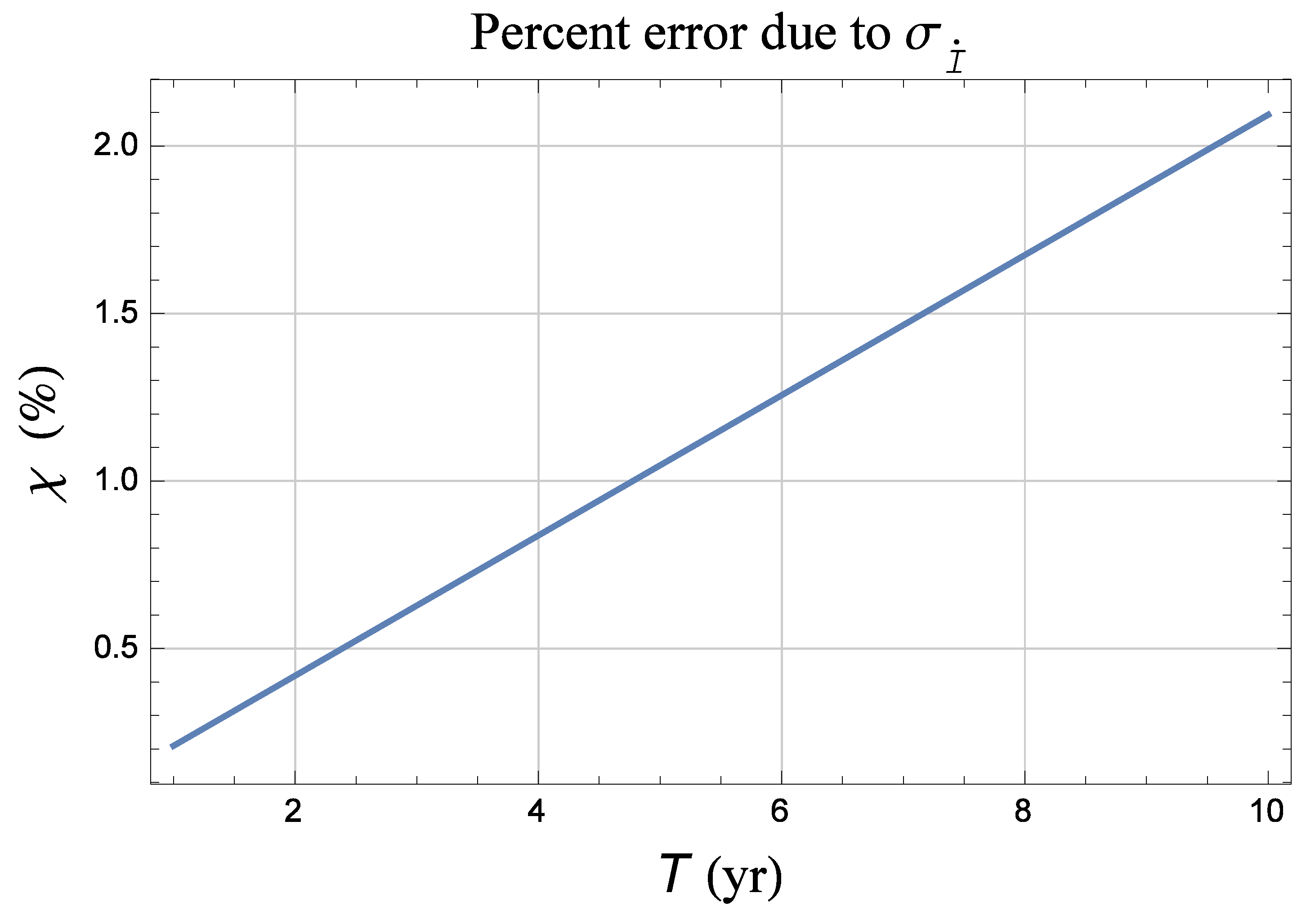
for given values of $\Delta a^{\mathrm{CL}},\Delta I^{\mathrm{CL}},{\dot{I}}^{\mathrm{L}},{\dot{I}}^{\mathrm{CL}},{\sigma }_{{\dot{I}}^{\mathrm{L}}},and{\sigma }_{{\dot{I}}^{\mathrm{CL}}}$ over a time shift 10 yr long. For the orbital shifts of CL, we assumed $\Delta a^{\mathrm{CL}}=10\mathrm{km},\Delta I^{\mathrm{CL}}=0.15\mathrm{deg}$. As far as the inclination decays and their putative errors, we took ${\sigma }_{{\dot{I}}^{\mathrm{L}/\mathrm{CL}}}=0.03{\mathrm{mas}\mathrm{yr}}^{-1}$ along with Equations (47) and (49). It turns out that the nominal value $\dot{I}$ of the expected inclination decay does not has a relevant impact on the total bias $\chi$; even rescaling $\dot{I}$ by a factor of 10 for both satellites does not alter it. Thus, accurately predicting all the possible contributions to $\dot{I}$ does not appear, actually, so important in the present context. On the contrary, ${\sigma }_{\dot{I}}$ is of crucial importance. Indeed, while for their previously listed values the total bias can reach $2\%$ of the summed LT shifts, as shown by Figure A7, by increasing them up to, say, ${\sigma }_{\dot{I}}=0.2{\mathrm{mas}\mathrm{yr}}^{-1}$ would push $\chi$ up to to $14\%$.

5. Conclusions

According to Ciufolini and coworkers, the sum of the precessions of the nodes of the existing LAGEOS satellite and the future CiufoLares (also known-in a more anodyne fashion-as LARES 2), to be launched in 2019 with a VEGA C rocket, should provide us with a ≃0.2% test of frame-dragging in the field of the Earth whose imperfectly known even zonal harmonics should contribute just $0.1\%$ of the total error budget. Actually, it seems difficult for such an ambitious goal to be reached because of the direct and indirect impact of the competing classical node precessions mainly induced by the first even zonal of the geopotential.

On the one hand, according to some of the latest GRACE/GOCE-based global gravity field solutions released by various international institutions in 2016–2017, the lingering scatter of their determinations of such a fundamental geophysical parameter would directly affect the sum of the nodes with an uncancelled mismodelled total precession, which, in some cases, may reach even several dozen percentage points of the total Lense–Thirring effect for departures of the orbital elements of CiufoLares as little as $20\mathrm{km}$ and $0.5\mathrm{deg}$. Other more favorable scenarios point towards uncertainties of the order of ≃3–10%. A further source of systematic uncertainty is given by the dependence on the initial values of the satellites’ nodes introduced by the unavoidable displacement of the Earth’s spin axis with respect to its direction at the reference epoch J2000.0 when the data reduction will be finally performed in the next years by using the ICRF. The insertion of the new SLR target in an orbit as close as possible to the ideal butterfly configuration with LAGEOS will be crucial for effectively controlling such an insidious source of systematic error in view of the persisting difficulties in effectively constraining, at least to the desired level of accuracy for a successful test of the Lense–Thirring effect, the first even zonal of the geopotential.

On the other hand, the classical node precession due to the oblateness of the Earth exerts a further, even subtler, but not less potentially insidious, aliasing effect on the relativistic signature of interest in an indirect way through its coupling with the secular decay which has been phenomenologically measured so far for the semimajor axis of all the existing members of the LAGEOS family. Indeed, it turned out that the associated bias on the sum of the nodes is unaffected by the peculiar orbital geometry of CiufoLares, being impacted crucially by the accuracy in determining the satellites’ orbital decay. Unfortunately, in the case of LAGEOS, after more than 30 yr, no substantial improvements have occurred so far in improving our knowledge of the rate of decreasing of its semimajor axis. Even by assuming that the forthcoming satellite will experience a more accurately known analogous effect, the resulting systematic uncertainty may reach ≃20–40% of the Lense–Thirring signal after 5–10 yr. An analogous indirect bias should occur due to the expected secular decay of the inclination of the orbital planes, although no experimental records for such an effect on the LAGEOS-type spacecraft are yet available in the literature. Thus, such a potential further source of systematic error should be currently deemed as hypothetical, although plausible and well rooted in established standard non-gravitational physics. Depending on its actual experimental accuracy, its impact on the combined Lense–Thirring signature may be in the range ≃2–14% after 10 yr. We note that the indirect effects of the Earth’s rotation pole position, and the secular decays of the semimajor axis and the inclination would affect the time series of the integrated node residuals with a quadratic temporal signature. This does not necessarily mean that it would neatly decouple from the linear Lense–Thirring effect since the residual parabolic curve would be likely rather smooth and poorly distinguishable from a secular trend, especially over relatively short observational time spans. In order to quantitatively assess how much the recovery of the gravitomagnetic slope would be impacted by the aforementionded mismodeled competing quadratic effects, a full simulation of the time series of the sum of the nodes along with a best fit with a parabolic curve would be required; it is beyond the scope of the present preliminary analysis.

In conclusions, the desired goal of a ≃0.1% test of the gravitomagnetic orbital precessions with LAGEOS and CiufoLares seems, at least at present, rather unlikely to be met. In addition to a very strict adherence of the actual orbit of the new spacecraft to its ideal one, a breakthrough of one order of magnitude in determining both the terrestrial first even zonal harmonic and the secular decrease of the semimajor axis of LAGEOS (and from the perspective of CiufoLares as well) would be required to yield a test of some percent by using the sum of the nodes.

References

- Combrinck, L. Sciences of Geodesy I; Xu, G., Ed.; Springer: Berlin/Heidelberg, Germany, 2010; pp. 301–338. [Google Scholar]
- Ciufolini, I.; Sindoni, G.; Paolozzi, A.; Paris, C. The Contribution of LARES to Global Climate Change Studies With Geodetic Satellites. In Proceedings of the 2015 IEEE Aerospace Conference, Big Sky, MT, USA, 7–14 March 2015; pp. 1–8. [Google Scholar]
- Combrinck, L.S. Testing the general relativity theory through the estimation of ppn parameters? And & zlig; using satellite laser ranging data. South African Journal of Geology. S. Afr. J. Geol. 2011, 114, 549–560. [Google Scholar]
- Combrinck, L.S. Sciences of Geodesy II; Xu, G., Ed.; Springer: Berlin/Heidelberg, Germany, 2013; pp. 53–95. [Google Scholar]
- Lucchesi, D.M.; Anselmo, L.; Bassan, M.; Pardini, C.; Peron, R.; Pucacco, G.; Visco, M. Testing the gravitational interaction in the field of the Earth via satellite laser ranging and the Laser Ranged Satellites Experiment (LARASE). Class. Quant. Grav. 2015, 32, 155012. [Google Scholar] [CrossRef]
- Peron, R. Testing General Relativistic Predictions with the LAGEOS Satellites. Adv. High Energy Phys. 2014, 2014, 791367. [Google Scholar] [CrossRef]
- Pfister, H. On the history of the so-called Lense-Thirring effect. Gener. Relat. Gravit. 2007, 39, 1735–1748. [Google Scholar] [CrossRef] [Green Version]
- Pfister, H. The Eleventh Marcel Grossmann Meeting on Recent Developments in Theoretical and Experimental General Relativity, Gravitation and Relativistic Field Theories; Kleinert, H., Jantzen, R.T., Ruffini, R., Eds.; World Scientific: Singapore, 2008; pp. 2456–2458. [Google Scholar]
- Pfister, H. Relativity and Gravitation. In Springer Proceedings in Physics; Bičák, J., Ledvinka, T., Eds.; Springer: Berlin/Heidelberg, Germany, 2014; Volume 157, pp. 191–197. [Google Scholar]
- Lense, J.; Thirring, H. On the influence of the proper rotation of a central body on the motion of the planets and the moon, according to Einstein’s theory of gravitation. Phys. Z 1918, 19, 156–163. [Google Scholar]
- Thorne, K.S. Near Zero: New Frontiers of Physics; Fairbank, J.D., Deaver, B.S., Jr., Everitt, C.W.F., Michelson, P.F., Eds.; FW Freeman and Company: New York, NY, USA, 1988; pp. 573–586. [Google Scholar]
- Thorne, K.S.; MacDonald, D.A.; Price, R.H. (Eds.) Black Holes: The Membrane Paradigm; Yale University Press: Yale, CT, USA, 1986. [Google Scholar]
- Penrose, R.; Floyd, R.M. Extraction of rotational energy from a black hole. Nat. Phys. Sci. 1971, 229, 177–179. [Google Scholar] [CrossRef]
- Williams, R.K. Gravitomagnetic Field and Penrose Scattering Processes. Ann. N. Y. Acad. Sci. 2005, 1045, 232–245. [Google Scholar] [CrossRef] [PubMed]
- Ciufolini, I.; Paolozzi, A.; Koenig, R.; Pavlis, E.C.; Ries, J.; Matzner, R.; Gurzadyan, V.; Penrose, R.; Sindoni, G.; Paris, C. Fundamental Physics and General Relativity with the LARES and LAGEOS satellites. Nucl. Phys. B Proc. Suppl. 2013, 243–244, 180–193. [Google Scholar] [CrossRef]
- Iorio, L.; Lichtenegger, H.I.M.; Ruggiero, M.L.; Corda, C. Phenomenology of the Lense-Thirring effect in the solar system. Astrophys. Space Sci. 2011, 331, 351–395. [Google Scholar] [CrossRef]
- Renzetti, G. History of the attempts to measure orbital frame-dragging with artificial satellites. Cent. Eur. J. Phys. 2013, 11, 531–544. [Google Scholar] [CrossRef] [Green Version]
- de Moraes, R.V. Non-gravitational disturbing forces. Adv. Space Res. 1994, 14, 45–68. [Google Scholar] [CrossRef]
- Milani, A.; Nobili, A.M.; Farinella, P. Non-Gravitational Perturbations and Satellite Geodesy; Adam Hilger: Bristol, UK, 1987. [Google Scholar]
- Sehnal, L. Satellite Dynamics. COSPAR-IAU-IUTAM (International Union of Theoretical and Applied Mechanics); Giacaglia, G.E.O., Stickland, A.C., Eds.; Springer: Berlin/Heidelberg, Germany, 1975; pp. 304–330. [Google Scholar]
- Kaula, W.M. Theory of Satellite Geodesy; Dover Publications: New York, NY, USA, 2000. [Google Scholar]
- Lambeck, K.; Cazenave, A.; Balmino, G. Solid Earth and ocean tides estimated from satellite orbit analyses. Rev. Geophys. Space Phys. 1974, 12, 421–434. [Google Scholar] [CrossRef]
- Rosborough, G.W. Satellite Orbit Perturbations Due to Geopotential; CSR-86-1; Center for Space Research: Austin, TX, USA, 1986. [Google Scholar]
- Bertotti, B.; Farinella, P.; Vokrouhlický, D. Physics of the Solar System: Dynamics and Evolution, Space Physics, and Spacetime Structure; Kluwer Academic Press: Dordrecht, The Netherlands, 2003. [Google Scholar]
- Kopeikin, S.; Efroimsky, M.; Kaplan, G. Relativistic Celestial Mechanics of the Solar System; Wiley-VCH: Weinheim, Germany, 2011. [Google Scholar]
- Poisson, E.; Will, C.M. Gravity; Cambridge University Press: Cambridge, UK, 2014. [Google Scholar]
- Xu, G.; Xu, J. Orbits: 2nd Order Singularity-Free Solutions; Springer: Berlin, Germany, 2013. [Google Scholar]
- Capderou, M. Handbook of Satellite Orbits: From Kepler to GPS; Springer: Berlin/Heidelberg, Germany, 2014. [Google Scholar]
- Lucchesi, D.M. Reassessment of the error modelling of non-gravitational perturbations on LAGEOS II and their impact in the Lense–Thirring derivation—Part II. Planet. Space Sci. 2002, 50, 1067–1100. [Google Scholar] [CrossRef]
- Pavlis, E.C.; Iorio, L. The impact of tidal errors on the determination of the Lense–Thirring effect from satellite laser ranging. Int. J. Mod. Phys. D 2002, 11, 599–618. [Google Scholar] [CrossRef]
- Van Patten, R.A.; Everitt, C.W.F. A possible experiment with two counter-orbiting drag-free satellites to obtain a new test of einstein’s general theory of relativity and improved measurements in geodes. Celest. Mech. Dyn. Astr. 1976, 13, 429–476. [Google Scholar] [CrossRef]
- Ciufolini, I. Measurement of the Lense-Thirring drag on high-altitude, laser-ranged artificial satellites. Phys. Rev. Lett. 1986, 56, 278–281. [Google Scholar] [CrossRef] [PubMed]
- Lhotka, C.; Celletti, A.; Galeş, C. Poynting? Robertson drag and solar wind in the space debris problem. Mon. Notice R. Astron. Soc. 2016, 460, 802–815. [Google Scholar] [CrossRef]
- Lucchesi, D.M. Reassessment of the error modelling of non-gravitational perturbations on LAGEOS II and their impact in the Lense–Thirring determination. Part I. Planet. Space Sci. 2001, 49, 447–463. [Google Scholar] [CrossRef]
- Pardini, C.; Anselmo, L.; Lucchesi, D.M.; Peron, R. On the secular decay of the LARES semi-major axis. Acta Astronaut. 2017, 140, 469–477. [Google Scholar] [CrossRef]
- Sehnal, L. Effects of the terrestrial infrared radiation pressure on the motion of an artificial satellite. Celest. Mech. Dyn. Astr. 1981, 25, 169–179. [Google Scholar] [CrossRef]
- Ciufolini, I.; Paolozzi, A.; Pavlis, E.C.; Koenig, R.; Ries, J.; Gurzadyan, V.; Matzner, R.; Penrose, R.; Sindoni, G.; Paris, C.; et al. A test of general relativity using the LARES and LAGEOS satellites and a GRACE Earth gravity model. Eur. Phys. J. C 2016, 76, 120. [Google Scholar] [CrossRef] [PubMed]
- Ciufolini, I.; Paolozzi, A.; Pavlis, E.C.; Sindoni, G.; Koenig, R.; Ries, J.C.; Matzner, R.; Gurzadyan, V.; Penrose, R.; Rubincam, D. A new laser-ranged satellite for General Relativity and space geodesy: I. An introduction to the LARES2 space experiment. Eur. Phys. J. Plus 2017, 132, 336. [Google Scholar] [CrossRef]
- IERS Conventions. 2010. Available online: https://www.iers.org/SharedDocs/Publikationen/EN/IERS/Publications/tn/TechnNote36/tn36.pdf?__blob=publicationFile&v=1 (accessed on 16 October 2018).
- Ciufolini, I. On a new method to measure the gravitomagnetic field using two orbiting satellites. Nuovo Cimento A 1996, 109, 1709–1720. [Google Scholar] [CrossRef]
- Ciufolini, I.; Pavlis, E.C.; Sindoni, G.; Ries, J.C.; Paolozzi, A.; Matzner, R.; Koenig, R.; Paris, C. A new laser-ranged satellite for General Relativity and space geodesy: II. Monte Carlo simulations and covariance analyses of the LARES 2 experiment. Eur. Phys. J. Plus 2017, 132, 337. [Google Scholar] [CrossRef]
- Mayer-Gürr, T. The GOCO consortium. In Proceedings of the European Geosciences Union General Assembly 2015, Vienna, Austria, 12–17 April 2015; Volume 1. [Google Scholar]
- Ciufolini, I.; Lucchesi, D.; Vespe, F.; Mandiello, A. Measurement of dragging of inertial frames and gravitomagnetic field using laser-ranged satellites. Nuovo Cimento A 1996, 109, 575–590. [Google Scholar] [CrossRef]
- Zhou, H.; Luo, Z.; Zhou, Z.; Zhong, B.; Hsu, H. HUST-Grace2016s: A new GRACE static gravity field model derived from a modified dynamic approach over a 13-year observation period. Adv. Space Res. 2017, 60, 597–611. [Google Scholar] [CrossRef]
- Akyilmaz, O.; Ustun, A.; Aydin, C.; Arslan, N.; Doganalp, S.; Guney, C.; Mercan, H.; Uygur, S.O.; Uz, M.; Yagci, O. ITU_GRACE16 The Global Gravity Field Model Including GRACE Data up to Degree and Order 180 of ITU and Other Collaborating Institutions. 2016. Available online: http://doi.org/10.5880/icgem.2016.006 (accessed on 16 October 2018).
- Ciufolini, I.; Paolozzi, A.; Pavlis, E.C.; Ries, J.C.; Koenig, R.; Matzner, R.A.; Sindoni, G.; Neumayer, H. Towards a One Percent Measurement of Frame Dragging by Spin with Satellite Laser Ranging to LAGEOS, LAGEOS 2 and LARES and GRACE Gravity Models. Space Sci. Rev. 2009, 148, 71–104. [Google Scholar] [CrossRef] [Green Version]
- Lu, B.; Luo, Z.; Zhong, B.; Zhou, H.; Flechtner, F.; Förste, C.; Barthelmes, F.; Zhou, R. The gravity field model IGGT_R1 based on the second invariant of the GOCE gravitational gradient tensor. J. Geodesy 2018, 92, 561–572. [Google Scholar] [CrossRef]
- Wu, H.; Müller, J.; Brieden, P. The GOCE-Only Global Gravity Field Model IfE_GOCE05s. Available online: http://dataservices.gfz-potsdam.de/icgem/showshort.php?id=escidoc:2805892 (accessed on 16 October 2018).
- Iorio, L. Post-Keplerian perturbations of the orbital time shift in binary pulsars: an analytical formulation with applications to the galactic center. Eur. Phys. J. C 2017, 77, 439. [Google Scholar] [CrossRef]
- Seidelmann, P.K.; Archinal, B.A.; A’hearn, M.F.; Conrad, A.; Consolmagno, G.J.; Hestroffer, D.; Hilton, J.L.; Krasinsky, G.A.; Neumann, G.; Oberst, J.; et al. Report of the IAU/IAG Working Group on cartographic coordinates and rotational elements: 2006. Celest. Mech. Dyn. Astron. 2007, 98, 155–180. [Google Scholar] [CrossRef]
- Sośnica, K.; Baumann, C.; Thaller, D.; Jäggi, A.; Dach, R. Contribution of Starlette, Stella, and AJISAI to the SLR-derived global reference frame. In Proceedings of the 18th International Workshop on Laser Ranging, Fujiyoshida, Japan, 11–15 November 2013; pp. 13–57. [Google Scholar]
- Rubincam, D.P. On the secular decrease in the semimajor axis of Lageos’s orbit. Celest. Mech. Dyn. Astr. 1982, 26, 361–382. [Google Scholar] [CrossRef]
- Sośnica, K. Determination of Precise Satellite Orbits and Geodetic Parameters using Satellite Laser Ranging; ETH Zürich: Zürich, Switzerland, 2014; pp. 94–95. [Google Scholar]
- Iorio, L. The impact of the orbital decay of the LAGEOS satellites on the frame-dragging tests. Adv. Space Res. 2016, 57, 493–498. [Google Scholar] [CrossRef] [Green Version]
- Rubincam, D.P. LAGEOS orbit decay due to infrared radiation from Earth. J. Geophys. Res. Solid Earth 1987, 92, 1287–1294. [Google Scholar] [CrossRef]
- Rubincam, D.P. Yarkovsky Thermal Drag on LAGEOS. J. Geophys. Res. Solid Earth 1988, 93, 13805–13810. [Google Scholar] [CrossRef]
- Scharroo, R.; Wakker, K.F.; Ambrosius, B.A.C.; Noomen, R. On the along-track acceleration of the LAGEOS satellite. J. Geophys. Res. Solid Earth 1991, 96, 729–740. [Google Scholar] [CrossRef]
- King-Hele, D. Satellite Orbits in an Atmosphere. Theory and Applications; Blackie and Son Ltd.: Glasgow, UK, 1987. [Google Scholar]
- Iorio, L. On the impact of the atmospheric drag on the LARES mission. Acta Phys. Pol. B 2010, 41, 753–765. [Google Scholar]
- Rubincam, D.P. Drag on the LAGEOS satellite. J. Geophys. Res. Solid Earth 1990, 95, 4881–4886. [Google Scholar] [CrossRef]
- Brumberg, V.A. Essential Relativistic Celestial Mechanics; Adam Hilger: Bristol, UK, 1991. [Google Scholar]
- Chen, Q.; Shen, Y.; Chen, W.; Zhang, X.; Hsu, H. An improved GRACE monthly gravity field solution by modeling the non-conservative acceleration and attitude observation errors. J. Geodesy 2016, 90, 503–523. [Google Scholar] [CrossRef]
- Pail, R.; Fecher, T.; Barnes, D.; Factor, J.F.; Holmes, S.A.; Gruber, T.; Zingerle, P. Short note: the experimental geopotential model XGM2016. J. Geod. 2018, 92, 443–451. [Google Scholar] [CrossRef]
- Marchenko, A.; Marchenko, D.; Lopushansky, A. Gravity field models derived from the second degree radial derivatives of the GOCE mission: A case study. Ann. Geophys. 2016, 59, S0649. [Google Scholar]
- Gatti, A.; Reguzzoni, M. GOCE Gravity Field Model by Means of the Space-Wise Approach (Release R5). 2017. Available online: http://doi.org/10.5880/icgem.2017.005 (accessed on 16 October 2018).