Quantum Dynamics of Charged Fermions in the Wigner Formulation of Quantum Mechanics

Abstract

To study the kinetic properties of dense quantum plasma, a new quantum dynamics method in the Wigner representation of quantum mechanics has been developed for extreme conditions, when analytical approximations based on different kinds of perturbation theories cannot be applied. This method combines the Feynman and Wigner formulation of quantum mechanics and uses for calculation the path integral Monte-Carlo (WPIMC) in phase space and quantum generalization of the classical molecular dynamics methods (WMD) allowing to solve the quantum Wigner–Liouville-like equation. The Fermi–Dirac statistical effects are accounted for by the effective pair pseudopotential depending on coordinates and momenta and allowing to avoid the famous “sign problem” due to realization of the Pauli blocking of fermions. Significant influence of the interparticle interaction on the high energy asymptotics of the momentum distribution functions have been observed. According to the quantum Kubo formula, we also study the electron conductivity of dense plasma media.

1. Introduction

The main advantage of the Wigner formulation of the quantum mechanics in the phase space is that it allows obtaining more information on the quantum system than can be done by any other quantum description. This is important in many fields such as the quantum information processing, quantum electronics, quantum chemistry, signal processing, dynamical properties of many body quantum systems and many others. Moreover, this approach allows treating the entanglement that can occur in quantum systems (for review, see [1]).

In this paper, we apply the Wigner formulation of the quantum simulation of strongly coupled low-temperature two-component plasma (about 10,000–100,000 K). This allows us to avoid the problem that the thermal radiation [2] causes substantial energy loss in weakly coupled high-temperature plasmas [3,4,5] such as thermal nuclear fusion plasmas. For instance, the well-known Lawson condition is derived from the condition that the fusion energy compensates the thermal bremsstrahlung emission loss. During the last decades, many papers have been devoted to studying the thermodynamic and kinetic properties of strongly coupled plasmas. A two component plasma is quantum mechanical even at high temperature and low density since the Heisenberg uncertainty principle is necessary to keep the electrons from collapsing into ions. Some of the most powerful numerical methods for simulation of quantum systems are the Monte-Carlo methods (PIMC), based on the path integral formulation of quantum mechanics [6]. The main difficulty for the PIMC studies of Fermi systems results from the requirement of anti-symmetrization of the density matrix [6]. As a result, all thermodynamic quantities are presented as the sum of terms with alternating sign related to even and odd permutations and are equal to the small difference of two large numbers, which are the sums of positive and negative terms. The numerical calculation in this case is severely hampered. This difficulty is known in the literature as the “sign problem”. To overcome this issue, many approaches have been developed (for example, [7,8]).

The second main disadvantage of the PIMC method is that it cannot cope with the problem of calculation of average values of arbitrary quantum operators in phase space and momentum distribution functions, while this problem may be central in treatment of thermodynamic and kinetic properties of matter. The main results of this work can be formulated as follows: to overcome disadvantages of the standard PIMC methods in configuration space, we use a new numerical approach (WPIMC) based on combining the path integral and the Wigner formulation of quantum mechanics [9,10]; to account for the Fermi–Dirac statistical effects in explicit formm the effective pair pseudopotential depending on coordinates and momenta has been used, thus avoiding the famous “sign problem” due to realization of the Pauli blocking of fermions in phase space at the finite temperature; the high energy asymptotics of the momentum distribution functions has been studied under strong interparticle Coulomb interaction; and, according to the quantum Kubo formula, the electron conductivity of strongly-coupled hydrogen plasma has been calculated using the Wigner generalization of the standard classical molecular dynamics method.

2. Wigner Quantum Dynamics

As example of Coulomb system of particles, we consider a 3D two-component mass asymmetric electron–hole plasma consisting of $N_e$ electrons and $N_h$ heavier holes in equilibrium ($N_e=N_h=N$) [11]. The Hamiltonian of the system $\widehat{H}=\widehat{K}+{\widehat{U}}^c$ contains the kinetic energy $\widehat{K}$ and the Coulomb interaction energy ${\widehat{U}}^c={\widehat{U}}_{\mathrm{hh}}^c+{\widehat{U}}_{\mathrm{ee}}^c+{\widehat{U}}_{\mathrm{eh}}^c$ contributions. Our starting point is the canonical ensemble-averaged time correlation function [12]

$$C_{\mathrm{FA}}(t)=〈\widehat{F}(0)\widehat{A}(t)〉=Z^{-1}Tr\left\{\widehat{F}{e}^{i\widehat{H}{t}_c^{*}/\hslash }\widehat{A}{e}^{-i\widehat{H}{t}_c/\hslash }\right\},$$

(1)

where $\widehat{F}$ and $\widehat{A}$ are operators of arbitrary observables, $t_c=t-i\hslash \beta /2$ is the complex time, $\beta =1/k_{B}T$ and $Z=Tr\left\{e^{-\beta \widehat{H}}\right\}$ is the partition function. The Wigner representation of Equation (1) in a $\upsilon$-dimensional space is

$$C_{\mathrm{FA}}(t)={(2\pi \hslash )}^{-2\upsilon }\int \int d\overline{pq}d\widetilde{pq}F(\overline{pq})A(\widetilde{pq})W(\overline{pq};\widetilde{pq};t;\beta ),$$

(2)

where $\nu =12N$, $A(\overline{pq})$ and $F(\widetilde{pq})$ denote the Weyl’s symbols of the operators and $W(\overline{pq};\widetilde{pq};t;\beta )$ is the spectral density (the Wigner–Liouville-like function) expressed as

$$\begin{array}{c}\hfill W(\overline{pq};\widetilde{pq};t;\beta )=\frac{1}{Z}\int \int d\overline{\xi }d\tilde{\xi }{e}^{i\frac{\overline{p}\overline{\xi }}{\hslash }}{e}^{i\frac{\tilde{p}\tilde{\xi }}{\hslash }}〈\overline{q}+\frac{\overline{\xi }}{2}\left|e^{i\widehat{H}{t}_c^{*}/\hslash }\right|\tilde{q}-\frac{\tilde{\xi }}{2}〉〈\tilde{q}+\frac{\tilde{\xi }}{2}\left|e^{-i\widehat{H}{t}_c/\hslash }\right|\overline{q}-\frac{\overline{\xi }}{2}〉.\end{array}$$

As has been proved in [13,14,15], W obeys the following integral equation:

$$\begin{array}{c}\hfill W\left(\overline{pq};\widetilde{pq};t;\beta \right)=\int d\overline{p_0{q}_0}d\widetilde{p_0{q}_0}G\left(\overline{pq},\widetilde{pq},t;\overline{p_0{q}_0},\widetilde{p_0{q}_0},0\right)W(\overline{p_0{q}_0};\widetilde{p_0{q}_0};t=0,\beta )\\ \hfill +\frac{1}{2}{\int }_0^{t}d{t}^{\prime }\int ds\int d\overline{p^{\prime }{q}^{\prime }}d\widetilde{p^{\prime }{q}^{\prime }}G\left(\overline{pq},\widetilde{pq},t;\overline{p^{\prime }{q}^{\prime }},\widetilde{p^{\prime }{q}^{\prime }},t^{\prime }\right)\\ \hfill \times \left[W({\overline{p}}^{\prime }-s,\overline{q^{\prime }};\widetilde{p^{\prime }{q}^{\prime }};t^{\prime };\beta )\omega (s,{\overline{q}}^{\prime })-W(\overline{p^{\prime }{q}^{\prime }};{\tilde{p}}^{\prime }-s,\widetilde{q^{\prime }};t^{\prime };\beta )\omega (s,{\tilde{q}}^{\prime })\right]\phantom{\int },\end{array}$$

(3)

with the Green function

$$\begin{array}{c}\hfill G\left(\overline{pq},\widetilde{pq},t;\overline{p^{\prime }{q}^{\prime }},\widetilde{p^{\prime }{q}^{\prime }},t^{\prime }\right)=\delta \left(\overline{p}-\overline{p}(t;\overline{p^{\prime }{q}^{\prime }},t^{\prime })\right)\delta \left(\overline{q}-\overline{q}(t;\overline{p^{\prime }{q}^{\prime }},t^{\prime })\right)\\ \hfill \times \delta \left(\tilde{p}-\tilde{p}(t;\widetilde{p^{\prime }{q}^{\prime }},t^{\prime })\right)\delta \left(\tilde{q}-\tilde{q}(t;\widetilde{p^{\prime }{q}^{\prime }},t^{\prime })\right),\end{array}$$

describing propagation of the spectral density along classical trajectories in positive time direction

$$\begin{array}{c}\hfill \frac{d\overline{p}(t;\overline{p^{\prime }{q}^{\prime }},t^{\prime })}{dt}=\frac{1}{2}F({\overline{q}}_t),\frac{d\overline{q}(t;\overline{p^{\prime }{q}^{\prime }},t^{\prime })}{dt}=\frac{1}{2}\overline{v}[\overline{p}(t;\overline{p^{\prime }{q}^{\prime }},t^{\prime })],\end{array}$$

(4)

and in the reverse time direction

$$\begin{array}{c}\hfill \frac{d\tilde{p}(t;\widetilde{p^{\prime }{q}^{\prime }},t^{\prime })}{dt}=-\frac{1}{2}F({\tilde{q}}_t),\frac{d\tilde{q}(t;\widetilde{p^{\prime }{q}^{\prime }},t^{\prime })}{dt}=-\frac{1}{2}\tilde{v}[\tilde{p}(t;\widetilde{p^{\prime }{q}^{\prime }},t^{\prime })],\end{array}$$

(5)

where $({\tilde{q}}_t)=[\tilde{q}(t;\widetilde{p^{\prime }{q}^{\prime }},t^{\prime })]$ and, similarly for bared quantities, while vectors $F=-\nabla U^c$ and v symbolize the forces and particle velocities, respectively, $\omega (s,q)=\frac{4}{{(2\pi \hslash )}^{\upsilon /2}\hslash }\int d{q}^{\prime }{U}^c(q-q^{\prime })sin\left(\frac{2s{q}^{\prime }}{\hslash }\right)+F(q)\nabla \delta (s)$ and $\delta (s)$ is the Dirac delta function. This happens because of the presence of the direct time ($e^{-i\widehat{H}{t}_c/\hslash }$) and reverse time ($e^{i\widehat{H}{t}_c/\hslash }$) evolution operators in the definition of the time-correlation function.

These equations of motion are supplemented by initial conditions at time $t=0$

$$\begin{array}{c}\hfill \overline{p}(0;\overline{p_0{q}_0},0)=\overline{p_0},\overline{q}(0;\overline{p_0{q}_0},0)=\overline{q_0},\\ \hfill \tilde{p}(0;\widetilde{p_0{q}_0},0)=\widetilde{p_0},\tilde{q}(0;\widetilde{p_0{q}_0},0)=\widetilde{q_0},\end{array}$$

(6)

and by initial conditions at time $t=t^{\prime }$

$$\begin{array}{c}\hfill \overline{p}(t^{\prime };\overline{p^{\prime }{q}^{\prime }},t^{\prime })={\overline{p}}^{\prime },\overline{q}(t^{\prime };\overline{p^{\prime }{q}^{\prime }},t^{\prime })={\overline{q}}^{\prime }.\\ \hfill \tilde{p}(t^{\prime };\widetilde{p^{\prime }{q}^{\prime }},t^{\prime })={\tilde{p}}^{\prime },\tilde{q}(t^{\prime };\widetilde{p^{\prime }{q}^{\prime }},t^{\prime })={\tilde{q}}^{\prime }.\end{array}$$

(7)

In fact, Equation (4) are Hamiltonian equations of motion but written for half-time ($t/2$). Similarly, Equation (5) are half-time Hamiltonian equations of motion reversed in time. The time correlation is taken between instants in the past and the future with the initial conditions fixed in between these instants, i.e., at $t=0$ the spectral density is $W({\overline{pq}}_0;{\widetilde{pq}}_0;t=0,\beta )={\overline{W}}^0({\overline{pq}}_0;{\widetilde{pq}}_0;\beta )$. The right-hand sides of Equations (4) and (5) include interparticle interaction, which can be arbitrary strong.

The solution of the integral in Equation (3) can be represented by an iteration series

$$W^t={\overline{W}}^t+K_{\tau }^t{W}^{\tau }=K_0^t{\overline{W}}^0+K_{{\tau }_1}^t{K}_0^{{\tau }_1}{\overline{W}}^0+\cdots ,$$

where ${\overline{W}}^t$ is the initial quantum spectral densities evolving classically during time intervals $[0,t]$, whereas $K_{{\tau }_i}^{{\tau }_{i+1}}$ are operators that govern the propagation from time ${\tau }_i$ to ${\tau }_{i+1}$ such as the first term in Equation (3) and momentum jumps due to the convolution structure of Equation (3) (see, e.g., [13,14,15]). Thus, the time correlation function becomes

$$\begin{array}{c}\hfill C_{\mathrm{FA}}(t)=\left(\varphi |W^t\right)=\left(\varphi |{\overline{W}}^t\right)+\left(\varphi |K_{{\tau }_1}^t{K}_0^{{\tau }_1}{\overline{W}}^0\right)+\cdots \end{array}$$

(8)

where $\varphi (\overline{pq};\widetilde{pq})\equiv F(\overline{pq})A(\widetilde{pq})$ and the parentheses $\left(\cdots |\cdots \right)$ denote integration over the phase spaces $\{\overline{p_0{q}_0};\widetilde{p_0{q}_0}\}$, $\{d\overline{p^{\prime }{q}^{\prime }}d\widetilde{p^{\prime }{q}^{\prime }}\}$ and so on. To compute the electron–electron conductivity, we calculate the electron time correlation function $C_{\mathrm{vv}}(t)$ and then apply the Kubo formula which contains the Fourier transform of $C_{\mathrm{vv}}(t)$ at $\omega =0$.

The iteration series for $C_{\mathrm{FA}}(t)$ can be efficiently computed using MC methods. We have developed a MC scheme which provides domain sampling of the terms giving the main contribution to the iteration series (cf. [13,14,15]). For simplicity, in this work, we take into account only the first term of iteration series, which is related to the propagation of the initial quantum distribution ${\overline{W}}^0$ according to forward and backward in time the Hamiltonian equations of motion. This term, however, does not describe pure classical dynamics but accounts for quantum effects [13] and, in fact, contains arbitrarily high powers of the Planck’s constant:

$$\begin{array}{c}\hfill W\left(\overline{pq};\widetilde{pq};t;\beta \right)\simeq \int d\overline{p_0{q}_0}d\widetilde{p_0{q}_0}G\left(\overline{pq},\widetilde{pq},t;\overline{p_0{q}_0},\widetilde{p_0{q}_0},0\right)\\ \hfill \times W^0({\overline{pq}}_0;{\widetilde{pq}}_0;\beta ).\end{array}$$

(9)

3. The Initial Wigner Function for Canonical Ensemble

Of course, the exact matrix elements of density matrix of interacting quantum systems is not known (particularly for low temperatures and high densities), but they can be constructed using a path integral approach based on the operator identity $e^{-\beta \widehat{H}}=e^{-ϵ\widehat{H}}·e^{-ϵ\widehat{H}}\cdots e^{-ϵ\widehat{H}}$, where $ϵ=\beta /M$.

The anti-symmetrized Wigner function can be written in the form:

$$\begin{array}{c}{W}^0(pq;\beta )=\frac{1}{Z(\beta )N_e!N_h!}\sum _{\sigma }\sum _{P_e}\sum _{P_h}{(\pm 1)}^{{\kappa }_{P_e}+{\kappa }_{P_h}}\mathcal{S}(\sigma ,{\widehat{P}}_e{\widehat{P}}_h{\sigma }^{\prime }){|}_{{\sigma }^{\prime }=\sigma }\hfill \\ \times \int d\xi e^{i\xi p/\hslash }\langle q-\xi /2|\prod _{m=0}^{M-1}{e}^{-ϵ{\widehat{U}}_m^c}{e}^{-ϵ{\widehat{K}}_m}|{\widehat{P}}_e{\widehat{P}}_h(q+\xi /2)\rangle \hfill \end{array}$$

(10)

Here, $\sigma =\{{\sigma }_e,{\sigma }_h\}$ and $q=\{q_e,x_h\}$ ($q_a=\{q_{1,a}\dots q_{l,a}\dots q_{N_a,a}\}$ with $a,b=e,h$ and $l,t=1,\cdots ,N_a$) are spin degrees of freedom and the spatial coordinates of electrons and positive particles, respectively. Index $m=0,\cdots ,M-1$ labels the off-diagonal high-temperature density matrices; each high temperature factor can be presented in the form $\langle q^{(m)}|e^{-ϵ\widehat{H}}|q^{(m+1)}\rangle \approx \langle q^{(m)}|e^{-ϵ{\widehat{U}}^c}|q^{(m+1)}\rangle {\rho }_0^{(m+1)}$ (${\rho }_0^{(m+1)}=\langle q^{(m)}|e^{-ϵ\widehat{K}}|q^{(m+1)}\rangle$) with the error of order $1/M^2$ arising from neglecting commutator ${ϵ}^2\left[K,U^c\right]/2$. In the limit $M\to \infty$, the error of the whole product of high temperature factors is equal to zero $(\propto 1/M)$ and we have the exact path integral representation of the Wigner function.

The spin gives rise to the spin part of the density matrix ($\mathcal{S}$) with exchange effects accounted for by the permutation operators ${\widehat{P}}_e$ and ${\widehat{P}}_h$ acting on the electron and hole coordinates $q^{(M)}$ and the spin projections ${\sigma }^{\prime }$. The sum is over all permutations with parity ${\kappa }_{P_e}$ and ${\kappa }_{P_h}$.

Accounting for only identical and pair permutations, the final expression for the Wigner function can be obtained in the form of the path integral over all closed trajectories and can be presented in the form [2]:

$$\begin{array}{c}{W}^0(pq;\beta )\approx \frac{C(M)}{Z(\beta )N_e!N_h!}\int d{q}^{(1)}\cdots d{q}^{(M-1)}\hfill \\ \times exp\left\{-\sum _{m=0}^{M-1}\left[\pi |q^{(m)}-q^{(m+1)}{|}^2+ϵU(q+q^{(m)})\right]\right\}\hfill \\ \times exp\left\{\frac{M}{4\pi }\right(ip+\frac{ϵ}{2}\sum _{m=0}^{M-1}\frac{(M-2m)}{M}\frac{\partial U(q+q^{(m)})}{\partial q}{)}^2\}\sum _{\sigma }exp(-\beta \sum _{l<t}{v}_{lt}^e)exp(-\beta \sum _{l<t}{v}_{lt}^h)\hfill \end{array}$$

(11)

where

$$\begin{array}{c}\hfill v_{lt}^a\approx -kTln\left\{1-{\delta }_{{\sigma }_{l,a}{\sigma }_{t,a}}exp\left(-2\pi |q_{l,a}-q_{t,a}{|}^2\right)exp\left(-\frac{|({\tilde{p}}_{l,a}-{\tilde{p}}_{t,a}){|}^2}{{(2\pi )}^2{\alpha }^2}\right)\right\}\\ \hfill {\tilde{p}}_{t,a}=p_{t,a}+\frac{ϵ}{2}\sum _{m=0}^{M-1}\frac{\partial U(q+q^{(m)})}{\partial q_{t,a}}\end{array}$$

while $\alpha$ is small parameter. The constant $C(M)$ cancels out when we calculate the average values of operators. We imply that momenta and coordinates are dimensionless variables such as $p_{l,a}{\tilde{\lambda }}_a/\hslash$ and $q_{l,a}/{\tilde{\lambda }}_a$, where ${\tilde{\lambda }}_a=\sqrt{\frac{2\pi \hslash \beta }{m_{a}M}}$. The Pauli blocking of fermions is accounted for in Equation (11) by the exchange pseudopotential in phase space $v_{lt}^a$ and provides agreement of the momentum distribution for ideal fermions with analytical Fermi–Dirac distribution in the wide ranges of degeneracy and momenta, where decay of the distribution functions covers at least five orders of magnitude [2].

Here, each particle is represented by a discrete trajectory consisting of a set of M points (“beads”) and the whole configuration of the particles is represented by a $3(N_e+N_h)M$-dimensional vector $\tilde{q}\equiv \{q_{1,e}^{(0)},\cdots q_{1,e}^{(M-1)},q_{2,e}^{(0)}\dots q_{2,e}^{(M-1)},\dots q_{N_e,e}^{(M-1)};q_{1,h}^{(0)}\dots q_{N_h,h}^{(M-1)}\}$. When $ϵ\to 0$, this multiple integral tends to the exact representation of the Wigner function $W(pq;\beta )$ in the form of path integral with continuous dimensionless “imaginary time” $\tau$ [6], which corresponds to $m/M$ in discrete case. In addition, the set of independent variables $q^{(m)}$ tends into closed trajectory $q(\tau )$. This trajectory starts and ends in 0 when $\tau =0$ and 1. Let us note that integration here is related to the integration over the Wiener measure of all closed trajectories $q(\tau )$ [16]. In fact, a particle is presented by the trajectory with characteristic size of order ${\lambda }_a=\sqrt{\frac{2\pi \hslash \beta }{m_a}}$ in coordinate space. This is a manifestation of the uncertainty principle.

In Equation (11), $U=U_{hh}+U_{ee}+U_{eh}$ denotes the sum of all interaction energies, each consisting of the corresponding sum of pair interactions given by the well known Kelbg potential ${\Phi }_{ab}$ defined by the following expression [17,18]:

$$\begin{array}{c}\hfill \sum _{m=0}^{M-1}{\Phi }_{ab}(q_{lt}^m;ϵ)=\sum _{m=0}^{M-1}\frac{e_a{e}_b}{{\lambda }_{ab}{q}_{lt}^m}\left[1-e^{-{(q_{lt}^m)}^2)}+\sqrt{\pi }{q}_{lt}^m\left(1-\mathrm{erf}(q_{lt}^m)\right)\right],\end{array}$$

(12)

where $e_a$ and $e_b$ are charges of particles, $q_{lt}^m=|q_{l,a}^m-q_{t,b}^m|/{\lambda }_{ab}$, ${\lambda }_{ab}=\sqrt{{\hslash }^2ϵ/(2m_{ab})},$ $m_{ab}=m_a{m}_b/(m_a+m_b)$ is the reduced mass of the $(ab)$-pair of particles and the error function is defined by $\mathrm{erf}(x)=\frac{2}{\sqrt{\pi }}{\int }_0^{x}dt{e}^{-t^2}$. Here, coordinates are written in the natural units.

4. Results of Numerical Calculations

The plasma density is characterized by the Brueckner parameter $r_s$ defined as the ratio of the mean interparticle distance of electrons $d={(\frac{3}{4\pi n_e})}^{1/3}$ to the Bohr radius $a_B$ ($n_e$ is the electron densities). To estimate the importance of interaction and degeneracy effects, we use the degeneracy $\chi =n_e{\lambda }_e^3$ and the coupling $\Gamma =e^2/(r_s{a}_B{k}_{B}T)$ parameters, where ${\lambda }_e=2\pi {\hslash }^2/(m_e{k}_{B}T)$ and $m_e$ is the electron mass.

The momentum distribution functions: We define the momentum distribution function for holes ($a=h$) and electrons ($a=e$) by the following expressions:

$$\begin{array}{c}\hfill w_a(|p|)=\underset{V}{\int }dpdx\delta (p_{1,a}-p)W(p,x;\beta )\end{array}$$

(13)

where $\delta$ is delta function.

The momentum distribution function $w_a(|p|)$ gives a probability density for particle of type a to have momentum p. For classical systems of particles, due to the commutativity of kinetic and potential energy operators, we have the Maxwell distribution function (MD) proportional to $exp(-{(p{\lambda }_a)}^2/4\pi {\hslash }^2)$, even under the strong coupling. Quantum ideal systems of particles, due to the quantum statistics, have the Fermi–Dirac (FD) or Bose–Einstein momentum distribution functions. Interaction of a quantum particle with its surroundings restricts the volume of configuration space, which can affect the shape of momentum distribution function due to the uncertainty relation. Through these effects in frameworks of some models and perturbation theories, the momentum distribution functions have the power-law “tails” ($const/p^8$) even under conditions of thermodynamic equilibrium [19,20,21,22,23,24,25]. In particular, it is shown that the momentum distribution in the asymptotic region of large momenta p may be described by the sum of the Maxwell distribution (MD) and quantum correction proportional to $const/p^8$ (we use short notation as P8) or sum of the MD and product of $const/p^8$ and the Maxwell distributions with effective temperature that exceeds the temperature of medium (short notation - P8MDEF) [25]. Reliable analytical calculations of numerical parameters in these asymptotic is problematic.

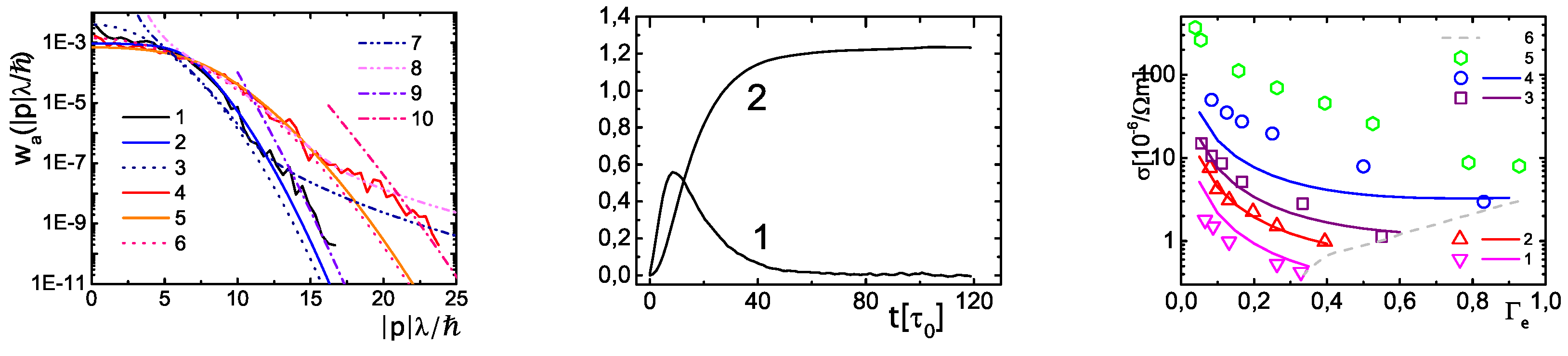
The WPIMC calculations for the electron and hole momentum distribution functions in electron - hole plasma are presented in Figure 1 (left panel) by Lines 1 and 4 for electrons and holes, respectively. Here, the parameter of electronic degeneracy is equal to four ($T/E_F=0.261$), while the hole mass is two times larger than the electron mass. Figure 1 also presents several related analytical dependencies: FD (Lines 2 and 5), MD (Lines 3 and 6), P8 (Lines 7 and 8), and P8MDEF (Lines 9 and 10).

Here, the constant in P8 and the effective temperature in P8MDEF have been used as the adjustable parameters to fit the WPIMC momentum distribution functions in the large momentum asymptotic regions.

Transport coefficients: A natural way to obtain transport coefficients is making use of the quantum Green–Kubo relations [12]. These relations give the transport coefficients in terms of integrals of equilibrium time-dependent correlation functions. According to Equation (8), the electron conductivity $\sigma$ is the integral of the velocity–velocity autocorrelation function

$$\begin{array}{c}\hfill {\sigma }_e=e^2{n}_e\beta \underset{t\to \infty }{lim}\frac{1}{3}{\int }_0^{t}d\tau {\langle v(0)·v(\tau )\rangle }_e\\ \hfill {\langle v(0)·v(\tau )\rangle }_e={(2\pi \hslash )}^{-2\nu }\int d\overline{pq}d\widetilde{pq}W\left(\overline{pq};\widetilde{pq};\tau ;\beta \right)v_e\left(\overline{p}(\tau )\right)·v_e\left(\tilde{p}(\tau )\right),\end{array}$$

(14)

where the scalar product of 3D-velocities is

$$\begin{array}{c}\hfill v_e\left(\overline{p}(\tau )\right)·v_e\left(\tilde{p}(\tau )\right)=\frac{1}{N_e}\sum _{i=1}^{N_e}\frac{{\overline{\mathbf{p}}}_i(\tau )·{\tilde{\mathbf{p}}}_i(\tau )}{m_i^2},\end{array}$$

(15)

and the trajectories in positive (bared) and inverse (tilded) time directions are defined by Equations (4) and (5), respectively.

Calculations of autocorrelation functions are performed in canonical ensemble and include combination of the Monte-Carlo sampling of initial conditions ${\overline{pq}}_0$ and ${\widetilde{pq}}_0$ for trajectories and solving the system of dynamic Hamiltonian Equations (4) and (5). The initial conditions ${\overline{pq}}_0$ and ${\widetilde{pq}}_0$ for the trajectories are sampled by Monte-Carlo method according to the modulus of probability $W^0\left({\overline{pq}}_0;{\widetilde{pq}}_0;\beta \right)$, while sign of the $W^0\left({\overline{pq}}_0;{\widetilde{pq}}_0;\beta \right)$ is accounted for as a wieght function at calculations average values [2].

First, we discuss the velocity–velocity autocorrelation function (VVACF). Figure 1 (central panel) shows examples of the velocity–velocity autocorrelation functions and its antiderivatives. The initial Wigner distribution ${\overline{W}}^0$, due to the path integral representation, accounts for momentum–coordinate principle uncertainty. Consequently, the initial momenta are to a great extent independent form each other and the VVACF approach to zero. Some time later, correlation of the VVACF starts to grow due to strong interaction with surrounding particles. This happens as ${\Gamma }_e\le 1$, $|\overline{q_0}-\widetilde{q_0}|\sim {\lambda }_e$ and ${\lambda }_e\le \beta e^2\le r_s{a}_B$ and the virtual trajectories $\overline{pq}$ and $\widetilde{pq}$ are approximately continuations of each other independently from initial conditions. Subsequent decay of the VVACF results from interaction with far particles at distances larger than $r_s$. According to Figure 1, the damping time of the VVACF turns out to be strongly affected by the variations of density and temperature.

Let us discuss now the conductivity of a strongly coupled Coulomb system. Figure 1 (right) presents comparison of our conductivity isochores with those obtained from the interpolation formula for conductivity of fully ionized hydrogen plasma derived in [26,27]. This figure demonstrates agreement of both data at low densities and high temperatures. Let us stress that Line 6 restricts approximately from above the region of conductivity sharp drop due to arising bound states of many particle clusters.

5. Discussion

In this work, we use the generalization of the classical molecular dynamics methods allowing to take into account quantum effects. We use the Feynman and Wigner formulations of quantum mechanics combining with Monte Carlo methods for numerical treatment of the kinetic properties of dense quantum plasma media. The Wigner–Liouville-like equation is solved by a combination of Wigner molecular dynamics (WMD) and by Monte-Carlo method in phase space (WPIMC) methods. The initial Wigner-like function has been presented in the form of path integrals. Fermi statistical effects are accounted for by effective pair pseudopotential depending on coordinates, momenta and degeneracy parameter of particles and taking into account Pauli blocking of fermions. WPIMC allows calculating thermodynamic quantities and pair distribution functions in a wide range of density and temperature.

Comparison of the classical Maxwell–Boltzmann and quantum Fermi–Dirac distribution shows the significant influence of the interparticle interaction on the high energy asymptotics of the momentum distribution functions resulting in appearance of the power-law quantum “tails”. To study the influence of the interparticle interaction on the dynamic properties of dense plasmas, we also compute the temporal correlation functions of quantum operators. According to the quantum Kubo formula, we determined the electron conductivity and compared obtained results with available theories. Our results show a strong dependence on the plasma parameters and for fully ionized plasma are in a agreement with available theories, simulations, experimental data and interpolation formula obtained by Esser, Redmer and Röpke. Appearance of bound states and many particle clusters in plasma results in sharp drop of electron conductivity.

References

- Weinbub, J.; Ferry, D.K. Recent advances in Wigner function approaches. Appl. Phys. Rev. 2018, 5, 041104. [Google Scholar] [CrossRef]
- Ebeling, W.; Fortov, V.; Filinov, V. Quantum Statistics of Dense Gases and Nonideal Plasmas; Springer: Berlin, Germany, 2017. [Google Scholar]
- Eleuch, H.; Ben Nessib, N.; Bennaceur, R. Quantum model of emission in a weakly non ideal plasma. Eur. Phys. J. D 2004, 29, 391–395. [Google Scholar] [CrossRef]
- Elabidi, H.; Ben Nessib, N.; Sahal-Bréchot, S. Quantum mechanical calculations of the electron-impact broadening of spectral lines for intermediate coupling. J. Phys. B At. Mol. Phys. 2004, 37, 63–71. [Google Scholar] [CrossRef]
- Ben Chaouacha, H.; Ben Nessib, N.; Sahal-Bréchot, S. Semi-classical collisional functions in a strongly correlated plasma. Astron. Astrophys. 2004, 419, 771–776. [Google Scholar] [CrossRef] [Green Version]
- Feynman, R.P.; Hibbs, A.R. Quantum Mechanics and Path Integrals; McGraw-Hill: New York, NY, USA, 1965. [Google Scholar]
- Dornheim, T.; Groth, S.; Filinov, A.; Bonitz, M. Permutation blocking path integral Monte Carlo: A highly efficient approach to the simulation of strongly degenerate non-ideal fermions. New J. Phys. 2015, 17, 073017. [Google Scholar] [CrossRef]
- Dornheim, T.; Groth, S.; Sjostrom, T.; Malone, F.D.; Foulkes, W.M.C.; Bonitz, M. Ab initio Quantum Monte Carlo simulation of the warm dense electron gas in the thermodynamic limit. Phys. Rev. Lett. 2016, 117, 156403. [Google Scholar] [CrossRef] [PubMed]
- Wigner, E.P. On the Quantum Correction For Thermodynamic Equilibrium. Phys. Rev. 1932, 40, 749–759. [Google Scholar] [CrossRef]
- Tatarskii, V. The Wigner representation of quantum mechanics. Sov. Phys. Uspekhi 1983, 26, 311–327. [Google Scholar] [CrossRef]
- Filinov, V.S.; Fehske, H.; Bonitz, M.; Fortov, V.E.; Levashov, P.R. Correlation effects in partially ionized mass asymmetric electron-hole plasmas. Phys. Rev. E 2007, 75, 036401. [Google Scholar] [CrossRef] [PubMed] [Green Version]
- Zubarev, D.N.; Morozov, V.; Ropke, G. Statistical Mechanics of Nonequilibrium Processes; Akademie Verlag-Wiley: Berlin, Germany, 1996. [Google Scholar]
- Filinov, V.; Medvedev, Yu.; Kamskii, V. Quantum dynamics and Wigner representation of quantum mechanics. J. Mol. Phys. 1995, 85, 711–726. [Google Scholar] [CrossRef]
- Filinov, V.S. Wigner approach to quantum statistical mechanics and quantum generalization of molecular dynamics method. Part I. J. Mol. Phys. 1996, 88, 1517–1528. [Google Scholar] [CrossRef]
- Filinov, V.S. Wigner approach to quantum statistical mechanics and quantum generalization of molecular dynamics method. Part II. J. Mol. Phys. 1996, 88, 1529–1539. [Google Scholar] [CrossRef]
- Wiener, N. Differential-Space. J. Math. Phys. 1923, 2, 131–174. [Google Scholar] [CrossRef]
- Kelbg, G. Theorie des Quanten-Plasmas. Ann. Phys. 1963, 457, 354. [Google Scholar] [CrossRef]
- Ebeling, W.; Hoffmann, H.J.; Kelbg, G. Quantenstatistik des Hochtemperatur-Plasmas im thermodynamischen Gleichgewicht. Contrib. Plasma Phys. 1967, 7, 233–248. [Google Scholar] [CrossRef]
- Galitskii, V.M.; Yakimets, V.V. Particle relaxation in a Maxwell gas. J. Exp. Theor. Phys. 1966, 51, 957–964. [Google Scholar]
- Kimball, J. Short-range correlations and the structure factor and momentum distribution of electrons. J. Phys. A Math. Gen. 1975, 8, 1513. [Google Scholar] [CrossRef]
- Starostin, A.N.; Mironov, A.B.; Aleksandrov, N.L.; Fisch, N.J.; Kulsrud, R.M. Quantum corrections to the distribution function of particles over momentum in dense media. Phys. A 2002, 305, 287–296. [Google Scholar] [CrossRef]
- Eletskii, A.V.; Starostin, A.N.; Taran, M.D. Quantum corrections to the equilibrium rate constants of inelastic processes. Phys. Uspekhi 2005, 48, 281–294. [Google Scholar] [CrossRef]
- Emelianov, A.V.; Eremin, A.V.; Petrushevich, Y.V.; Sivkova, E.E.; Starostin, A.N.; Taran, M.D.; Fortov, V.E. Quantum effects in the kinetics of the initiation of detonation condensation waves. JETP Lett. 2011, 94, 530–534. [Google Scholar] [CrossRef]
- Kochetov, I.V.; Napartovich, A.P.; Petrushevich, Y.V.; Starostin, A.N.; Taran, M.D. Calculation of thermal ignition time of hydrogen–air mixtures taking into account quantum corrections. High Temp. 2016, 54, 563–540. [Google Scholar] [CrossRef]
- Starostin, A.N.; Petrushevich, Y.V. Scientific-Coordination Workshop on Non-Ideal Plasma Physics. 7–8 December 2016, Moscow, Russia. Available online: http://www.ihed.ras.ru/npp2016/program (accessed on 22 November 2018).
- Esser, A.; Redmer, R.; Röpke, G. Interpolation formula for the electrical conductivity of nonideal plasmas. Contrib. Plasma Phys. 2003, 43, 33–38. [Google Scholar] [CrossRef] [Green Version]
- Adams, J.R.; Shilkin, N.S.; Fortov, V.E.; Gryaznov, V.K.; Mintsev, V.B.; Redmer, R.; Reinholz, H.; Röpke, G. Coulomb contribution to the direct current electrical conductivity of dense partially ionized plasmas. Phys. Plasmas 2007, 14, 062303. [Google Scholar] [CrossRef]
Figure 1.
(Color online) (Left) The momentum distribution functions for interacting electrons and two times heavier holes. The electronic momentum distributions are presented by Lines 1, 2, 3, 7, and 9, while analogous results for holes are presented by Lines 4, 5, 6, 8, and 10. The physical meaning of these lines is given in text. Degeneracy of electrons is equal to 4 (), while and the plasma classical coupling parameter is equal to 2. (Central) The velocity–velocity autocorrelation function (Line 1) and its antiderivative function (Line 2) versus time in atomic units () for , . (Right) Electrical electron conductivity as function of the coupling parameter for different fixed densities of two component Coulomb system. Empty scatters 1–5 show results of this work for the fixed , respectively, while related lines present results of interpolation formula for conductivity of fully ionized hydrogen plasma [26,27]. Line 6 restricts approximately from above the region of conductivity sharp drop due to arising bound states of many particle clusters.
© 2018 by the authors. Licensee MDPI, Basel, Switzerland. This article is an open access article distributed under the terms and conditions of the Creative Commons Attribution (CC BY) license (http://creativecommons.org/licenses/by/4.0/).
Share and Cite
MDPI and ACS Style
Filinov, V.; Larkin, A. Quantum Dynamics of Charged Fermions in the Wigner Formulation of Quantum Mechanics. Universe 2018, 4, 133. https://doi.org/10.3390/universe4120133
AMA Style
Filinov V, Larkin A. Quantum Dynamics of Charged Fermions in the Wigner Formulation of Quantum Mechanics. Universe. 2018; 4(12):133. https://doi.org/10.3390/universe4120133
Chicago/Turabian StyleFilinov, Vladimir, and Alexander Larkin. 2018. "Quantum Dynamics of Charged Fermions in the Wigner Formulation of Quantum Mechanics" Universe 4, no. 12: 133. https://doi.org/10.3390/universe4120133
Note that from the first issue of 2016, this journal uses article numbers instead of page numbers. See further details here.