Using Trajectories in Quantum Cosmology

Simple Summary

I discuss the application of quantum trajectory formalism to the FLRW Universe.

Abstract

Quantum cosmology based on the Wheeler De Witt equation represents a simple way to implement plausible quantum effects in a gravitational setup. In its minisuperspace version wherein one restricts attention to FLRW metrics with a single scale factor and only a few degrees of freedom describing matter, one can obtain exact solutions and thus acquire full knowledge of the wave function. Although this is the usual way to treat a quantum mechanical system, it turns out however to be essentially meaningless in a cosmological framework. Turning to a trajectory approach then provides an effective means of deriving physical consequences.

1. Introduction

Quantum cosmology [1,2] aims at understanding how gravitational fields describing cosmological setups, usually treated as purely classical backgrounds [3], may be affected by quantization. In particular, the most important issue not addressed by classical general relativity, i.e., the singularity from which our Universe ensues, could be tackled by imposing physically relevant boundary conditions on the wave function.

The Universe being by definition unique, and quantum measurements being understood by means of ensemble averages, i.e., repeated experiments, the meaning of the wave function of the Universe seems rather unclear. There exists however a formulation of quantum mechanics, originally developed by de Broglie [4] and Bohm [5,6] and based on trajectories [7] that, as it happens, is easily applicable to cosmology [8]. It is in this framework that one can assign actual values at each instant of time to the scale factor (the quantum trajectory) [9,10] and even address the question of time [11].

In the following, I briefly recap how gravitation may be quantized à la Wheeler De Witt and how does the restriction to Friedmann-Lemaître-Roberston-Walker (FLRW) minisuperspace provides a time-dependent Schrödinger-like equation when a perfect fluid is considered to be the source of Einstein equations. The trajectory approach then permits to derive a fully quantum time-dependent scale factor whose properties are examined in detail.

2. General Setup

2.1. Classical Hamiltonian General Relativity

Since the purpose is to quantize general relativity (GR) [12], one starts from the usual Einstein-Hilbert action on a compact space $\mathcal{M}$ with boundary $\partial \mathcal{M}$, including a possible cosmological constant $\mathsf{\Lambda }$,

$$\mathcal{S}=\frac{1}{16\pi G_{{}_{\mathrm{N}}}}\left[{\int }_{\mathcal{M}}\sqrt{-g}\left(R-2\mathsf{\Lambda }\right){\mathrm{d}}^{4}x+2{\int }_{\partial \mathcal{M}}\sqrt{h}{K}_i^i{\mathrm{d}}^{3}x\right]+{\mathcal{S}}_{\mathrm{matter}}\left[\mathsf{\Phi }\left(x\right)\right],$$

(1)

where the Ricci scalar R is coupled to matter fields symbolically named $\mathsf{\Phi }$. Figure 1 shows the usual 3+1 split of spacetime when the metric takes the form

$$\mathrm{d}{s}^2=g_{\mu \nu }\mathrm{d}{x}^{\mu }\mathrm{d}{x}^{\nu }=-N^2\mathrm{d}{t}^2+h_{ij}\left(\mathrm{d}{x}^i+N^i\mathrm{d}t\right)\left(\mathrm{d}{x}^j+N^j\mathrm{d}t\right).$$

(2)

In (1), the extrinsic curvature of each leaf ${\mathsf{\Sigma }}_t$ is given by

$$K_{ij}=-{\nabla }_j^{\left(h\right)}{n}_i=\frac{1}{2N}\left({\nabla }_j^{\left(h\right)}{N}_i+{\nabla }_i^{\left(h\right)}{N}_j-\frac{\partial h_{ij}}{\partial t}\right),$$

(3)

where ${\nabla }^{\left(h\right)}$ is the covariant derivative associated with the intrinsic metric $h_{ij}$. From

$$\mathcal{S}=\int L\mathrm{d}t=\frac{1}{16\pi G_{{}_{\mathrm{N}}}}\int \mathrm{d}t\left[\int {\mathrm{d}}^{3}xN\sqrt{h}\left(K_{ij}{K}^{ij}-K^2+{}^{3}R-2\mathsf{\Lambda }\right)+L_{\mathrm{matter}}\right],$$

(4)

one derives the canonical momenta

$${\pi }^{ij}\equiv \frac{\delta L}{\delta {\dot{h}}_{ij}}=-\frac{\sqrt{h}}{16\pi G_{{}_{\mathrm{N}}}}\left(K^{ij}-h^{ij}K\right),{\pi }^0\equiv \frac{\delta L}{\delta \dot{N}}=0,{\pi }^i\equiv \frac{\delta L}{\delta \dot{N^i}}=0,$$

(5)

the last two providing primary constraints, as well as the momentum associated with the matter component, ${\pi }^{\mathsf{\Phi }}$ say. The Hamiltonian is therefore

$$H\equiv \int {\mathrm{d}}^{3}x\left({\pi }^0\dot{N}+{\pi }^i{\dot{N}}_i+{\pi }^{ij}{\dot{h}}_{ij}+{\pi }^{\mathsf{\Phi }}\dot{\mathsf{\Phi }}\right)-L=\int {\mathrm{d}}^{3}x\left({\pi }^0\dot{N}+{\pi }^i{\dot{N}}_i+NH+N_i{\mathcal{H}}^i\right).$$

(6)

Variations of (6) yields the Hamiltonian description of GR.

2.2. Quantization

Quantum mechanics proceeds by first defining a Hilbert space of accessible states. In the GR case, it is the space of all the 3-metrics $h_{ij}$ and matter fields compatible with diffeomorphism invariance; it is called superspace. The wave functional is then $\mathsf{\Psi }\left[h_{ij}\left(x\right),\mathsf{\Phi }\left(x\right)\right]$ and depends on the coordinates $\left\{x^{\mu }\right\}$, now understood as mere parameters.

Upon adopting the Dirac canonical quantization procedure whereby canonical momenta are replaced by $-i$ times the functional derivative with respect to the variable they are the momenta of, i.e.,

$${\pi }^{ij}\to -i\frac{\delta }{\delta h_{ij}},{\pi }^0\to -i\frac{\delta }{\delta N},{\pi }^i\to -i\frac{\delta }{\delta N_i},{\pi }^{\mathsf{\Phi }}\to -i\frac{\delta }{\delta \mathsf{\Phi }},$$

(7)

one finds that the primary constraints translate into the fact that the wave function depends neither on the lapse function nor on the shift vector, that it is unchanged under diffeomorphisms, and finally that the Wheeler De Witt equation

$$H\mathsf{\Psi }=\left[-16\pi G_{{}_{\mathrm{N}}}{\mathcal{G}}_{ijkl}\frac{{\delta }^2}{\delta h_{ij}\delta h_{kl}}+\frac{\sqrt{h}}{16\pi G_{{}_{\mathrm{N}}}}\left({-}^{3}R+2\mathsf{\Lambda }+16\pi G_{{}_{\mathrm{N}}}{\widehat{T}}^{00}\right)\right]\mathsf{\Psi }=0$$

(8)

holds, with the De Witt metric defined as

$${\mathcal{G}}_{ijkl}=\frac{1}{2\sqrt{h}}\left(h_{ik}{h}_{jl}+h_{il}{h}_{jk}-h_{ij}{h}_{kl}\right),$$

(9)

and ${}^{3}R$ is the curvature associated with the metric $h_{ij}$. In (8), $\widehat{\mathit{T}}$ is the operator version on superspace of the stress energy tensor relevant for the matter fields.

2.3. Minisuperspace

As it is essentially out of question to solve (8) in general, one restricts attention to the special FLRW case for which one replaces the general 3D metric $h_{ij}$ by

$$h_{ij}\mathrm{d}{x}^i\mathrm{d}{x}^j\mapsto a^2\left(t\right)\left[\frac{\mathrm{d}{r}^2}{1-\mathcal{K}{r}^2}+r^2\left(\mathrm{d}{\theta }^2+{sin}^2\theta \mathrm{d}{\varphi }^2\right)\right],$$

(10)

leading to a numerical parameter, the spatial curvature $\mathcal{K}$, in practice set to zero in agreement with observational data, and a dynamical function, the scale factor $a\left(t\right)$. Under the assumption that the 3D metric takes the form (10), the Wheeler De Witt equation becomes a Schrödinger-like equation for, say, the 2 degrees of freedom wave function $\mathsf{\Psi }\left[a\left(t\right),\varphi \left(t\right)\right]$. There are many points, both mathematical and physical, that can be raised about the minisuperspace approach, but they shall not concern us in the framework of this paper, and we refer the reader to, for instance, Refs. [8,13] and the references therein for that matter.

We want instead here focus on the simplest possibility, namely that of vanishing spatial curvature $\mathcal{K}\to 0$ and consider as the matter component a perfect fluid which we treat using Schutz formalism [14,15]. In this formalism, the full Hamiltonian reads

$$\mathrm{d}{s}^2=N^2\left(\tau \right)\mathrm{d}\tau -a^2\left(\tau \right){\gamma }_{ij}\mathrm{d}{x}^i\mathrm{d}{x}^j\mathrm{and}p=w\rho ⟹H=N\left(-\frac{{\pi }_a^2}{4a}+\frac{{\pi }_t}{a^{3w}}\right),$$

(11)

where the variable t is associated to the velocity potentials and we keep the lapse function $N\left(\tau \right)$ unfixed for later convenience. With the choice $N\to a^{3w}$ and for a radiation fluid having $w=\frac{1}{3}$, the replacement ${\pi }_t\to -i{\partial }_t$ transforms the Wheeler De Witt equation $H\mathsf{\Psi }=0$ into $i{\partial }_t\mathsf{\Psi }=\frac{1}{4}{\partial }_a^2\mathsf{\Psi }$, which is, up to a sign, a time-dependent Schrödinger equation for a free particle [9]. Not surprisingly, the fluid has permitted to define a global time variable.

3. Quantum Trajectories

Although it is not the purpose of this paper to review the trajectory method in quantum mechanics, let me summarize it shortly.

Since we have seen that the matter content merely serves in our case to define a time variable in the time-dependent Schrödinger equation, I now consider a canonical transformation for the scale factor, namely $\left(a,{\pi }_a\right)\mapsto \left(A,{\mathsf{\Pi }}_A\right)$, leading to $H\left(a,{\pi }_a\right)\mapsto \mathcal{H}\left(A,{\mathsf{\Pi }}_A\right)$ by means of a generating function $F(a,A;t)$ satisfying

$$\dot{a}{\pi }_a-H=\dot{A}{\mathsf{\Pi }}_A-\mathcal{H}+\frac{\mathrm{d}F}{\mathrm{d}t}⟹\mathrm{d}F={\pi }_a\mathrm{d}a-{\mathsf{\Pi }}_A\mathrm{d}A+\left(\mathcal{H}-H\right)\mathrm{d}t.$$

(12)

From (12), one infers that

$$\mathrm{d}\left(F+A{\mathsf{\Pi }}_A\right)={\pi }_a\mathrm{d}a+A\mathrm{d}{\mathsf{\Pi }}_A+\left(\mathcal{H}-H\right)\mathrm{d}t,$$

(13)

showing that the function $\left(F+A{\mathsf{\Pi }}_A\right)$ depends on a, ${\mathsf{\Pi }}_A$ and t.

We now choose the canonical transformation such that the new Hamiltonian $\mathcal{H}$ identically vanishes on shell. Hamilton equations then imply

$$\dot{A}=\frac{\partial \mathcal{H}}{\partial {\mathsf{\Pi }}_A}=0\mathrm{and}{\dot{\mathsf{\Pi }}}_A=-\frac{\partial \mathcal{H}}{\partial A}=0⟹\frac{\mathrm{d}\left(F+A{\mathsf{\Pi }}_A\right)}{\mathrm{d}t}=\dot{a}{\pi }_a-H=L,$$

L being the original Lagrangian [see Equation (4)]. Therefore, one may identify the function $\left(F+A{\mathsf{\Pi }}_A\right)$ with the action $\mathcal{S}=\int L\mathrm{d}t$. Equation (13), taken on shell, now reads

$$\mathrm{d}\mathcal{S}={\pi }_a\mathrm{d}a-H\mathrm{d}t⟹\frac{\partial \mathcal{S}}{\partial t}=-H\mathrm{and}\frac{\partial \mathcal{S}}{\partial a}={\pi }_a,$$

(14)

which can be recast in the more usual Hamilton-Jacobi form

$$H\left(a,\frac{\partial \mathcal{S}}{\partial a}\right)+\frac{\partial S}{\partial t}=0,$$

(15)

and the last equation of (14) relates the actual value of the momentum to the gradient of the action; as we shall see below, this will be equivalent to the pilot-wave equation when the action is identified with the phase of the wave function.

In a quantum framework, the modified Hamilton-Jacobi equation is obtained as the real part of the Schrödinger equation when the wave function is written explicitly as an amplitude $R\in \mathbb{R}$ and a phase $S\in \mathbb{R}$, namely when setting $\mathsf{\Psi }(a,t)=R{\mathrm{e}}^{iS}$. This is one way to identify the phase of the wave function with the action. As a result, it is natural to assume that an actual trajectory can be obtained as the solution of the canonical transformation eikonal relation ${\pi }_a{|}_{\mathrm{actual}}\propto \dot{a}=\partial S/\partial a$, the dot denoting a time derivative.

It is instructive to note as well that setting $\rho =R^2$ and replacing the time derivative $\dot{a}$ by an actual velocity v, one finds that the imaginary part of Schrödinger equation may be written as

$$\frac{\partial \rho }{\partial t}+\mathrm{div}\left(\rho v\right)=0,$$

where the divergence is with respect to the variable a. In other words, this formulation of quantum physics is very close to ordinary fluid mechanics, and the same methods (Eulerian or Lagrangian) actually apply.

Solving the trajectory equation is all but trivial, and many methods, mostly numerical, have been devised [16]. The one we use in the examples presented below is based on a simple radial basis interpolation, but it can be extended to include a moving mesh method. In fact, if the initial distribution of points $\left\{a_n{|}_{t=t_0}\right\}$ at which the trajectories are calculated is ${\left|\mathsf{\Psi }\right|}^2$, then it remains distributed along the square of the wave function at all subsequent times, so that whatever the behavior of $\mathsf{\Psi }$, one is sure to cover a domain that always remains where the wave function is large. For our illustrative purpose however, this refinement is not necessary.

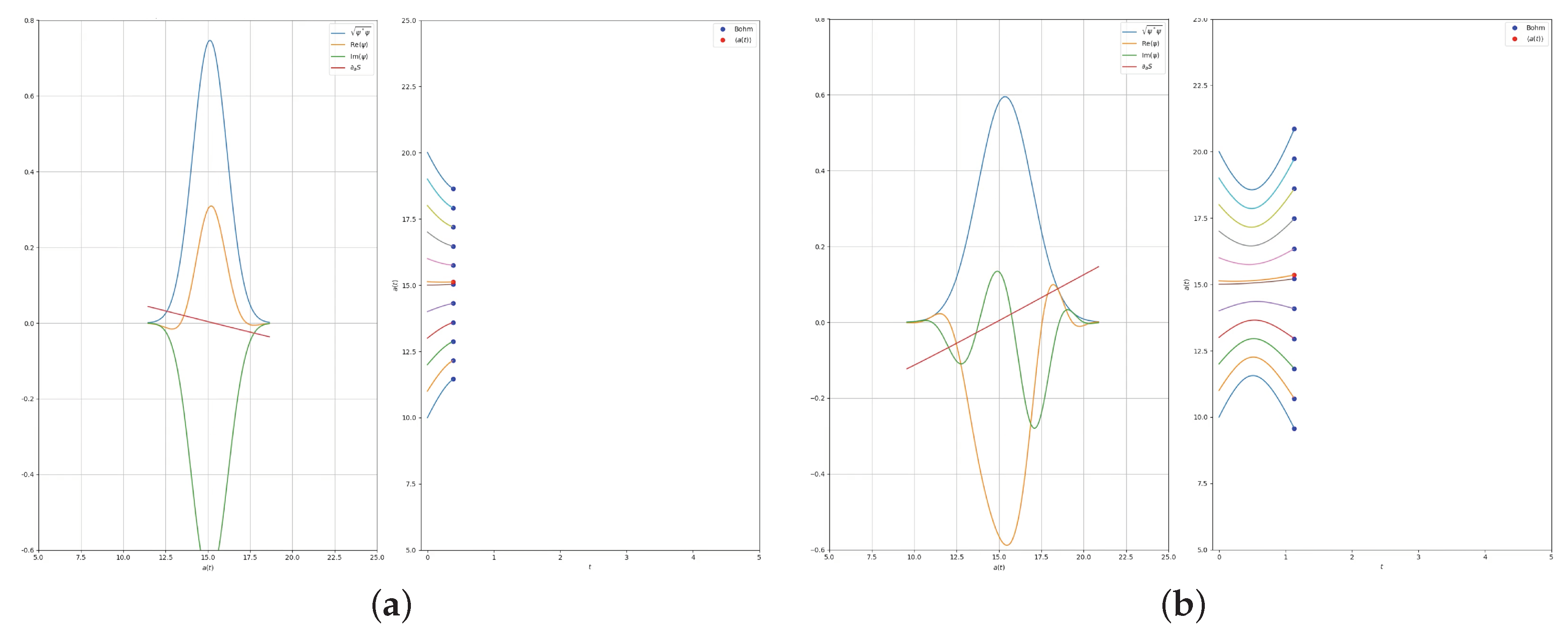
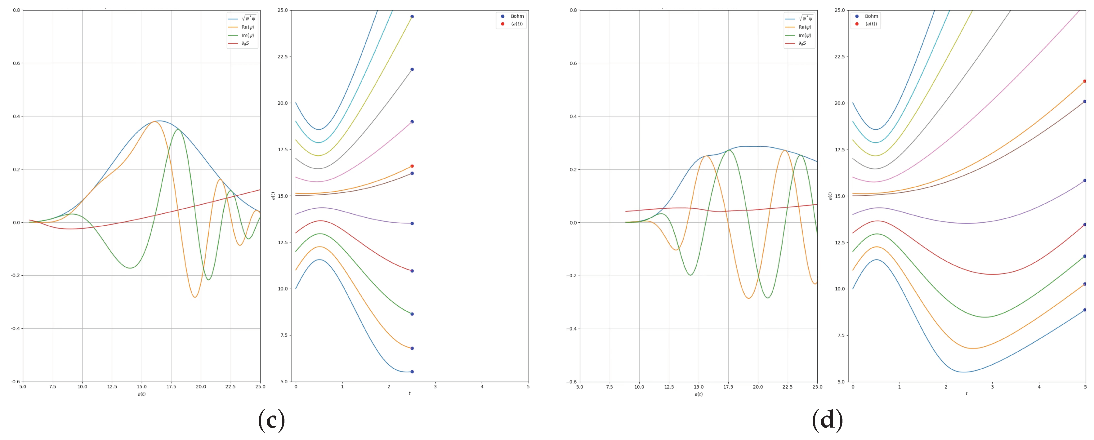
In most cases of cosmological relevance, even if one wants to compare the canonical quantization procedure with less usual ones [17], or even when a larger minisuperspace is considered, e.g., to account for a possible anisotropy (Bianchi Universe) [10], one ends up essentially solving a Schrödinger equation in a potential. Figure 2 exemplifies a particular case, showing the real and imaginary parts of the wave function, its amplitude, and the derivative of its phase with respect to the scale factor. It illustrates that not only is the singularity resolved by quantum mechanics effects in this approach, but that the resulting actual trajectory depends crucially on the initial condition of the scale factor.

4. Conclusions

The trajectory method, also known as de Broglie Bohm pilot wave, permits a clearer understanding of how quantum effects may affect cosmology near the singularity, resolving the latter. However, it also shows that defining the state itself may not be sufficient, as the initial condition fixes the subsequent evolution of the scale factor: it may bounce once or many times depending on its initial value! If one calculates perturbations in a self-consistent way [18] on top of such a trajectory, they will depend explicitly on which trajectory has been chosen. This could actually provide a means of measuring the time evolution of the very early scale factor.

References

- Halliwell, J.J. Introductory Lectures on Quantum Cosmology. In Proceedings of the 7th Jerusalem Winter School for Theoretical Physics: Quantum Cosmology and Baby Universes, Jerusalem, Israel, 27 December 1989–4 January 1990; pp. 159–243. [Google Scholar]
- Bojowald, M. Quantum cosmology: A review. Rept. Prog. Phys. 2015, 78, 023901. [Google Scholar] [CrossRef] [PubMed]
- Peter, P.; Uzan, J.P. Primordial Cosmology; Oxford Graduate Texts; Oxford University Press: Oxford, UK, 2013. [Google Scholar]
- De Broglie, L.V.P.R. Recherches sur la théorie des quanta. Ann. Phys. 1925, 2, 22–128. [Google Scholar] [CrossRef]
- Bohm, D. A Suggested interpretation of the quantum theory in terms of hidden variables. 1. Phys. Rev. 1952, 85, 166–179. [Google Scholar] [CrossRef]
- Bohm, D. A Suggested interpretation of the quantum theory in terms of hidden variables. 2. Phys. Rev. 1952, 85, 180–193. [Google Scholar] [CrossRef]
- Holland, P.R. The de Broglie-Bohm theory of motion and quantum field theory. Phys. Rep. 1993, 224, 95–150. [Google Scholar] [CrossRef]
- Pinto-Neto, N.; Fabris, J.C. Quantum cosmology from the de Broglie-Bohm perspective. Class. Quant. Grav. 2013, 30, 143001. [Google Scholar] [CrossRef]
- Acacio de Barros, J.; Pinto-Neto, N.; Sagioro-Leal, M.A. The Causal interpretation of dust and radiation fluids nonsingular quantum cosmologies. Phys. Lett. 1998, A241, 229–239. [Google Scholar] [CrossRef]
- Peter, P.; Vitenti, S.D.P. The simplest possible bouncing quantum cosmological model. Mod. Phys. Lett. 2016, A31, 1640006. [Google Scholar] [CrossRef]
- Acacio de Barros, J.; Pinto-Neto, N. The causal interpretation of quantum mechanics and the singularity problem and time issue in quantum cosmology. Int. J. Mod. Phys. 1998, D7, 201–213. [Google Scholar] [CrossRef]
- Kiefer, C. Quantum Gravity; Oxford University Press: New York, NY, USA, 2007. [Google Scholar]
- Kiefer, C. Conceptual Issues in Canonical Quantum Gravity and Cosmology. In Proceedings of the 2nd International Conference, Novosibirsk, Russia, 26–31 August 2007; University of Nova Gorica Press: Nova Gorica, Slovenia, 2008; pp. 131–143. [Google Scholar]
- Schutz, B. Perfect Fluids in General Relativity: Velocity Potentials and a Variational Principle. Phys. Rev. D 1970, 2, 2762. [Google Scholar] [CrossRef]
- Schutz, B. Hamiltonian Theory of a Relativistic Perfect Fluid. Phys. Rev. D 1971, 4, 3559. [Google Scholar] [CrossRef]
- Wyatt, R.E. Quantum Dynamics with Trajectories. Introduction to Quantum Hydrodynamics; Springer Science & Business Media: Berlin, Germany, 2005; Volume 28. [Google Scholar]
- Bergeron, H.; Gazeau, J.P.; Małkiewicz, P. Primordial gravitational waves in a quantum model of big bounce. JCAP 2018, 1805, 057. [Google Scholar] [CrossRef]
- Peter, P.; Pinto-Neto, N. Cosmology without inflation. Phys. Rev. 2008, D78, 063506. [Google Scholar] [CrossRef]
Figure 1.
(a) Spacetime foliation in terms of hypersurfaces , each labelled by a time-like parameter t. The diagram defines the normal and makes explicit the decomposition of a tangent to the worldline through the lapse function N and shift vector . (b) A time-evolved example with a few typical trajectories showing a quantum non-singular bouncing universe.
Figure 2.
Time evolution of a wave function and typical trajectories: (a) initial condition, the phase gradient has both positive and negative values, so some trajectories are expanding while other are contracting, depending on their initial value. (b) An instant later, the phase gradient has essentially reversed, so all trajectories have bounced in one way or another. (c) After some time, the phase gradient tends to increase to become almost everywhere positive. (d) Finally, the Universe starts expanding forever. Also shown is the average value of the scale factor, which is seen to be potentially very different from the typical trajectories (and it is not even the same as the trajectory having the same initial value of a, i.e., that for which a(t0) = 〈a〉).
© 2018 by the author. Licensee MDPI, Basel, Switzerland. This article is an open access article distributed under the terms and conditions of the Creative Commons Attribution (CC BY) license (http://creativecommons.org/licenses/by/4.0/).
Share and Cite
MDPI and ACS Style
Peter, P. Using Trajectories in Quantum Cosmology. Universe 2018, 4, 89. https://doi.org/10.3390/universe4080089
AMA Style
Peter P. Using Trajectories in Quantum Cosmology. Universe. 2018; 4(8):89. https://doi.org/10.3390/universe4080089
Chicago/Turabian StylePeter, Patrick. 2018. "Using Trajectories in Quantum Cosmology" Universe 4, no. 8: 89. https://doi.org/10.3390/universe4080089
APA StylePeter, P. (2018). Using Trajectories in Quantum Cosmology. Universe, 4(8), 89. https://doi.org/10.3390/universe4080089
Note that from the first issue of 2016, this journal uses article numbers instead of page numbers. See further details here.