1. Introduction
In cosmology we know that the Universe is not perfectly homogeneous and isotropic but rather comprises of fluctuations, in matter density and in temperature, which are congregated and correlated in a rather specific manner. Detailed measurements of these fluctuations can be characterized by correlation functions and power spectra [
1,
2,
3,
4,
5,
6,
7,
8,
9,
10]. The question of why these fluctuations are distributed the way they are is thus an important one in cosmology. The conventional explanation of the shape of these power spectra is provided by inflation, which is based on the hypothesis of additional primordial scalar fields called inflatons [
11,
12,
13]. The shape of the power spectrum is thus derived from quantum fluctuation of these primordial inflaton fields, and the agreement of this prediction with observations to high accuracy has been widely regarded as a great triumph and confirmation for inflation [
14].
In our previous work [
15], we have offered an alternative explanation based on gravitational fluctuations alone without inflation, which to our knowledge is the first-of-its-kind. While the short-distance theory of quantum gravity may still be highly uncertain due to both the flexibility of higher-order operators consistent with general covariance and the lack of experimental results, the long-distance or infrared limit of the theory is however in principle well-defined and unique, governed largely by the concept of universality. Although this long-distance quantum theory of gravity still suffers from being perturbatively nonrenormalizable, well known field theory techniques have been extensively developed, applied and tested in many other fields of physics where perturbation theory fails, usually due to a non-trivial vacuum structure. As a result, it is thus conceivable that these nonperturbative methods may find use in deriving physical consequences of perturbatively non-renormalizable theories such as gravity. Previous efforts [
16,
17] have shown that many such effects may manifest themselves and become important on very large cosmological scales. In particular, we found that much of the matter power spectrum can be derived and reproduced from Einstein gravity and standard
CDM cosmology alone, utilizing nonperturbative quantum field methods, without the need of additional scalar fields as advocated by inflation. We have shown that not only the predictions agree quite well with recent data, but also that additional quantum effects predict subtle deviations from the classical picture, which may become testable in the near future.
In this paper, we further investigate consequences from the above picture. Most importantly, we translate our quantum gravity prediction of the matter wavenumber power spectrum
to a prediction for the angular temperature power spectrum coefficients
’s. The angular temperature power spectrum, which expresses the power as coefficients of spherical harmonics (instead of plane waves, like the matter power spectrum) serves as a more direct comparison with observation, since after all the CMB measurements are performed over the sky. Unsurprisingly, we again find a general agreement between the observations and the gravitationally motivated prediction. Furthermore, additional quantum gravitational effects are expected to affect the low-
l regime of the
spectrum. As discussed in [
15], new quantum effects become significant when the separation-distances
r become comparable to a characteristic vacuum condensate scale of gravity
, which is expected to be extremely large (∼
), affecting very small
l’s in angular harmonic space. The additional quantum effects include the infrared (IR) regulator effects from the gravitational vacuum condensate and the renormalization group (RG) running of Newton’s constant
G. Here these effects on the angular spectrum are studied, and we show the occurrence of a dip in power in the low-
l regime. Furthermore, we argue that this may potentially be the cause for the well-known
anomaly in the
spectrum. Although it is impossible to make conclusive statements so far due to the large cosmic variance in that region, one might hope that there may be incremental improvements in systematic and experimental uncertainties in the near future, or that certain statistical likelihood-arguments for this effect can be made.
In addition, a number of updates will be presented here. In particular, new data sets of the matter power spectrum
have been released by the Planck collaboration [
18], very shortly after the publication of our first results and predictions. It is interesting here to study the consistency and improvements, if any, of the data. We find that the refined analyses and results not only remain consistent with our theoretical result, but a new point was published in [
18], which seems to suggest a downwards dip on the spectrum at low-
k, as a running Newton’s constant due to quantum gravity would suggest. Although the error bars on the points are too large to make conclusive statements, this remains an interesting development to study.
It is also possible to utilize these latest cosmological observations to constrain the theoretical values of the microscopic parameters, and thus further shed insight into the underlying theory. A handful of parameters in the theory are investigated, including the universal critical scaling exponent , the coefficient for the amplitude of quantum effects , and the characteristic nonperturbative correlation length scale . Our analyses show that while the latter ( and ) may only be constrained up to an order of magnitude, the data actually puts rather stringent constraints on the universal scaling exponent .
Finally, we present a study of the effect of the RG running of Newton’s constant
G derived from a recent alternative analytical nonperturbative approach—the Hartree-Fock (HF) approximation [
19]—on the power spectra. We find that these results predict the same general indication of a decrease in the power spectrum amplitude at scales close to the characteristic scale
, a behavior which is consistent with the predictions from other nonperturbative methods such as the Regge-Wheeler lattice formulation and the
dimensional expansion results. However the HF approximation seems to eventually predict an upturn in power at extreme low-
k regime and diverge from the other methods, which presumably indicates the limit of validity for this particular approximation method.
The paper is organized as follows.
Section 2 serves to outline the key points and results from the quantum theory of gravity and the resulting non-trivial scaling dimensions.
Section 3 summarizes the main results in deriving the power spectrum from quantum gravity. This section also includes updated plots with the latest results from experiments, and updated error bars.
Section 4 and
Section 5 investigate the possibility of constraining the theoretical scaling parameters from cosmology.
Section 6 relates the predictions on the matter power spectrum
to the angular temperature spectrum
’s, and the effects of an RG running of Newton’s constant
G on the
’s.
Section 7 discusses, summarizes and contrasts the current quantum gravity motivated picture with that of inflation, in view of explaining the measured power spectra. The section concludes by outlining a number of future issues of interest to this study.
2. Nonperturbative Approach to Quantum Gravity
Many more details on the nonperturbative approach to quantum gravity used in this paper can be found in a number of earlier works [
16,
17], and many references therein. The current section will therefore only serve to summarize the key points and main results which will become relevant for the subsequent discussion.
Quantum gravity, in essence the covariantly quantized theory of a massless spin-two particles, is in principle a unique theory, as shown by Feynman some time ago [
20,
21], much like Yang-Mills theory and QED are for massless spin-one particles. In the covariant Feynman path integral approach, only two key ingredients are needed to formulate the quantum theory—the gravitational action
and the functional measure over metrics
, leading to the generating function
where all physical observables could in principle be derived from. For gravity the action is given by the Einstein-Hilbert term augmented by a cosmological constant
where
R is the Ricci scalar,
g being the determinant of the metric
,
G Newton’s constant, and
the scaled cosmological constant (where a lower case is used here, as opposed to the more popular upper case in cosmology, so as not to confuse it with the ultraviolet-cutoff in quantum field theories that is commonly associated with
). The other key ingredient is the functional measure for the metric field, which in the case of gravity describes an integration over all four metrics, with weighting determined by the celebrated DeWitt form [
22].
There are two important subtleties worth noting here. Firstly, in principle, additional higher derivative terms that are consistent with general covariance could be allowed in the action, but nevertheless will only affect the physics at very short distances and will not be necessary here for studying large-distance cosmological effects. Secondly, as in most cases that the Feynman path integral can be written down, from non-relativistic quantum mechanics to field theories, the formal definition of integrals requires the introduction of a lattice, in order to properly account for, the known fact that quantum paths are nowhere differentiable. It is therefore a remarkable aspect that, at least in principle, the theory, in a nonperturbative context, does not seem to require any additional extraneous ingredients, besides the standard ones mentioned above, to properly define a quantum theory of gravity.
At the same time, gravity does present some rather difficult and fundamentally inherent challenges, such as the perturbatively nonrenormalizable nature due to a badly divergent series in Newton’s constant G, the intensive computational power required from being a highly nonlinear theory, the conformal instability which makes the Euclidean path integral potentially divergent, and further genuinely gravitational technical complications arising from the fact that physical distances between spacetime points, which depend on the metric which is a quantum entity, fluctuate.
Although these hurdles will ultimately need to be addressed in a complete and satisfactory way, a comprehensive account is of course far beyond the scope of this paper. However, regarding the perturbatively nonrenormalizable nature, some of the most interesting phenomena in physics often stem from non-analytic behavior in the coupling constant and the existence of nontrivial quantum condensates, which are hidden and impossible to probe within perturbation theory. It is therefore possible that challenges encountered in the case of gravity are more likely the result of inadequate calculational treatments, and not necessarily a reflection of some fundamentally insurmountable problem with the theory itself. Here, we shall take this as a motivation to utilize the plethora of well-established nonperturbative methods to deal with other quantum field theories where perturbation theory fails, and attempt to derive sensible physical predictions that can hopefully be tested against observations. More detailed accounts on the various issues associated with the theory of quantum gravity can be found for example in [
16,
17], and references therein.
For the present discussion, we will mention that the nonperturbative treatment of quantum gravity via Wilson’s
double expansion (in
G and the dimension) and the Regge-Wheeler lattice path integral formulation [
23] both reveal the existence of a new quantum phase, involving a nontrivial gravitational vacuum condensate [
16]. Along with this comes a nonperturbative characteristic correlation length scale,
, and a new set of non-trivial scaling exponents, as is common for well-studied perturbatively non-renormalizable theories
[
24,
25,
26,
27,
28,
29,
30,
31,
32,
33,
34]. Together, these two parameters characterize quantum corrections to physical observables such as the long-distance behavior of invariant correlation functions, as well as the renormalization group (RG) running of Newton’s constant
G, which in coordinate space leads to a covariant
with
[
17]. In particular, in can be shown [
16,
35] that for
, the correlation functions of the Ricci scalar curvatures over large geodesic separation
scales as
where
d here the dimension of spacetime. Furthermore, the RG running of Newton’s constant can be expressed as
where
is a nonperturbative coefficient, which can be computed from first principles using the Regge-Wheeler lattice formulation of quantum gravity [
36,
37,
38,
39,
40,
41,
42,
43].
Here we note the important role played by the quantum parameters
and
. The appearance of a gravitational condensate is viewed as analogous to the (equally nonperturbative) gluon and chiral condensates known to describe the physical vacuum of QCD, so that the genuinely nonperturbative scale
is in many ways analogous to the scaling violation parameter
of QCD. Such a scale cannot be calculated from first principles, but should instead be linked with other length scales in the theory, such as the cosmological constant scale
. The combination that is most naturally identified with
would be
[
16,
44,
45]. The other key quantity, the universal scaling dimension
, can be evaluated via a number of methods, many of which are summarized in [
41,
42,
43,
46,
47,
48,
49,
50,
51,
52,
53,
54,
55,
56,
57,
58,
59,
60,
61,
62,
63,
64,
65,
66]. Multiple avenues point to an indication of
, which here will serve as a good working value for this parameter; a simple geometric argument suggests
for spacetime dimension
[
17].
It should be noted that the nonperturbative scale
should also act as an infrared (IR) regulator, such that, like in other quantum field theories, expressions in the “infrared” (i.e., as
, or equivalently
) should be augmented by
where
, expressed in the dimensionless Hubble constant
for later convenience. Consequently, the augmented expression for the running of Newton’s constant
G becomes
The aim here is therefore to explore areas where these predictions can be put to a test. The cosmological power spectra, which are closely related to correlation functions, and thus take effects over large distances, provide a great testing ground for these quantum gravity effects.
3. Deriving the Matter Power Spectrum
The most straightforward relation to something testable is via the galaxy power spectrum. In this section, we provide a brief summary of the theory, as well as updated plots of observational results. More details can be found in our previous paper [
15]. A power spectrum is a correlation function in Fourier or wavenumber space. Thus, the galaxy power spectrum essentially quantifies how galaxies of various separations are correlated [
1,
2]. More specifically, consider the distribution of galaxies described by a matter density field
. The overdensity, or fluctuation, above the average background density
can be quantified by the density contrast
, defined by
Correlations of such fluctuations between two points can be measured by the two-point matter density correlation function
, defined as
with
. The above correlation function can also be expressed in Fourier-, or wavenumber-, space,
, via a Fourier transform, as recalled below. For our analysis, it is useful to bring these measurements to a common time, say
, so that one can compare density fluctuations of different scales as they are measured and appear today. The resultant object
is referred to as the matter power spectrum,
where
. The factor
then simply follows the standard GR evolution formulas as governed by the Freidman-Robertson-Walker (FRW) metric. As a result,
can be related to, and extracted from, the real-space measurements via the inverse transform
It is often convenient to parameterize these correlators by a so-called scale-invariant spectrum, which includes an amplitude and a scaling index, conventionally written as
It is then straightforward to relate the scaling indices using Equation (
10), giving
and
Note that
is sometimes referred to as
in the literature, but here we prefer to avoid confusion with the gravitational correlation length
which will appear later.
Next, to relate the predictions from quantum gravity on the fluctuations of curvature to the fluctuations of the galaxy matter density, we make use of the Einstein field equations
To a first approximation, by assuming galaxies follows a perfect pressureless fluid, the trace equation reads
(For a perfect fluid the trace gives
, and thus
for a non-relativistic fluid.) Since
is a constant, the variations, and hence correlations, are directly related as in
As described in the previous section, quantum gravity predicts that the scalar curvature fluctuations
over large distances scale as
Using the relation in Equation (
16), the galaxy density fluctuations
then follow a similar scaling relation
as
; or, using Equation (
13), equivalently,
as
for the galaxy power spectrum. As a result, quantum gravity predicts an exponent
, or
in
. The prediction of
or
is expected to be valid in a so-called linear scaling regime, where galaxies can be treated as essentially pressureless point particles, and where long-range gravitational correlations are expected to be dominant. Quantitatively one observes that typical galaxy clusters have sizes around
Mpc (or equivalently
). For separations below this scale, nonlinear dynamics is expected to dominate, but beyond separations
Mpc (
), any effects of such nonlinear dynamics should become unimportant, and long-range gravitational correlations are expected to dominate. It is over these large distances that one expects gravitationally induced scaling to take effect.
Nonlinear effects can be expected to modify the scaling in two ways. Firstly, including pressure to the Freidman equations induces fluctuations about the general scaling trend, known as baryonic acoustic oscillations (BAOs). Secondly, for distance scales below the size of galaxy clusters, nonlinear multi-body dynamics become important. Nevertheless, despite the computational complexity, such nonlinear dynamics basically follow Newtonian dynamics and are thus well-understood and well-studied in standard literatures such as [
1,
67,
68,
69]. At these scales, neither quantum nor general-relativistic effects are expected to play a huge role (see
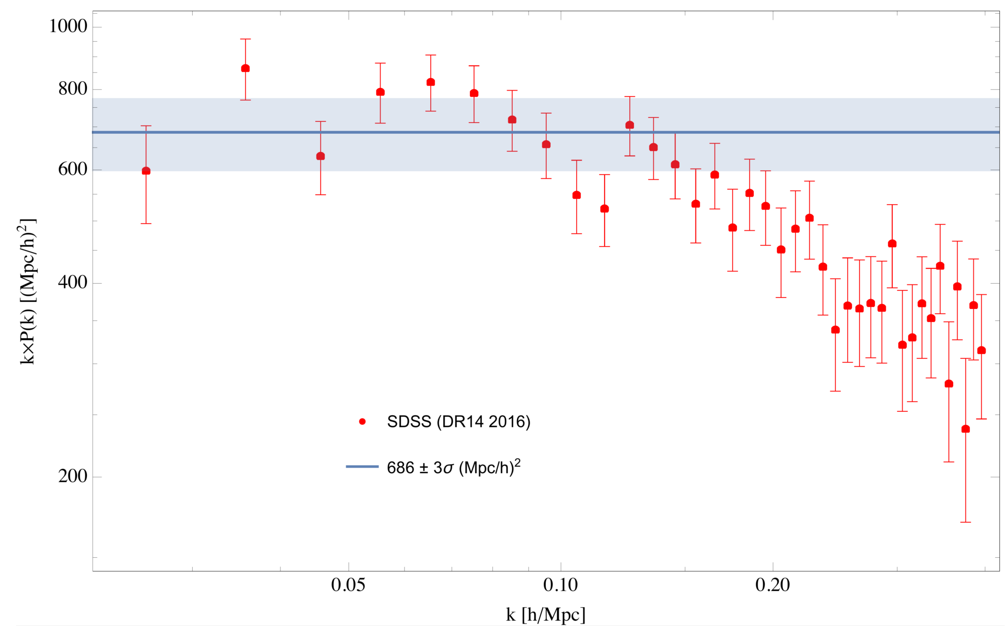
Appendix A). From the observational side,
Figure 1 shows recent results of the power spectrum from the 14th data release (DR14) of the Sloan Digital Sky Survey (SDSS), a galaxy survey which charted over 1.5 million galaxies, covering over one-third of the celestial sphere [
70], with separations roughly from
(
) to
(
). Notice as
k decreases (
r increases), the data appears to approach a constant on the
vs.
k plot, which agrees with an
scaling law
One then obtains a value of
, which parameterizes the amplitude of the galaxy power spectrum. In particular, focusing on the linear scaling regime
50 Mpc (
k ≲ 0.15
h Mpc
−1), all of the corresponding 13–15 data points lie within a 3
σ (∼15%) variance of
. On the other hand, as expected, for separation distances smaller than 50 Mpc (
k ≳ 0.17
h Mpc
−1), the spectrum deviates from the
s = 1 scaling law, giving rise to a transient behavior into the nonlinear regime. In addition, rough oscillations from BAOs can also be observed about the average value given by
a0.
One can further extend the above analysis by doing a phenomenological fit over the linear regime with two parameters, and s, using again the scale-invariant ansatz . Such fit gives , i.e., about around the predicted value, and . This is a decent expectation given a first order prediction, neglecting BAOs and other dynamical effects superimposed on the linear scaling. Further analysis by applying the fit over the full range of observational data () gives , i.e., about of the predicted value, and . The larger discrepancy in s is also expected, given that the nonlinear regime is now included in the fit. Nevertheless, it is still overall consistent with an trend, satisfying the general trend created and set by the gravitational correlations. To even more accurately extrapolate the results to the nonlinear regime (), the full nonlinear dynamics has to be addressed and solved. In fact, we will see that the nonlinear solutions can be extrapolated to even larger scales () into a radiation dominated era of the Universe. This will be the topic of the next section.
It should be noted here that the amplitude
, just like the scaling dimension
or
s, is in principle calculable from the lattice treatment of quantum gravity, as discussed for example in [
16] and references therein. Nevertheless, unlike the universal, scheme-independent, scaling dimension
s,
represents a non-universal quantity, and will therefore depend to some extend on the specific way the ultraviolet cutoff is implemented in the quantum theory. This fact is already well known from other lattice gauge theories such as lattice QCD. Therefore it seems more appropriate here to take this non-universal amplitude
as an adjustable parameter, to be fitted and constrained by astrophysical observational data. Nevertheless, quantum gravity provides a direct prediction for the general
scaling of galaxy correlations.
Notice that since galaxy scales from the SDSS survey are of the order
, which is at least one to two orders of magnitude below
, the RG running of Newton’s
G as governed by Equation (
4) is highly suppressed, and Newton’s constant can be treated as a constant. Later on we will explore these additional effects as we turn to fluctuations on even larger scales in the next section.
4. Matter Power Spectrum in the Small- Regime
It is possible to extrapolate the quantum gravity predictions in the linear regime of galaxies to both larger and smaller
k via a solution of the appropriate nonlinear evolution equations. The calculation is one that is rather complex algebraically and is often done via numerical programs such as CAMB. A semi-analytical treatment can be found in [
67], which was adopted in our previous paper, and which will be used here as well. More details of the calculation can be found throughout our previous work [
15], and we will simply outline the key steps in this section, as well as present the latest observational results.
Already mentioned is the challenge of extending to smaller, nonlinear, scales (
). But a second challenge is to extend to larger distances (
). Larger distances in the sky correspond to earlier epochs of the Universe, which eventually transits from a matter dominated one to a radiation dominated one, which takes place around
[
18]. For such distances (
) which correspond to a Universe that is constitute predominately out of radiation, it will be difficult to find fully formed galaxies. Therefore the main source of observational data that involve such large separations comes from the observed cosmic microwave background (CMB).
However, the map of the CMB represents fluctuations in temperature, which are essentially fluctuations in radiation, not matter, density. The quantum gravity prediction of for the scaling of curvature fluctuations is in principle valid for all scales of separations (up to , or ). However, whereas the scalar curvature correlation is easily related to the matter density correlation using the trace of the Einstein field equations in (where the Universe is matter dominated), it is not easy to relate to a radiation correlation for (where the Universe starts to become radiation dominated), since the trace of the energy-momentum tensor for radiation is zero. In this case the full Einstein field equations, not just their trace, is needed.
Both challenges can be circumvented via existing numerical calculations of the nonlinear cosmic evolution equations. For minimal confusion, we will strictly adhere to the notation in [
67] for the derivations and expressions for
, and later
’s, unless otherwise stated. Their general solution for
is given by the form
where
, a prefactor of cosmological parameters. An initial condition is imposed on the factor
, and the rest is the so-called transfer function
, a well-known result from standard cosmology literature [
71]. A semi-analytical formula for
is given by
in [
67], with
, and will be used here for simplicity. The remaining initial condition function
is usually parameterized in the form of a scale-invariant spectrum [
72,
73,
74]
which then forms the only ungoverned part of the power spectrum
. In other words, the full power spectrum, over a full scale of
k, is now parameterized by only two theoretical parameters,
and
. The rest is then fully governed by classical physics and measured cosmological parameters. The quantity
is sometimes referred to as the “pivot scale”, and here is simply a reference scale, conventionally taken to be
.
One can now normalize the spectrum from the galaxy regime (see [
15] for details), and then the full power spectrum up to
Mpc (
) is fully determined.
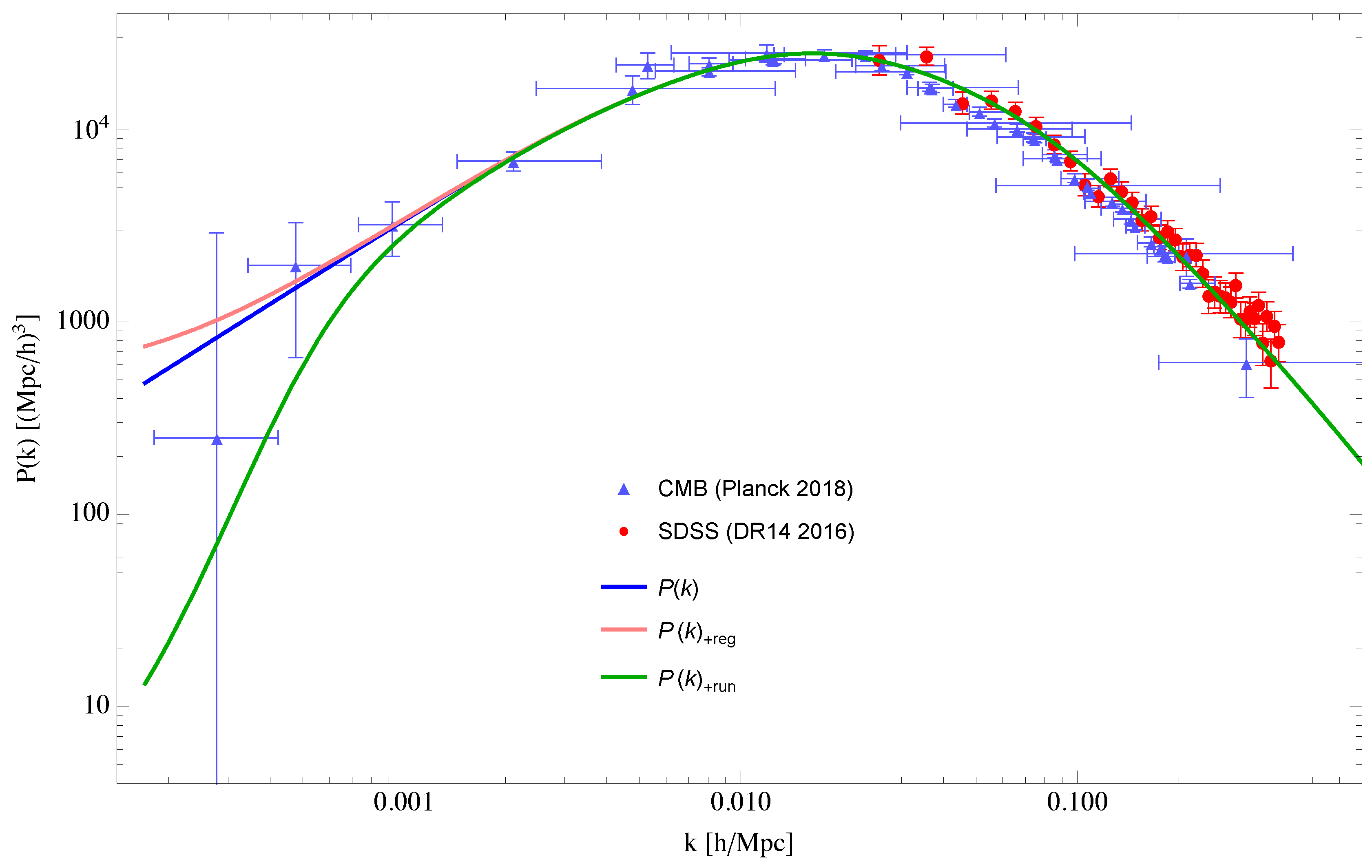
Figure 2 shows this prediction by the middle blue curve with the CMB data from the Planck satellite data (2018) [
18], combined with the earlier galaxy data from SDSS (DR 14). As one can see, the middle blue curve is in good agreement with all the current CMB and Galaxy data points. This shows that applying quantum gravity results, together with standard cosmology derived from the Boltzmann transport equations and general relativity, provides a complete derivation of the power spectrum
.
Now, at scales above
Mpc (or
k below
), additional quantum effects are expected to be significant in the quantum theory of gravity. These effects can form potentially testable predictions for this picture which deviate from the current classical predictions. Indeed, at small k, two additional genuinely quantum effects becomes important. Firstly, similar to QCD, an infrared (IR) regulator must be included to regulate expressions near vanishing
k. This is implemented, in close analogy to QCD, by promoting in various expressions
where the scale
. Secondly, the effects of renormalization group (RG) running of coupling constants will become significant at small
k, which involves promoting Newton’s constant
G to
Both effects are plotted in
Figure 2, with the top pink curve showing the first effect of an IR regulator, and the bottom green curve incorporating both effects together. Note that the combined effect is a dip below the classical (blue curve) results at scales of around
. The deviation in these curves can potentially form a testable prediction of the quantum gravity picture, with increasingly precise results expected in the near future.
It is worth comparing the above results to the inflation-motivated picture. In essence, the inflation picture postulates a scalar field that is dominant in the early Universe (with some power-law potential), whose quantum fluctuations sets the scale of the fluctuations of the (Newtonian) gravitational potential
. The inflaton field then needs to be “turned-off”, after some
number of
e-foldings, and the spectrum for gravity
continues to govern the spectrum for matter, resulting in the observed matter spectrum today. It should be noted that the success of inflation has been largely attributed to its ability in explaining this power spectrum. Prior to inflation, the origin of this spectrum has long been a mystery. At the time, models such as a fractal Universe [
1] provided the best motivation for the Harrison-Zel’dovich spectrum of
in the galaxy regime. Nevertheless, the origin of this fractal behavior remained a mystery. With the invention of inflation, finally comes a quantum theory that is able to set the initial scale, and provides an explanation with a “primordial spectrum” that leads to
having a value
for basic scalar models assuming
e-foldings. This prediction, which provided the first explanation for the shape of the power spectrum, has thus been presented as a triumph of inflation [
69,
75].
Here we have presented an alternate picture, whereby treating the gravitational field quantum mechanically one is able to extract the gravitational scalar curvature spectrum , which then directly governs the power spectrum for matter . The scaling of the gravitational spectrum is, whether evaluated numerically or estimated analytically, fully calculable from first principles of quantum field theory. Furthermore, the relation from the curvature spectrum to the matter spectrum is also in principle unambiguous, as presented in this work.
It is interesting to note that the scalar spectral index
can also be extracted from this picture, which leads to some interesting comparison. The scaling indices for the gravitational curvature spectrum
and
gives roughly
[
15]. There are however a number of uncertainties through this derivation, from the evaluation of the true values of
,
and
s, to normalizing the full spectra. It will require more work in the future to narrow down the exact uncertainties in these various steps. From our first-order calculations, we arrive at a value for
within ∼
of the measured value from Planck [
18] and in spite of these uncertainties, which seems reasonable for a very first attempt.
Despite the crude discrepancy at this stage for , which presumably can be improved with more precise studies, there are a number of advantages for this gravitationally motivated picture, compared to the inflation motivated one. The gravitational scenario does not require the postulate of an undiscovered quantum field and its fluctuations, but simply utilizes the quantum fluctuations of the existing gravitational field, which most current discussions neglect. Secondly, unlike inflation models, the theory of quantum gravity is at least in principle unique. The number of tunable parameters is extremely minimal and, most of them, in principle can be nailed down with further studies.
It should also be pointed out that the far left data point (at
) was released by Planck [
18] only around one week after publication of our previous paper [
15], suggesting a reduction in power on the very low
k, and thus somewhat supporting the quantum gravity prediction. It is obvious that the significant magnitude of the error bars for this last point makes it vastly premature to make any definite conclusions. However, the fact that the data point was published after the publication of the first paper could make it a genuine prediction of quantum gravity, instead of a post-diction, like the rest of the data points. The publication of this new (and previously non-existent) data point suggests the predictability and testability of the quantum gravity picture presented here. It is hoped that this can be done via new astronomical experiments and observations in the near future, which will further improve and narrow down the errors in the small-
k, and which may serve to verify (or falsify) this theory.
As a final note, it should be noted that the inflation picture requires setting the scale of the spectrum with
at small
k’s. It would be difficult for at least basic inflation models to reproduce a dip for
. As a result, with future observational experiments, further narrowing of errors bars in the low-
k regime may be possible to provide a clear distinction between the competing gravitational and inflation picture. More detailed comparisons and computations can be found in the previous paper [
15]. In summary, compared to inflation, the gravitationally motivated picture provides in our view a competing alternative explanation for the power spectrum in terms of both its naturalness and its uniqueness.
6. Constraining the Running of from Cosmology
A similar study can be performed for the magnitude of the RG running of
G, and specifically the key quantum amplitude
. Recall that the running of
G is given by
where
is the currently established laboratory value for Newton’s constant, the quantum amplitude is
, and the nonperturbative gravitational condensate scale is estimated at
Mpc. The value of
is computed from the Regge-Wheeler lattice formulation of quantum gravity [
41,
42,
43]. This is largely in exact analogy, both in concept and in practice (via the lattice), to the evaluation of the
function in QCD. The latter represents a quantity that has been extensively tested in collider experiments, and is by now in extremely good agreement with accelerator experiments. At this stage, unlike
from QCD, the same level of precision has not yet been achieved for
, and it seems possible at this stage, given various numerical uncertainties inherent in the calculation of
, to have deviations that could modify it by up to an order of magnitude.
As a result, one can parallel the previous study of
, and utilize cosmological data to provide a best-fit value, and thus a constraint, on the quantum amplitude
. Also, the same type investigation for the variance in
will be done at the end of this section.
Figure 4 shows the best fit to
, which corresponds to roughly
-th, or
, of the original value for
, i.e.,
(in solid purple). The bands above and below the solid purple curve represent a further factor of
and 2 respectively.
Note that the middle solid (purple) curve with
modified to
can also be mimicked by instead tuning
to ∼
Mpc (
Mpc) and keeping the lattice value for the amplitude at
. The initial association of
Mpc is theoretically motivated by connecting the curvature vacuum condensate scale in the theory,
, to the nonperturbative correlation length
[
44,
45], and again in close analogy to what happens in QCD (the factor of
is often accompanied with
in the equations of motions, such as the classical Friedman equations). It is thus conceivable that the order of estimate
can be varied by a factor up to an order of magnitude. The above analysis shows that, if the lattice value of
is to be taken rigorously, then an increase of ∼
on the vacuum scale
would best fit the data. In essence, the RG running of Newton’s constant
G requires two parameters, the quantum amplitude
and the correlation length
, to fully determine its form. The former is in principle calculable from the lattice, while the latter is best associated with the scale
provided by the theory, which determines the long-distance decay of Euclidean curvature correlation functions at a fixed geodesic distance. Nevertheless, the error bars in the last data point in
Figure 4 are too wide to provide any definite conclusions at this stage. It is conceivable that further satellite experiments might put further constrains on the errors in these points, and thus provide more insight on these fundamental microscopic parameters.
Here we note that it is of some interest to explore analytical (as opposed to numerical) methods related to the running of Newton’s constant
G. One possibility briefly mentioned earlier is the
expansion [
46,
47,
48,
49,
50,
51,
52,
53], which provides an estimate for the scaling exponent
to be between 2 and 4.4, through a one- and two- loop double expansion (in
G and the dimension) respectively, giving additional confidence in the numerically computed value
. Similar estimates for the exponent
are found within a set of truncated RG equations, directly in four dimensions [
58,
59,
60,
61,
62,
63,
64,
65,
66].
Another recently explored idea is a nonperturbative approach via a mean field approximation, which in this context is essentially the Hartree-Fock (HF) self-consistent method applied to quantum gravity [
19], used here for the running of Newton’s constant
G. One finds the following expression for the running of
G,
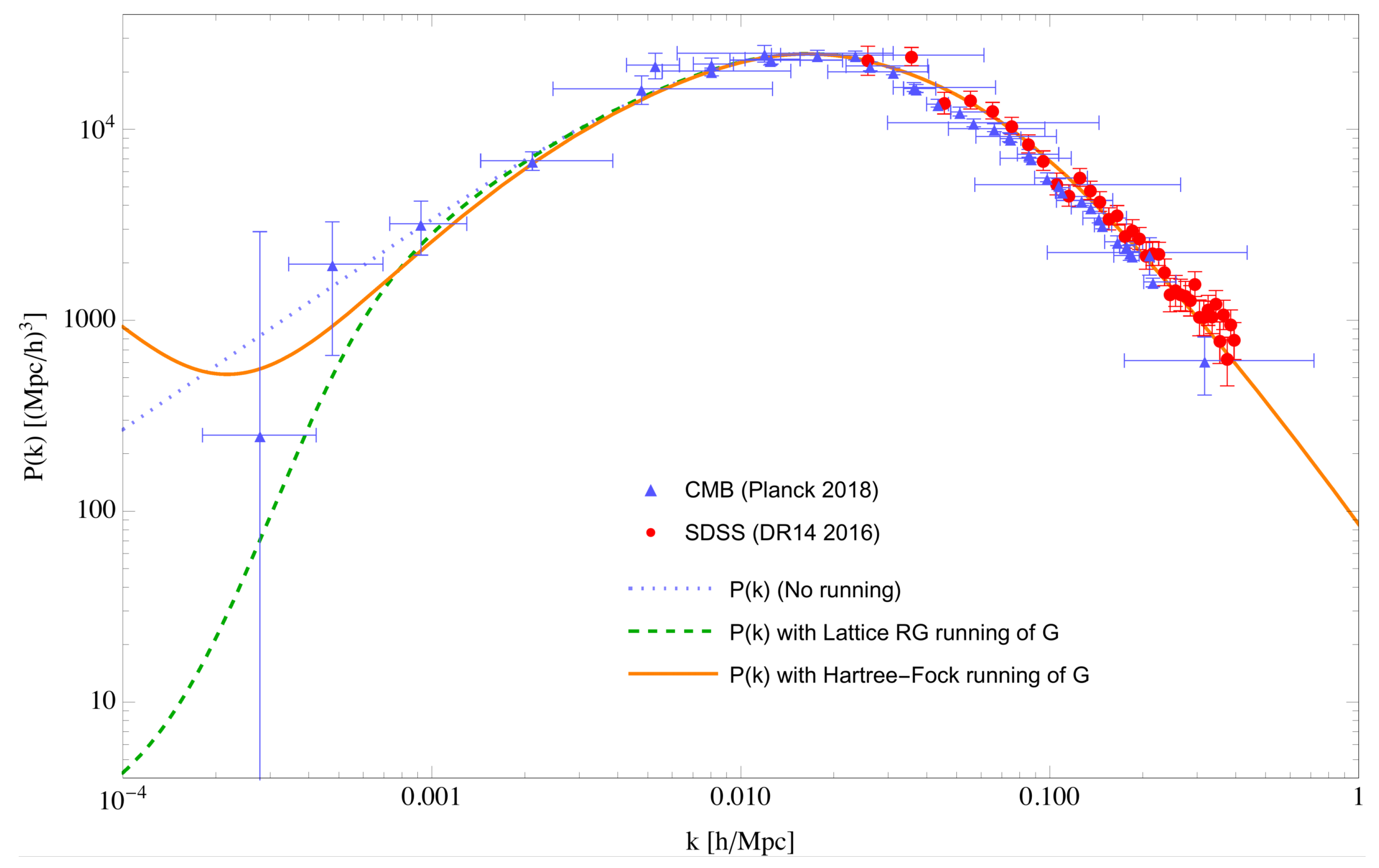
The result of this exercise is shown in
Figure 5. The middle solid orange curve shows the Hartree-Fock expression for the running of Newton’s constant
G, while the bottom dashed green curve and the top blue dotted curve show the original lattice running of Newton’s constant
G (with original lattice coefficient
), as well as no running respectively for reference. It seems that the Hartree-Fock running of
G is in good consistency with the lattice expression, except for the eventual unwieldly upturn beyond
. However, this upturn is most likely an artifact from the Hartree-Fock expression being just a first-order analytical approximation after all (it is well known that the Hartree-Fock approximation can be extended to higher order, by including increasingly complex higher loop diagrams, with dressed propagators and vertices still determined self-consistently by a truncated version of the Schwinger-Dyson equations). Nevertheless, the Hartree-Fock approximation shows good consistency with both the latest available observational data sets, as well as with the lattice results. The fact that it exhibits a gentler dip at small k perhaps also provides support for the reduced lattice running coefficient of
from
Figure 4.
7. Angular CMB Temperature Power Spectrum
The most accurate recent measurements of the CMB are actually represented by the angular temperature power spectrum, represented by a set of angular Fourier coefficients denoted by
. It is therefore useful to translate the quantum gravity prediction to the angular temperature spectrum represented by the
’s. The angular temperature spectrum
coefficients relate to a two-point correlation function of the temperature, when expanded in terms of spherical harmonics labelled by
l and
m. The
coefficients themselves are defined as
where
are two different directions in the sky, and
the Legendre polynomials. Here we avoid the usual common notation, “
”, for the Legendre polynomials, in order to avoid unnecessary confusion with the various power spectra. Following [
67], fluctuations in the CMB temperature
can be expanded in plane waves,
where
K (the average CMB temperature measured today),
the time of recombination, and
form factors given by
The
B and
E functions describe suitable decompositions of the metric perturbations, and
is the velocity potential for the CMB photons. These form factors simplify for certain gauge choices. In the synchronous gauge,
, whereas in the Newtonian gauge
and
, which then gives
The functions
and
, as well as the scale factor
and
, can all be obtained as solutions of the classical Friedmann equations combined with the Boltzmann transport equations, as is done in standard cosmology, which will then in principle lead to unambiguous predictions for the
’s. Note that
and
are referred to as “
” and “
” respectively in [
67]. Here we will use the former in order to avoid confusion with the expression for the running of Newton’s constant
, as it will be implemented below. We also make the usual approximation of a sharp transition at
during recombination, which is quite acceptable since we are primarily interested in the general trend, and not exceedingly precise features, of the spectrum at this stage.
Perturbations in the above form factors are fully governed by the classical Friedmann and Boltzmann transport equations. These lead to standard solutions in terms of transfer functions
,
and
, given by
where
,
,
Mpc,
Mpc,
Mpc,
Mpc, and
. It is noteworthy at this stage that all three transfer functions are completely determined again by (well measured) cosmological parameters. So the only remaining ingredient to fully determine the
coefficient is an initial spectrum
, which is usually parameterized by an amplitude
N and spectral index
,
Here the reference “pivot scale” is usually taken to be
by convention. As a consequence, once the primary function
is somehow determined, classical cosmology then fully determines the form of the
spectral coefficients. It is therefore possible to write the
’s fully, and explicitly, in terms of the primary function
. After expanding the original plane wave factor in a complete set of spherical Harmonics and spherical Bessel functions, one obtains
Here
, and we have factored out the function
explicitly
and
. Recall that, since the matter power spectrum is given by
we can use
to obtain a direct relation between the
’s and
,
where
q and
k are related by
, and the scale factor “today”
can be taken to be 1.
The quantum theory of gravity, as outlined in the earlier sections, predicts the form of the full matter power spectrum function
. Using Equation (
39), one can therefore translate the quantum gravity prediction on
to the angular coefficients
’s.
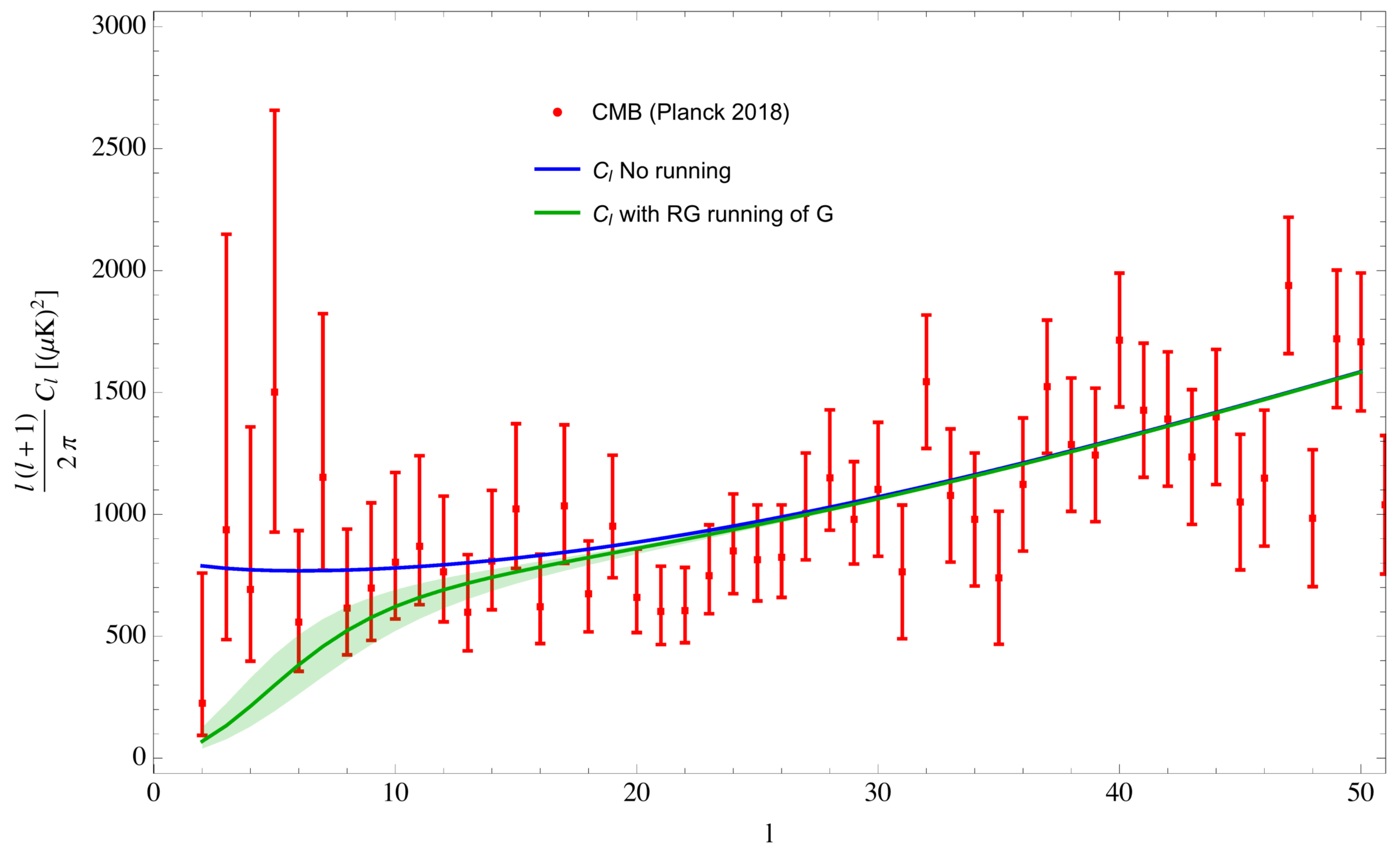
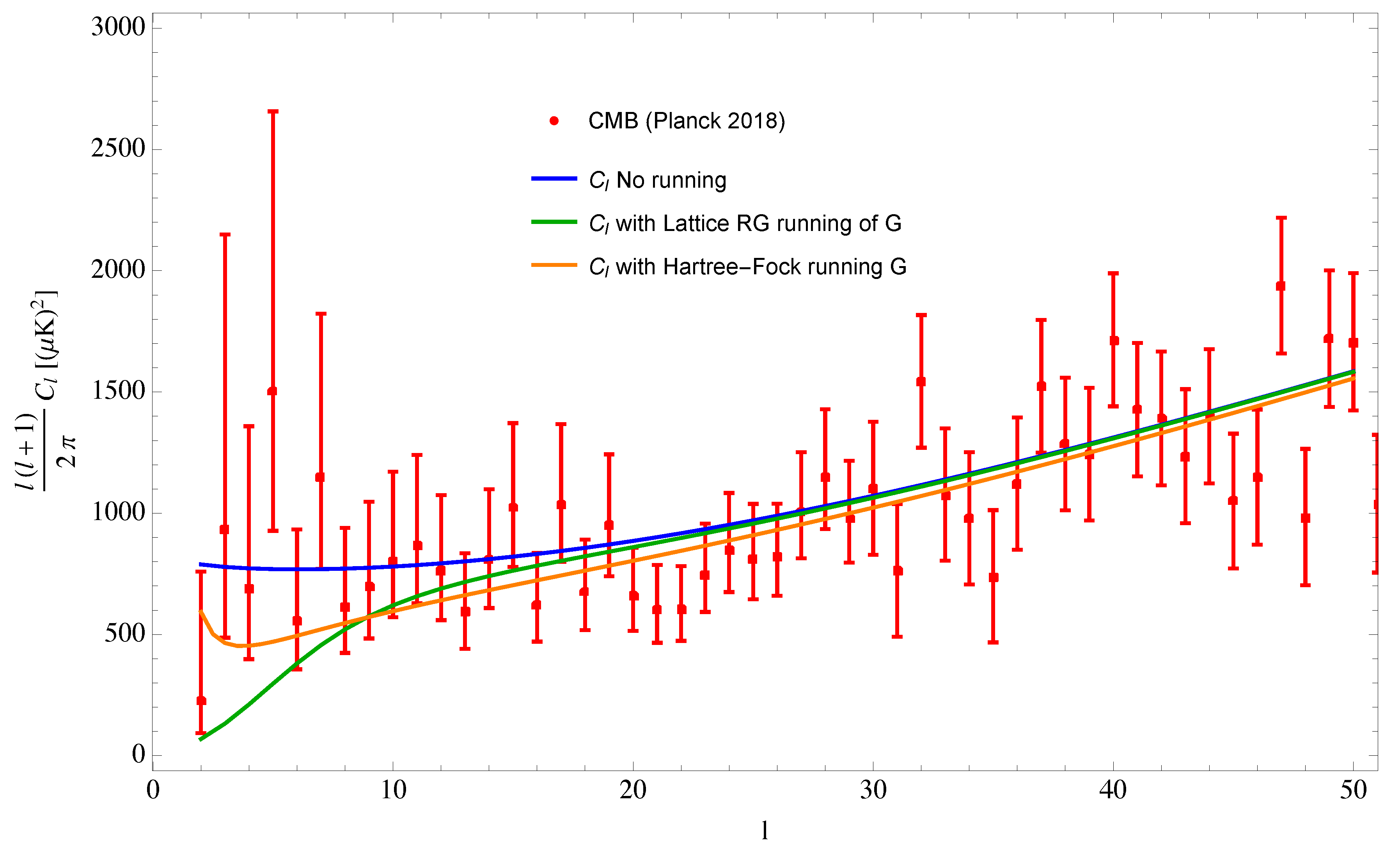
Figure 6 shows a plot of the ensuing result, represented by the top blue curve, for
to
. One can see that the theoretical prediction (obtained here by numerical integration) is in generally rather good agreement with most of the observational data.
Again, it should be emphasized here, again, that reproducing the full expression for the ’s does not require the inclusion of a scalar field anywhere. Instead, the spectrum for gravitational fluctuations is used to set the scaling in a particular regime, which is chosen to be the galaxy regime for its most direct connection, and the rest is then fully governed by classical general relativity and standard kinetic theory. Another way of expressing this result is that the entire expression for the ’s, or for , except for the spectral index and the amplitude N, is fully governed by classical general relativity and kinetic theory (and by finely measured cosmological parameters such as , , , etc. …). That is, and N are the only two remaining theoretically undetermined quantities in this framework. Whereas inflation provides one perspective on how these two parameters can be derived, quantum gravity provides in our view an equally well-motivated alternative.
However, as before, additional quantum gravity effects are expected to manifest themselves at very large distances comparable to
. In angular space, this corresponds to the widest angles, or very low-
l regime. In this context one can then investigate how the IR regularization and the RG running of Newton’s constant
G affects the standard prediction, thus providing potentially testable predictions and alternatives, to distinguish between this quantum gravity fluctuation picture and the inflation one. In the case of the matter power spectrum
, the RG running of Newton’s constant
G was implemented by modifying
where
is the Newton’s gravitational constant measured in the laboratory or on solar system scales. In the angular spectrum coefficients
, this will introduce an extra factor of
in the integrand. The resulting modification is shown by the lower green curve in
Figure 6. As for the case of
, the RG running of Newton’s constant
G causes a significant drop in the magnitude of the
’s at large distance scales (low
l). The green bands around the curve with the RG running of Newton’s constant
G shows the effects of varying by factor of 2 the quantum running amplitude
.
Note that in particular the last point at , which corresponds to measuring the CMB on the largest scales on the sky, is significantly below the classical prediction, and has represented a well-known anomaly for quite some time. Although that last point is plagued with large uncertainties due to cosmic variance - the lack of independent samples on this scale from our sky - many do agree that the error bars as shown already account for our best assessments of the associated variances. If these judgements are believable, then the classical prediction seems just marginally consistent with the allowed uncertainties. If the matter power spectrum indeed originates from inflation, then there are currently no widely agreed solutions that can reasonably explain the sudden drop in power at the extreme low l’s. This is a general consequence of inflation, providing a scale-invariant normalization at very large scales.
Quantum gravity, however, tells us that the effects from a running Newton’s constant
G must be included, whether by an expression calculated from the lattice approach as represented by the green curve above, or by one calculated via the Hartree-Fock approximation.
Figure 7 shows a comparison between them.
So it seems that for distance scales roughly , both quantum gravity and inflation produce a spectrum that agrees rather well with observations. Although one can argue the gravity induced perspective is more natural to the principle of Ockham’s Razor, being able to explain the same physical phenomena without the need of a new field, the question of which picture is more desirable remains largely a philosophical one. However, for distance scales roughly (i.e., small k or small l), both the observed matter power spectrum and the corresponding observed angular power spectrum seem to hint towards the quantum gravity picture. Of course, ultimately, much more precise data will be needed to conclude this decisively. Nevertheless, the current context presents an intriguing possibility for a new explanation for the nature of correlations and for the origin of cosmic fluctuations, and also beyond that an interesting testing ground for quantum gravity.
It is of some interest here to compare the running of Newton’s constant
G obtained from the lattice to the analytical result of the Hartree-Fock approximation. Using the Hartree-Fock expression Equation (
27), the corresponding result is displayed by the orange curve in
Figure 7. One notes that, similarly to
, the Hartree-Fock expression analogously (i) predicts a smaller power in the low-
l’s (
), (ii) has a less dramatic dip compared to the lattice running at the very large scales (
), and finally (iii) predicts a somewhat unwieldly upward turn at the extreme large scales (
). As is the case of the matter power spectrum
, some of these features, especially the unwieldy upturn at extremely large scales, may be an artifact from the fact that Hartree-Fock is essentially a mean-field type approximation. Nevertheless, while the lattice prediction may be more trust-worthy due to it being an exact, numerical evaluation of the path integral, the Hartree-Fock expression provides a good independent consistency check for this picture.
Finally, it is possible to investigate the effect of varying the lattice quantum amplitude
appearing in the running of
G, as in Equations (
4) and (
6). From the investigation of
, the value of
that best fits the large scale data at small
k is
.
Figure 8 plots the effect of this modification. As before, this choice seems to fit rather well with most of the data in the low-
l regime. Nevertheless it should be noted that this modification can also be mimicked by modifying the correlation length
Mpc to
Mpc, or by any combined adjustments of the two parameters
and
.
Although at first sight it may seem impossible to eventually distinguish the difference between the classical and quantum picture by the still highly uncertain data, it may not be so with better telescopes in the near future.
Table 1 shows the percentage difference between the classical prediction, and one with the RG running of Newton’s constant
G included, in accordance with Equation (
6), with the choice
.
From
Table 1, one can see a
difference in the
for
, which future experiments may be able to distinguish. However, too much emphasis should not be put in the extreme low-
l points due to statistical limitations arising from cosmic variance, which under reasonable assumptions (mainly Gaussianity) is expected to grow rapidly as
l decreases, by
[
67]. Nevertheless, focusing on the
to
points, the narrowing of errors needed to distinguish between the classical and the quantum predictions may very much be achievable. Thus, for example, for
, the percentage difference between the predictions is
. In comparison, the current errors on the Planck data for the
value is
. For
, the current uncertainties in the Planck data is
, whereas the difference between the classical and quantum prediction is only
, which may be more difficult to resolve with future satellite experiments. Nonetheless, the magnitude of the errors in the CMB observational data may initially seem unpromising to make any claims, this table shows there may still be hope in distinguishing the various theoretical predictions. Within the
to
points range, the improvements in technology needed to improve the measurements and support the validity of the gravitational fluctuation picture may actually be within reach in the next decades, which provides an exciting prospect for the future.
In conclusion, in this section we showed how the quantum gravitation prediction for unambiguously translates to a prediction for the ’s - which is essentially related to the former via a spherical Bessel transform, weighted by some suitable combination of transfer functions. The transfer functions in turn are ultimately just solutions to the classical Friedmann equations and associated Boltzmann transport equations which, apart from the measured values of standard cosmological parameters such as , , etc., require no further theoretical input. As a result, we were able to show how the quantum gravity prediction for the matter power spectrum directly and unambiguously translates to the angular coefficients . It can be seen that the prediction is rather consistent with current cosmological data.
We also discussed several theoretical parameters, which in this picture potentially have some variance and related uncertainties. The first two key parameters in the quantum gravity motivated picture are the universal scaling exponent
, and the fundamental vacuum condensate correlation length
. A third additional parameter here is the quantum amplitude
, which governs the amplitude of quantum correction in the RG running of Newton’s constant
G as given in Equations (
4) and (
6). Of the three parameters, as shown above in
Section 5,
is pretty much highly constrained (both theoretically and observationally) around
. The value of this last parameter should also be the most trustworthy of the three, since, as a universal scaling exponent, it is expected to be entirely independent of schemes and regularization. On the other hand, the values of
and
are somewhat less definite. Here the nonperturbative length scale
is quite analogous (via the observed scaled cosmological constant
), to the vacuum condensate scale in QCD
, or to the scaling violation parameter
. Which implies that it’s absolute value in physical units is not determined theoretically, and can ultimately only be fixed by experiment. Current cosmological data seem to suggest the best - and most consistent - estimate for
is roughly
Mpc, whereas for the quantum amplitude
, or some degenerate combination between the two (as discussed earlier). Finally, we explicitly listed the percentage differences between the classical prediction and the quantum one implemented with an RG running of Newton’s
G, which should provide a useful guide as to how improved observational data must trend in order to support the picture advocated here. Although such precision has not been achieved yet, it should hopefully be attainable in the near future, and thus provide an additional significant test for the quantum gravity picture.
Nevertheless, with these flexibilities in mind, the quantum gravity picture outlined here provides a radically different perspective to the origin of matter and radiation fluctuations, compared, for example, to inflation. In addition, the inflation picture normalizes the spectrum at large scales (i.e., small-k), so that for the ’s it predicts a flat scale-invariant plateau for small-l’s. If the last point of is to be taken seriously, despite the flexibility inherent in various inflation models, it would be difficult to account naturally for the reduction in power on the very largest scales. In contrast, the demand of a renormalization group running Newton’s constant in the quantum gravity picture appears to explain the dip quite naturally. Of course, due to the large uncertainties in the data at small l’s, significant improvements on the errors needs to be made before definite conclusions can be drawn.
8. Conclusions
In this paper, we have revisited the derivation of the galaxy and cosmological matter power spectrum that is purely gravitational in origin, which is to our knowledge is the first of its kind without invoking the mechanism of inflation. We provided updated observational data, including revised experimental errors, and outlined an elementary study of the uncertainties involved for the theoretical parameters in this picture, including the universal scaling exponent , the quantum amplitude and the nonperturbative scale . We also presented the Hartree-Fock results for the running of Newton’s constant G, in the form of an analytical approximation, for a useful comparison with the Regge-Wheeler lattice result. We then extended our predictions to the angular temperature power spectrum and repeated and extended the uncertainty analysis. In both cases, we showed good general consistency of this purely gravitationally motivated picture with current observational data, and pointed out a significant deviation from the inflation motivated predictions in the large distance scale regime. Although experimental errors and cosmic variance are large in this regime, these results provide a potentially exciting area that can verify, or falsify, the various pictures.
To reiterate, the primary benefit of the quantum gravity explanation over inflation is the non-necessity for additional and untested physics ingredients, other than standard Einstein’s gravity and accepted modern quantum field theory methods. The basis of the methods begins with the path integral formulation of gravity [
20,
21] which, unlike inflation, provides a very constrained theoretical framework. Also, given the well-known fact that the theory is not perturbatively renormalizable, standard nonperturbative methods and approaches must be used. While a lot of the results used here are derived from the lattice numerical treatment, additional confirmations via analytical methods are also briefly discussed, including the 2+
and the Hartree-Fock approximation. The general consistencies of these numerical and analytical methods gives confidence to the results. The lattice treatment in particular has a long history of high precision success in other fields, from QCD to condensed matter and statistical systems, and thus provides us with particularly trustworthy results.
On the other hand, for inflation, a new, minimum of one, inflaton field, usually scalar in nature, must be invoked. The details of the particular theory are also highly flexible, leading to a myriad of models, see for example [
76] and references therein. In addition, recent studies have shown that a majority of single-field inflation models have either been ruled out or highly constrained. The amount of flexibility for inflation has thus led many to question the predictability and ultimate naturalness of such scalar-field based solutions [
77,
78,
79,
80,
81,
82]. Although the original model of inflation was invented to explain the flatness and horizon problem, it has been convincingly argued that it is not a necessary ingredient to do so [
83,
84,
85,
86,
87,
88,
89,
90,
91,
92,
93,
94,
95]. We have argued therefore that the gravitational picture provides a more concrete and natural explanation to the origin and distribution of cosmological matter fluctuations.
Finally, we have pointed out that the gravitational fluctuation picture also provides a clear set of predictions that diverge from scalar field induced predictions on very large scales. As advanced satellite experiments are continuously being conducted, and increasingly accurate measurements are becoming available, the predictions originating in quantum gravity outlined in the previous section could be verified or disproved in the near future.
We should add that it is certainly possible for our picture of gravitational fluctuations to even coexists with inflation, with both effects providing significant contributions to power spectra. Nevertheless, we do not explore this idea in depth here, as the primary aim of this paper is to show that the same power spectra can be reproduced purely from macroscopic quantum fluctuations of gravity, independent of any inflation mechanism, making use of well-accepted and tested methods for dealing with perturbatively nonrenormalizable theories. Still, this could be a potential avenue for future explorations.
In addition to the results presented here, there are also a number of exciting future directions which seem meaningful to explore. For example, the quantum gravity-based explanation is most certainly not Gaussian, due to the presence of non-trivial anomalous scaling dimensions [
16] which affect all gravitational
n-point functions, although they may seem to be Gaussian in certain regimes. While the corresponding predictions for the two-point functions, or power spectra, are similar to those motivated by inflation, a divergence will definitely be expected on higher order
n-point functions, commonly known as bispectra and trispectra in the cosmology context. For example, the two-point function scalar curvature result of Equation (
17), derived from quantum gravity, will also determine the form of the connected reduced three-point function, or bispectrum, for large scale scalar curvature correlations [
16]
with constant amplitude
, and relative geodesic distances
in coordinate space. It is easy to see that this last correlation leads to a Fourier transform in momentum- or wavenumber-space of the form
where
are the three momenta conjugate to
, the scale
, and
is Euler’s constant. The overall multiplicative constant in Equation (
42) is
, with the expectation that
if the curvature two point function of Equation (
17) is normalized to unity (see further discussion below). One can then follow the same line of argument given in
Section 3 to relate this to measured quantities from the CMB. Here we outline the main points of the argument. Firstly, the Einstein’s field equations of Equation (
14) allow this bispectrum for curvature to directly translate to the bispectrum for matter
. Secondly, the transfer function, responsible for turning the two-point spectrum from ∼
to ∼
k when connecting the late-time galaxy regime to the early-time CMB regime, essentially supplies an extra factor of
k for each fluctuating field. This then leads to the result
Nevertheless, most CMB bispectrum measurements are presented nowadays in terms of the Bardeen field
, which roughly relates (as it describes a specific metric component) to the curvature by
in the weak field limit. This supplies an additional factor of
for each field, giving the following explicit prediction for the bispectrum of the
field
Here the quantity
here represents an overall dimensionless amplitude for the expected non-Gaussian effects.
However, these non-Gaussian amplitudes are expected to be rather small, with suppressions by factors of
[
16]. This follows simply from the fact that in real space one has for the semiclassical curvature two-point function
, whereas for the scalar curvature three-point function
, and also
etc., where
r here represents the relevant and appropriate combination of relative distances for each reduced curvature
n-point function. As a consequence, in Equation (
44)
where the remaining amplitude
inherits additional transfer function parameters from
and
as in Equation (
22), so that here
. More detailed analyses on this issue, and on the magnitude of these bispectra, shall be left for future work. Nevertheless, it should be clear at this point that analogous results, as hinted above, can also be derived for various four-point functions. We note here that the relevance and measurements of such nontrivial (non-Gaussian) three- and four-point matter density correlation functions in observational cosmology were already discussed in detail some time ago by Peebles in [
2]. The results presented here imply that further observational constraints on these higher order
n-point functions could potentially provide additional tests on the vacuum condensate picture for quantum gravity as outlined in [
16], and more specifically the implications of a non-trivial gravitational scaling dimensions scenario as described previously.
In addition, it is clear that the gravitational fluctuation-based explanation presented here should also give rise to nontrivial tensor perturbations, of magnitude comparable to the scalar one. This could lead to new insights on the corresponding tensor-to-scalar ratio parameter
r [
75], and to a number of potentially interesting and testable consequences to be explored. Here we note that tensor perturbation require at first the knowledge of the semiclassical Ricci tensor (as opposed to the scalar curvature) correlation functions,
with polarization tensor
P and relative geodesic distance
in coordinate space. These correlations have not been measured yet on the lattice, but should be calculable in the near future. Nevertheless, based on the known scaling dimension for the scalar curvature, one would expect here the same result for the operator
, namely
, as in Equations (
3) and (
41) for the scalar curvature
R case. In turn, these curvature correlations functions can then be related to suitable matter and radiation sources, via the quantum equations of motion
with the (trace reversed)
here representing either matter or radiation contributions, and thus in complete analogy to what was used earlier in Equation (
14), and following, for the scalar (trace) case. Since the scalar curvature correlation function of Equation (
3) involves traces of the Ricci tensor (here we make use of the weak field limit)
versus say the tensor correlation
, one would expect, based just on Lorentz symmetry, for the ratio of tensor over scalar correlation amplitudes
. The translation of these simple results into measurable cosmological predictions is of course a lot more complicated.
In conclusion, the ability to reproduce the cosmological matter power spectrum has long been considered one of the“major successes” for inflation-inspired models. Although within our preliminary study, further limited by the accuracy of present observational data, it is not yet possible to clearly prove or disprove either idea, the possibility of an alternative explanation without invoking the machinery of inflation suggests that the power spectrum may not be a direct consequence nor a solid confirmation of inflation, as some literature may suggest. By exploring in more detail the relationship between gravity and cosmological matter and radiation, together with the influx of new and increasingly accurate observational data, one can hope that this hypothesis can be subjected to further stringent physical tests in the near future.


