On the Structure of the Vacuum in Quantum Gravity: A View from the Asymptotic Safety Scenario

Abstract

Although the Asymptotic Safety scenario is one of the most promising approaches to quantum gravity, little attention has been devoted to the issue of the vacuum state. Higher derivative operators often appear on the ultraviolet critical surface around the non-Gaussian fixed point generating additional degrees of freedom which can render the standard vacuum unstable. When this happens, translation and rotational symmetries can be spontaneously broken and a new set of symmetries can show up at the level of the effective action. In this work, it will be argued that a “kinetic condensate” characterizes the vacuum state of asymptotically safe quadratic gravity theories. If this scenario is realized in the full theory, the vacuum state of gravity is the gravitational analogous to the Savvidy vacuum in Quantum Chromo-Dynamics (QCD).

1. Introduction

In the Euclidean formulation of quantum gravity, the notion of a classical metric is formally defined by means of an expression of this kind

$$\langle g_{\mu \nu }\rangle =\int D\left[g\right]g_{\mu \nu }{e}^{-S\left[g\right]},$$

(1)

where a suitable regularization prescription has been assumed. From this perspective, one interprets $\langle g_{\mu \nu }\rangle$ as an order parameter like in the theory of magnetic systems. In particular, $\langle g_{\mu \nu }\rangle \ne 0$ signals a spontaneous breaking of the diffeomorphism invariance and only the stability group of $\langle g_{\mu \nu }\rangle$ is unbroken. For instance, if the latter is the Poincaré group, $\langle g_{\mu \nu }\rangle ={\eta }_{\mu \nu }$ is the Minkowski metric. On the contrary, $\langle g_{\mu \nu }\rangle =0$ represents a phase where the diffeomorphism invariance is fully preserved. Clearly, one of the key issues that a satisfactory theory of quantum gravity must address is to explain why gravity is realized in the broken phase as we observe today at low energies.

Very often in Nature, the ground state does not necessarily share the same symmetries of the equations of motion. Well known examples include equilibrium phase transitions, e.g., the case of a liquid-solid transition where the space-translational symmetry is broken, or a paramagnetic-ferromagnetic transition where the spin-rotational symmetry is broken. In all these cases, the original symmetry is not lost but gives rise to the appearance of a regular structure with a specific length scale, as in the Lifshitz tricritical point in condensed matter theory [1,2].

In the case of gravity, the presence of an ordered phase can thus be understood as the emergence of a specific, non-degenerate, four-dimensional metric in some low-energy limit.

The relevant question is to determine which type of field configurations dominate the path-integral. Let us suppose we make use of a saddle-point expansion so that the most important field configurations are approximated by the solutions of the classical field equations

$$\frac{\delta S}{\delta \varphi }=0,$$

(2)

where $S\left[\varphi \right]$ is the action and $\varphi$ is the fundamental field. Although in simple cases Equation (2) admits only one solution (given a set of boundary conditions), for more complicated Lagrangians (with higher-order derivative operators for example), multiple saddle point solutions may show up. The properties of the vacuum are then determined by the symmetries of the saddle point solution, which might display a rather rich phase structure. Spatially inhomogeneous modes contribute to the expectation values $\langle 0\left|\mathcal{O}\right|0\rangle \ne 0$ of any observable that is sensitive to the nonvanishing kinetic energy of the configurations dominating the functional integral. Here, $\mathcal{O}$ is a scalar operator constructed from the fundamental fields; for instance, $\mathcal{O}={\partial }_{\mu }\varphi {\partial }^{\mu }\varphi$ in a scalar model, or $\mathcal{O}=\mathrm{tr}\left(F_{\mu \nu }{F}^{\mu \nu }\right)$ in Yang–Mills theory. Such contributions are sometimes referred to as “kinetic condensates”. They must be distinguished from the more familiar translational invariant “potential condensates” which underlie the conventional Higgs mechanism.

An example of a kinetic condensate is the gluon condensate in Quantum Chromo-Dynamics (QCD). In this case, the classical action functional $\frac{1}{2}\int d^{4}x\mathrm{tr}\left(F_{\mu \nu }{F}^{\mu \nu }\right)$ is minimized by gauge field configurations with $F_{\mu \nu }=0$, but the effective action has its minimum at $F_{\mu \nu }\ne 0$. An early attempt at finding its global minimum is the Savvidy vacuum [3], in the approximation of a covariantly constant color magnetic field. While its action is indeed lower than that of the naive vacuum with $F_{\mu \nu }=0$, it turned out unstable in the infrared (IR), and it has been argued that the true vacuum should be spatially inhomogeneous. The complexity of the QCD vacuum state is reflected by nonperturbative contributions to $\langle 0\left|\mathrm{tr}\left(F_{\mu \nu }{F}^{\mu \nu }\right)\right|0\rangle$ and similar expectation values of more complicated gauge and Lorentz-invariant operators.

In recent years, recent advances in functional renormalization group methods [4] have offered the possibility to investigate the non-perturbative side of gravity in a systematic way [5]. It has been shown that the Einstein–Hilbert Lagrangian

$$S\left[g_{\mu \nu }\right]=-\frac{1}{16\pi G}\int d^{4}x\sqrt{g}R$$

(3)

describes a theory that can be defined in a consistent way around a non-Gaussian ultraviolet fixed point (NGFP) [6,7] where it is predictive and finite. Encouraging indications that the ultraviolet critical manifold is finite-dimensional have appeared [8,9].

Recent works [10,11] have clarified that the presence of higher-derivative operators like $R^2$ or $C^2$ (where $C^2$ is the square of the Weyl tensor) in the ultraviolet critical manifold is unavoidable. Moreover, it turns out that, in the quadratic gravity theory defined by

$$\mathcal{S}=\int d^{4}x\sqrt{-g}\left[\gamma R-\alpha C^{\mu \nu \rho \sigma }{C}_{\mu \nu \rho \sigma }+\beta R^2-2\Lambda \right],$$

(4)

close to the NGFP, the mass $m_2={\left(\frac{\gamma }{2\alpha }\right)}^{1/2}$ of the spin-2 field is imaginary [10,11]. This result is at variance with the well-known picture for which such a theory is asymptotically free and renormalizable. The spectrum of the physical states is plagued by the presence of ghosts [12], although the ghost might be unstable and hence does not appear in the asymptotic spectrum [13].

Although a negative value of the ratio $\gamma /\alpha$ near the NGFP can be an artifact of the truncation, it is possible that the tachyonic character of the elementary excitations near the NGFP is a genuine feature of a quadratic gravity theory in the Asymptotically Safety program. In fact, recent work with a generic $f\left(R\right)$ [14] has shown that the sign of the coupling $\beta$ of the $\sqrt{g}{R}^2$ operator near the NGFP is stable up to the inclusion of $R^{70}$ terms in the Lagrangian. As the dimensionality of the ultraviolet critical manifold is not changed by the inclusion of the $C^2$ term (which turns out to be a relevant one), it is possible that also the value of $\alpha$ is stable against additional truncations.

If this scenario is realized in the full theory, it is important to study its physical implications, although its non-perturbative character poses serious technical difficulties. In fact, a Lorentz-invariant scalar field theory with spatially modulated vacua has also recently been discussed in [15], but no significant progress in gravity has been made in this respect.

A first step in this direction is presented in this work. In particular, a new class of non-trivial “rippled” gravitational instantons that render the (Euclidean) action (4) finite will be discussed. It will be shown that, at least at a semiclassical level, their impact in the path-integral is a much stronger one if compared with the classical perturbative vacuum. We believe that, albeit very preliminary, this is an interesting result because it can be considered as an indication that the true vacuum in an asymptotically safe quadratic gravity is not the perturbative one, but a “kinetic condensate” like in the conformal sector of $R+R^2$ gravity (see [16]).

2. Higher-Derivative Scalar Theory

Before discussing the case of quadratic gravity, it is instructive to illustrate the kinetic condensate model in the simple case of a self-interacting scalar field theory. Let us in particular consider the following Euclidean action

$$S\left[\varphi \right]=\int d^{d}x\left(\frac{1}{2}\varphi \Omega (-\square )\varphi +\frac{\lambda }{4!}{\varphi }^4\right)$$

(5)

with

$$\Omega (-\square )=\square +\frac{{\square }^2}{2M^2}$$

(6)

so that

$$\Omega \left(p^2\right)=-p^2+\frac{{\left(p^2\right)}^2}{2M^2}.$$

(7)

It is convenient to use a variational approach and consider non-constant test functions (or linear combinations) of the class $\varphi \left(x\right)=A{sin}^n(p_{\mu }{x}^{\mu }+\alpha ){cos}^m(p_{\mu }{x}^{\mu }+\beta ),$ where $\alpha$, $\beta$, m, n and A are free parameters to be varied in order to approach the global minimum of the action. However, for our purposes, it is enough to consider a single plane-wave and chooses $\varphi \left(x\right)=Asin(p_{\mu }{x}^{\mu }+\alpha )$. In this case, $\square \varphi \left(x\right)=-p^2\varphi \left(x\right)$ and $\Omega (-\square )\varphi =\Omega \left(p^2\right)\varphi \left(x\right)$, so that

$$S\left[\varphi \right]=\int d^{d}x\left(\frac{A^2}{2}\Omega \left(p^2\right){sin}^2(p_{\mu }{x}^{\mu }+\alpha )+\frac{\lambda }{4!}{A}^4{sin}^4(p_{\mu }{x}^{\mu }+\alpha )\right).$$

(8)

If $p_{\mu }=p{\delta }_{\mu 1}$, we have

$$S\left[\varphi \right]=\mathcal{V}\left(\frac{A^2}{2}\Omega \left(p^2\right){\int }_{-T/2}^{+T/2}d{x}^1{sin}^2(p{x}^1+\alpha )+\frac{\lambda }{4!}{\int }_{-T/2}^{+T/2}d{x}^1{sin}^4(p{x}^1+\alpha )\right),$$

(9)

where $\mathcal{V}=\int d{x}^2...d{x}^d$. Therefore, in the limit of large T, we can write

$$\frac{S\left[\varphi \right]}{T\mathcal{V}}=\frac{1}{4}{A}^2\Omega \left(p^2\right)+\frac{3}{8}\frac{\lambda }{4!}{A}^4.$$

(10)

If we look for a minimum as a function of p, one obtains

$$\frac{d}{d{p}^2}\left[-p^2+\frac{{\left(p^2\right)}^2}{2M^2}\right]=-1+\frac{p^2}{M^2}=0$$

(11)

so that $p_{\mu }{p}^{\mu }=M^2$; therefore, $p_{\mu }=n_{\mu }M$ with $n_{\mu }{n}^{\mu }=1$. Minimizing over A leads instead to $A=\frac{2}{\sqrt{\lambda }}M$ so that the variational solution is

$${\varphi }_{min-var}\left(x\right)=\frac{2}{\sqrt{\lambda }}Msin(M{n}_{\mu }{x}^{\mu }+\alpha )$$

(12)

with $n\in S^{d-1}$ and $\alpha \in [0,2\pi )$. Note the typical non-perturbative structure of the solution: the frequency of the spatial oscillation is determined by the “mass” M while the amplitude of the field is inversely proportional to $\sqrt{\lambda }.$ Moreover, the value of the action is

$$S[\varphi ={\varphi }_{min-var}]=-\frac{M^2}{4\lambda },$$

(13)

which is unbounded below in the limit $\lambda \to 0$. The lesson from this exercise is that the condensate is inaccessible in perturbation theory. Moreover,

$${\left.\frac{1}{Z}\frac{\delta Z}{\delta J}\right|}_{J=0}=\langle \varphi \left(x\right)\rangle \approx \frac{2}{\sqrt{\lambda }}Msin(M{n}_{\mu }{x}^{\mu }+\alpha ),$$

(14)

where, as usual, $Z\left[J\left(x\right)\right]=\int D\left[\varphi \right]e^{-S\left[\varphi \right]+\int d^{d}xJ\left(x\right)\varphi \left(x\right)}$. On the other hand, if $M^2\to -M^2$ in the original Lagrangian, there is no kinetic condensation and $\langle \varphi \left(x\right)\rangle =0$. The sign of the coupling of the higher derivative operator thus separates the symmetric phase from the broken one, where the familiar $O\left(d\right)$ symmetry is dynamically broken.

3. Kinetic Condensate in $\mathbf{R}+{\mathbf{R}}^{\mathbf{2}}$

A kinetic condensate occurs also to “cure” the instability of the conformal factor in quadratic gravity as showed for the first time in [16]. Let us consider the following Euclidean action

$$S\left[g_{\mu \nu }\right]=\int d^{4}x\sqrt{g}\left\{\frac{1}{16\pi G}\left(-R+2\Lambda \right)+\beta R^2\right\}$$

(15)

with positive cosmological constant and assume $\beta >0$. In general, all stationary points satisfy:

$$\frac{1}{16\pi G}\left[G_{\mu \nu }+\Lambda g_{\mu \nu }\right]+\beta \left[-(G_{\mu \nu }+R_{\mu \nu })R+2D_{\mu }{D}_{\nu }R-2g_{\mu \nu }{D}^{2}R\right]=0$$

(16)

with the Einstein tensor $G_{\mu \nu }\equiv R_{\mu \nu }-\frac{1}{2}{g}_{\mu \nu }R$. Clearly, the task of finding the global minimum is rather complicated due to the presence of possible non-homogeneous solutions with $R\ne constant$, which in principle can further lower the value of the action as in the example of the previous section. In order to better illustrate this point, it is convenient to consider the action restricted to conformally flat metrics, so that

$$g_{\mu \nu }={\varphi }^2\left(x\right){\delta }_{\mu \nu }.$$

(17)

Writing $S\left[\varphi \right]=S[g_{\mu \nu }={\varphi }^2{\delta }_{\mu \nu }]$, the action for the conformally reduced theory reads

$$S\left[\varphi \right]=\int d^{4}x\left\{\frac{3}{8\pi G}\varphi \square \varphi +\frac{\Lambda }{8\pi G}{\varphi }^4+36\beta {\left(\frac{\square \varphi }{\varphi }\right)}^2\right\},$$

(18)

where we used that $\sqrt{g}={\varphi }^4$ and $R=-6{\varphi }^{-3}\square \varphi$ with $\square ={\delta }^{\mu \nu }{\partial }_{\mu }{\partial }_{\nu }$ because $g_{\mu \nu }={\varphi }^2{\delta }_{\mu \nu }$. If $\beta =0$, the above functional has the appearance of a scalar ${\varphi }^4$-action with a wrong sign kinetic term. Clearly, $\varphi =0$ is a solution of the equation of motion, and the value of the action is precisely zero in this case, but other non-trivial solutions are clearly possible, although their analytic form is unknown. Using a variational approach, it is in fact possible to show [16] that the absolute minimum (for $\Lambda =0$) is very well approximated by a single nonlinear plane wave of this type

$$d{s}^2=\frac{2}{2+h^2}{\left[1+hcos\left(\sqrt{\frac{\xi }{48\pi (2+h^2)\beta }}{m}_{\mathrm{Pl}}{n}_{\mu }{x}^{\mu }+\alpha \right)\right]}^2{\delta }_{\mu \nu }d{x}^{\mu }d{x}^{\nu }$$

(19)

with $h\approx 0.58$ and $\sqrt{\xi }\approx 0.45$ and $m_{\mathrm{Pl}}\equiv 1/\sqrt{G}$ is the Planck mass and G the laboratory Newton’s constant. It is important to notice that, if one averages over the characteristic oscillations, a flat metric is recovered as

$$\langle d{s}^2\rangle ={\delta }_{\mu \nu }d{x}^{\mu }d{x}^{\nu }$$

(20)

after averaging.

In Equation (19), the frequency of the oscillations increases for decreasing $\beta$. It approaches infinity in the limit of a pure Einstein–Hilbert action, $\beta \to 0$. Moreover, since $h<1$, the conformal factor has no zeros and the metric is everywhere non-degenerate. The flat spacetime emerges as a result of a coarse-graining on scales larger than the Planck length, but, at a fundamental level, the spacetime structure is characterized by a spontaneous breaking of the Lorentz symmetry.

4. Quadratic Gravity

In this section, non-trivial vacuum solutions of the type described in the previous section will be discussed in a Lorentzian framework, for a generic quadratic gravity theory of the type in (4). The field equations in vacuum (we set $\Lambda =0$) read

$$H_{\mu \nu }=(R_{\mu \nu }-\frac{1}{2}R{g}_{\mu \nu })-\frac{2}{m_2^2}({\nabla }^{\rho }{\nabla }^{\sigma }+\frac{1}{2}{R}^{\rho \sigma })C_{\mu \rho \nu \sigma }+\frac{1}{3m_0^2}(R_{\mu \nu }-\frac{1}{4}R{g}_{\mu \nu }+g_{\mu \nu }\square -{\nabla }_{\mu }{\nabla }_{\nu })R=0,$$

(21)

where $m_0={(\gamma /6\beta )}^{1/2}$ and $m_2={(\gamma /2\alpha )}^{1/2}$. In particular, $H_{\mu }^{\mu }=0$ implies $(\square -m_0^2)R=0$ for $\beta \ne 0$. Let us consider static spherically symmetric spacetimes so that

$$d{s}^2=-h\left(r\right)d{t}^2+\frac{d{r}^2}{f\left(r\right)}+r^2\left(d{\theta }^2{sin}^2\theta d{\varphi }^2\right)$$

(22)

and write

$$h\left(r\right)=1+V\left(r\right),f\left(r\right)=1+W\left(r\right).$$

(23)

Let us further assume that $V\ll 1$ and $W\ll 1$. The linearised field equations can be obtained from the trace equation ${H_{\mu }}^{\mu }=0$ and from the combination $H{}_i^i-H_0^0=0$. One then finds [17]

$$\begin{array}{c}\left({\nabla }^2-m_0^2\right)\left({\nabla }^{2}V+2Y\right)=0,\hfill \end{array}$$

(24)

$$\begin{array}{c}{\nabla }^2\left(\left({\nabla }^2-\frac{3m_2^2{m}_0^2}{m_2^2+2m_0^2}\right)V+2\frac{m_2^2-m_0^2}{m_2^2+2m_0^2}Y\right)=0,\hfill \end{array}$$

(25)

where $Y\left(r\right)=r^{-2}{\left(rW\left(r\right)\right)}^{\prime }$. It is convenient to discuss the two cases $m_2^2>0$ and $m_2^2<0$ separately. For $m_2^2>0$, the form of the solution at large distances is

$$\begin{array}{c}h\left(r\right)=1+C_t-\frac{2M}{r}+2S_{2-}\frac{{\mathrm{e}}^{-m_{2}r}}{r}+2S_{2+}\frac{{\mathrm{e}}^{m_{2}r}}{r}+S_{0-}\frac{{\mathrm{e}}^{-m_{0}r}}{r}+S_{0+}\frac{{\mathrm{e}}^{m_{0}r}}{r},\hfill \end{array}$$

(26)

$$\begin{array}{c}f\left(r\right)=1-\frac{2M}{r}+S_{2-}\frac{{\mathrm{e}}^{-m_{2}r}}{r}(1+m_{2}r)+S_{2+}\frac{{\mathrm{e}}^{m_{2}r}}{r}(1-m_{2}r)-S_{0-}\frac{{\mathrm{e}}^{-m_{0}r}}{r}(1+m_{0}r)+\hfill \end{array}$$

(27)

$$\begin{array}{c}-S_{0-}\frac{{\mathrm{e}}^{m_{0}r}}{r}(1-m_{0}r),\hfill \end{array}$$

(28)

where the dependence on the unknown $C_t$, M, $S_{0-}$, $S_{0+}$, $S_{2+}$ and $S_{2-}$ is explicit. Standard time parametrization at $r=\infty$ implies $C_t=0$. It is not difficult to show that linearized solutions which are everywhere regular have $M=0$ and $S_{0+}=-S_{0-}$, $S_{2+}=-S_{2-}$. In this case, one finds that the Ricci scalar, Ricci curvature, and the Kretschmann scalar $K=R_{\mu \nu \sigma \tau }{R}^{\mu \nu \sigma \tau }$ near $r=0$ behave like

$$\begin{array}{c}R=6m_0^3{S}_{0-},\hfill \\ R_{\mu \nu }{R}^{\mu \nu }=\frac{4}{3}(7m_0^6{S}_{0+}^2+2m_0^3{m}_2^3{S}_{0+}{S}_{2+}+4m_2^6{S}_{2+}^2),\hfill \\ K=\frac{4}{3}(5m_0^6{S}_{0-}^2+4m_0^3{m}_2^3{S}_{0-}{S}_{2+}+8m_2^6{S}_{2+}^2).\hfill \end{array}$$

(29)

Clearly, extending the validity of the linear solution in the regime of high curvature is not strictly consistent; however, Equation (29) indicates that there does exist a combination of growing and decaying Yukawa modes that render the linearised solution finite everywhere when $M=0$.

For $m_2^2<0$, the linearised solutions read instead

$$\begin{array}{c}h\left(r\right)=1+C_t-\frac{2M}{r}+2A_2\frac{cos\left(|m_2|r+{\phi }_2\right)}{r}+A_0\frac{cos\left(|m_0|r+{\phi }_0\right)}{r},\hfill \end{array}$$

(30)

$$\begin{array}{c}f\left(r\right)=1-\frac{2M}{r}+A_2\frac{cos\left(|m_2|r+{\phi }_2\right)}{r}+A_2\left|m_2\right|sin\left(|m_2|r+{\phi }_2\right)-A_0\frac{cos\left(\right|m_0|r+{\phi }_0)}{r}\hfill \end{array}$$

(31)

$$\begin{array}{c}-A_0\left|m_0\right|sin\left(|m_0|r+{\phi }_0\right),\hfill \end{array}$$

(32)

which also depends on six unknown (four coefficients and two phases, ${\phi }_0$ and ${\phi }_2$). However, the spacetime is no longer asymptotically flat and we must require $A_0\left|m_0\right|\ll 1$ and $A_2\left|m_2\right|\ll 1$ for our linearised solution to be valid at large values of the radial coordinate r.

As before for $M=0$, it is interesting to look at the behavior of the curvature invariant near $r=0$. It is not difficult to show that regular behavior at $r=0$ can be obtained if ${\phi }_0={\phi }_2=\pi /2+2\pi n$ so that

$$\begin{array}{c}R=-3m_0^3{A}_0,\hfill \\ R_{\mu \nu }{R}^{\mu \nu }=\frac{1}{3}(7m_0^6{A}_0^2-2m_0^3|m_2{|}^3{A}_0{A}_2+4m_2^6{A}_2^2),\hfill \\ K=\frac{1}{3}(5m_0^6{A}_0^2-4m_0^3|m_2{|}^3{A}_0{A}_2+8m_2^6{A}_2^2).\hfill \end{array}$$

(33)

We have thus found a new class of “rippled” solutions of the field equations in the weak field regime that are everywhere regular. One can argue that these solutions are the Lorentzian counterpart of the kinetic condensate solutions which stabilize the conformal factor in $R+R^2$. In other words, the class of vacuum solutions of the linearised theory is now much larger than in standard general relativity. On the other hand, typical oscillation scales are however expected to be of the order of the Planck length if the mass of the spin-2 particle is evaluated near the NGFP, at Planckian energies.

It would certainly be interesting to explore possible phenomenological consequences of the above findings. For instance, spherically symmetric black hole solutions with $m_2^2<0$ have recently been discussed in [18]. In order to do so, one would have to study the renormalized flow from the UV region up to astronomical distances and we hope to address this issue in a future publication.

At the quantum level, it is important to estimate the impact of these new tachyonic solutions in the path integral. Global Euclidean solutions can be obtained by means of the numerical strategy outlined in [18] and then inserted in ${\mathcal{S}}_{\mathrm{E}}$, the Wick-rotated Euclidean action (4), in order to evaluate their contribution to the partition function

$$Z=\int D\left[g\right]e^{-{\mathcal{S}}_{\mathrm{E}}}.$$

(34)

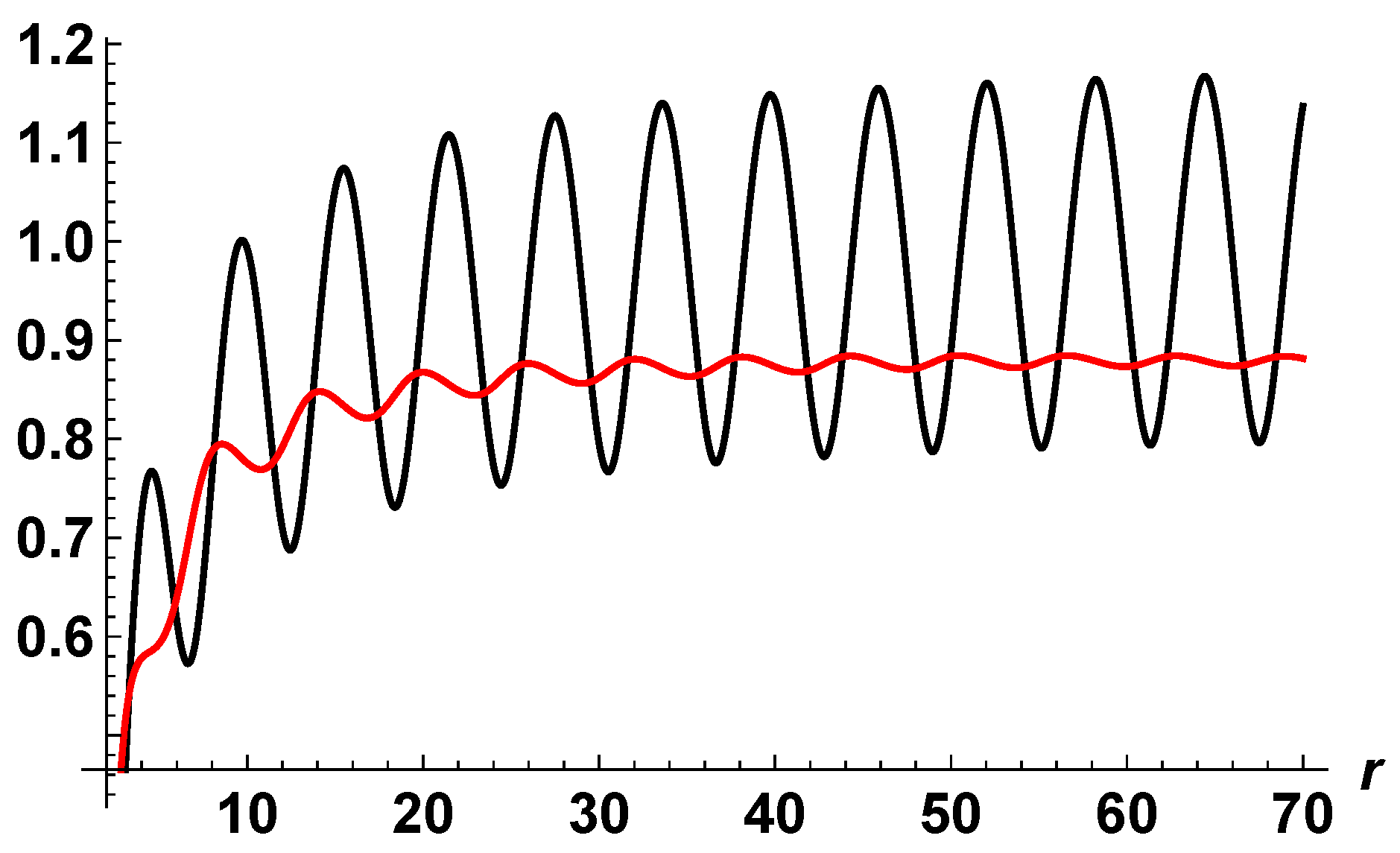
In particular, one is interested in inspecting all the local minima of the Euclidean action ${\mathcal{S}}_{\mathrm{E}}$ in the general class of all possible solutions of the field Equation (21). Although this is in general an enormous task, for our purpose, it is enough to show that typical Euclidean solutions of (21), like the ones displayed in Figure 1, have a stronger impact than the classical flat (perturbative vacuum) solution for which ${\mathcal{S}}_{\mathrm{E}}=0$ (note that there is no cosmological constant in this investigation). Indeed, extensive numerical investigation (obtained by changing various boundary conditions) shows that ${\mathcal{S}}_{\mathrm{E}}$ is in general negative and a lower bound is given by

$${\mathcal{S}}_{\mathrm{E}}\approx -4.07\pi \beta ,$$

(35)

with $\beta >0$. On the other hand, if $\beta <0$, ${\mathcal{S}}_{\mathrm{E}}=0$ always. A complete study of the phase diagram, including also the cosmological constant $\Lambda$, is beyond the purposes of this work.

5. Conclusions

One of the crucial issues that the Asymptotic Safety program has to face is to understand the physical structure of the ultraviolet theory emerging at the non-Gaussian fixed point. In the pure gravity case, there is a possible indication that the spectrum of the physical states is characterized by a linearised theory with a tachyon spin-2 field, instead of a ghost. The fate of this instability cannot be cured within the perturbation theory but most probably the ground state dynamically breaks both rotation and Lorentz invariance. This would clearly be a disaster from a phenomonological point of view unless typical oscillations periods and amplitudes are of the order of the Planck time and Planck length, as it seems to be the case near the NGFP. The relevant question is to understand the infrared behavior of these oscillation in order to make contact with laboratory and astronomical constraints. We hope to address this issue in a future work.

References

- Hornreich, R.M.; Luban, M.; Shtrikman, S. Critical Behavior at the Onset of k-Space Instability on the λ Line. Phys. Rev. Lett. 1975, 35, 1678–1681. [Google Scholar] [CrossRef]
- Bonanno, A.; Zappalà, D. Isotropic Lifshitz critical behavior from the functional renormalization group. Nucl. Phys. B 2015, 893, 501–511. [Google Scholar] [CrossRef] [Green Version]
- Savvidy, G.K. Infrared instability of the vacuum state of gauge theories and asymptotic freedom. Phys. Lett. B 1977, 71, 133–134. [Google Scholar] [CrossRef]
- Wetterich, C. Exact evolution equation for the effective potential. Phys. Lett. B 1993, 301, 90–94. [Google Scholar] [CrossRef] [Green Version]
- Reuter, M. Nonperturbative evolution equation for quantum gravity. Phys. Rev. D 1998, 57, 971–985. [Google Scholar] [CrossRef] [Green Version]
- Weinberg, S. Ultraviolet divergences in quantum theories of gravitation. In General Relativity: An Einstein Centenary Survey; Hawking, S.W., Israel, W., Eds.; Cambridge University Press: Cambridge, UK, 1979; pp. 790–831. [Google Scholar]
- Niedermaier, M.; Reuter, M. The Asymptotic Safety Scenario in Quantum Gravity. Living Rev. Relat. 2006, 9, 5. [Google Scholar] [CrossRef] [PubMed]
- Codello, A.; Percacci, R. Fixed Points of Higher-Derivative Gravity. Phys. Rev. Lett. 2006, 97, 221301. [Google Scholar] [CrossRef] [PubMed] [Green Version]
- Falls, K.; King, C.R.; Litim, D.F.; Nikolakopoulos, K.; Rahmede, C. Asymptotic safety of quantum gravity beyond Ricci scalars. Phys. Rev. D 2018, 97, 086006. [Google Scholar] [CrossRef] [Green Version]
- Benedetti, D.; Machado, P.F.; Saueressig, F. Asymptotic Safety in Higher-Derivative Gravity. Mod. Phys. Lett. A 2009, 24, 2233–2241. [Google Scholar] [CrossRef]
- Hamada, Y.; Yamada, M. Asymptotic safety of higher derivative quantum gravity non-minimally coupled with a matter system. J. High Energy Phys. 2017, 2017, 70. [Google Scholar] [CrossRef] [Green Version]
- Stelle, K.S. Renormalization of higher-derivative quantum gravity. Phys. Rev. D 1977, 16, 953–969. [Google Scholar] [CrossRef]
- Donoghue, J.F.; Menezes, G. Gauge assisted quadratic gravity: A framework for UV complete quantum gravity. Phys. Rev. D 2018, 97, 126005. [Google Scholar] [CrossRef] [Green Version]
- Falls, K.G.; Litim, D.F.; Schröder, J. Aspects of asymptotic safety for quantum gravity. arXiv 2018, arXiv:1810.08550. [Google Scholar] [CrossRef]
- Nitta, M.; Sasaki, S.; Yokokura, R. Spatially modulated vacua in a Lorentz-invariant scalar field theory. Eur. Phys. J. C 2018, 78, 754. [Google Scholar] [CrossRef]
- Bonanno, A.; Reuter, M. Modulated ground state of gravity theories with stabilized conformal factor. Phys. Rev. D 2013, 87, 084019. [Google Scholar] [CrossRef]
- Stelle, K.S. Classical gravity with higher derivatives. Gen. Relat. Gravit. 1978, 9, 353–371. [Google Scholar] [CrossRef]
- Bonanno, A.; Silveravalle, S. Characterizing black hole metrics in quadratic gravity. Phys. Rev. 2019, D99, 101501. [Google Scholar] [CrossRef]
Figure 1.
(black) and (red) obtained by solving the equations of motion of the quadratic theory as a function of the radial coordinate (in Planck units).
© 2019 by the author. Licensee MDPI, Basel, Switzerland. This article is an open access article distributed under the terms and conditions of the Creative Commons Attribution (CC BY) license (http://creativecommons.org/licenses/by/4.0/).
Share and Cite
MDPI and ACS Style
Bonanno, A. On the Structure of the Vacuum in Quantum Gravity: A View from the Asymptotic Safety Scenario. Universe 2019, 5, 182. https://doi.org/10.3390/universe5080182
AMA Style
Bonanno A. On the Structure of the Vacuum in Quantum Gravity: A View from the Asymptotic Safety Scenario. Universe. 2019; 5(8):182. https://doi.org/10.3390/universe5080182
Chicago/Turabian StyleBonanno, Alfio. 2019. "On the Structure of the Vacuum in Quantum Gravity: A View from the Asymptotic Safety Scenario" Universe 5, no. 8: 182. https://doi.org/10.3390/universe5080182
Note that from the first issue of 2016, this journal uses article numbers instead of page numbers. See further details here.