Inhomogeneous Jets from Neutron Star Mergers: One Jet to Rule Them All

Abstract

Using the resultant profiles from 3D hydrodynamic simulations of relativistic jets interacting with neutron star merger wind ejecta, we show how the inhomogeneity of energy and velocity across the jet surface profile can alter the observed afterglow lightcurve. We find that the peak afterglow flux depends sensitively on the observer’s line-of-sight, not only via the jet inclination but also through the jet rotation: for an observer viewing the afterglow within the GRB-bright jet core, we find a peak flux variability on the order <$0.5$ dex through rotational orientation and <$1.3$ dex for the polar inclination. An observed afterglow’s peak flux can be used to infer the jet kinetic energy, and where a top-hat jet is assumed, we find the range of inferred jet kinetic energies for our various model afterglow lightcurves (with fixed model parameters), covers ∼1/3 of the observed short GRB population. Additionally, we present an analytic jet structure function that includes physically motivated parameter uncertainties due to variability through the rotation of the source. An approximation for the change in collimation due to the merger ejecta mass is included and we show that by considering the observed range of merger ejecta masses from short GRB kilonova candidates, a population of merger jets with a fixed intrinsic jet energy is capable of explaining the observed broad diversity seen in short GRB afterglows.

1. Introduction

The afterglows that follow short-duration Gamma-Ray Bursts (GRBs) are powered by decelerating, relativistic jets. The likely progenitor system for short GRBs is the merger of binary neutron stars or neutron star–black hole binaries (see [1,2,3] for a review of short GRBs); for such a compact binary merger origin, the power available for the jets is expected to be on the order of ${10}^{51}$ erg s⁻¹, with quite a narrow distribution [4,5]1. However, the jet parameters inferred via afterglow studies reveal a diverse population in terms of energy, as well as environment and microphysics, such as the fraction of energy that contributes to the magnetic field or particle acceleration [6,7], and this broad distribution in inferred kinetic energy can be difficult to reconcile with the narrow, theoretically expected range.

A jet launched following a compact stellar merger will propagate through the merger ejecta and winds (e.g., [8,9,10,11,12,13,14,15,16,17,18]), this results in the collimation of the jet before breakout [19,20,21,22]. As a consequence of the turbulent motions arising during the hydrodynamic interaction between the jet and the surrounding ejecta, the resultant jet will have an angular shape that is independent of the injected jet structure [16], unless the ejecta density is very low or the jet power very high [18]. The different initial conditions between these two studies make a direct comparison non-trivial; whereas Nativi et al. [16] use initially “warm” jets, Urrutia et al. [18] have initially “cold” jets and include a broader jet luminosity distribution. Additionally, we note that the turbulent effects seen in 3D simulations are significantly reduced in 2D (see [23]); thus the turbulent destruction of the initial jet structure seen in the 3D hydrodynamic simulations by Nativi et al. [16] is not as pronounced in the 2D hydrodynamics used by Urrutia et al. [18]. However, unlike the functional form of the resultant jet structure profile due to this turbulence, the characteristic opening angle of the emergent jet can retain information about the injected jet’s angular width (e.g., [9]).

A universal, or quasi-universal, jet structure profile for GRB jets with a standard energy reservoir was first proposed by Lipunov et al. [24] and expanded upon by Rossi et al. [25], Zhang and Mészáros [26]. For such universal structured jet models, the broad range in observed GRB energies is a result of the arbitrary viewing angle. Analysis of the spectral peak energy to isotropic energy correlations for a population of such universal GRBs can be used to constrain the viable jet structure profile (e.g., [27,28,29]). For long GRBs, classically associated with a collapsar origin, the luminosity function can be used to exclude some shallower jet structure profiles [30], however, empirical correlations may well be a result of an apparent jet structure [31], and consistent with the resultant structure profiles from simulations of jets in massive stars (e.g., [32]). Additionally, observational signatures for the presence of jet structure within GRB-producing jets are contained within the various afterglow lightcurve decline rates and breaks [33,34,35,36].

As GRBs are highly beamed, their afterglows are preferentially selected to be at small inclination angles to the line-of-sight, $\iota$, where the emission is brightest [37]. For such GRBs, the afterglow lightcurve can be modelled using a simple top-hat jet structure, where any angular dependence of the energy or velocity is ignored, resulting in a uniform jet within a cone defined by the jet’s opening angle, ${\theta }_c$ (see discussion in [38]). However, where a top-hat jet structure model is assumed, the inferred energy from lightcurve fits will return kinetic energy values equal to the average energy of the intrinsic jet structure profile within the $1/\Gamma$ beaming cone and likely not the true or maximum energy of the jet. Typically, $1/\Gamma <{\theta }_c$ at peak flux time where the observer’s line-of-sight is $\iota \lesssim {\theta }_c$—where $\Gamma$ is the bulk Lorentz factor of the emitting region at the observation time. This should not be confused with higher inclination cases, where the GRB is either absent or at a much lower luminosity, e.g., the expected afterglow counterparts to gravitational wave detected mergers (see [39,40] for details of such “off-axis” observed afterglows). Here we use the results of 3D hydrodynamic simulations of jets propagating through the merger ejecta and neutrino-driven winds of a neutron star merger (see, [15,16,41]) to investigate the effects of inhomogeneity within the jet’s energy and velocity profile on the afterglows of short GRBs.

In Section 2 we describe our method for modelling the resultant jet profiles from the simulations relevant to the bright GRB emitting population of short bursts. In Section 3, we show the diversity of afterglow lightcurves from a single jet simulation as a function of observer line-of-sight relative to both inclination and rotation. Additionally, we use the simulation jet structure results to generate a general, analytic function for the typical structure of a short GRB jet and compare the flux density for the afterglow from this model to the short GRB afterglow population. These results are discussed in Section 4, where we approximate how the ejecta mass responsible for a thermal kilonova (e.g., [42,43]) can alter the effective core-size of the jet and show how this compares to a selection of typical afterglow lightcurves for short GRBs with candidate kilonovae. Our conclusions are listed in Section 5.

2. Method

The energy per steradian and Lorentz factor at each point of a surface that describes the afterglow-producing jet can be extracted from simulations. We use two ultra-relativistic jet simulations from [16], and determine the typical Lorentz factor for each surface element from the mass-averaged radial profile for $h\Gamma >2$ at a given polar angle, $\theta$, and rotational angle, $\varphi$—where h is the specific enthalpy which gives a measure of the sum of the system’s internal energy and the product of pressure and volume, and $\Gamma$ the Lorentz factor. The two simulations we utilise are identical but for the structure of the injected jet in each case; the first uses a ‘top-hat’ structured jet with a uniform energy and enthalpy until a sharply cut-off edge, and the second uses a profile described by a Gaussian function. Both jets have a power, $L_{\mathrm{j}}\sim {10}^{50}$ erg s⁻¹, and are labelled th50 and gs50, respectively.

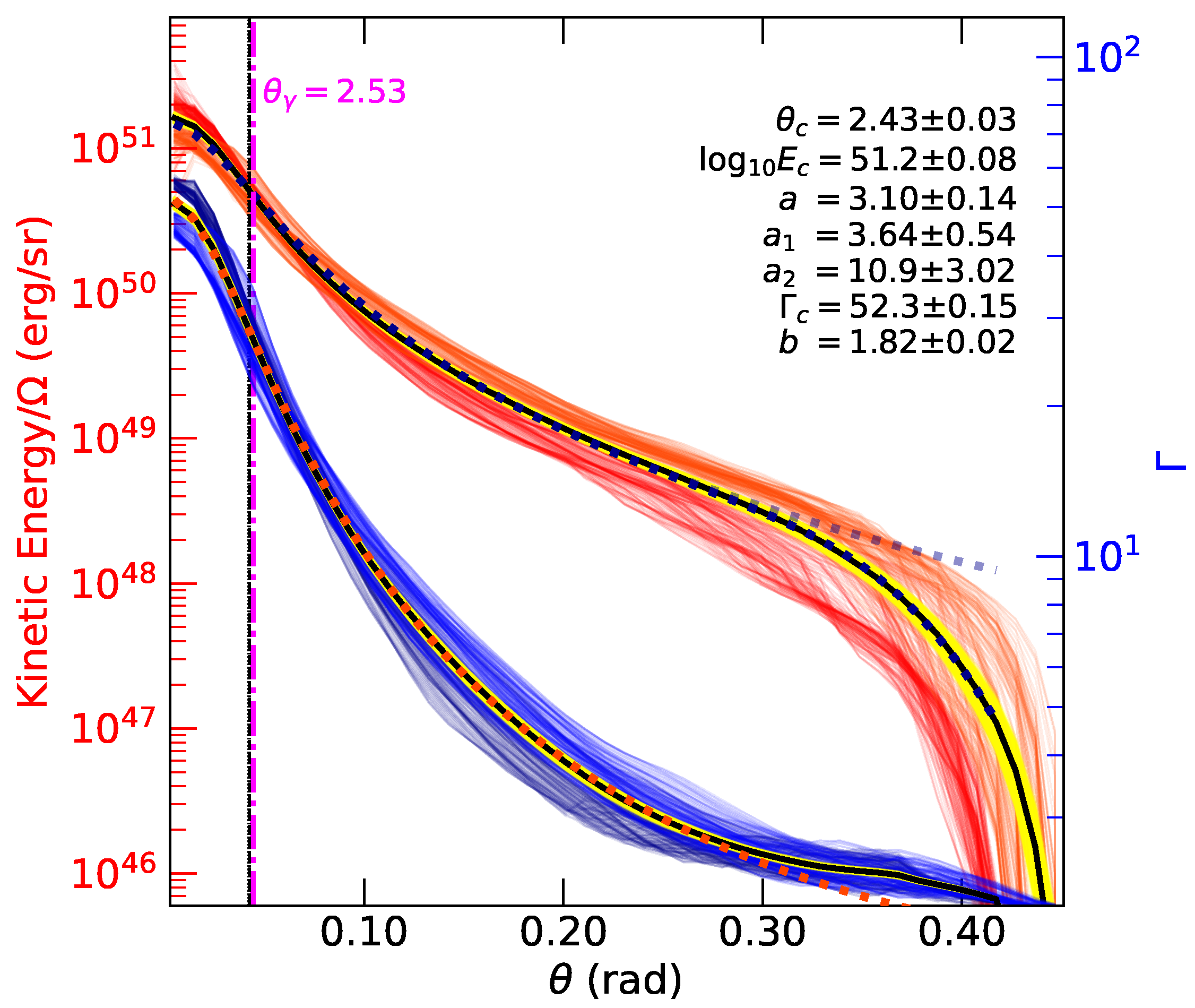
The two left panels in Figure 1 show the face-on distribution of energy and Lorentz factor for each simulation output once ballistic expansion is achieved, i.e., the system has stopped acceleration and is cold with $(h-1)<1$ everywhere on the grid. The right panels show energy (red) and Lorentz factor (blue) with polar angle where the shaded regions indicate the maximum to minimum range for each parameter with rotation through $\varphi$ on the jet surface at the given angle $\theta$. We can approximate the mean of these profiles analytically using (e.g., [44]):

$$\begin{array}{ccc}\hfill \Theta & =& {\left[1+{\left(\frac{\theta }{{\theta }_c}\right)}^2\right]}^{1/2},\hfill \end{array}$$

(1)

$$\begin{array}{ccc}\hfill E\left(\theta \right)& =& E(\theta =0){\Theta }^{-a},\hfill \end{array}$$

(2)

$$\begin{array}{ccc}\hfill \Gamma \left(\theta \right)& =& 1+\left[\Gamma (\theta =0)-1\right]{\Theta }^{-b}.\hfill \end{array}$$

(3)

We use a linear regression fit to the mean for both the energy and Lorentz factor profiles within an angle ${\theta }_j=0.42$ rad, or ∼${24}^{\circ }$. The energy profile is cut-off2 using the functional form ${(1+{(\theta /{\theta }_j)}^{a_2})}^{-a_1}$. The model jet structure (Equations (1)–(3)) fit parameters to the mean through rotation for the simulation profiles are shown in

Table 1. Analytic jet structure profile parameters, see Equations (1)–(3) plus text, from fits to the mean energy and Lorentz factor with polar angle for each simulation and the averaged profile, see Section 3.

Model	${\mathit{\theta }}_{\mathit{c}}$ (rad)	$log\left({\mathit{E}}_{\mathit{c}}\right)$ (log erg sr−1)	${\mathit{\Gamma }}_{\mathit{c}}$	a	${\mathit{a}}_1$	${\mathit{a}}_2$	b
th50	$0.0428\pm 0.0007$	$51.27\pm 0.11$	$58.0\pm 0.2$	$3.50\pm 0.20$	$7.89\pm 0.94$	$14.79\pm 3.14$	$1.98\pm 0.03$
gs50	$0.0415\pm 0.0004$	$51.10\pm 0.06$	$45.6\pm 0.1$	$2.82\pm 0.10$	$3.96\pm 0.45$	$12.48\pm 2.59$	$1.62\pm 0.01$
Averaged	$0.0424\pm 0.0005$	$51.18\pm 0.08$	$52.3\pm 0.2$	$3.10\pm 0.14$	$3.64\pm 0.54$	$10.90\pm 3.02$	$1.82\pm 0.02$

.

To test how the inhomogeneity of the jet surface affects the observed afterglow lightcurves for various lines of sight, we generate afterglows at a fixed emission frequency for observers at different combinations of polar and rotational angles. The afterglows are calculated using the method described in [36,39,45]. We use the energy and Lorentz factor for each surface element from the simulation output and calculate the afterglow contribution from each, as seen by an observer at a given inclination, $\iota$, and observer time, $t_{\mathrm{obs}}$, and sum the equal time contributions to give the total observed flux with observer time, i.e., we integrate over the equal arrival time surface. This is the current standard for structured jet afterglow models (e.g., [45,46]), however, we note that this assumes the jet surface profile is frozen until lateral expansion begins. As the outflow has a very low enthalpy, i.e., $(h-1)<1$, at the time we sample the jet profile, the frozen-in assumption is a reasonable approximation until the outflow begins deceleration (see also [47]). Hydrodynamic simulations of relativistic jets show that lateral spreading only becomes significant at late times during the afterglow emission phase, (e.g., [48]), thus we expect no significant changes to the jet surface profile until very late times.

The lightcurves for each $\varphi$ element at a discrete polar angle in the range $(0.0\le \theta \le 6.0)\times {\theta }_c$ for the two simulation models are shown in Figure 2. The lightcurves are calculated at an observed frequency, $\nu =3.8\times {10}^{14}$ Hz, where for simplicity we assume redshift, $z=0$, and a luminosity distance, $D_L=100$ Mpc. The afterglow model microphysical parameters are fixed at ${\epsilon }_e=\sqrt{{\epsilon }_B}=0.1$, an electron distribution index, $p=2.15$, an ambient medium particle number density, $n=1$ cm⁻³, and a $\gamma$-ray efficiency of $\eta =0.15$, where we assume a fixed efficiency throughout the jet.

The emission of $\gamma$-rays from a jet requires the source to be optically thin which places physical constraints on the angular profile from which a GRB can be emitted/observed (e.g., [39]). Viable locations for $\gamma$-ray emission can be determined using a relation between energy and Lorentz factor that considers the opacity of the medium to gamma-rays. The minimum Lorentz factor for an optically thin medium considering only the scattering by electrons that accompany baryons in the jet is (e.g., [49,50]):

$${\Gamma }_{\min }={\left(\frac{{\sigma }_{\mathrm{T}}}{32m_{\mathrm{p}}\pi c^4}\frac{L_{\gamma ,\mathrm{iso}}(1+z)}{\delta t}\right)}^{1/6},$$

(4)

which is consistent with ${\Gamma }_{\min }\propto {E_{\gamma ,\mathrm{iso}}}^{0.17}$ found in [51]. Here, ${\sigma }_{\mathrm{T}}$ is the Thompson cross-section, $m_{\mathrm{p}}$ is the proton mass, c is the speed of light, and the variables: $L_{\gamma ,\mathrm{iso}}$ is the isotropic equivalent $\gamma$-ray luminosity, z is the source redshift, and $\delta t$ is the minimum variability timescale. The observed isotropic equivalent $\gamma$-ray energy can be approximated from the luminosity as, $E_{\gamma ,\mathrm{iso}}=L_{\gamma ,\mathrm{iso}}{T}_{\mathrm{dur}}$, where $T_{\mathrm{dur}}$ is the burst duration3. The total energy is then $E=E_{\gamma ,\mathrm{iso}}/\eta$, where $\eta$ is the efficiency of the $\gamma$-ray emission. A basic approximation of the energy per steradian for the outflow with a given $\Gamma$ to be $\gamma$-ray bright is then

$$\frac{E}{\Omega }\lesssim {\left(\frac{\Gamma }{10}\right)}^6\left(\frac{\delta t}{0.1\mathrm{s}}\right)\left(\frac{T_{\mathrm{dur}}}{0.1\mathrm{s}}\right){\left(\frac{\eta }{0.15}\right)}^{-1}\times {10}^{48}\mathrm{erg}/\mathrm{sr},$$

(5)

where all timescales are measured in the lab frame. Equation (5) provides a conservative estimate for the jet regions that can emit GRBs and the dependence on the burst duration, e.g., engine timescale, minimum variability timescale, and $\gamma$-ray efficiency.

3. Results

We have generated afterglow lightcurves from the resultant energy and Lorentz factor surface profiles for two 3D hydrodynamic simulations of jets propagating through neutron star merger winds for observers at various $\theta$ and $\varphi$ relative to the jet central axis (see [15,16] for simulation details). The effects of the jet orientation to the line-of-sight on the peak afterglow flux, for emission in the regime ${\nu }_m<\nu <{\nu }_c$, where ${\nu }_m$ is the characteristic synchrotron peak frequency and ${\nu }_c$ is the cooling frequency, is shown in Figure 3 for observers within the $\gamma$-ray emitting region of the jet (as defined by Equation (5)). The maximum variation in the peak flux at a fixed inclination but through a $2\pi$ rotation in $\varphi$ is ∼$0.5$ dex seen for the gs50 model. The th50 model has less overall variation, with ∼$0.2$ dex in peak afterglow flux, where dex is the decimal exponent. The most significant change in peak flux is seen with inclination from the jet central axis, where for both th50 and gs50 the peak flux varies by ∼$1.3$ dex within the approximate $\gamma$-ray emitting region.

For GRB afterglows, the kinetic energy of the jet is found via afterglow modelling which typically assumes an outflow with a uniform, or top-hat, energy distribution (e.g., [6]). The results of our simulations show that the jets that produce GRB afterglows do not have a uniform energy profile, and that orientation through both $\theta$ and $\varphi$ can change the kinetic energy inferred from simple afterglow models. For GRB afterglows with ${\nu }_m<\nu <{\nu }_c$ the peak flux is $F_p\propto {E_{\mathrm{k}}}^{(3+p)/4}$, where $F_p$ is the afterglow peak flux, $E_{\mathrm{k}}$ is the kinetic energy, and p is the power-law distribution index for accelerated electrons [52]—note that we ignore the dependence on the ambient medium density, n, and the microphysical parameters, ${\epsilon }_B$ and ${\epsilon }_e$ as these quantities are fixed for our sample. Figure 4 shows the kinetic energy distribution, as inferred by a distant observer and weighted for a randomly oriented source with inclination $\iota \le {\theta }_{\gamma }$, for each of our jet simulations in comparison to the observed kinetic energy distribution for the population of short GRBs as listed in [6]. The afterglow lightcurves were calculated assuming a fiducial efficiency for $\gamma$-rays of $\eta =0.15$, where the energy in the jet is $E=E_{\gamma }+E_{\mathrm{k}}$, with $E_{\gamma }$ being the energy radiated in $\gamma$-rays. The dashed histogram shows the distribution assuming an efficiency, $\eta =0.85$, resulting in a lower typical energy distribution as more energy is lost via the GRB. The dash-dotted lines show the isotropic equivalent kinetic energy for each of our jets, calculated assuming the core angle listed in Table 1 contains all of the initial jet energy. The logarithmic kinetic energy distribution inferred from a single jet model covers ∼third of the observed short GRB population. As we have artificially fixed the $\gamma$-ray efficiency for the entire emitting region, our distribution is likely significantly narrower than one with a more realistically determined efficiency, e.g., $\eta (\theta ,\varphi )$, that varies according to local conditions across the jet’s surface.

The two 3D simulations highlight that the form of the resultant jet profiles are largely a result of fluid instabilities in the jet-wind interaction regions [16], however, for lower density winds4, or much more powerful jets, the injected jet structure can be partially preserved [18]. By using the rotation in $\varphi$ for each surface to produce an energy and Lorentz factor profile in $\theta$ we can find an average jet structure profile from our simulations that includes the rotational variation seen here. We use a bootstrapping technique, re-sampling these unique jet profiles, to produce a sample of mean profiles and then find the mean of this new sample. Equations (1)–(3) are fit to this mean profile, including the energy cut-off described in Section 2, via linear regression to find the best-fit parameters. These are listed in Table 1 as ‘Averaged’ and shown in Figure 5 along with the initial profiles.

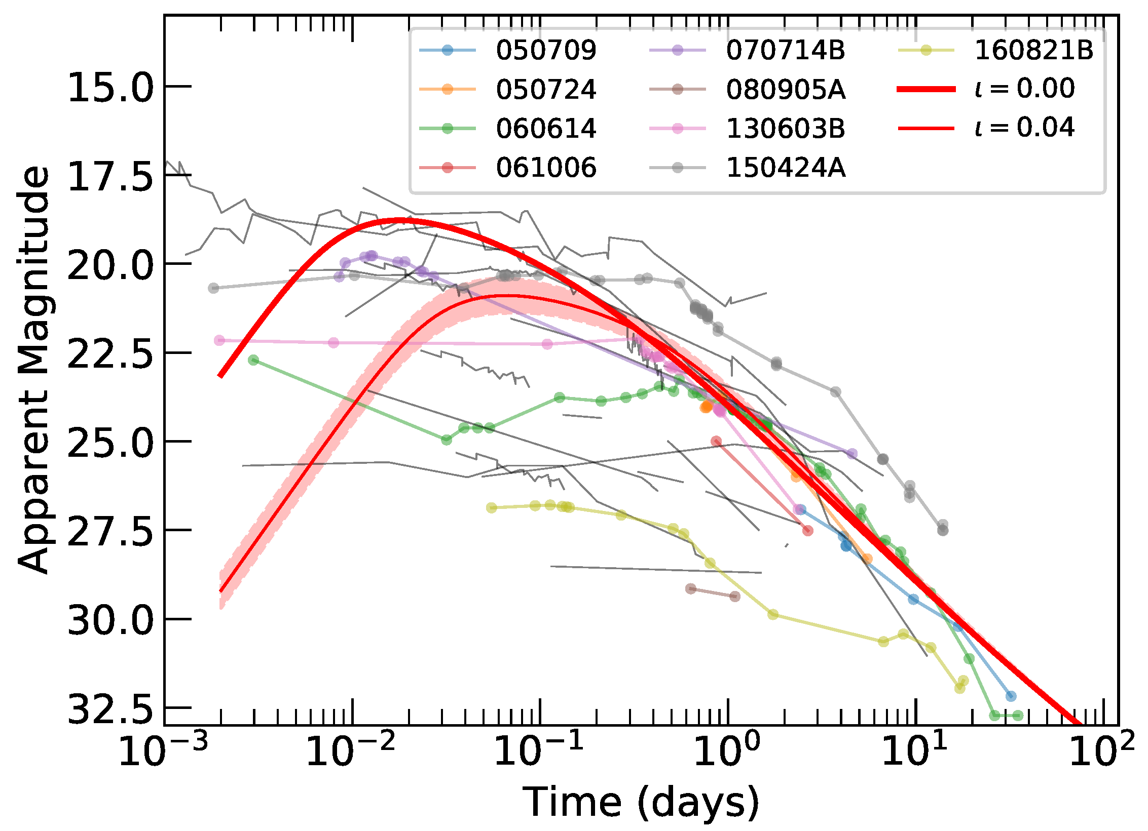
The afterglows from our averaged jet structure profile are compared to the observed short GRB population in Figure 6. Here we show, in red, the model $R_C$-band afterglow for a source at $z=1$ using the same fiducial parameters as the earlier models. Individual lightcurves are shown for an observer that is either aligned with the jet central axis, or at $\iota ={\theta }_{\gamma }$, the maximum angle at which $\gamma$-rays are emitted for our model; these cover the range of expected GRB afterglows from a jet with our structure and fixed parameters. The sample of 30 individual short GRBs (grey and coloured lines) are optical afterglows for bursts with a measured redshift; each afterglow is a composite of various filters that have been shifted using the spectral energy distribution for each burst and corrected for Galactic foreground extinction and host contribution (if necessary and possible) to produce an observed $R_C$-band lightcurve for a source at redshift $z=1$ (see [53,54] and references therein).

The post-jet-break decline for our model lightcurves is consistent with the tail of the short GRB population, and the peak of the model afterglows agrees nicely with the brightest in this distribution—we note that short GRB afterglows shown here may include contributions from extended prompt emission, the reverse shock, energy injection, and kilonova. Our afterglow models have a fixed ambient density, $n=1$ cm⁻³, and microphysical parameters, ${\epsilon }_e=\sqrt{{\epsilon }_B}=0.1$ and $p=2.15$; allowing these to vary would change both the timescale and the peak flux of the afterglow, with the deceleration (or peak) time, $t_d\propto {E_{\mathrm{k}}}^{1/3}{n}^{-1/3}{\Gamma }^{-8/3}$, and $F_p\propto E_{\mathrm{k}}{\Gamma }^{2(p-1)}{{\epsilon }_B}^{(1+p)/4}{{\epsilon }_e}^{p-1}{n}^{(1+p)/4}$, where $\Gamma$ is the bulk Lorentz factor at the deceleration radius and the emitting frequency is in the regime, ${\nu }_m<\nu <{\nu }_c$.

4. Discussion

We have used the results from 3D hydrodynamic simulations of relativistic jets interacting with neutron star merger winds to show the effect on the observed afterglow, in terms of the peak flux, from the inhomogeneity of the resultant jet structure in both polar, $\theta$, and rotational, $\varphi$, orientations. We have shown that for an observer viewing the jet at $\iota \le {\theta }_{\gamma }$, the rotational orientation of the jet surface, $0\le \varphi \le 2\pi$ results in an afterglow peak flux with a scatter of $\Delta \lesssim 0.5$ dex. The structure through the polar-angle, $0\le \iota \le {\theta }_{\gamma }$, results in a larger scatter for the peak afterglow flux of $\lesssim 1.3$ dex, as expected from previous studies of jet structure on the afterglows to merger jets which only considered the polar variation in jet properties [39,40]. For the scatter in flux density due to the rotational orientation, the deviation from the mean gradually reduces with time and follows the expected change in beaming angle; the flux changes by a factor $\lesssim 1+(\Delta /2-1)\times min{\left[1,(t_d/t)\right]}^{3/8}$, where $t_d$ is the deceleration time, and t is the observer time since burst.

The jet’s kinetic energy, as inferred via afterglow modelling, will be broader than that assumed from a simple uniform jet model. For our two fiducial models, we find the inferred kinetic energy distribution covers $\gtrsim 1$ dex in energy for a fixed $\gamma$-ray efficiency, $\eta$. More realistically, $\eta$ would vary as a function of both the energy and Lorentz factor with $\theta$ and $\varphi$, where at lower Lorentz factors some fraction of the energy dissipated within the jet will be reabsorbed (see, [55,56]) and the effective $\eta$ would be smaller. Higher energy regions may result in more efficient shocks (e.g., [55]) and the $\eta$ could be larger—similarly, for photospheric emission during the prompt emission of GRBs, Gottlieb et al. [57] find a higher efficiency in more energetic regions. Such properties would further broaden the inferred kinetic energy distribution from a jet with fixed energy and we encourage further investigations into a physically motivated expression for $\eta (E,\Gamma )$ in GRB outflows.

The core angle, ${\theta }_c$, from the fits to the mean energy and Lorentz factor profiles for Equations (1)–(3), see Table 1, returns a remarkably similar value to that inferred via modelling the afterglow jet-break time in [16] using the same simulation data but a rotationally averaged jet profile. For jet simulations such as these, the core or jet opening angle is often presented as the average angle within which material has $h\Gamma >10$ (e.g., [9]). Using this method with our 3D simulations, we find a ${\theta }_{\mathrm{average}}=0.1058$ and $0.1278$ rad for the th50 and gs50 models, respectively. These are both larger than the values found via profile fitting or the jet-break time by a factor $\sim 2.5$–3. This suggests that the apparently narrower jets from our simulations are merely a result of the way ${\theta }_c$ is estimated. Such narrow jets are well within the observed range for opening angles5 inferred from the short GRB population (e.g., [59,60]).

The degree of the jet collimation for a GRB producing jet, and the resultant jet opening angle is a complicated function of the jet’s power, the density of the medium through which the jet is propagating, and the jet’s initial opening angle [19]. The details of how to estimate the final jet opening angle from a set of initial conditions and for an expanding medium are described by [22], (see also [11,21] etc.). The degree of collimation is shown to be dominantly proportional to the ratio of jet power and ambient medium mass, $\theta /{\theta }_0\propto {(L_j/M_{\mathrm{a}})}^{1/4}$, where $\theta$ is the resultant opening angle, ${\theta }_0$ is the injected jet’s opening angle, $L_j$ is the jet power, and $M_{\mathrm{a}}\equiv M_{\mathrm{ej}}$ is the mass of the ambient medium/winds through which the jet is propagating and equivalent to the ejecta mass for a neutron star merger. The exact relation depends on how the medium is expanding, the ratio of the energy density for the jet to ejecta, and weakly on the timescale. Additionally, particle effects such as neutron conversion-diffusion may contribute to the resultant jet structure [61].

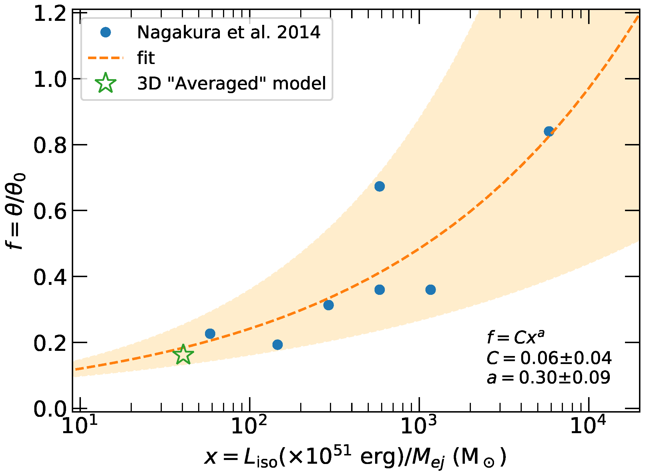
The afterglows to short GRBs indicate that they are accompanied by a broad diversity of kilonovae (e.g., [62,63]). Model fits to GRB afterglows with kilonova candidates suggest that the population ejecta mass distribution has a scatter of $\Delta log{M}_{\mathrm{ej}}\lesssim 1$, a broad uncertainty on the ejecta velocity, $v_{\mathrm{ej}}\le 0.3$c, and a several orders of magnitude range for the Lanthanide fraction [64]. Theoretical studies of kilonova models show an equally diverse range of possible parameters (e.g., [65]). The mass and velocity of the ejecta, and the power and initial opening angle of the jet have an influence on the resulting jet opening angle—to approximate these factors, we take the results of 2D hydrodynamic simulations for a variety of initial jet and ejecta compositions from [9] and fit a power-law function, $\theta /{\theta }_0\propto {(L_j/M_{\mathrm{ej}})}^a$, to determine the index a for the scaling. The results are shown in Figure 7, where we have used the isotropic equivalent luminosity for the initial jet. The opening angle, as inferred from jet profile fitting, for our averaged jet structure model is shown as a star. The fit index $a=0.30\pm 0.09$ is within error of the theoretically expected, $a=0.25$, where we ignore the timescale and ejecta expansion dependence [66].

Using the fit for the scaling relation ${\theta }_c/{\theta }_0\propto {(L_j/M_{\mathrm{ej}})}^a$ shown in Figure 7, the core angle for a structured jet with our ‘Averaged’ jet profile, as a function of the jet energy and/or the ejecta mass, is

$$\frac{{\theta }_c}{{\theta }_0}=0.1696{\left[\frac{E_j/1.7\times {10}^{49}\mathrm{erg}}{M_{\mathrm{ej}}/0.072M_{\odot }}\right]}^{0.3}\mathrm{rad},$$

(6)

where $E_j$ is the equivalent energy for the jets calculated assuming the isotropic equivalent core energy at $\theta =0$ and a top-hat jet with an opening angle ${\theta }_j\equiv {\theta }_c$, e.g., $E_j=E_{\mathrm{iso}}(\theta =0){\theta }_c^2/2$, thus ensuring that the jet core energy is uniform between cases, $M_{\mathrm{ej}}$ is the mass of the ejecta/wind, and ${\theta }_0$ the initial (injected) jet’s half opening angle (in our simulations ${\theta }_0=0.25$ rad).

Comparison to Sources with Kilonova Candidates

Figure 6 shows our sample of 30 composite short GRB afterglows normalised to $z=1$ [53,54]. The GRBs with kilonova candidates within this sample have coloured lines, points marking the data, and a corresponding legend identifier. These kilonova candidate GRBs are additionally listed in

Table 2. Short GRBs with kilonova candidates. Estimated ejecta masses are from the respective reference column—where more than one mass is listed, the values are in the reference order; the bold value is that used to determine the jet collimation for the models shown in Figure 8. GRBs 150101B and 200522A, below the line, are not included in our optical lightcurve sample. The 4th and 5th columns show the value of index p used for the model afterglow lightcurves, and the relevant reference. The last three columns show the opening angle, the isotropic equivalent kinetic energy, inferred from the jet structure in each case, and the ambient particle density used for the lightcurves in Figure 8. The ejecta mass ($M_{\mathrm{ej}}$) is in units M_⊙, core angle (${\theta }_c$) is in radians, kinetic energy ($E_{\mathrm{k}}$) is in erg, and the ambient density (n) in cm⁻³.

GRB	${\mathit{M}}_{\mathbf{ej}}$	Ref.	p	Ref.	${\mathit{\theta }}_{\mathit{c}}$	${\mathit{E}}_{\mathbf{k}}$$\times {10}^{52}$	$log\mathit{n}$
050709	0.05	[64,67]	2.31	[6]	0.047	1.29	−3.00
050724	0.001	[68]	2.29	[6]	0.160	0.11	−1.00
060614	0.077, 0.1	[64,67]	2.40	[69]	0.042	1.69	−3.30
061006	0.01	[68]	2.39	[6]	0.078	0.48	−2.30
070714B	0.01	[68]	2.30	[6]	0.078	0.48	−0.30
080905A *	0.007	[64]	2.06	[6]	0.043	0.16	−2.15
130603B	0.03, 0.01–0.1, 0.075	[64,67,70]	2.70	[6]	0.056	0.94	−1.00
150424A	0.1	[64]	2.30	[64]	0.040	1.86	−1.40
160821B *	0.01, 0.17, <0.006	[60,64,71]	2.30	[60]	0.038	0.20	−2.00
150101B	>0.02, >0.1, 0.037	[64,72,73]	–	–	–	–	–
200522A	0.1	[74]	–	–	–	–	–

* indicates a GRB where we reduced our jet model energy by a factor 10.

, with the literature values for merger ejecta masses inferred from model fits/estimates to observations by the listed reference.

Figure 8 shows the 9 kilonova candidate GRB afterglows in our sample. For each GRB we use the ejecta mass value listed in bold from Table 2 to estimate a new jet core size using Equation (6). As we keep the jet core energy constant, changing the model core size will result in a different isotropic equivalent kinetic energy for the jet structure model profile. The new isotropic equivalent kinetic energy, for the $\theta =0$ point, is found assuming the core energy in the jet from our ‘Averaged’ model is conserved, so $E_{K,\mathrm{iso}}(\theta =0)=(1-\eta )1.9\times {10}^{52}(1.79\times {10}^{-3}/{\theta }_c^2)$, where $\eta$ is the efficiency of the $\gamma$-ray emission, and ${\theta }_c$ is the new core angle. These new values for ${\theta }_c$ and central isotropic equivalent energy are then used to substitute the values in our ‘Averaged’ jet structure profile shown in Figure 5.

In Figure 8, model lightcurves shown with a red line have fixed microphysical parameters, ${\sqrt{\epsilon }}_B={\epsilon }_e=0.1$, and where the model lightcurve is shown with a green line, we change to ${\epsilon }_B=0.1$ to give better agreement with the data. For each lightcurve we use values for the index p from the literature, as listed in Table 2. For each GRB afterglow we vary the value of the ambient density to find an approximate alignment between our fiducial model and the afterglow data6. For GRBs 080905A, and 160821B, we could not find a satisfactory alignment using our total jet energy and varying only the ambient density. However, as described in [60], GRB 160821B requires an initially low-power jet that is refreshed at later times7. The equivalent energy of the initial jet in GRB 160821B is ∼0.1 that of our fiducial jet, however, the energy injection at ≳1 days for GRB 160821B results in a total energy that is consistent with the energy of our single episode jet model (see [60] for details). We apply this same reduction in initial jet energy to GRB 080905A to achieve a better alignment with the observed flux density. Our model lightcurves do not include the refreshed shock contribution, however, for GRB 160821B this is equivalent to the late time ‘excess’ seen in the data. No data, other than the non-constraining upper-limits, at ≳10 days is available for GRBs 080905A to test the refreshed shock scenario.

The model afterglows in Figure 8 also show the maximum variability due to the rotational orientation of the jet with respect to the observer, as shown in Figure 3—note that this uncertainty in peak flux does not affect the on-axis case. The angle ${\theta }_{\gamma }$ provides an indication of the highest angle from which an observable GRB is likely to be emitted, however, this is not a hard limit and where beaming effects, the distance to the source, and secondary $\gamma$-ray emitting components are considered, e.g., shock breakout of the cocoon, then the inclination at which an observer could detect the GRB is higher for nearby sources.

The lightcurves for GRBs 050724, 060614 and 150424A stand out in our sample as having a late break to the steep decline phase when compared with our fiducial models, and the green lightcurves shown in Figure 8 have used ${\epsilon }_B=0.1$ to give better agreement with the data—additionally noting that the choice of initial jet energy in our simulation was arbitrary8. The opening angle for these jet models relies on the ejecta mass estimates, and for GRB 050724, the value of $0.001$ M_⊙ is the smallest in our sample and may well be underestimated. GRB 060614 is technically a long-duration GRB, with a prompt burst episode lasting ∼100s, however, the absence of an accompanying bright supernova combined with it exhibiting an initial spike of gamma-rays with a duration of only a few seconds has led to speculation that it could have been produced by a compact binary merger [53,75,76,77]. The differences in these GRBs (noting that GRB 150424A which has a large uncertainty on the source redshift, e.g., [78]) may indicate that these bursts have a different progenitor to typical short GRBs, i.e., they may be the result of a neutron star-black hole merger as opposed to a binary neutron star merger (e.g., [79]), where the potential energy budget for the jet is marginally higher (e.g., [4]) or the ejecta mass is lower, especially in the polar regions, resulting in a potentially wider emergent jet structure.

The compact stellar merger origin for short GRBs has a limited energy budget for the jets, typically of the order ∼${10}^{51}$ erg for neutron star mergers [5]. Yet the observed distribution for the energy in the short GRB population spans $\sim 4$ orders of magnitude, see Figure 4 and [6]. Here we have shown that inhomogeneity in the energy and velocity distribution across an emergent jet’s surface due to turbulent processes via jet-ejecta mixing can account for a significant fraction of the observed spread in inferred kinetic energies. By taking into account the range of ejecta masses from the candidate kilonova population, the effective opening angle (the jet core angle in our notation) for a GRB jet with a fixed, or limited, energy budget can be determined. When combined with the expected variation in the ambient density between sources we can explain much of the variety in afterglow flux and timescales for the small sample of GRBs with kilonova candidates.

Figure 2, where $\iota \sim 4-5{\theta }_c$, and fits for the rotationally averaged simulation jet structure profiles in [16] show that such a functional jet structure is additionally consistent with the afterglow of GW170817/GRB 170817A—we do not repeat that analysis here. For the afterglow to GRB 170817A, multiple jet structure profiles have shown viable fits to the data, including more exotic structures than the core-dominated profiles presented here (e.g., [80]), as well as the refreshed shock/energy injection scenario [81]. Several authors have shown how the jet structure profiles used to explain the lightcurve of the afterglow of GRB 170817A resemble the cosmological population of short GRB afterglows when viewed at a very small inclination (e.g., [82,83,84,85]), thus renewing the case for a universal jet structure profile for merger jets (note however that a refreshed shock jet model can also explain the observed temporal structure of the afterglow of GRB 170817A, e.g., [81]). Here we expand on the general case for merger jets and give a physically motivated jet structure profile to use in such cases where an ad hoc or analytically derived profile has been used before. The parameters for this analytic profile include uncertainties due to the rotational variation within our simulated jet profiles, these can be used as a physically motivated prior on jet structure parameters when fitting observed data. Additionally, with Equation (6), we include a way to adjust the jet core size given different assumptions on the injected jet’s half-opening angle, ${\theta }_0$, and the jet energy, $E_j$.

This method could equally be applied to the long GRB, or collapsar origin, population via dedicated simulations of high energy jets within a collapsing star environment. However, due to the broader range in observed durations for long GRBs, and therefore the engine duration, the resultant jet structure profiles may not be quite so universally applicable.

5. Conclusions

We have demonstrated that the inhomogeneity in energy and velocity across the jet surface of a 3D hydrodynamic jet-neutron star merger wind simulation results in a peak afterglow flux density that depends on the observer-system orientation relative to the jet central axis in terms of both polar and rotation angles. The potential change in peak flux with orientation within a $\gamma$-ray emitting region of a jet with a fixed total energy results in:

• Variation in peak afterglow flux density due to rotation, <$0.5$ dex.
• Variation in peak afterglow flux density due to inclination (polar orientation), <$1.3$ dex.
• An order of magnitude spread in jet kinetic energy distribution when inferred from the peak afterglow, where the $\gamma$-ray efficiency of the GRB emission is fixed.

We define a physically motivated analytic function for a typical neutron star merger jet, and demonstrate how, for a given jet energy and merger ejecta mass, the effective opening angle of the jet can change. Using the literature reported ejecta masses for six candidate kilonovae, we show that a fixed injected jet energy ($E_{\mathrm{iso}}\sim 6\times {10}^{50}$ erg) with our analytic structure function can account for the diversity of observed afterglow lightcurves by changing only the ambient medium density. For two GRB-kilonova candidates in our sample; GRBs 080905A, and 160821B, we find that the jet energy of our fiducial model must be reduced by an order of magnitude. This reduction is consistent with the refreshed shock scenario used to describe the afterglow of GRB 160821B in [60], where the total, post-injection energy of the afterglow is equivalent to that of our fiducial model. This indicates that the intrinsic energy range for the short GRB population is likely very narrow, and consistent with the theoretical prediction for neutron star merger central engines.

The analytic jet structure as given in Equations (1)–(3) can be used with the parameters in Table 1 for a physically motivated jet structure profile to include a prior uncertainty on the functional parameters. Additionally, this structure can be modified with Equation (6), to accommodate different merger ejected masses, jet energies, or injected jet opening angles, to replace the typically ad hoc jet structure functions used in afterglow modelling.

References

- Nakar, E. Short-hard gamma-ray bursts. Phys. Rep. 2007, 442, 166–236. [Google Scholar] [CrossRef] [Green Version]
- Berger, E. Short-Duration Gamma-Ray Bursts. ARA&A 2014, 52, 43–105. [Google Scholar] [CrossRef] [Green Version]
- D’Avanzo, P. Short gamma-ray bursts: A review. J. High Energy Astrophys. 2015, 7, 73–80. [Google Scholar] [CrossRef] [Green Version]
- Shapiro, S.L. Black holes, disks, and jets following binary mergers and stellar collapse: The narrow range of electromagnetic luminosities and accretion rates. Phys. Rev. D 2017, 95, 101303. [Google Scholar] [CrossRef] [PubMed] [Green Version]
- Fryer, C.L.; Lloyd-Ronning, N.; Wollaeger, R.; Wiggins, B.; Miller, J.; Dolence, J.; Ryan, B.; Fields, C.E. Understanding the engines and progenitors of gamma-ray bursts. Eur. Phys. J. A 2019, 55, 132. [Google Scholar] [CrossRef] [Green Version]
- Fong, W.; Berger, E.; Margutti, R.; Zauderer, B.A. A Decade of Short-duration Gamma-Ray Burst Broadband Afterglows: Energetics, Circumburst Densities, and Jet Opening Angles. Astrophys. J. 2015, 815, 102. [Google Scholar] [CrossRef] [Green Version]
- O’Connor, B.; Beniamini, P.; Kouveliotou, C. Constraints on the circumburst environments of short gamma-ray bursts. Mon. Not. R. Astron. Soc. 2020, 495, 4782–4799. [Google Scholar] [CrossRef]
- Aloy, M.A.; Janka, H.T.; Müller, E. Relativistic outflows from remnants of compact object mergers and their viability for short gamma-ray bursts. Astron. Astrophys. 2005, 436, 273–311. [Google Scholar] [CrossRef] [Green Version]
- Nagakura, H.; Hotokezaka, K.; Sekiguchi, Y.; Shibata, M.; Ioka, K. Jet Collimation in the Ejecta of Double Neutron Star Mergers: A New Canonical Picture of Short Gamma-Ray Bursts. Astrophys. J. Lett. 2014, 784, L28. [Google Scholar] [CrossRef] [Green Version]
- Duffell, P.C.; Quataert, E.; MacFadyen, A.I. A Narrow Short-duration GRB Jet from a Wide Central Engine. Astrophys. J. 2015, 813, 64. [Google Scholar] [CrossRef]
- Murguia-Berthier, A.; Ramirez-Ruiz, E.; Montes, G.; De Colle, F.; Rezzolla, L.; Rosswog, S.; Takami, K.; Perego, A.; Lee, W.H. The Properties of Short Gamma-Ray Burst Jets Triggered by Neutron Star Mergers. Astrophys. J. Lett. 2017, 835, L34. [Google Scholar] [CrossRef] [Green Version]
- Xie, X.; Zrake, J.; MacFadyen, A. Numerical Simulations of the Jet Dynamics and Synchrotron Radiation of Binary Neutron Star Merger Event GW170817/GRB 170817A. Astrophys. J. 2018, 863, 58. [Google Scholar] [CrossRef] [Green Version]
- Geng, J.J.; Zhang, B.; Kölligan, A.; Kuiper, R.; Huang, Y.F. Propagation of a Short GRB Jet in the Ejecta: Jet Launching Delay Time, Jet Structure, and GW170817/GRB 170817A. Astrophys. J. Lett. 2019, 877, L40. [Google Scholar] [CrossRef] [Green Version]
- Nathanail, A.; Gill, R.; Porth, O.; Fromm, C.M.; Rezzolla, L. 3D magnetized jet break-out from neutron-star binary merger ejecta: Afterglow emission from the jet and the ejecta. Mon. Not. R. Astron. Soc. 2021, 502, 1843–1855. [Google Scholar] [CrossRef]
- Nativi, L.; Bulla, M.; Rosswog, S.; Lundman, C.; Kowal, G.; Gizzi, D.; Lamb, G.P.; Perego, A. Can jets make the radioactively powered emission from neutron star mergers bluer? Mon. Not. R. Astron. Soc. 2021, 500, 1772–1783. [Google Scholar] [CrossRef]
- Nativi, L.; Lamb, G.P.; Rosswog, S.; Lundman, C.; Kowal, G. Are interactions with neutron star merger winds shaping the jets? Mon. Not. R. Astron. Soc. 2022, 509, 903–913. [Google Scholar] [CrossRef]
- Pavan, A.; Ciolfi, R.; Kalinani, J.V.; Mignone, A. Short gamma-ray burst jet propagation in binary neutron star merger environments. Mon. Not. R. Astron. Soc. 2021, 506, 3483–3498. [Google Scholar] [CrossRef]
- Urrutia, G.; De Colle, F.; Murguia-Berthier, A.; Ramirez-Ruiz, E. What determines the structure of short gamma-ray burst jets? Mon. Not. R. Astron. Soc. 2021, 503, 4363–4371. [Google Scholar] [CrossRef]
- Bromberg, O.; Nakar, E.; Piran, T.; Sari, R. The Propagation of Relativistic Jets in External Media. Astrophys. J. 2011, 740, 100. [Google Scholar] [CrossRef] [Green Version]
- Gottlieb, O.; Nakar, E. Jet propagation in expanding media. arXiv 2021, arXiv:2106.03860. [Google Scholar]
- Salafia, O.S.; Barbieri, C.; Ascenzi, S.; Toffano, M. Gamma-ray burst jet propagation, development of angular structure, and the luminosity function. Astron. Astrophys. 2020, 636, A105. [Google Scholar] [CrossRef]
- Hamidani, H.; Ioka, K. Jet propagation in expanding medium for gamma-ray bursts. Mon. Not. R. Astron. Soc. 2021, 500, 627–642. [Google Scholar] [CrossRef]
- Matsumoto, J.; Masada, Y. Propagation, cocoon formation, and resultant destabilization of relativistic jets. Mon. Not. R. Astron. Soc. 2019, 490, 4271–4280. [Google Scholar] [CrossRef] [Green Version]
- Lipunov, V.M.; Postnov, K.A.; Prokhorov, M.E. Gamma-Ray Bursts as Standard-Energy Explosions. Astron. Rep. 2001, 45, 236–240. [Google Scholar] [CrossRef] [Green Version]
- Rossi, E.; Lazzati, D.; Rees, M.J. Afterglow light curves, viewing angle and the jet structure of γ-ray bursts. Mon. Not. R. Astron. Soc. 2002, 332, 945–950. [Google Scholar] [CrossRef] [Green Version]
- Zhang, B.; Mészáros, P. Gamma-Ray Burst Beaming: A Universal Configuration with a Standard Energy Reservoir? Astrophys. J. 2002, 571, 876–879. [Google Scholar] [CrossRef] [Green Version]
- Lloyd-Ronning, N.M.; Dai, X.; Zhang, B. On the Structure of Quasi-universal Jets for Gamma-Ray Bursts. Astrophys. J. 2004, 601, 371–379. [Google Scholar] [CrossRef]
- Dai, X.; Zhang, B. A Global Test of a Quasi-universal Gamma-Ray Burst Jet Model through Monte Carlo Simulations. Astrophys. J. 2005, 621, 875–883. [Google Scholar] [CrossRef] [Green Version]
- Lamb, D.Q.; Donaghy, T.Q.; Graziani, C. A Unified Jet Model of X-Ray Flashes, X-Ray-rich Gamma-Ray Bursts, and Gamma-Ray Bursts. I. Power-Law-shaped Universal and Top-Hat-shaped Variable Opening Angle Jet Models. Astrophys. J. 2005, 620, 355–378. [Google Scholar] [CrossRef]
- Pescalli, A.; Ghirlanda, G.; Salafia, O.S.; Ghisellini, G.; Nappo, F.; Salvaterra, R. Luminosity function and jet structure of Gamma-Ray Burst. Mon. Not. R. Astron. Soc. 2015, 447, 1911–1921. [Google Scholar] [CrossRef] [Green Version]
- Salafia, O.S.; Ghisellini, G.; Pescalli, A.; Ghirlanda, G.; Nappo, F. Structure of gamma-ray burst jets: Intrinsic versus apparent properties. Mon. Not. R. Astron. Soc. 2015, 450, 3549–3558. [Google Scholar] [CrossRef]
- Xie, X.; MacFadyen, A. Off-axis Synchrotron Light Curves from Full-time-domain Moving-mesh Simulations of Jets from Massive Stars. Astrophys. J. 2019, 880, 135. [Google Scholar] [CrossRef] [Green Version]
- Kumar, P.; Granot, J. The Evolution of a Structured Relativistic Jet and Gamma-Ray Burst Afterglow Light Curves. Astrophys. J. 2003, 591, 1075–1085. [Google Scholar] [CrossRef]
- Rossi, E.M.; Lazzati, D.; Salmonson, J.D.; Ghisellini, G. The polarization of afterglow emission reveals γ-ray bursts jet structure. Mon. Not. R. Astron. Soc. 2004, 354, 86–100. [Google Scholar] [CrossRef]
- Takami, K.; Yamazaki, R.; Sakamoto, T.; Sato, G. Probing the Structure of Gamma-Ray Burst Jets with the Steep Decay Phase of their Early X-Ray Afterglows. Astrophys. J. 2007, 663, 1118–1124. [Google Scholar] [CrossRef] [Green Version]
- Lamb, G.P.; Kann, D.A.; Fernández, J.J.; Mandel, I.; Levan, A.J.; Tanvir, N.R. GRB jet structure and the jet break. Mon. Not. R. Astron. Soc. 2021, 506, 4163–4174. [Google Scholar] [CrossRef]
- Beniamini, P.; Nakar, E. Observational constraints on the structure of gamma-ray burst jets. Mon. Not. R. Astron. Soc. 2019, 482, 5430–5440. [Google Scholar] [CrossRef]
- Aksulu, M.D.; Wijers, R.A.M.J.; van Eerten, H.J.; van der Horst, A.J. Exploring the GRB population: Robust afterglow modelling. arXiv 2021, arXiv:2106.14921. [Google Scholar] [CrossRef]
- Lamb, G.P.; Kobayashi, S. Electromagnetic counterparts to structured jets from gravitational wave detected mergers. Mon. Not. R. Astron. Soc. 2017, 472, 4953–4964. [Google Scholar] [CrossRef]
- Lazzati, D.; Deich, A.; Morsony, B.J.; Workman, J.C. Off-axis emission of short γ-ray bursts and the detectability of electromagnetic counterparts of gravitational-wave-detected binary mergers. Mon. Not. R. Astron. Soc. 2017, 471, 1652–1661. [Google Scholar] [CrossRef] [Green Version]
- Perego, A.; Rosswog, S.; Cabezón, R.M.; Korobkin, O.; Käppeli, R.; Arcones, A.; Liebendörfer, M. Neutrino-driven winds from neutron star merger remnants. Mon. Not. R. Astron. Soc. 2014, 443, 3134–3156. [Google Scholar] [CrossRef]
- Rosswog, S.; Liebendörfer, M.; Thielemann, F.K.; Davies, M.B.; Benz, W.; Piran, T. Mass ejection in neutron star mergers. Astron. Astrophys. 1999, 341, 499–526. [Google Scholar]
- Hotokezaka, K.; Kiuchi, K.; Kyutoku, K.; Okawa, H.; Sekiguchi, Y.i.; Shibata, M.; Taniguchi, K. Mass ejection from the merger of binary neutron stars. Phys. Rev. D 2013, 87, 024001. [Google Scholar] [CrossRef] [Green Version]
- Beniamini, P.; Granot, J.; Gill, R. Afterglow light curves from misaligned structured jets. Mon. Not. R. Astron. Soc. 2020, 493, 3521–3534. [Google Scholar] [CrossRef]
- Lamb, G.P.; Mandel, I.; Resmi, L. Late-time evolution of afterglows from off-axis neutron star mergers. Mon. Not. R. Astron. Soc. 2018, 481, 2581–2589. [Google Scholar] [CrossRef] [Green Version]
- Ryan, G.; van Eerten, H.; Piro, L.; Troja, E. Gamma-Ray Burst Afterglows in the Multimessenger Era: Numerical Models and Closure Relations. Astrophys. J. 2020, 896, 166. [Google Scholar] [CrossRef]
- Wang, H.; Giannios, D. Multimessenger Parameter Estimation of GW170817: From Jet Structure to the Hubble Constant. Astrophys. J. 2021, 908, 200. [Google Scholar] [CrossRef]
- van Eerten, H.; MacFadyen, A. Gamma-Ray Burst Afterglow Light Curves from a Lorentz-boosted Simulation Frame and the Shape of the Jet Break. Astrophys. J. 2013, 767, 141. [Google Scholar] [CrossRef] [Green Version]
- Lithwick, Y.; Sari, R. Lower Limits on Lorentz Factors in Gamma-Ray Bursts. Astrophys. J. 2001, 555, 540–545. [Google Scholar] [CrossRef] [Green Version]
- Matsumoto, T.; Nakar, E.; Piran, T. Generalized compactness limit from an arbitrary viewing angle. Mon. Not. R. Astron. Soc. 2019, 486, 1563–1573. [Google Scholar] [CrossRef]
- Lamb, G.P.; Kobayashi, S. Low-Γ Jets from Compact Stellar Mergers: Candidate Electromagnetic Counterparts to Gravitational Wave Sources. Astrophys. J. 2016, 829, 112. [Google Scholar] [CrossRef] [Green Version]
- Sari, R.; Piran, T.; Narayan, R. Spectra and Light Curves of Gamma-Ray Burst Afterglows. Astrophys. J. Lett. 1998, 497, L17–L20. [Google Scholar] [CrossRef]
- Kann, D.A.; Klose, S.; Zhang, B.; Covino, S.; Butler, N.R.; Malesani, D.; Nakar, E.; Wilson, A.C.; Antonelli, L.A.; Chincarini, G.; et al. The Afterglows of Swift-era Gamma-Ray Bursts. II. Type I GRB versus Type II GRB Optical Afterglows. Astrophys. J. 2011, 734, 96. [Google Scholar] [CrossRef] [Green Version]
- Agüí Fernández, J.F.; Thöne, C.C.; Kann, D.A.; de Ugarte Postigo, A.; Selsing, J.; Schady, P.; Yates, R.M.; Greiner, J.; Oates, S.R.; Malesani, D.; et al. GRB 160410A: The first Chemical Study of the Interstellar Medium of a Short GRB. arXiv 2021, arXiv:2109.13838. [Google Scholar]
- Kobayashi, S.; Sari, R. Ultraefficient Internal Shocks. Astrophys. J. 2001, 551, 934–939. [Google Scholar] [CrossRef]
- Kobayashi, S.; Ryde, F.; MacFadyen, A. Luminosity and Variability of Collimated Gamma-Ray Bursts. Astrophys. J. 2002, 577, 302–310. [Google Scholar] [CrossRef]
- Gottlieb, O.; Levinson, A.; Nakar, E. High efficiency photospheric emission entailed by formation of a collimation shock in gamma-ray bursts. Mon. Not. R. Astron. Soc. 2019, 488, 1416–1426. [Google Scholar] [CrossRef]
- Ryan, G.; van Eerten, H.; MacFadyen, A.; Zhang, B.B. Gamma-Ray Bursts are Observed Off-axis. Astrophys. J. 2015, 799, 3. [Google Scholar] [CrossRef]
- Jin, Z.P.; Li, X.; Wang, H.; Wang, Y.Z.; He, H.N.; Yuan, Q.; Zhang, F.W.; Zou, Y.C.; Fan, Y.Z.; Wei, D.M. Short GRBs: Opening Angles, Local Neutron Star Merger Rate, and Off-axis Events for GRB/GW Association. Astrophys. J. 2018, 857, 128. [Google Scholar] [CrossRef]
- Lamb, G.P.; Tanvir, N.R.; Levan, A.J.; de Ugarte Postigo, A.; Kawaguchi, K.; Corsi, A.; Evans, P.A.; Gompertz, B.; Malesani, D.B.; Page, K.L.; et al. Short GRB 160821B: A Reverse Shock, a Refreshed Shock, and a Well-sampled Kilonova. Astrophys. J. 2019, 883, 48. [Google Scholar] [CrossRef]
- Preau, E.; Ioka, K.; Mészáros, P. Neutron conversion-diffusion: A new model for structured short gamma-ray burst jets compatible with GRB 170817. Mon. Not. R. Astron. Soc. 2021, 503, 2499–2513. [Google Scholar] [CrossRef]
- Gompertz, B.P.; Levan, A.J.; Tanvir, N.R.; Hjorth, J.; Covino, S.; Evans, P.A.; Fruchter, A.S.; González-Fernández, C.; Jin, Z.P.; Lyman, J.D.; et al. The Diversity of Kilonova Emission in Short Gamma-Ray Bursts. Astrophys. J. 2018, 860, 62. [Google Scholar] [CrossRef] [Green Version]
- Rossi, A.; Stratta, G.; Maiorano, E.; Spighi, D.; Masetti, N.; Palazzi, E.; Gardini, A.; Melandri, A.; Nicastro, L.; Pian, E.; et al. A comparison between short GRB afterglows and kilonova AT2017gfo: Shedding light on kilonovae properties. Mon. Not. R. Astron. Soc. 2020, 493, 3379–3397. [Google Scholar] [CrossRef]
- Ascenzi, S.; Coughlin, M.W.; Dietrich, T.; Foley, R.J.; Ramirez-Ruiz, E.; Piranomonte, S.; Mockler, B.; Murguia-Berthier, A.; Fryer, C.L.; Lloyd-Ronning, N.M.; et al. A luminosity distribution for kilonovae based on short gamma-ray burst afterglows. Mon. Not. R. Astron. Soc. 2019, 486, 672–690. [Google Scholar] [CrossRef]
- Kawaguchi, K.; Shibata, M.; Tanaka, M. Diversity of Kilonova Light Curves. Astrophys. J. 2020, 889, 171. [Google Scholar] [CrossRef] [Green Version]
- Hamidani, H.; Kiuchi, K.; Ioka, K. Jet propagation in neutron star mergers and GW170817. Mon. Not. R. Astron. Soc. 2020, 491, 3192–3216. [Google Scholar] [CrossRef] [Green Version]
- Jin, Z.P.; Hotokezaka, K.; Li, X.; Tanaka, M.; D’Avanzo, P.; Fan, Y.Z.; Covino, S.; Wei, D.M.; Piran, T. The Macronova in GRB 050709 and the GRB-macronova connection. Nat. Commun. 2016, 7, 12898. [Google Scholar] [CrossRef] [Green Version]
- Gao, H.; Zhang, B.; Lü, H.J.; Li, Y. Searching for Magnetar-powered Merger-novae from Short GRBS. Astrophys. J. 2017, 837, 50. [Google Scholar] [CrossRef] [Green Version]
- Jin, Z.P.; Li, X.; Cano, Z.; Covino, S.; Fan, Y.Z.; Wei, D.M. The Light Curve of the Macronova Associated with the Long-Short Burst GRB 060614. Astrophys. J. Lett. 2015, 811, L22. [Google Scholar] [CrossRef]
- Tanvir, N.R.; Levan, A.J.; Fruchter, A.S.; Hjorth, J.; Hounsell, R.A.; Wiersema, K.; Tunnicliffe, R.L. A ‘kilonova’ associated with the short-duration γ-ray burst GRB 130603B. Nature 2013, 500, 547–549. [Google Scholar] [CrossRef] [Green Version]
- Troja, E.; Castro-Tirado, A.J.; Becerra González, J.; Hu, Y.; Ryan, G.S.; Cenko, S.B.; Ricci, R.; Novara, G.; Sánchez-Rámirez, R.; Acosta-Pulido, J.A.; et al. The afterglow and kilonova of the short GRB 160821B. Mon. Not. R. Astron. Soc. 2019, 489, 2104–2116. [Google Scholar] [CrossRef] [Green Version]
- Troja, E.; Ryan, G.; Piro, L.; van Eerten, H.; Cenko, S.B.; Yoon, Y.; Lee, S.K.; Im, M.; Sakamoto, T.; Gatkine, P.; et al. A luminous blue kilonova and an off-axis jet from a compact binary merger at z = 0.1341. Nat. Commun. 2018, 9, 4089. [Google Scholar] [CrossRef] [PubMed] [Green Version]
- Fong, W.; Margutti, R.; Chornock, R.; Berger, E.; Shappee, B.J.; Levan, A.J.; Tanvir, N.R.; Smith, N.; Milne, P.A.; Laskar, T.; et al. The Afterglow and Early-type Host Galaxy of the Short GRB 150101B at z = 0.1343. Astrophys. J. 2016, 833, 151. [Google Scholar] [CrossRef]
- Fong, W.; Laskar, T.; Rastinejad, J.; Escorial, A.R.; Schroeder, G.; Barnes, J.; Kilpatrick, C.D.; Paterson, K.; Berger, E.; Metzger, B.D.; et al. The Broadband Counterpart of the Short GRB 200522A at z = 0.5536: A Luminous Kilonova or a Collimated Outflow with a Reverse Shock? Astrophys. J. 2021, 906, 127. [Google Scholar] [CrossRef]
- Gal-Yam, A.; Fox, D.B.; Price, P.A.; Ofek, E.O.; Davis, M.R.; Leonard, D.C.; Soderberg, A.M.; Schmidt, B.P.; Lewis, K.M.; Peterson, B.A.; et al. A novel explosive process is required for the γ-ray burst GRB 060614. Nature 2006, 444, 1053–1055. [Google Scholar] [CrossRef] [Green Version]
- Gehrels, N.; Norris, J.P.; Barthelmy, S.D.; Granot, J.; Kaneko, Y.; Kouveliotou, C.; Markwardt, C.B.; Mészáros, P.; Nakar, E.; Nousek, J.A.; et al. A new γ-ray burst classification scheme from GRB060614. Nature 2006, 444, 1044–1046. [Google Scholar] [CrossRef] [Green Version]
- Perley, D.A.; Metzger, B.D.; Granot, J.; Butler, N.R.; Sakamoto, T.; Ramirez-Ruiz, E.; Levan, A.J.; Bloom, J.S.; Miller, A.A.; Bunker, A.; et al. GRB 080503: Implications of a Naked Short Gamma-Ray Burst Dominated by Extended Emission. Astrophys. J. 2009, 696, 1871–1885. [Google Scholar] [CrossRef]
- Knust, F.; Greiner, J.; van Eerten, H.J.; Schady, P.; Kann, D.A.; Chen, T.W.; Delvaux, C.; Graham, J.F.; Klose, S.; Krühler, T.; et al. Long optical plateau in the afterglow of the short GRB 150424A with extended emission. Evidence for energy injection by a magnetar? Astron. Astrophys. 2017, 607, A84. [Google Scholar] [CrossRef] [Green Version]
- Gompertz, B.P.; Levan, A.J.; Tanvir, N.R. A Search for Neutron Star-Black Hole Binary Mergers in the Short Gamma-Ray Burst Population. Astrophys. J. 2020, 895, 58. [Google Scholar] [CrossRef]
- Takahashi, K.; Ioka, K. Diverse jet structures consistent with the off-axis afterglow of GRB 170817A. Mon. Not. R. Astron. Soc. 2021, 501, 5746–5756. [Google Scholar] [CrossRef]
- Lamb, G.P.; Levan, A.J.; Tanvir, N.R. GRB 170817A as a Refreshed Shock Afterglow Viewed Off-axis. Astrophys. J. 2020, 899, 105. [Google Scholar] [CrossRef]
- Salafia, O.S.; Ghirlanda, G.; Ascenzi, S.; Ghisellini, G. On-axis view of GRB 170817A. Astron. Astrophys.Astron. Astrophys. 2019, 628, A18. [Google Scholar] [CrossRef] [Green Version]
- Fong, W.; Blanchard, P.K.; Alexander, K.D.; Strader, J.; Margutti, R.; Hajela, A.; Villar, V.A.; Wu, Y.; Ye, C.S.; Berger, E.; et al. The Optical Afterglow of GW170817: An Off-axis Structured Jet and Deep Constraints on a Globular Cluster Origin. Astrophys. J. Lett. 2019, 883, L1. [Google Scholar] [CrossRef]
- Mogushi, K.; Cavaglià, M.; Siellez, K. Jet Geometry and Rate Estimate of Coincident Gamma-Ray Burst and Gravitational-wave Observations. Astrophys. J. 2019, 880, 55. [Google Scholar] [CrossRef] [Green Version]
- Tan, W.W.; Yu, Y.W. The Jet Structure and the Intrinsic Luminosity Function of Short Gamma-Ray Bursts. Astrophys. J. 2020, 902, 83. [Google Scholar] [CrossRef]
Figure 1.
[Polar-plots] Face-on projections of the resultant jets/outflows. From the centre, , to the edge, . Each row indicates a different initial jet structure described by: th50, gs50, top to bottom. Where th indicates a top-hat profile for the injected jet structure, gs indicates a Gaussian structure, and the number is the logarithm of the jet power, i.e., erg s−1. [Left]: The energy per steradian (erg sr−1) for the resultant jet profiles. Energy per steradian is shown in the range erg sr−1. [Centre]: The resultant mass-averaged Lorentz factor for the same projection. Bulk Lorentz factor is shown in the range . [Right] The maximum and minimum energy per steradian (red) and Lorentz factor (blue) in rotation at each polar angle from the central axis for the model. The largest logarithmic variations are seen at wider angles where energies and Lorenz factors are lower—the average value is shown as a thick line within the shaded region. The purple, vertical dotted line indicates the jet opening angle as inferred by the afterglow break time for an on-axis observer—the black dashed line is the core opening angle found via fits to the mean angular profile, showing good agreement with the values inferred via the jet break [16]. The grey shaded area indicates the region within which we do not expect detectable -ray emission due to opacity arguments, see Equation (5), where we have assumed , s, and s—the lighter grey region indicates the limit using the minimum value, while the darker region indicates the limit using the maximum value for each angular segment. The pink, dash-dotted line indicates the maximum angle for -ray emission considering only the opacity due to electrons that accompany baryons in the jet. The yellow dashed line indicates the approximate functional shape of the jet profile in terms of energy with the fainter line at wider angles showing the profile without the energy cut-off, while the cyan dashed line represents the Lorentz factor profiles—the fit values for , a and b in each panel are those for the analytic function in Equations (1)–(3) (see text for details).
Figure 2.
Lightcurves in i-band at various polar angles, , from the jet central axis. Here the polar angle is equivalent to the system inclination, , and shown in the colour bar as a fraction of the effective core angle for each profile, where the line colour indicates the relative angle in terms of core size—the discrete angles shown correspond to the colour bar labels. The effective core angles for each model, , are given in Table 1. At each , lightcurves at all available rotational orientations, , are shown in the same colour. Here the apparent broadness of the lines is indicative of the spread in flux as a result of the rotational orientation, , of the jet to the line-of-sight. For a fixed inclination angle, the rotational orientation of the system has a significant effect on the flux density at ∼peak time, or equivalently the deceleration time, for an observer . Where , then only the early and pre-peak flux density is sensitive to the rotational orientation. The dashed line indicates the , perfectly on-axis afterglow lightcurve.
Figure 3.
The range in afterglow peak flux values relative to the maximum afterglow peak flux through rotation in of the jet at a fixed polar angle, equivalent to the line-of-sight inclination, within the -ray bright jet region for each structure profile. The purple dotted vertical line indicates the inferred jet opening angle for an on-axis observer, given the jet break time; the black dashed line indicates the jet core angle from mean jet profile fits; and the pink dash-dotted line indicates the maximum angle at which the jet is optically thin to -rays.
Figure 4.
Probability density of the kinetic energy from our model jet structure profiles inferred from the peak afterglow flux, versus the observed short GRB kinetic energy distribution as listed in Fong et al. [6] for . For a fixed -ray efficiency (), a single jet profile can account for ∼one third of the observed logarithmic kinetic energy distribution range—the distribution with a fixed is shown as a dashed line. The dash-dotted lines indicate the isotropic equivalent energy for each jet assuming the intrinsic jet energy, erg, is contained within a cone defined by the jet structure profile core angle.
Figure 5.
The energy (left axis) and (right axis) profiles at each rotation step in for both the th50 (red/dark-blue) and gs50 (orange/blue). By assuming that the differences in these model profiles are the result of chaotic mixing processes while the jet propagates through the neutron star merger ejecta, we use a bootstrap to find the average profile (yellow are individual bootstrap means, black gives the distribution mean). We then fit our analytic jet structure profile for rad to the distribution mean—the analytic model fit parameters are shown in the figure, and the profiles are indicated with a dotted line for both the energy and .
Figure 6.
The averaged model afterglow lightcurve range for observers within the -ray bright angle, ; red lines indicate the afterglow viewed at an inclination 0, and the widest angle for -ray emission, where the shaded region includes the maximum variability in peak flux expected due to the rotational orientation of the jet. The short GRB afterglows within our sample are shown as thin grey lines, and coloured lines with points marking data for short GRBs with candidate kilonovae. All lightcurves have been normalised to a redshift, , for consistency. Whereas the model lightcurves have a fixed ambient medium, cm−3, much of the diversity in the observed short GRB afterglows can be accounted for by varying ambient medium density values between events. This suggests that the intrinsic energy distribution of short GRB jets is quite narrow with environmental effects determining much of the population scatter.
Figure 7.
A fit to the ratio of jet power to ejecta mass and the degree of collimation for GRB jets from neutron star mergers. We use the results from 2D simulations in Nagakura et al. [9] (blue circles) for our fit (orange dashed line), and show where our averaged fiducial jet profile fits on this plot (green star). The shaded region shows the range. Note—our fiducial jet was not used in the fitting process.
Figure 8.
GRBs in our sample with candidate kilonova claims in the literature. Our afterglow model with a fixed energy is shown to be consistent with the observed lightcurves. In each case we modify the jet structure profile with the candidate kilonova’s reported eject mass, and vary the ambient medium to give a satisfactory alignment between the for the lightcurves, thick and thin red/green lines, respectively. Lightcurves in green have instead of the fiducial, . Each panel shows , , and the , where n is given in cm−3. Panels marked with a pink star (GRBs 080905A, and 160821B) have a reduced energy (by a factor 0.1) to better describe the observed afterglows. Note—afterglow parameters are not fits to the data, and the afterglow models do not include the kilonova, reverse shock, or energy injection contribution.