A Possible Explanation of Dark Matter and Dark Energy Involving a Vector Torsion Field

Abstract

A simple gravitational model with torsion is studied, and it is suggested that it could explain the dark matter and dark energy in the universe. It can be reinterpreted as a model using the Einstein gravitational equations where spacetime has regions filled with a perfect fluid with negative energy (pressure) and positive mass density, other regions containing an anisotropic substance that in the rest frame (where the momentum is zero) has negative mass density and a uniaxial stress tensor, and possibly other “luminal” regions where there is no rest frame. The torsion vector field is inhomogeneous throughout spacetime, and possibly turbulent. Numerical simulations should reveal whether or not the equations are consistent with cosmological observations of dark matter and dark energy.

1. Introduction

One of the outstanding problems in physics is to account for the apparent dark energy and dark matter in the universe since it accounts for roughly $95\%$ of the total matter in the universe. Reviews of the dark matter and dark energy cosmological problem, and the models that have been introduced to account for it, include those of Peebles and Ratra [1], Sahni [2], Copeland, Sami, and Tsujikawa [3], Frieman, Turner, and Huterer [4], Amendola and Tsujikawa [5], Li, Li, Wang, and Wang [6], and Arun, Gudennavar, and Sivaram [7]. We will not survey the literature here as these reviews do an excellent job of that. As is often the case, we use dimensions where the speed of light c is 1; we use the Einstein summation convention where sums over repeated indices are assumed, and a comma in front of a lower index such as $f_{,i}$ denotes differentiation of f with respect to $x^i$.

Maybe the most favored model is the $\Lambda$CDM model. Here, $\Lambda$ is Einstein’s cosmological constant, giving rise to dark energy with $p=-{\mu }_0$, and CDM is cold dark matter introduced to give the observed ratio of pressure to total mass density, which is about $-0.8$. Constraints on dark matter and dark energy properties are imposed by the results of the DES collaboration [8,9]. Gravitational lensing measurements [10] give a Hubble constant that is consistent with long-period Cepheid measurements in the large Magellanic cloud [11], but both strongly indicate significant discrepancies with the $\Lambda$CDM model. Experimental tests of the strong equivalence principle [12] provide further evidence casting doubt on the model in favor of modified gravity theories. Alternatively, there may be late time dark matter creation [13].

The relativistic model we introduce here has no adjustable parameters and incorporates a torsion vector field. It is perhaps the simplest gravitational model involving torsion; yet, we believe it could explain the dark energy and dark mass in the universe. If the simplicity of the underlying equations is to be a guiding principle in physics, then these equations surely meet that principle. Of course, our equations still need to be compatible with both existing and future experimental observations, both qualitatively and quantitatively, and this remains to be seen. It is to be stressed that our equations govern the curvature of empty space and do not fully determine the interaction between matter and the curvature. We believe the simpler problem of obtaining the equations for empty space should be addressed first, as a stepping stone towards a more general theory where matter is included. The main demands that drive our formulation of the equations are:

• That the new equations should be as simple as possible, involving as few assumptions as possible
• That, correspondingly, the new equations should be linear constraints on the curvature tensor.
• That, clearly, the number of unknowns in the torsion field and in the metric, modulo coordinate transformations, should be equal to the number of independent scalar constraints imposed by the new equations.
• Any solution to Einstein’s equations is also a solution to the new equations.

It may be argued that these should not be assumed a priori, but that convincing physical arguments should be presented as well. On the other hand, Einstein’s equations for empty space can be obtained from the first three of these requirements without any necessity to introduce physical considerations. Indeed, as is well known, it is natural that the Ricci tensor (with the possible addition of the cosmological constant term) is zero in empty space as this provides 10 equations for the 10 metric elements, with the 4 functions associated with freedom in the choice of coordinates being compensated by the 4 Bianchi identities. Only when matter is present is physics needed to determine the full Einstein equations, as embodied in the constraints that the equations reduce to Newton’s gravitational equations when the spacetime curvature is small and that small test particles follow geodesics. Since we do not consider the full interaction of matter and curvature, we cannot claim that small test particles will still follow geodesics: that would be a natural demand to be required of a more general theory.

Despite the simplicity of our underlying equations the resultant dynamics of the torsion vector field, even in the weak field approximation, is enormously complicated, suggesting the torsion vector field has some sort of turbulent behavior. This is the main novel feature of our theory: the suggestion that torsion may induce intrinsic inhomogeneity on many length scales, even in the absence of matter. This goes further than the idea that space is inhomogeneous on the Planck length scale and is also a feature of anti-de Sitter spacetime [14]. Other work shows that the inhomogeneities of matter in the universe may account for the perceived acceleration of the universe without any need to introduce a negative cosmological constant ($\Lambda <0$) (see [15] and the references therein).

Numerical simulations of the torsion field behavior will almost certainly be necessary to test the theory and assess its compatibility with astronomical and cosmological observations. The equations can be reinterpreted as a model using the Einstein gravitational equations where spacetime has regions filled with a perfect fluid with negative energy (pressure) and positive mass density, other regions containing an anisotropic substance, which in the local rest frame (where the momentum is zero) has negative mass density and a uniaxial stress tensor, and possibly other “luminal” regions where there is no natural local “rest frame”. We emphasize, though, that all three regions are manifestations of the torsion vector field, and the three regions accordingly correspond to regions where the vector field points inside, outside, or on the boundary of the light cone. Our theory predicts that dark energy and dark matter (which are both manifestations of the torsion field) interact and exchange energy. Other models where dark energy and dark matter interact were reviewed by Wang, Abdalla, Atrio-Barandela, and Pavón [16] (see also the more recent work of Borges and Wands [17]).

It has been noted before by De Sabbata and Sivaram [18] that torsion provides a natural framework for negative mass, as has been suggested to occur in the early universe. Cosmological models with negative mass have been studied by Ray, Khlopov, Ghosh, and Mukhopadhyay [19] and by Famaey and McGaugh [20] and yield promising explanations for the acceleration of the expansion rate of the universe.

In addition to the cosmological dark mass problem, there is also the dark mass problem, which is associated with the observations of higher-than-expected rotational velocities of stars far from the galactic center. One empirically motivated model that successfully accounts for this is Modified Newtonian Dynamics (MOND), first introduced by Milgrom [21]. He suggested that Newton’s law, where the gravitational force is proportional to the acceleration, be replaced at low accelerations, below a critical acceleration $a_0=\approx$ $1.2\times {10}^{-10}{\mathrm{ms}}^{-2}$, by one where the force is proportional to the square of the acceleration; see Figure 1. Later, this idea motivated a relativistic theory developed by Bekenstein [22] and generalized by Skordis [23]. One prediction of MOND, later verified, was that there should be a universal relation between the rotation speeds of stars in the outermost parts of a galaxy and the total mass, not dark mass, of the galaxy; see the book of Merritt [24] for further discussion on this point. In particular, on the basis of this, it seems unlikely that unseen particles will provide the explanation for the galactic missing mass problem. Other reviews of MOND, including these and other relativistic extensions and their implications for cosmology, have been given by Famaey and McGaugh [20], Merritt [24], and Milgrom [25]. It is not yet clear whether the torsion field model developed here will be successful in explaining the galactic dark mass problem, though the success of Farnes [26] in explaining the flattening of rotation curves by introducing negative mass suggests that it might meet with success on this front.

Torsion is the antisymmetric part of the affine connection. The affine connection determines how vectors change under parallel displacements. Cartan introduced torsion and applied it to develop generalizations of Einstein’s gravitational equations. His work dates back to the early 1920s; see [27] and the references therein (translated in [28]). A brief introduction to torsion is in the classic book on gravitation by Misner, Thorne, and Wheeler [29]. More extensive reviews of general relativistic models that include torsion, with further developments, include those of Hehl, von der Heyde, and Kerlick [30], De Sabbata and Sivaram [18], Hehl, McCrea, Mielke, and Ne’eman [31], Shapiro [32], Ortín [33], Trautman [34], Poplawski [35], and Fabbri [36]. Interestingly, Jose Beltrán Jiméneza, Lavinia Heisenberg, and Tomi S. Koivisto have recently shown [37] that Einstein’s gravitational equations can be reformulated in terms of the torsion alone, eliminating the metric.

Typically, general relativistic models with torsion have been introduced to allow for the intrinsic spin of matter and are quite complicated. By contrast, our focus here is on developing a simple model that may account for the dark mass and dark energy in the universe.

Ivanov and Wellenzohn suggested that the Einstein–Cartan theory may account for dark energy [38]. Another gravitational model that incorporates the same torsion vector field we use, as well as additional fields and a fifth dimension, was developed by Sengupta [39], who suggests it may solve both the cosmological and galactic dark matter problem. Other models incorporating torsion, quite different from the one explored here, that may explain the accelerated expansion of the universe have been developed by Watanabe and Hayashi [40], Minkevich [41], de Berredo-Peixoto and de Freitas [42], Belyaev, Thomas, and Shapiro [43], and Vasak, Kirsch, and Struckmeier [44].

The analysis in the following sections is more or less standard, though equivalent formulations are clearly possible according to one’s mathematical taste. The key step to arriving at our equations is simply to postulate that geodesics and autoparallels coincide. There is nothing difficult in the analysis leading to our equations governing the spacetime curvature.

2. Metric and Affinities

The functions $g_{uv}$ of the metric field describe with respect to the arbitrarily chosen system of co-ordinates the metrical relations of the spacetime continuum:

$${ds}^2=g_{uv}{dx}^u{dx}^v.$$

(1)

Here, we will assume that the $g_{uv}$ are real and symmetric in the indices u and v, and thus, (1) provides the defining equation for $g_{uv}$ with respect to a given coordinate system.

Now, consider the affinity ${\Gamma }_{st}^i$, which determines a vector after parallel displacement. To a real contravariant vector $\mathbf{A}$ with components $A^i$ at a point P with coordinates $x^t$, we correlate a vector $\mathbf{A}+\delta \mathbf{A}$ with components $A^i+\delta A^i$ at the infinitesimally close point with coordinates $x^t+\delta x^t$ by

$$\delta A^i=-{\Gamma }_{st}^i{A}^s\delta x^t.$$

(2)

Since the magnitude of $\mathbf{A}$ in parallel displacement does not change to first order in that displacement, we obtain

$$0=\delta \left[g_{uv}{A}^u{A}^v\right]=\frac{d{g}_{uv}}{d{x}^{\alpha }}{A}^u{A}^{v}d{x}^{\alpha }+g_{uv}{A}^u\left(\delta A^v\right)+g_{uv}{A}^v\left(\delta A^u\right),$$

(3)

and so, using (2), we obtain

$$g_{uv,\alpha }-g_{u\beta }{\Gamma }_{v\alpha }^{\beta }-g_{v\beta }{\Gamma }_{u\alpha }^{\beta }=0,$$

(4)

where the comma denotes partial differentiation. Now, by considering this equation together with the two equations

$$g_{v\alpha ,u}-g_{v\beta }{\Gamma }_{\alpha u}^{\beta }-g_{\alpha \beta }{\Gamma }_{vu}^{\beta }=0,$$

(5)

$$g_{\alpha u,v}-g_{\alpha \beta }{\Gamma }_{uv}^{\beta }-g_{u\beta }{\Gamma }_{\alpha v}^{\beta }=0,$$

(6)

that are obtained by a cyclic interchange of indices and by subtracting (4) from the sum of (5) and (6), we obtain

$$[uv,\alpha ]+g_{v\beta }{\widehat{\Gamma }}_{u\alpha }^{\beta }+g_{u\beta }{\widehat{\Gamma }}_{v\alpha }^{\beta }-g_{\alpha \beta }{\widehat{\Gamma }}_{uv}^{\beta }=g_{\alpha \beta }{\Gamma }_{uv}^{\beta },$$

(7)

where $[uv,\alpha ]$ is the Christoffel symbol of the first kind, given by

$$[uv,\alpha ]=\frac{1}{2}(g_{\alpha u,v}+g_{\alpha v,u}-g_{uv,\alpha }),{\widehat{\Gamma }}_{ij}^{\beta }=\frac{1}{2}({\Gamma }_{ij}^{\beta }-{\Gamma }_{ji}^{\beta }).$$

(8)

The antisymmetric part of the affinity ${\widehat{\Gamma }}_{ij}^{\beta }$, in contrast to ${\Gamma }_{ji}^{\beta }$, is a tensor—Cartan’s torsion tensor.

3. Equating Geodesics with Autoparallels

Geodesics are trajectories $\mathbf{x}\left(s\right)$, which we chose to parametrize by the distance s along them, that have an extremal distance between two points. Since they clearly only depend on the metric, they satisfy the standard formula:

$$\frac{d^2{x}^{\mu }}{d{s}^2}+g^{\mu r}[\alpha \beta ,r]\frac{d{x}^{\alpha }}{ds}\frac{d{x}^{\beta }}{ds}=0.$$

(9)

Alternatively, we may consider an autoparallel constructed in such a way that successive elements arise from each other by parallel displacements. An element is the vector $d\mathbf{x}/ds$, and under parallel displacement, its components transform as

$$\delta \left(\frac{d{x}^u}{ds}\right)=-{\Gamma }_{\alpha \beta }^{\mu }\frac{d{x}^{\alpha }}{ds}\delta x^{\beta }.$$

(10)

The left-hand side is to be replaced by $(d^2{x}^{\mu }/d{s}^2)\delta s$, giving

$$\frac{d^2{x}^{\mu }}{d{s}^2}+{\Gamma }_{\alpha \beta }^{\mu }\frac{d{x}^{\alpha }}{ds}\frac{d{x}^{\beta }}{ds}=0.$$

(11)

We postulate that geodesics coincide with autoparallels, thus giving

$$\left\{{\Gamma }_{\alpha \beta }^{\mu }-g^{\mu r}[\alpha \beta ,r]\right\}\frac{d{x}^{\alpha }}{ds}\frac{d{x}^{\beta }}{ds}=0,$$

(12)

or equivalently,

$$\left\{\frac{1}{2}({\Gamma }_{\alpha \beta }^{\mu }+{\Gamma }_{\beta \alpha }^{\mu })-g^{\mu r}[\alpha \beta ,r]\right\}\frac{d{x}^{\alpha }}{ds}\frac{d{x}^{\beta }}{ds}=0.$$

(13)

This postulate is fundamental to the theory. While it is absent of any physical justification, aside from removing possible ambiguity in the path that test particles are required to follow in a more general theory, it is essential to keep the governing equations as simple as possible. This is our motivation for this constraint.

As (13) holds for all $d{x}^{\alpha }/ds$ and $d{x}^{\beta }/ds$, we obtain

$${\overline{\Gamma }}_{\alpha \beta }^{\mu }\equiv \frac{1}{2}({\Gamma }_{\alpha \beta }^{\mu }+{\Gamma }_{\beta \alpha }^{\mu })=g^{\mu r}[\alpha \beta ,r].$$

(14)

Multiplying both sides by $g_{\mu s}$ and summing over $\mu$ gives

$$g_{\mu s}{\Gamma }_{\alpha \beta }^{\mu }+g_{\mu s}{\Gamma }_{\beta \alpha }^{\mu }=2[\alpha \beta ,s].$$

(15)

Combining this with (7) then yields

$$S_{\alpha \beta \mu }\equiv g_{\alpha r}{\widehat{\Gamma }}_{\beta \mu }^r=-g_{\beta r}{\widehat{\Gamma }}_{\alpha \mu }^r=-S_{\beta \alpha \mu }=S_{\beta \mu \alpha }.$$

(16)

Therefore, $S_{\alpha \beta \mu }$ is antisymmetric with respect to the interchange of any pair of its three indices, and this implies (see, for example, the text below Equation (2.16) in [30]) that

$${\widehat{\Gamma }}_{jk}^i=g^{ir}{e}_{rjk\ell }{U}^{\ell },$$

(17)

for some contravariant vector density $\mathbf{U}$, where, as is standard, $e_{rjk\ell }$ is the Levi-Civita tensor density, with $e_{1234}=1$ and antisymmetric with respect to the interchange of any pair of indices. $\mathbf{U}$ is known as the axial part of the torsion [30]. A parallel derivation of the complete antisymmetry of torsion is in the review of Fabbri [36]. Combining (17) with (14) gives

$${\Gamma }_{\alpha \beta }^{\mu }={\overline{\Gamma }}_{\alpha \beta }^{\mu }+g^{\mu r}{e}_{r\alpha \beta \ell }{U}^{\ell }.$$

(18)

4. The Ricci Tensor

Let us express the Ricci tensor:

$$R_{jk}={\Gamma }_{ri}^i{\Gamma }_{jk}^r-{\Gamma }_{rk}^i{\Gamma }_{ji}^r+{\Gamma }_{jk,i}^i-{\Gamma }_{ji,k}^i,$$

(19)

which is associated with the local curvature of spacetime, in terms of the symmetric and antisymmetric parts of the affinity:

$$\begin{array}{ccc}\hfill R_{jk}& =& ({\overline{\Gamma }}_{ri}^i+{\widehat{\Gamma }}_{ri}^i)({\overline{\Gamma }}_{jk}^r+{\widehat{\Gamma }}_{jk}^r)-({\overline{\Gamma }}_{rk}^i+{\widehat{\Gamma }}_{rk}^i)({\overline{\Gamma }}_{ji}^r+{\widehat{\Gamma }}_{ji}^r)+{({\overline{\Gamma }}_{jk}^i+{\widehat{\Gamma }}_{jk}^i)}_{,i}-{({\overline{\Gamma }}_{ji}^i+{\widehat{\Gamma }}_{ji}^i)}_{,k},\hfill \\ & =& {\overline{\Gamma }}_{ri}^i({\overline{\Gamma }}_{jk}^r+{\widehat{\Gamma }}_{jk}^r)-({\overline{\Gamma }}_{rk}^i+{\widehat{\Gamma }}_{rk}^i)({\overline{\Gamma }}_{ji}^r+{\widehat{\Gamma }}_{ji}^r)+{({\overline{\Gamma }}_{jk}^i+{\widehat{\Gamma }}_{jk}^i)}_{,i}-{\overline{\Gamma }}_{ji,k}^i,\hfill \end{array}$$

(20)

where we used the fact that ${\Gamma }_{ri}^i=0$, as follows from (17). Therefore, now, we have

$$R_{jk}=R_{jk}^0-{\widehat{\Gamma }}_{rk}^i{\widehat{\Gamma }}_{ji}^r+{\widehat{\Gamma }}_{kr}^i{\overline{\Gamma }}_{ji}^r+{\overline{\Gamma }}_{rk}^i{\widehat{\Gamma }}_{ij}^r-{\overline{\Gamma }}_{ri}^i{\widehat{\Gamma }}_{kj}^r-{\widehat{\Gamma }}_{kj,i}^i,$$

(21)

where

$$R_{jk}^0={\overline{\Gamma }}_{ri}^i{\overline{\Gamma }}_{jk}^r-{\overline{\Gamma }}_{rk}^i{\overline{\Gamma }}_{ji}^r+{\overline{\Gamma }}_{jk,i}^i-{\overline{\Gamma }}_{ji,k}^i$$

(22)

is the usual Ricci curvature tensor associated just with the metric. We now consider the symmetric part of $R_{jk}$ as it is central to our equations:

$${\overline{R}}_{jk}\equiv \frac{1}{2}(R_{jk}+R_{kj})=R_{jk}^0-{\widehat{\Gamma }}_{rk}^i{\widehat{\Gamma }}_{ji}^r=R_{jk}^0-g^{si}{e}_{srk\ell }{U}^{\ell }{g}^{tr}{e}_{tjih}{U}^h.$$

(23)

Given an arbitrary point, we can always find a new coordinate system such that the metric is orthogonal at that point. In this new coordinate system at this one point

$$\begin{array}{ccc}\hfill {\overline{R}}_{11}& =& R_{11}^0-g^{ii}{e}_{ir1\ell }{U}^{\ell }{g}^{rr}{e}_{r1ih}{U}^h,\hfill \\ \hfill {\overline{R}}_{12}& =& R_{11}^0-g^{ii}{e}_{ir1\ell }{U}^{\ell }{g}^{rr}{e}_{r2ih}{U}^h,\hfill \end{array}$$

(24)

where a sum over i and r is implied. For $e_{ir1\ell }{e}_{r1ih}$ to be nonzero, it is necessary that $r\ne i$ and $ir\ell$ must be a permutation of $rih$ (and a permutation of 234), implying $\ell =h$. Therefore, we obtain

$${\overline{R}}_{11}=R_{11}^0-2g^{22}{g}^{33}{\left(U^4\right)}^2-2g^{44}{g}^{22}{\left(U^3\right)}^2-2g^{33}{g}^{44}{\left(U^2\right)}^2.$$

(25)

Furthermore, for $e_{ir1\ell }{e}_{r2ih}$ to be nonzero, ℓ must be 2 and h must be 1, implying

$${\overline{R}}_{12}=R_{12}^0+2g^{33}{g}^{44}{U}^3{U}^4.$$

(26)

Of course, similar formulas hold for the other elements of ${\overline{R}}_{jk}$. Hence, at this point, in this coordinate system,

$${\overline{R}}_{jk}=R_{jk}^0+2g^{-1}{g}_{jn}{g}_{km}{U}^m{U}^n-2g^{-1}{g}_{jk}{g}_{mn}{U}^m{U}^n,$$

(27)

where $g=g_{11}{g}_{22}{g}_{33}{g}_{44}$ is the determinant of the metric tensor, or, introducing a contravariant vector $N^k$ such that $N^k=U^k/\sqrt{-g}$, we obtain

$${\overline{R}}_{jk}=R_{jk}^0+2g_{jk}{g}_{mn}{N}^m{N}^n-2g_{jn}{g}_{km}{N}^m{N}^n.$$

(28)

This equation being a tensor equation will be true in any coordinate system, as well as at any point since the original point was arbitrarily chosen. Raising indices gives

$${\overline{R}}_k^j={\left(R^0\right)}_k^j+2{\delta }_k^j{g}_{mn}{N}^m{N}^n-2g_{km}{N}^m{N}^j.$$

(29)

Finally, contracting indices, we obtain

$$\overline{R}\equiv {\overline{R}}_j^j=R^0+6g_{mn}{N}^m{N}^n,$$

(30)

where $R^0={\left(R^0\right)}_j^j$. We will call $\mathbf{N}$ the torsion field.

5. The Proposed New Gravitational Equations

In this section, we investigate how torsion affects the geometry of empty space. For our purposes, it is to be observed that in the Einstein–Cartan–Sciama–Kibble theory, as reviewed in [30,33,34], one has

$$N_j=-2\kappa S_j,$$

(31)

where $S_j$ is the spin axial-vector field, and so, there would be no torsion in empty space. Nevertheless, more general theories of torsion-gravity, in which torsion propagates, do not need to verify such a constraint, and therefore, $\mathbf{N}$ can still be nonzero even if $\mathbf{S}=0$ identically; see Fabbri [36] and the references therein. Having emphasized that there exist theories in which torsion can still be nonzero, even in a vacuum, we will however not be specifying any particular Lagrangian. Instead, we will work from a very general perspective. The new gravitational field equations are

$${\overline{R}}_{jk}-\frac{1}{2}{g}_{jk}\overline{R}=\kappa T_{jk}^{\prime }.$$

(32)

where the $T_{jk}^{\prime }$ are the elements of the symmetric stress–energy–momentum tensor ${\mathbf{T}}^{\prime }$ and $\kappa \approx 2\times {10}^{-43}{\mathrm{s}}^2{\mathrm{m}}^{-1}{\mathrm{kg}}^{-1}$ is the gravitational constant. This then has the equivalent form:

$$R_{jk}^0-\frac{1}{2}{g}_{jk}{R}^0-g_{jk}{g}_{mn}{N}^m{N}^n-2g_{jn}{g}_{km}{N}^m{N}^n=\kappa T_{jk}^{\prime },$$

(33)

or

$$R_{jk}^0-\frac{1}{2}{g}_{jk}{R}^0=\kappa T_{jk},$$

(34)

with

$$T_{jk}=T_{jk}^{\prime }+[g_{jk}{g}_{mn}{N}^m{N}^n+2g_{jn}{g}_{km}{N}^m{N}^n]/\kappa .$$

(35)

Thus, $\mathbf{T}$ is the equivalent stress–energy–momentum tensor if we were to reinterpret our equations in the format of Einstein’s original gravitational equation. Therefore, if the torsion field $\mathbf{N}$ is small enough, we recover Einstein’s original equations to a good approximation and, hence, those of Newtonian gravity. From here onwards, until the last section, we assume that ${\mathbf{T}}^{\prime }=0$, i.e., that no ordinary matter is present in the region of spacetime being studied. By multiplying (32) by $g^{kj}$ and summing over indices, we see that $\overline{R}=0$, and hence, (33) can be rewritten as

$${\overline{R}}_{jk}=R_{jk}^0+2g_{jk}{g}_{mn}{N}^m{N}^n-2g_{jn}{g}_{km}{N}^m{N}^n=0,$$

(36)

or, raising indices,

$${\overline{R}}^{jk}={\left\{R^0\right\}}^{jk}+2g^{jk}{g}_{mn}{N}^m{N}^n-2N^j{N}^k=0.$$

(37)

These equations are consistent, for example, with those of Sengupta [39] (see his Equation (27)), which, however, are not the same as they include an extra dimension and incorporate additional fields.

The well-known Bianchi identities between the components of the contracted curvature tensor imply

$${[{\left\{R^0\right\}}^{jk}-\frac{1}{2}{g}^{jk}{R}^0]}_{,k}=0,$$

(38)

and as is well known, this implies $T_{,j}^{ij}=0$, reflecting conservation of energy and momentum. Together with (37) and (30), we obtain

$${[g^{jk}{g}_{mn}{N}^m{N}^n+2N^j{N}^k]}_{,k}=0.$$

(39)

We can view these as the extra four equations needed to determine the four components of $\mathbf{N}$ in empty space. One slightly unsatisfactory feature of the equations is that $\mathbf{N}$ is only determined up to a sign change. In other words, given a solution in a spacetime region, another solution can be obtained by reversing the sign of $\mathbf{N}$ within a subregion. Thus, we do not consider our theory to be complete. At the quantum Planck length scale, it likely needs modification, and the modified theory could prevent abrupt changes in the sign of $\mathbf{N}$. Alternatively, one could take the view that there is no torsion, but rather, $\mathbf{N}\left(\mathbf{x}\right)$ is just a vector field pervading all space. Then, the sign of $\mathbf{N}\left(\mathbf{x}\right)$ is immaterial, but still, one would expect modifications at the Planck length scale to provide a lower limit to the length scales of “turbulence” in the vector field $\mathbf{N}\left(\mathbf{x}\right)$.

6. The Weak Field Approximation

Now, consider the weak field approximation where $g_{\alpha \beta }=g_{\alpha \beta }^0+\kappa h_{\alpha \beta }$ and $N^i=\sqrt{\kappa }{n}_i$ where $\kappa$ is a small parameter, and the $g_{a\beta }^0$ correspond to the Minkowski metric:

$$g_{aa}^0={\left\{g^0\right\}}^{aa}=1,g_{ab}^0={\left\{g^0\right\}}^{ab}=0,g_{a4}^0={\left\{g^0\right\}}^{a4}=0,g_{44}^0={\left\{g^0\right\}}^{44}=-1$$

(40)

in which $a,b$ are indices taking the values 1, 2, or 3 with $a\ne b$. There is some freedom in the choice of the $h_{\alpha \beta }$ due to the coordinate shifts that we can make to first order in $\kappa$. This freedom can be eliminated by imposing the harmonic gauge that

$$h_{,k}^{jk}=\frac{1}{2}{\left\{g^0\right\}}^{jk}{h}_{,k},$$

(41)

in which $h={\left\{g^0\right\}}^{st}{h}_{st}$ and $h^{jk}={\left\{g^0\right\}}^{js}{\left\{g^0\right\}}^{kt}{h}_{st}$. To first order in $\kappa$ (37) implies

$$0={\overline{R}}^{jk}/\kappa =-\frac{1}{2}{g}_{mn}^0\frac{\partial h^{jk}}{\partial x_m\partial x_n}+2{\left\{g^0\right\}}^{jk}{g}_{mn}^0{n}^m{n}^n-2n^j{n}^k.$$

(42)

Furthermore, to first order in $\kappa$, (39) implies

$${[{\left\{g^0\right\}}^{jk}{g}_{mn}^0{n}^m{n}^n+2n^j{n}^k]}_{,k}=0.$$

(43)

Not all 10 equations in (42) are independent, as a consequence of the Bianchi identities (38). To see this directly, multiply (42) by $g_{hj}^0$ and contract indices to give

$$0=\overline{R}/\kappa =-\frac{1}{2}{g}_{mn}^0\frac{\partial h}{\partial x_m\partial x_n}+6g_{mn}^0{n}^m{n}^n,$$

(44)

which is also implied by taking the first-order approximation to (30). Thus, we have

$$0=({\overline{R}}^{jk}-\frac{1}{2}{g}^{jk}\overline{R})/\kappa =-\frac{\partial }{\partial x_m\partial x_n}(h^{jk}-\frac{1}{2}{\left\{g^0\right\}}^{jk}h)-[{\left\{g^0\right\}}^{jk}{g}_{mn}^0{n}^m{n}^n+2n^j{n}^k].$$

(45)

With (41), we recover (43). In summary, we should first use the four equations (43) to determine the $n^i\left(\mathbf{x}\right)$, $i=1,2,3,4$. Then, we should use the 16 Equations (41) and (42), of which only 10 are independent, to determine the 10 functions $h_{ij}\left(\mathbf{x}\right)$. Writing out Equation (42) explicitly, we obtain

$$\begin{array}{ccc}\hfill {\nabla }^2{h}^{ab}-\frac{{\partial }^2}{\partial t^2}{h}^{ab}& =& 4[{\delta }_{ab}(n^2-n_4^2)-n_a{n}_b],\hfill \\ \hfill {\nabla }^2{h}^{a4}-\frac{{\partial }^2}{\partial t^2}{h}^{a4}& =& 4n_a{n}_4,\hfill \\ \hfill {\nabla }^2{h}^{44}-\frac{{\partial }^2}{\partial t^2}{h}^{44}& =& -4n^2,\hfill \end{array}$$

(46)

where the indices a and b take values from 1 to 3, $n^2=n_1^2+n_2^2+n_3^2$, and $n_i=g_{ij}^0{n}^j$. As we used the harmonic gauge, there is the additional restriction that the $h^{jk}$ satisfy (41), i.e., that

$$\begin{array}{ccc}\hfill h_{,1}^{a1}+h_{,2}^{a2}+h_{,3}^{a3}+h_{,4}^{a4}& =& \frac{1}{2}{(h^{11}+h^{22}+h^{33}-h^{44})}_{,a},a=1,2,3,\hfill \\ \hfill h_{,1}^{41}+h_{,2}^{42}+h_{,3}^{43}+h_{,4}^{44}& =& -\frac{1}{2}{(h^{11}+h^{22}+h^{33}-h^{44})}_{,4}.\hfill \end{array}$$

(47)

The identities (43) imply $T_{,j}^{ij}=0$ with, to zeroth order in $\kappa$,

$$\begin{array}{ccc}\hfill T^{aa}& =& 2n_a^2+n^2-n_4^2,T^{ab}=2n_a{n}_b,\hfill \\ \hfill T^{44}& =& 3n_4^2-n^2,T^{a4}=-2n_a{n}_4.\hfill \end{array}$$

(48)

Equivalently, the matrix $\mathbf{T}$ with elements $T^{ij}$ takes the block form:

$$\mathbf{T}=\left(\begin{array}{cc}2\mathbf{n}\otimes \mathbf{n}+(n^2-n_4^2)\mathbf{I}& -2n_4\mathbf{n}\\ -2n_4{\mathbf{n}}^T& 3n_4^2-n^2\end{array}\right),$$

(49)

where ${\mathbf{n}}^T$ is the row vector, which is the transpose of $\mathbf{n}$, defined as $\mathbf{n}=(n_1,n_2,n_3)$.

7. Subluminal, Luminal, and Superluminal Regions of Spacetime

In this section, we do not make the weak field approximation, but we consider any point P in spacetime and choose the Minkowski metric (40) at that point.

7.1. Subluminal Regions and the Equivalent Perfect Fluid with Negative Energy That Occupies Them

Consider a region where $k=n_4^2-n^2>0$. We call such a region a subluminal region. Define the 4-velocity $\mathbf{V}$ with components

$$V_a=n_a/\sqrt{k},V_4=n_4/\sqrt{k}$$

(50)

satisfying $V_1^2+V_2^2+V_3^2-V_4^2=-1$. In terms of this velocity, (48) implies

$$\begin{array}{ccc}\hfill T^{aa}& =& (2V_a^2-1)k,T^{ab}=2V_a{V}_{b}k,\hfill \\ \hfill T^{44}& =& (2V_4^2+1)k,T^{a4}=2V_a{V}_{4}k.\hfill \end{array}$$

(51)

By comparison, a perfect fluid moving with 4-velocity $\mathbf{V}$ has

$$\begin{array}{ccc}\hfill T^{aa}& =& ({\mu }_0+p)V_a^2+p,T^{ab}=({\mu }_0+p)V_a{V}_b,\hfill \\ \hfill T^{44}& =& ({\mu }_0+p)V_4^2-p,T^{a4}=({\mu }_0+p)V_a{V}_4,\hfill \end{array}$$

(52)

where $p=p$ is the pressure and ${\mu }_0$ is the rest density (in the frame with the same velocity as the fluid). Thus, T corresponds to a fluid with

$$p=-{\mu }_0/3,{\mu }_0=3k.$$

(53)

Note that, in this case, it always possible to choose a moving frame of reference with respect to which the fluid is not locally moving, i.e., $n^2=0$.

7.2. Superluminal Regions and the Equivalent Substance with Negative Mass That Occupies Them

Consider those regions where $k=n_4^2-n^2<0$, which we call superluminal. Then, it is impossible to move to a reference frame such that $n^2=0$ at a given point. Rather, we can move to a frame where $n_4=0$ at this point. In this frame,

$$\begin{array}{ccc}\hfill T^{aa}& =& 2n_a^2+n^2,T^{ab}=2n_a{n}_b,\hfill \\ \hfill T^{44}& =& -n^2,T^{a4}=0.\hfill \end{array}$$

(54)

This corresponds to some sort of substance, which, in this frame, has no momentum, a negative mass density $-n^2$, and a stress:

$$\mathbf{\sigma }=-n^2\mathbf{I}-2\mathbf{n}\otimes \mathbf{n},$$

(55)

corresponding to a pressure of $n^2$ and an additional uniaxial compression in the direction $\mathbf{n}$.

7.3. Luminal Regions

Finally, consider the regions where $k=n_4^2-n^2=0$, which we call luminal. Then,

$$T^{aa}=2n_a^2,T^{ab}=2n_a{n}_b,T^{44}=2n_4^2,T^{a4}=-2n_a{n}_4.$$

(56)

Clearly, a luminal boundary or luminal region must separate regions that are subluminal or superluminal. In a luminal region, one cannot move to a frame where $n^2=0$, nor where $n_4^2=0$, unless both are zero. The momentum density, mass density, and stress are nonzero everywhere, except where the torsion field vanishes.

8. Some Solutions and Perturbative Solutions for the Torsion Field in the Weak Field Approximation

Let us consider solutions of $T_{,j}^{ij}=0$ in a flat metric given by (40). Using (49), we obtain

$$\begin{array}{ccc}\hfill 0& =& \frac{\partial }{\partial t}[3n_4^2-n^2]-2\nabla ·\left(n_4\mathbf{n}\right),\hfill \\ \hfill 0& =& \nabla ·(\mathbf{n}\otimes \mathbf{n})-\frac{\partial \left(n_4\mathbf{n}\right)}{\partial t}+\frac{1}{2}\nabla (n^2-n_4^2)\hfill \\ & =& (\mathbf{n}·\nabla )\mathbf{n}+\mathbf{n}\nabla ·\mathbf{n}-\frac{\partial \left(n_4\mathbf{n}\right)}{\partial t}+\frac{1}{2}\nabla (n^2-n_4^2),\hfill \end{array}$$

(57)

where the first equation represents the conservation of energy and the second the balance of forces.

In the subluminal regions, if we look for solutions where $\mathbf{n}=0$ globally and not just at one point, the conservation of energy implies $\partial n_4^2/\partial t=0$, while the balance of forces implies $\nabla \left(n_4^2\right)=0$. Thus, $n_4^2$ must be a constant in spacetime. On the other hand, if we allow for small values of $\mathbf{n}$, with $n^2\ll n_4^2$, then to first order in the perturbation with $\mathbf{e}=n_4\mathbf{n}$ and $f=n_4^2$, we obtain

$$\frac{\partial \mathbf{e}}{\partial t}=-\frac{1}{2}\nabla f,3\frac{\partial f}{\partial t}=2\nabla ·\mathbf{e},$$

(58)

giving

$$3\frac{{\partial }^{2}f}{\partial t^2}=-{\nabla }^{2}f.$$

(59)

This has exponentially growing solutions such as

$$f=1+\delta e^{\tau }cos\mathbf{k}·\mathbf{x},\mathrm{with}{k}^2\equiv \mathbf{k}·\mathbf{k}=3{\tau }^2,$$

(60)

where $\delta$ is a small parameter. After a finite time, this solution for f reaches negative values, but before which, our assumption that $n^2\ll n_4^2$ is violated. Thus, the solution with $\mathbf{n}=0$ is unstable to perturbations.

In the superluminal regions, if we look for solutions where $n_4=0$ globally and not just at one point, then the conservation of energy implies that $n^2$ must not vary with time, and the balance of forces implies

$$\nabla \left(n^2\right)+2\nabla ·(\mathbf{n}\otimes \mathbf{n})=0.$$

(61)

This provides three equations to be satisfied by the three functions $n_a(x_1,x_2,x_3,t)$, $a=1,2,3$. There is a manifold of functions satisfying (61), and we can choose any trajectory $\mathbf{n}(x_1,x_2,x_3,t)$ that lies on this manifold and is such that $n^2(x_1,x_2,x_3)=\mathbf{n}(x_1,x_2,x_3,t)·\mathbf{n}(x_1,x_2,x_3,t)$ is independent of time. Unless $\mathbf{n}(x_1,x_2,x_3,t)$ only depends on t, it seems likely that this second condition will generally force $\mathbf{n}(x_1,x_2,x_3,t)$ to be independent of time (up to a sign change in $\mathbf{n}$). If we investigate the effect of perturbations, with ${\mathbf{n}}_4^2\ll n^2$ and both $n_1$ and $ϵ$ depending only on $x_1$ and t and say $n_2=n_3=0$, we obtain

$$\frac{\partial e_1}{\partial t}=\frac{3}{2}\frac{\partial d}{\partial x_1},\frac{\partial d}{\partial t}=-2\frac{\partial e_1}{\partial x_1},$$

(62)

where $e_1=n_4{n}_1$ and $d=n_1^2$. This gives

$$\frac{{\partial }^{2}d}{\partial t^2}=-3\frac{{\partial }^{2}d}{\partial x_1^2},$$

(63)

which has exponentially growing solutions such as

$$d=1+e^{\tau }cos\mathbf{k}·\mathbf{x},\mathrm{with}{k}^2={\tau }^2/3.$$

(64)

While, after a finite time, our assumption that ${\mathbf{n}}_4^2\ll n^2$ becomes violated, the calculation shows that the solution with $n_4=0$ is unstable to perturbations.

In luminal regions where $n^2-n_4^2=0$, we can use this identity to eliminate $n_4$ from (57) and obtain

$$\begin{array}{ccc}\hfill 0& =& \frac{\partial n^2}{\partial t}\pm \nabla ·\left(\right|\mathbf{n}\left|\mathbf{n}\right),\hfill \\ \hfill 0& =& \nabla ·(\mathbf{n}\otimes \mathbf{n})\pm \frac{\partial \left(\right|\mathbf{n}\left|\mathbf{n}\right)}{\partial t},\hfill \\ & =& (\mathbf{n}·\nabla )\mathbf{n}+\mathbf{n}\nabla ·\mathbf{n}\pm \frac{\partial \left(\right|\mathbf{n}\left|\mathbf{n}\right)}{\partial t},\hfill \end{array}$$

(65)

where the plus or minus sign is taken according to whether $n_4=\pm \left|\mathbf{n}\right|$. In the special case where $n_2=n_3=0$ (after making a spatial rotation if necessary), we obtain $n_4=n_1$ (or $n_4=-n_1$), and (65) reduces to the single equation:

$$\frac{\partial n_1}{\partial t}=\frac{\partial n_1}{\partial x_1}$$

(66)

to be satisfied by the function $n_1(x_1,x_2,x_3,t)$, describing a wave propagating at the speed of light in the direction of the $x_1$-axis. We call them localized longitudinal torsion waves, longitudinal because $\mathbf{n}$ is aligned with the direction of propagation. We now look for perturbation solutions with $n_4=n_1-ϵ$, where $ϵ$ is a small parameter and both $n_1$ and $ϵ$ depend only on $x_1$ and t while $n_2=n_3=0$. Letting $ϵn_1=\eta$ and $d=n_1^2$, we obtain

$$\frac{\partial (d-\eta )}{\partial t}=-\frac{\partial (d-\eta )}{\partial x_1},\frac{\partial (d-3\eta )}{\partial t}=-\frac{\partial (d-\eta )}{\partial x_1}.$$

(67)

The first wave equation has the solution $\eta =d+h(x_1-t)$, where $h\left(y\right)$ is an arbitrary function, and substituting in the second gives $\partial d/\partial t=h^{\prime }(x_1-t)$, where $h^{\prime }\left(y\right)$ is the derivative of $h\left(y\right)$. We conclude that

$$\eta =\sigma \left(x_1\right),d=\sigma \left(x_1\right)-h(x_1-t),$$

(68)

where $\sigma \left(x_1\right)$ satisfies $h\left(y\right)\le \left|\sigma \right(y\left)\right|\ll \left|h\right(y\left)\right|$ for all y, to ensure that d is non-negative and that the perturbation is small ($|ϵ(x_1,t)|\ll |n_1(x_1,t)|$ for all $(x_1,t)$, but otherwise is an arbitrary function. Thus, $h\left(y\right)$ can only take negative values, and the perturbation travels at the speed of light in the direction of $\mathbf{n}$.

We now present various other solutions of the equations, without investigating their stability.

8.1. Plane Wave Solutions

Here, we consider plane wave solutions to the equations in the weak field approximation. It is to be emphasized that since the equations are non-linear, specifically quadratic in $\mathbf{n}$, one cannot generally superimpose our plane wave solutions to obtain another solution.

The simplest case is when the fields only depend on, say, $x_1$. Then, we deduce that $T^{1j}$ is a constant, i.e.,

$$3n_1^2+n_2^2+n_3^2-n_4^2=k_1,n_1{n}_2=k_2,n_1{n}_3=k_3,n_1{n}_4=k_4,$$

(69)

where the $k_i$ are constants. Multiplying the first equation by $n_1^2$, we obtain

$$n_1^4=(k_1{n}_1^2-k_2^2-k_3^2+k_4^2)/3,$$

(70)

which requires the constants $k_i$ to be such that the right-hand side is non-negative. Thus, $n_1^2$ is constant, and the last three equations in (69) imply that $n_2^2$, $n_3^2$, and $n_4^2$ are constants as well, unless $n_1^2=0$. Therefore, the only interesting case is when $n_1^2=0$, implying that $k_2=k_3=k_4=0$. Then, according to whether $-k_1=n_4^2-n^2$ is positive, zero, or negative, the solution will be subluminal, superluminal, or luminal. Thus, subject to the constraint that $n^2\ge k_1$ (relevant only when $k_1>0$), $n_2\left(x_1\right)$ and $n_3\left(x_1\right)$ can be chosen arbitrarily and determine $n_4^2=n^2-k_1$. In particular, if $k_1=0$, one may choose $n_2\left(x_1\right)$ and $n_3\left(x_1\right)$ to be zero outside an interval of values of $x_1$. In a frame of reference moving with velocity $-v_1$ in direction $x_1$, this will look like a wave pulse traveling a velocity $v_1$, as all the field components will be functions of $x_1-v_{1}t$. We call them localized transverse torsion waves, transverse because $\mathbf{n}$ is perpendicular to the wave front. Unlike longitudinal torsion waves, which can only travel at the speed of light, these can have any velocity less than c.

Similarly, when the fields only depend on $t=x_4$, we deduce that $T^{4j}$ is a constant, i.e.,

$$n_4\mathbf{n}={\mathbf{k}}^{\prime },3n_4^2-n^2=k_4^{\prime },$$

(71)

in which $\mathbf{n}=(n_1,n_2,n_3)$ and $n^2=\mathbf{n}·\mathbf{n}$ and where $k_4^{\prime }$ and ${\mathbf{k}}^{\prime }=(k_1^{\prime },k_2^{\prime },k_3^{\prime })$ are constants. Multiplying the last formula by $n_4^2$ shows that

$$n_4^4=(k_4^{\prime }{n}_4^2+{\mathbf{k}}^{\prime }·{\mathbf{k}}^{\prime })/3$$

(72)

is constant, implying $n_4^2$ is constant and, through the first equation in (71), that $n_1^2$, $n_2^2$, and $n_3^2$ are constant as well, unless $n_4^2=0$. When $n_4^2=0$, then ${\mathbf{k}}^{\prime }=0$. The last formula in (71) then forces $n^2$ to be constant. Subject to this constraint, $\mathbf{n}$ can have an arbitrary dependence on time (with $\mathbf{n}\left(t\right)$ being independent of $x_1$, $x_2$, and $x_3$). However, note that the inevitable spatial variation of $\mathbf{n}$ may eliminate this arbitrariness, as may going beyond the weak field approximation.

8.2. Solutions with Cylindrical Symmetry, Including Torsion-Rolls

Consider cylindrical coordinates $(r,\theta ,z,t)$ taking r to be the radial distance from the z-axis, $\theta$ to be the angular variable, and t to be the time. We seek solutions where $\mathbf{n}=(n_r,n_{\theta },n_z)$ and $n_4$ only depend on r, so that

$$\begin{array}{ccc}\hfill \nabla ·\left(n_4\mathbf{n}\right)& =& \frac{1}{r}\frac{d\left(r{n}_4{n}_r\right)}{dr}\widehat{\mathbf{r}},\hfill \\ \hfill (\mathbf{n}·\nabla )\mathbf{n}& =& \left(n_r\frac{d{n}_r}{dr}-\frac{n_r^2}{r}\right)\widehat{\mathbf{r}}+\left(n_r\frac{d{n}_{\theta }}{dr}+\frac{n_r{n}_{\theta }}{r}\right)\widehat{\theta }+\left(n_r\frac{d{n}_z}{dr}\right)\widehat{\mathbf{z}},\hfill \\ \hfill \mathbf{n}(\nabla ·\mathbf{n})& =& \frac{1}{r}\frac{d\left(r{n}_r\right)}{dr}(n_r\widehat{\mathbf{r}}+n_{\theta }\widehat{\theta }+n_z\widehat{\mathbf{z}}),\hfill \\ \hfill \frac{1}{2}\nabla (n^2-n_4^2)& =& \frac{1}{2}\left[\frac{d}{dr}(n^2-n_4^2)\right]\widehat{\mathbf{r}},\hfill \end{array}$$

(73)

where we used the standard formulas for the gradient, divergence, and $\mathbf{n}·\nabla$ in cylindrical coordinates. Then, the conservation laws (57) take the form

$$\begin{array}{ccc}\hfill 0& =& \frac{1}{r}\frac{d\left(r{n}_r{n}_4\right)}{dr},\hfill \\ \hfill 0& =& \frac{n_r^2-n_{\theta }^2}{r}+\frac{1}{2}\frac{d}{dr}\left[2n_r^2+n^2-n_4^2\right],\hfill \\ \hfill 0& =& \frac{2n_r{n}_{\theta }}{r}+\frac{d\left(n_r{n}_{\theta }\right)}{dr},\hfill \\ \hfill 0& =& \frac{n_r{n}_z}{r}+\frac{d\left(n_r{n}_z\right)}{dr}.\hfill \end{array}$$

(74)

If we consider an interface at a constant radius $r=r_0$, with outwards unit normal $\widehat{\mathbf{r}}$, then the weak form of the equations $T_{,j}^{ij}=0$ imply the jump conditions on the elements $T^{ij}$ that

$$\mathbf{T}\left(\begin{array}{c}\widehat{\mathbf{r}}\\ 0\end{array}\right)$$

must be continuous across the interface, where $\mathbf{T}$ is given by (49). This implies that the quantities

$$c_4=n_4{n}_r,c_{\theta }=n_{\theta }{n}_r,c_z=n_z{n}_r,c_r=3n_r^2+n_{\theta }^2+n_z^2-n_4^2$$

(75)

must all be continuous across the interface $r=r_0$. Multiplying the last equation by $n_r^2$, we see that

$$n_r^4=(c_r{n}_r^2-c_{\theta }^2-c_z^2+c_4^2)/3$$

(76)

must be continuous as well, and the first three equations imply that all components of $(\mathbf{n},n_4)$ are continuous across the interface, up to a change of sign, unless $n_r^2=0$ at the interface. If $n_r^2$ is zero at the interface, it follows that $c_4=c_{\theta }=c_z=0$ at the interface. Therefore, across $r=r_0$, any jumps in $n_{\theta }(r,t)$, $n_z(r,t)$, and $n_4(r,t)$ that maintain the continuity of $n^2-n_4^2$ are possible provided $n_r(r,t)$ is continuous and $n_r(r_0,t)=0$.

The first, third, and last equations in (74) imply

$$r{n}_r{n}_4=k_4,r{n}_r{n}_z=k_z,r^2{n}_r{n}_{\theta }=k_{\theta }$$

(77)

where $k_4$, $k_z$, and $k_{\theta }$ are constants. In the case $n_r=0$, all are satisfied with $k_4=k_z=k_{\theta }=0$. The remaining second equation in (74) becomes

$$\frac{d}{dr}\left[n^2-n_4^2\right]=\frac{2n_{\theta }^2}{r}.$$

(78)

Thus, there is only one constraint among the three functions $n_{\theta }\left(r\right)$, $n_z\left(r\right)$, and $n_4\left(r\right)$. We see that $n^2-n_4^2$ must monotonically increase with r, in a manner controlled by $n_{\theta }^2\left(r\right)$, and if it tends to zero at infinity, then $n^2-n_4^2$ must be negative for all r, corresponding to a subluminal region. If $\mathbf{n}$ and $n_4$ vanish outside a certain radius, then we call this solution a torsion-roll. Physically, the pressure increases to larger negative values as the radius decreases, and its gradient provides the centripetal force that holds the “fluid” circulating around the z-axis with a velocity governed by $n_{\theta }$. In a moving frame of reference, which is not moving in the z-direction, the torsion-roll will appear to be moving.

Of course, if $n^2-n_4^2$ is constant and positive outside a certain radius (corresponding, for example, to a superluminal region where, say, $n_z$ is constant and $n_{\theta }=n_4=0$), then $n^2-n_4^2$ can remain positive for all r, or can transition from positive to negative values at a particular radius. This example demonstrates that transitions between subluminal and superluminal regions are possible.

Alternatively, if $n_r$ is nonzero, then (77) implies

$$n_4=k_4/\left(r{n}_r\right),n_z=k_z/\left(r{n}_r\right),n_{\theta }=k_{\theta }/\left(r^2{n}_r\right).$$

(79)

Substituting these in the second equation in (74) yields

$$\frac{ds}{dr}=\frac{2s(3k_{\theta }^2-r^4{s}^2-2k{r}^2)}{r(3r^4{s}^2-k_{\theta }^2+k{r}^2)},\mathrm{where}s=n_r^2,k=k_4^2-k_z^2.$$

(80)

This gives us a flow-field in the $(r,s)$ phase plane. Note that (80) remains invariant under the transformation

$$r\to {\lambda }_{1}r,s\to {\lambda }_{2}s,k_{\theta }^2\to {\lambda }_1^4{\lambda }_2^2{k}_{\theta }^2,k\to {\lambda }_1^2{\lambda }_2^{2}k.$$

(81)

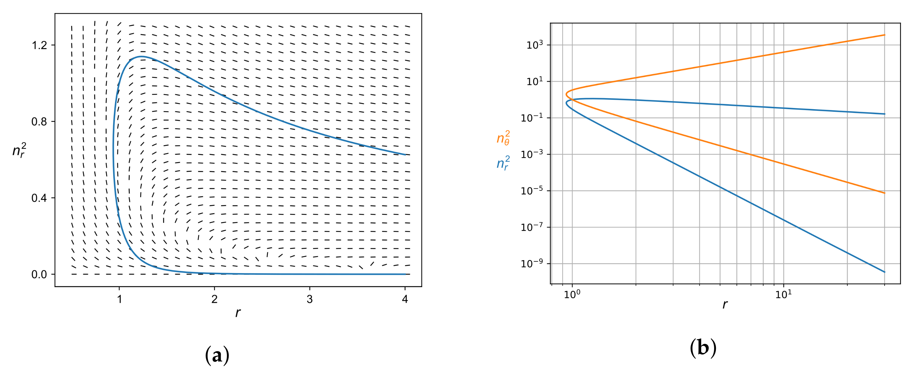
Thus, without loss of generality, we may, by rescaling any solution, take $k_{\theta }$ to be 0 or 1 and k to be $-1$, 0, or 1. If $k=0$, then there is essentially just one solution: $s_0\left(r\right)$ satisfying $s_0\left(1\right)=1$ with all other solutions (with $k_{\theta }=1$) taking the form $s\left(r\right)={\lambda }^2{s}_0\left(\lambda r\right)$, parametrized by $\lambda$. The solutions for $s_0\left(r\right)=n_r^2\left(r\right)$ and $n_{\theta }^2\left(r\right)=1/\left(r^4{n}_r^2\right)$ are shown in Figure 2 along with the flow field. One can see that the solution does not exist below a critical value of r, which looks unsatisfactory. This critical radius is associated with the vanishing of the denominator in (80).

To obtain satisfactory solutions that exist for all $r\ne 0$, one may take $k_{\theta }=0$ and $k=1$ to avoid the denominator in (80) vanishing, except at $r=0$. Then, (80) reduces to

$$\frac{ds}{dr}=-\frac{2s(r^2{s}^2+2)}{r(3r^2{s}^2+k)},\mathrm{where}s=n_r^2.$$

(82)

There is again essentially just one solution: $s_0\left(r\right)$ satisfying $s_0\left(1\right)=1$ with all other solutions (with $k=1$) taking the form $s\left(r\right)=\lambda s_0\left(\lambda r\right)$, parametrized by $\lambda$. The solution is graphed in Figure 3. There is a singularity at $r=0$, and while $n_r^2\left(r\right)$ goes rapidly to zero as $r\to \infty$, $n_4^2\left(r\right)$ and $n_z^2\left(r\right)$ (unless it is zero) diverge to ∞ as $r\to \infty$. This solution is satisfactory once one takes into account that the weak field approximation is not valid near the singularity at $r=0$, nor as $r\to \infty$, and one should use the full equations (37) there. For this example with $k=1$ and $k_{\theta }=0$, it is interesting that there is a transition from a superluminal region inside to a subluminal region outside according to the sign of

$$n^2-n_4^2=n_r^2+\frac{k_z^2}{r^2{n}_r^2}-\frac{k_4^2}{r^2{n}_r^2}=n_r^2-\frac{1}{r^2{n}_r^2},$$

(83)

which is also plotted in Figure 3.

9. Extension of the Schwarzschild Solutions with Spherical Symmetry

Here, we generalize Schwarzschild’s solution for a spherically symmetric metric solving Einstein’s equations in the absence of matter. The important point is that in appropriate limits, some of the solutions here approach the Schwarzschild solution. Consequently, existing experimental results of black holes do not invalidate our theory, but rather place constraints on the magnitude of the torsion field. This magnitude should be tied to the radius of the universe, and, hence, to the critical acceleration in MOND. Thus, experiments in the near vicinity of a star or black hole would not typically reveal the difference with Schwarzschild’s solution. We have not explored the situation regarding rotating black holes.

As shown by Schwarzschild, the metric in “polar” coordinates spherically symmetric about the origin must be of the form

$$d{s}^2=ad{r}^2+r^2(d{\theta }^2+{sin}^2\theta d{\varphi }^2)-bd{t}^2,$$

(84)

in which a and b are functions of r and t. Here, we look for solutions where they are functions of r only. Setting $x_1=r$, $x_2=\theta$, $x_3=\varphi$, $x_4=t$ allows us to use (84) to identify the coefficients:

$$g_{11}=a,g_{22}=r^2,g_{33}=r^2{sin}^2\theta ,g_{44}=-b.$$

(85)

From (36), we obtain the ten equations:

$$\begin{array}{ccc}\hfill 0& =& {\overline{R}}_{11}=\frac{a^{\prime }}{ar}+\frac{a^{\prime }{b}^{\prime }}{4ab}+\frac{{\left(b^{\prime }\right)}^2}{4b^2}-\frac{b^{″}}{2b}+2a[r^2{\left(N^2\right)}^2+r^2{sin}^2\theta {\left(N^3\right)}^2-b{\left(N^4\right)}^2],\hfill \\ \hfill 0& =& {\overline{R}}_{22}=1-\frac{1}{a}+\frac{r{a}^{\prime }}{2a^2}-\frac{r{b}^{\prime }}{2ab}+2r^2[a{\left(N^1\right)}^2+r^2{sin}^2\theta {\left(N^3\right)}^2-b{\left(N^4\right)}^2],\hfill \\ \hfill 0& =& {\overline{R}}_{33}=[1-\frac{1}{a}+\frac{r{a}^{\prime }}{2a^2}-\frac{r{b}^{\prime }}{2ab}]{sin}^2\theta +2r^2{sin}^2\theta [a{\left(N^1\right)}^2+r^2{\left(N^2\right)}^2-b\left(N^4\right)],\hfill \\ \hfill 0& =& {\overline{R}}_{44}=\left(\frac{b^{\prime }}{ar}+\frac{b^{″}}{2a}-\frac{{\left(b^{\prime }\right)}^2}{4ab}-\frac{a^{\prime }{b}^{\prime }}{4a^2}\right)-2b[a{\left(N^1\right)}^2+r^2{\left(N^2\right)}^2+r^2{sin}^2\theta {\left(N^3\right)}^2],\hfill \\ \hfill 0& =& {\overline{R}}_{mn}=-2g_{mm}{g}_{nn}{N}^m{N}^n\mathrm{for}\mathrm{all}m,n\mathrm{with}m\ne n,\mathrm{no}\mathrm{sum}\mathrm{on}m,n,\hfill \end{array}$$

(86)

where the terms not involving $\mathbf{N}$ can be identified with the standard formulas for the elements $R_{ij}^0$ that are zero when $i\ne j$. Here, differentiation with respect to $x_1=r$ is denoted by the prime, with the double prime denoting the second derivative. The second and third equations and the last equation force $N^2=N^3=0$, which is not surprising considering the symmetry of the problem. Two possibilities remain: either $N^1=0$ or $N^4=0$. The first case corresponds to a subluminal solution and the second to a superluminal solution.

Let us consider first the case where $N^1=N^2=N^3=0$. Multiplying the second last equation in (86) by $a/b$ and adding it to the first gives

$$\frac{a^{\prime }}{a}+\frac{b^{\prime }}{b}-2q=0\mathrm{where}q=rab{\left(N^4\right)}^2\ge 0.$$

(87)

The second equation in (86) implies

$$\frac{a^{\prime }}{a}-\frac{b^{\prime }}{b}+2(a-1)/r-4q=0.$$

(88)

Adding and subtracting these equations gives

$$\begin{array}{ccc}\hfill a^{\prime }/a& =& \frac{1}{r}-\frac{a}{r}+3q,\hfill \\ \hfill b^{\prime }/b& =& \frac{a}{r}-\frac{1}{r}-q.\hfill \end{array}$$

(89)

Multiplying the last by $br$, differentiating it, and using the result to eliminate $b^{″}$ from the first equation in (86) yield

$$q^{\prime }=2q^2+\frac{q}{r}.$$

(90)

This has the solution

$$q=\frac{{\alpha }^{2}r}{1-{\alpha }^2{r}^2},$$

(91)

where $\alpha$ is a constant. Furthermore, by replacing q with $rab{\left(N^4\right)}^2$, one obtains

$$\begin{array}{ccc}\hfill 2q^2+\frac{q}{r}=q^{\prime }& =& ab{\left(N^4\right)}^2+(r{a}^{\prime }/a)ab{\left(N^4\right)}^2+(r{b}^{\prime }/b)ab{\left(N^4\right)}^2+rab\frac{d{\left(N^4\right)}^2}{dr},\hfill \\ & =& \frac{q}{r}[1+(1-a+3qr)+(a-1-qr)]+q\frac{d{\left(N^4\right)}^2}{dr}=\frac{q}{r}+2q^2+q\frac{d{\left(N^4\right)}^2}{dr}.\hfill \end{array}$$

(92)

This implies that ${\left(N^4\right)}^2$ is a constant that we call ${\beta }^2$, giving

$$\frac{a}{r}=\frac{q}{b{r}^2{\left(N^4\right)}^2}=\frac{{\alpha }^2}{br{\beta }^2(1-{\alpha }^2{r}^2)}.$$

(93)

Substituting this back in the second equation in (89) gives the linear first-order differential equation:

$$\frac{db}{dr}+b\left[\frac{1}{r}+\frac{{\alpha }^2}{1-{\alpha }^2{r}^2}\right]=\frac{{\alpha }^2}{{\beta }^{2}r(1-{\alpha }^2{r}^2)}.$$

(94)

Multiplying both sides by the integrating factor of $r/\sqrt{1-{\alpha }^2{r}^2}$ gives

$$\frac{d}{dr}\left[br/\sqrt{1-{\alpha }^2{r}^2}\right]=\frac{{\alpha }^2}{{\beta }^2(1-{\alpha }^2{r}^2)\sqrt{1-{\alpha }^2{r}^2}}.$$

(95)

Integrating both sides and recalling (93), we obtain

$$\begin{array}{ccc}\hfill b& =& \frac{{\alpha }^2}{{\beta }^2}-2m\frac{\sqrt{1-{\alpha }^2{r}^2}}{r},\hfill \\ \hfill a& =& \frac{{\alpha }^2}{b{\beta }^2(1-{\alpha }^2{r}^2)},\hfill \end{array}$$

(96)

where m is a constant of integration. In particular, with ${\alpha }^2={\beta }^2$, this becomes

$$\begin{array}{ccc}\hfill b& =& 1-2m\frac{\sqrt{1-{\alpha }^2{r}^2}}{r},\hfill \\ \hfill a& =& \frac{1}{b(1-{\alpha }^2{r}^2)},\hfill \end{array}$$

(97)

which in the limit $\alpha \to 0$ reduces to the familiar Schwarzschild solution:

$$a=\frac{1}{1-2m/r},b=1-2m/r,$$

(98)

which becomes Euclidean at large r. Once we allow nonzero $\alpha$, the space is no longer Euclidean at large r, but it still has a black hole at the center, with a diverging when $r=2m\sqrt{1-{\alpha }^2{r}^2}$ and at $r=1/{\alpha }^2$, the latter corresponding to the closed universe studied in the next section.

Now, consider the second possibility that $N^2=N^3=N^4=0$. Again, multiplying the second last equation in (86) by $a/\left(b\right)$ and adding it to the first give

$$\frac{a^{\prime }}{a}+\frac{b^{\prime }}{b}-2w=0\mathrm{where}w=r{a}^2{\left(N^1\right)}^2\ge 0.$$

(99)

Furthermore, the second equation in (86) implies

$$\frac{a^{\prime }}{a}+\frac{b^{\prime }}{b}+2(a-1)/r+4w=0.$$

(100)

Adding and subtracting these equations give

$$\begin{array}{ccc}\hfill a^{\prime }/a& =& \frac{1}{r}-\frac{a}{r}-w,\hfill \\ \hfill b^{\prime }/b& =& \frac{a}{r}-\frac{1}{r}+3w.\hfill \end{array}$$

(101)

Multiplying the last by $br$, differentiating it, and using the result to eliminate $b^{″}$ from the first equation in (86) yield

$$w^{\prime }=-2w^2+w(1-\frac{4}{3}a)/r.$$

(102)

The equations (101) and (102) appear to have no simple analytic solution. One may eliminate $a\left(r\right)$ from the two equations that do not involve $b\left(r\right)$ to obtain

$$\frac{w^{″}}{w}=\frac{7{\left(w^{\prime }\right)}^2}{4w^2}-\frac{3w^{\prime }}{2wr}-\frac{2w}{r}+w^2-\frac{1}{4r^2},$$

(103)

and from a solution $w\left(r\right)$, (102) easily gives $a\left(r\right)$. Alternatively, one may eliminate $w\left(r\right)$ from these equations to obtain

$$\frac{v^{″}}{v}=\frac{3{\left(v^{\prime }\right)}^2}{v^2}+\frac{v^{\prime }}{vr}+(5v^{\prime }+2v^2)/3+v/r.$$

(104)

where $v=a/r$, and given a solution $a\left(r\right)=rv\left(r\right)$, the first equation in (101) yields $w\left(r\right)$. In either case, $b\left(r\right)$ is found by integrating the last equation in (101). Note that if $b\left(r\right)$ is a solution, then so will be ${\lambda }^{2}b\left(r\right)$ for any constant $\lambda$, i.e., $b\left(r\right)$ is only determined up to a multiplicative constant. This reflects the fact that we are free to rescale the time coordinate, replacing t by $t/\lambda$ in (84).

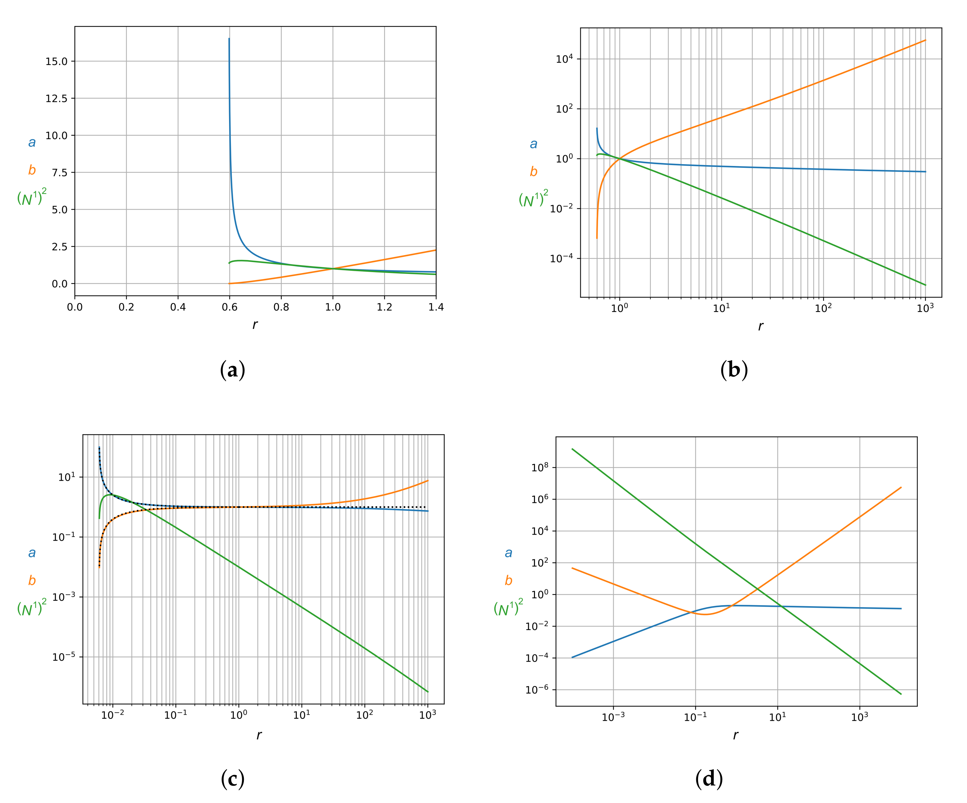
Rather than dealing with these second-order equations for $w\left(r\right)$ and $v\left(r\right)$, one can numerically solve (101) and (102) directly. Figure 4 shows some typical solutions, excluding unphysical examples where, say, $a\left(r\right)$ or $w\left(r\right)$ remain negative for all r.

10. Homogeneous Expanding Universe

It should be emphasized that the solution given here, which is incompatible with the observations, is for a homogeneous universe devoid of ordinary matter. It does not apply to a universe where spacetime itself has fluctuations that are not due to ordinary matter. Even ignoring ordinary gravitational effects, the perturbation results at the beginning of Section 8 imply such fluctuations occur, and so, one should expect that its cosmological predictions deviate from those presented in this section. This is explained further in the next section.

We take the Friedmann–Lemaître–Robertson–Walker metric in reduced-circumference polar coordinates:

$$d{s}^2=a^2\left[\frac{d{r}^2}{1-k{r}^2}+r^2(d{\theta }^2+{sin}^2\theta d{\varphi }^2)\right]-d{t}^2$$

(105)

where a, the reduced circumference, can be a function of time, while r, $\theta$, and $\varphi$ are time independent, and $k=1,0,-1$, according to whether the universe is spatially closed, flat, or open with negative curvature. With $x_1=r$, $x_2=\theta$, $x_3=\varphi$, and $x_4=t$, the corresponding metric coefficients are

$$g_{11}=a^2/(1-k{r}^2),g_{22}=a^2{r}^2,g_{33}=a^2{r}^2{sin}^2\theta ,g_{44}=-1.$$

(106)

Assuming $N^1=N^2=N^3=0$ and defining

$$P=2k+(a\ddot{a}+2{\dot{a}}^2),$$

(107)

where the dot and double dot denote first and second derivatives with respect to time, the equations become

$$\begin{array}{ccc}\hfill 0& =& {\overline{R}}_{11}=-2{\left(N^4\right)}^2{a}^2/(1-k{r}^2)-P/(1-k{r}^2),\hfill \\ \hfill 0& =& {\overline{R}}_{22}=-2{\left(N^4\right)}^2{a}^2{r}^2-P{r}^2,\hfill \\ \hfill 0& =& {\overline{R}}_{33}=-2{\left(N^4\right)}^2{a}^2{r}^2{sin}^2\theta -P{r}^2{sin}^2\theta ,\hfill \\ \hfill 0& =& {\overline{R}}_{44}=3\ddot{a}/a,\hfill \end{array}$$

(108)

where the terms not involving $N^4$ can be identified with the standard formulas for $R_{ij}^0$. The last equation in (108) implies $\dot{a}$ is a constant that we define to be $\beta$. We obtain

$$P=2k+2{\dot{a}}^2=2(k+{\beta }^2),a=\beta t+\gamma ,$$

(109)

where $\gamma$ is an integration constant that we can choose to be zero by redefining our origin of time appropriately (except in the trivial case of a spatially flat universe independent of time with $N_4=0$). From the remaining three equations in (107), which are all equivalent, we obtain

$${\left(N^4\right)}^2=-\frac{P}{2a^2}=-\frac{k+{\beta }^2}{{\beta }^2{t}^2},$$

(110)

which implies that $k=-1$ (an open universe, like in anti-de Sitter spacetime) and ${\beta }^2<1$.

11. Addressing the Dark Matter and Dark Energy Problem

The result of the previous section giving an expansion rate $\dot{a}$ independent of time agrees with the well-known result that $\ddot{a}=0$ for a model with $p=-{\mu }_0/3$. However, this is based on the premise that spacetime is homogeneous. The expansion of the universe appears to be accelerating with measurements indicating $p=-0.8{\mu }_0$ [8], and this could be a consequence of our theory, as we now explain.

Dark matter itself is known to be inhomogeneous; see, for example, [45] and the references therein. Spacetime is also inhomogeneous in our model. As the analysis at the beginning of Section 8 shows, if there is a small fluctuation in the torsion vector field in subluminal or superluminal regions of spacetime, then that perturbation will grow. Moreover, ordinary gravitational effects might add to the inhomogeneity: if there is a higher equivalent mass density in two different regions, then there could be gravitational attraction between these regions, leading to accretion. At the same time, “collisions” between accreting regions should tend to disperse the torsion vector field density. Thus, there will be a certain amount of equivalent kinetic energy associated with the torsion field accounting for some additional “dark energy”. More importantly, there could be substructures in the torsion field containing differing ratios of “dark energy” to “dark mass”. The structures could collide and give rise to different structures. In particular, there might be “negative mass structures”, by which we mean structures in the torsion vector field incorporating superluminal regions. Accounting for these effects should reduce the total mass density, providing a higher $p/{\mu }_0$ ratio, which may be consistent with the experimental value of $-0.8$.

It is to be emphasized that both our full equations (37) and their weak field approximations (46), (47), and (57) have no intrinsic length scale. There is a length scale associated with the overall density of the torsion vector field (connected with the mass density of the apparent dark matter and dark energy in our theory), but this is of the order of the radius of the universe. It seems likely that the torsion vector field could be quite turbulent with structures on many length scales, down to some lower cutoff length scale where the current theory breaks down. This cutoff could be the Planck length scale.

To provide quantitative predictions, one needs a better idea of the behavior of the torsion vector field within spacetime, and this will almost certainly require sophisticated numerical simulations to obtain an approximation to the “macroscopic equation of state”. Simulations are needed to provide a better understanding of torsion fluid behavior in intergalactic and interstellar regions, as well as around stars, globular clusters, galaxies, and galaxy clusters. These may require the introduction of some parameter that provides a lower length scale to the “turbulence” in the torsion vector field, which ultimately could be taken to be very small. Simulating the dynamics of the torsion vector field over the continuum of length scales may also require a sort of numerical renormalization group approach. While we have not investigated the stability of the torsion waves and torsion-rolls, it is not important that they are stable, even in the weak field approximation. The purpose of our exact solutions in the weak field approximation was mainly to illustrate the rich dynamics of the torsion vector field, to give some insight into possible dynamics and to show that one can have transitions between subluminal and superluminal regions, as noted at the end of Section 8.2.

Regarding the question as to whether our model can account for the galactic dark mass problem, an encouraging sign is the apparent cosmological connection between the critical acceleration $a_0\approx 1.2\times {10}^{-10}{\mathrm{m}/\mathrm{s}}^2$ in MOND, the radius of the universe, and the density of dark matter or energy in the universe, as reviewed in [46]. Thus, the density of dark matter or energy, roughly $\varrho \approx {10}^{-27}{\mathrm{kg}/\mathrm{m}}^3$, which in our theory is related to the strength of the torsion field $\mathbf{N}$, has an associated length scale $1/\sqrt{c^2\varrho \kappa }\approx 6\times {10}^{26}$ meters (approximately the radius of the universe), which agrees with the length scale $c^2/a_0\approx 7.5\times {10}^{26}$ meters associated with the critical acceleration $a_0$ in MOND.

12. Discussion

The theory presented here is largely aimed at providing equations governing the behavior of spacetime and the torsion field in regions devoid of matter. An initial test of the theory would entail numerical simulations of the torsion field in the weak field approximation with ordinary gravitational effects neglected, as governed by Equation (57), and allowing for field fluctuations. These fluctuations in the torsion field should be truncated at a small length scale, perhaps at the Planck length scale. This should give an approximation to the effective equation of state. The next step would be to determine the evolution of a homogeneous closed universe with this equation of state. Then, perturbations could be introduced and the evolution studied. For the theory to be viable, without modification, the results need to be consistent with cosmological observations.

Beyond the need for a lower cutoff, the equations are still incomplete. As remarked already, one can change the sign of $\mathbf{N}\left(\mathbf{x}\right)$ in any region and still satisfy the equations, indicating that there is a deeper theory that prevents such discontinuous solutions for $\mathbf{N}\left(\mathbf{x}\right)$. Perhaps this also enters at the Planck length scale, and both it and the truncation of fluctuations in the torsion field are accounted for by appropriate quantum equations. Assuming there is only weak coupling between the torsion fluid with matter, aside from the coupling due to gravitation (spacetime curvature), then one might think there is conservation of momentum and energy both for the stress–energy–momentum tensor of the torsion vector field and for the stress–energy–momentum tensor of matter. On the other hand, if one regards the conservation of momentum and energy as a consequence of the Bianchi identities, then there appears to be no reason why they should be separately conserved. For this reason, our current theory, while it describes the curvature of spacetime and the accompanying torsion vector field in regions devoid of matter, is incomplete in regions containing matter.

One appealing feature of Cartan’s equations, and which is absent in our current theory, is that they allow for the incorporation of intrinsic spin—something that was discovered in 1925–1926 after Cartan first arrived at his remarkable equations. Cartan was originally motivated by the work of the Cosserat brothers [47], who, like his equations, allowed for a non-symmetric stress field. His focus was on deriving equations where the source (matter) field automatically satisfied energy and momentum conservation. Sciama [48] and Kibble [49] independently developed the same generalization of Cartan’s theory, known as $U_4$ or the Einstein–Cartan–Sciama–Kibble theory. Their theory and the original Cartan theory imply that the torsion field is zero in empty space and, so, reduce to the Einstein equations when matter is not present. An advantage of these theories, not yet incorporated in our theory as there is no coupling with matter, is that they account for the conservation of angular momentum [30].

As others have also realized, departing from Cartan’s approach has the potential for explaining dark energy and dark matter as manifestations of a revised gravitational theory. Our theory is perhaps the simplest theory with that potential. As stressed already, conservation of energy and momentum still hold provided one reinterprets the equations as Einstein’s equation with an energy–momentum–stress tensor associated with “empty space”, i.e., associated with the torsion field. It could be that more complicated equations involving torsion will provide the final answer (and, as observed in the introduction, many candidates, besides Cartan’s and those of Sciama and Kibble, have been proposed, and undoubtedly, others will be put forward in the future). In that case, it could be that the ultimate theory only slightly perturbs the results in our theory in the intergalactic and interstellar regions, yet provides some lower limit to the likely “turbulence” in the torsion field. Thus, if successful, the theory proposed here may provide a guide in the search for the ultimate theory. It may be that the most important “take home” message of this paper is highlighting the importance of considering torsion theories that allow for dynamics in empty space on multiple length scales of the torsion field (and hence, of the accompanying metric). Interestingly, even in the absence of any torsion, anti-de Sitter space has a weakly turbulent instability [14].

If warranted by experimental observations, a natural modification of our theory would be to add a term involving Einstein’s cosmological constant $\Lambda$. However, it would be far more satisfying if this was not needed.

References

- Peebles, P.J.E.; Ratra, B. The cosmological constant and dark energy. Rev. Mod. Phys. 2003, 75, 559–606. [Google Scholar] [CrossRef] [Green Version]
- Sahni, V. Dark Matter and Dark Energy. In The Physics of the Early Universe; Lecture Notes in Physics; Springer: Berlin/Heidelberg, Germany; London, UK, 2004; Volume 653, Chapter 5; pp. 141–179. [Google Scholar] [CrossRef] [Green Version]
- Collin, R.E. Dynamics of Dark Energy. Int. J. Mod. Phys. D 2006, 15, 1753–1935. [Google Scholar] [CrossRef] [Green Version]
- Frieman, J.A.; Turner, M.S.; Huterer, D. Dark Energy and the Accelerating Universe. Annu. Rev. Astron. Astrophys. 2008, 46, 385–432. [Google Scholar] [CrossRef] [Green Version]
- Amendola, L.; Tsujikawa, S. Dark Energy: Theory and Observations; Cambridge University Press: Cambridge, UK, 2010; p. xiii. 491p. [Google Scholar] [CrossRef]
- Li, M.; Li, X.D.; Wang, S.; Wang, Y. Dark Energy. Commun. Theor. Phys. 2016, 56, 525–604. [Google Scholar] [CrossRef] [Green Version]
- Arun, K.; Gudennavar, S.B.; Sivaram, C. Dark matter, dark energy, and alternate models: A review. Adv. Space Res. 2017, 60, 166–186. [Google Scholar] [CrossRef] [Green Version]
- Abbott, T.; Abbott, T.M.C.; Alarcon, A.; Allam, S.; Andersen, P.; Andrade-Oliveira, F.; Annis, J.; Asorey, J.; Avila, S.; Bacon, D.; et al. Cosmological Constraints from Multiple Probes in the Dark Energy Survey. Phys. Rev. Lett. 2019, 122, 171301. [Google Scholar] [CrossRef] [Green Version]
- Nadler, E.O.; Drlica-Wagner, A.; Bechtol, K.; Mau, S.; Wechsler, R.H.; Gluscevic, V.; Boddy, K.; Pace, A.B.; Li, T.S.; McNanna, M. Milky Way Satellite Census. III. Constraints on Dark Matter Properties from Observations of Milky Way Satellite Galaxies. Phys. Rev. Lett. 2021, 126, 091101. [Google Scholar] [CrossRef]
- Wong, K.C.; Suyu, S.H.; Chen, G.C.; Rusu, C.E.; Millon, M.; Sluse, D.; Bonvin, V.; Fassnacht, C.D.; Taubenberger, S.; Auger, M.W. H0LiCOW XIII. A 2.4 per cent measurement of H0 from lensed quasars: 5.3σ tension between early and late-Universe probes. Mon. Not. R. Astron. Soc. 2020, 498, 1420–1439. [Google Scholar] [CrossRef]
- Riess, A.G.; Casertano, S.; Yuan, W.; Macri, L.M.; Scolnic, D. Large Magellanic Cloud Cepheid Standards Provide a 1% Foundation for the Determination of the Hubble Constant and Stronger Evidence for Physics beyond ΛCDM. Astrophys. J. 2019, 876, 85. [Google Scholar] [CrossRef]
- Chae, K.H.; Lelli, F.; Desmond, H.; McGaugh, S.S.; Li, P.; Schombert, J.M. Testing the Strong Equivalence Principle: Detection of the External Field Effect inRotationally Supported Galaxies. Astrophys. J. 2020, 904, 51. [Google Scholar] [CrossRef]
- Pigozzo, C.; Carneiro, S.; Alcaniz, J.; Borges, H.; Fabris, J. Evidence for cosmological particle creation? J. Cosmol. Astropart. Phys. 2016, 2016, 022. [Google Scholar] [CrossRef] [Green Version]
- Bizoń, P.; Rostworowski, A. Weakly Turbulent Instability of Anti-de Sitter Spacetime. Phys. Rev. Lett. 2011, 107, 031102. [Google Scholar] [CrossRef] [PubMed] [Green Version]
- Krasiński, A. Accelerating expansion or inhomogeneity? A comparison of the ΛCDM and Lemaître-Tolman models. Phys. Rev. D 2014, 89, 023520, Erratum in Phys. Rev. D 2014, 89, 089901. [Google Scholar] [CrossRef] [Green Version]
- Wang, B.; Abdalla, E.; Atrio-Barandela, F.; Pavón, D. Dark matter and dark energy interactions: Theoretical challenges, cosmological implications and observational signatures. Rep. Prog. Phys. 2016, 79, 096901. [Google Scholar] [CrossRef] [Green Version]
- Borges, H.A.; Wands, D. Growth of structure in interacting vacuum cosmologies. Phys. Rev. D 2020, 101, 103519. [Google Scholar] [CrossRef]
- Sabbata, V.D.; Sivaram, C. Spin and Torsion in Gravitation; World Scientific Publishing Co.: Singapore; Philadelphia, PA, USA; River Edge, NJ, USA, 1994; p. 328. [Google Scholar]
- Ray, S.; Khlopov, M.; Ghosh, P.P.; Mukhopadhyay, U. Phenomenology of ΛCDM model: A possibility of accelerating Universe with positive pressure. Int. J. Theor. Phys. 2011, 50, 939–951. [Google Scholar] [CrossRef] [Green Version]
- Famaey, B.; McGaugh, S.S. Modified Newtonian Dynamics (MOND): Observational Phenomenology and Relativistic Extensions. Living Rev. Relativ. 2012, 15, 10. [Google Scholar] [CrossRef] [Green Version]
- Milgrom, M. A modification of the Newtonian dynamics: Implications for galaxy systems. Astrophys. J. 1983, 270, 384–389. [Google Scholar] [CrossRef]
- Bekenstein, J.D. Relativistic gravitation theory for the modified Newtonian dynamics paradigm. Phys. Rev. D 2004, 70, 083509. [Google Scholar] [CrossRef]
- Skordis, C. Generalizing tensor-vector-scalar cosmology. Phys. Rev. D 2008, 77, 123502. [Google Scholar] [CrossRef] [Green Version]
- Merritt, D. A Philosophical Approach to MOND: Assessing the Milgromian Research Program in Cosmology; Cambridge University Press: Cambridge, UK, 2020; p. 285. [Google Scholar]
- Milgrom, M. MOND vs. dark matter in light of historical parallels. Stud. Hist. Philos. Sci. Part B Stud. Hist. Philos. Mod. Phys. 2020, 71, 170–195. [Google Scholar] [CrossRef] [Green Version]
- Frieman, J.A.; Turner, M.S.; Huterer, D. A unifying theory of dark energy and dark matter: Negative masses and matter creation within a modified ΛCDM framework. Astron. Astrophys. 2018, 620, A92. [Google Scholar] [CrossRef] [Green Version]
- Cartan, E. Sur les variétés à Connexion Affine et la théorie de la Relativit é Généralisée; Gauthier Villars: Paris, France, 1955. [Google Scholar]
- Magnon, A.; Ashtekar, A. On Manifolds with an Affine Connection and the Theory of General Relativity; Monographs and Textbooks in Physical Science (Book 1); Bibliopolis: Napoli, Italy, 1986; p. 199. [Google Scholar]
- Misner, C.W.; Thorne, K.S.; Wheeler, J.A. Gravitation, 3rd ed.; Freeman: San Francisco, CA, USA, 1973; p. xxvi. 1279p. [Google Scholar]
- Hehl, F.W.; von der Heyde, P.; Kerlick, G.D.; Nester, J.M. General Relativity with spin and torsion: Foundations and prospects. Rev. Mod. Phys. 1976, 48, 393–416. [Google Scholar] [CrossRef] [Green Version]
- Hehl, F.W.; McCrea, J.D.; Mielke, E.W.; Ne’eman, Y. Metric-affine gauge theory of gravity: Field equations, Noether identities, world spinors, and breaking of dilation invariance. Phys. Rep. 1995, 258, 1–171. [Google Scholar] [CrossRef] [Green Version]
- Shapiro, I. Physical aspects of the space–time torsion. Phys. Rep. 2002, 357, 113–214. [Google Scholar] [CrossRef] [Green Version]
- Ortín, T. Gravity and Strings; Cambridge Monographs on Mathematical Physics: Cambridge, UK, 2004; p. xx. 684p. [Google Scholar] [CrossRef]
- Trautman, A. Einstein–Cartan Theory; Encyclopedia of Mathematical Physics; Elsevier: Amsterdam, The Netherlands, 2006; Volume 2, pp. 189–195. [Google Scholar]
- Popławski, N.J. Spacetime and fields. arXiv 2009, arXiv:0911.0334. [Google Scholar]
- Fabbri, L. Fundamental Theory of Torsion Gravity. Universe 2021, 7, 305. [Google Scholar] [CrossRef]
- Jiméneza, J.B.; Heisenberg, L.; Koivisto, T.S. The Geometrical Trinity of Gravity. Universe 2019, 5, 173. [Google Scholar] [CrossRef] [Green Version]
- Ivanov, A.N.; Wellenzohn, M. Einstein–Cartan Gravity with Torsion Field Serving as Origin for Cosmological Constant or Dark Energy Density. Astrophys. J. 2016, 829, 47. [Google Scholar] [CrossRef]
- Sengupta, S. Gravity theory with a dark extra dimension. Phys. Rev. D 2020, 101, 104040. [Google Scholar] [CrossRef]
- Watanabe, T.; Hayashi, M.J. General relativity with torsion. arXiv 2004, arXiv:gr-qc/0409029. [Google Scholar]
- Minkevich, A.V. Accelerating Universe with spacetime torsion but without dark matter and dark energy. Phys. Lett. B 2009, 678, 423–426. [Google Scholar] [CrossRef] [Green Version]
- De Berredo-Peixoto, G.; de Freitas, E.A. On the torsion effects of a relativistic spin fluid in early cosmology. Class. Quantum Gravity 2009, 26, 175015. [Google Scholar] [CrossRef]
- Belyaev, A.S.; Thomas, M.C.; Shapiro, I.L. Torsion as a Dark Matter Candidate from the Higgs Portal. Phys. Rev. D 2017, 95, 095033. [Google Scholar] [CrossRef] [Green Version]
- Vasak, D.; Kirsch, J.; Struckmeier, J. Dark energy and inflation invoked in CCGG by locally contorted spacetime. Eur. Phys. J. Plus 2020, 135, 404. [Google Scholar] [CrossRef]
- Nierenberg, A.M.; Gilman, D.; Treu, T.; Brammer, G.; Birrer, S.; Moustakas, L.; Agnello, A.; Anguita, T.; Fassnacht, C.D.; Motta, V.; et al. Double dark matter vision: Twice the number of compact-source lenses with narrow-line lensing and the WFC3 grism. Mon. Not. R. Astron. Soc. 2019, 492, 5314–5335. [Google Scholar] [CrossRef] [Green Version]
- Milgrom, M. The a0–cosmology connection in MOND. arXiv 2009, arXiv:2001.09729. [Google Scholar]
- Cosserat, E.M.P.; Cosserat, F. Theory of Deformable Bodies; NASA: Washington, DC, USA, 1968; p. vi. 220p.
- Sciama, D.W. The analogy between charge and spin in general relativity. In Recent Developments in General Relativity; Festschrift for Leopold Infeld; Państwowe Wydawnictwo Naukowe: Warsaw, Poland; Pergamon Press: New York, NY, USA, 1962; pp. 415–439. [Google Scholar]
- Kibble, T.W.B. Lorentz invariance and the gravitational field. J. Math. Phys. 1961, 2, 212–221. [Google Scholar] [CrossRef] [Green Version]
Figure 1.
Figure, courtesy of M. Milgrom, taken from http://www.scholarpedia.org/article/The_MOND_paradigm_of_modified_dynamics, (accessed on 31 March 2020) showing its predictions, which are consistent with experimental observations. Plotted is the acceleration as a function of the distance from an isolated mass M, for a star with (red), a globular cluster with (blue), a galaxy with (green), and a galaxy cluster with (magenta), in which represents one solar mass.
Figure 2.
Solution for the torsion field with cylindrical symmetry with , , and . (a) The flow field when and and the particular solution satisfying when . (b) The same solution for on a log–log plot and the accompanying function .
Figure 3.
Solution for the torsion field with cylindrical symmetry with , , and . (a) The graph of showing its divergence as . (b) The plot of showing a transition from superluminal to subluminal as r increases.
Figure 4.
Numerical solutions of Equations (101) and (102). (a) Graph with showing a “black hole”-type singularity at . (b) Same as for (a), but on a log–log plot. Note the blow up of as . (c) Graph with and . Comparing this with (b) and taking note of the different vertical scales, one can see the approach to the usual Schwarzschild solution as . (d) Graph with , , and showing a different type of solution with no critical “black hole” radius, but rather, a singularity at . The solution for still clearly blows up as .
Publisher’s Note: MDPI stays neutral with regard to jurisdictional claims in published maps and institutional affiliations. |
© 2022 by the author. Licensee MDPI, Basel, Switzerland. This article is an open access article distributed under the terms and conditions of the Creative Commons Attribution (CC BY) license (https://creativecommons.org/licenses/by/4.0/).
Share and Cite
MDPI and ACS Style
Milton, G.W. A Possible Explanation of Dark Matter and Dark Energy Involving a Vector Torsion Field. Universe 2022, 8, 298. https://doi.org/10.3390/universe8060298
AMA Style
Milton GW. A Possible Explanation of Dark Matter and Dark Energy Involving a Vector Torsion Field. Universe. 2022; 8(6):298. https://doi.org/10.3390/universe8060298
Chicago/Turabian StyleMilton, Graeme W. 2022. "A Possible Explanation of Dark Matter and Dark Energy Involving a Vector Torsion Field" Universe 8, no. 6: 298. https://doi.org/10.3390/universe8060298
Note that from the first issue of 2016, this journal uses article numbers instead of page numbers. See further details here.