
Trajectory Analysis and Optimization of Hesperides Mission


Department of Civil and Industrial Engineering, University of Pisa, I-56122 Pisa, Italy
*
Author to whom correspondence should be addressed.
†
These authors contributed equally to this work.
Universe 2022, 8(7), 364; https://doi.org/10.3390/universe8070364
Submission received: 18 June 2022
/
Revised: 28 June 2022
/
Accepted: 29 June 2022
/
Published: 1 July 2022
(This article belongs to the Special Issue Exploration of Interstellar Space: Concepts, Space Science and Missions)
Abstract
:A challenging problem from a technological viewpoint is to send a spacecraft at a distance of about 600 au from the Sun, comparable with that of the Sun’s gravitational focus (that is, the general relativistic focusing of light rays, whose minimum solar distance is obtained when the light rays are assumed to graze the Sun’s surface), and reach it in a time interval on the order of a human working lifetime. A suitably oriented telescope at that distance would be theoretically able to observe exoplanets tens of light years far away and possibly to discover new life forms. The transfer trajectory of this mission is rather complex and requires a close selection of a suitable propulsion system, which must be able to provide the probe with the necessary energy to cruise at a velocity greater than 10 au/year. An effective outline of the these concepts is given by the Hesperides mission, originally proposed by Matloff in 2014. An interesting aspect of this mission proposal is the combination of a nuclear electric propulsion system and a classical solar sail that are jointly exploited to reach the necessary solar system escape velocity. However, the trajectory analysis reported by Matloff is very simplified and is essentially concentrated on a rough estimate of the time required by the spacecraft to reach a distance of 600 au. Starting from the Hesperides baseline mission proposal, including the vehicle mass distribution, the aim of this work is to give a detailed mission analysis in an optimal framework. In particular, the spacecraft minimum time trajectory is calculated with indirect methods and a parametric analysis is made to highlight the impact of the main design parameters on the total flight time. The simulations show a substantial reduction of the mission time when compared with the original study.
1. Introduction
Reaching the boundaries and escaping from the solar system within a time interval on the order of the human working lifetime is currently one of the most complex space mission scenarios from a trajectory analysis viewpoint [1]. Such a fascinating and advanced mission would be of great scientific interest to obtain information and solve fundamental physical questions about the formation mechanism of the heliospheric boundary, the nature of the nearby interstellar medium [2], the structure and dynamics of the heliosphere, and the distribution of matter in this part of interplanetary space [3]. Many, if not all, of these issues can only be solved through in situ measurements such as plasma density, ionization state, dust composition and magnetic field strength [4]. However, missions towards (and even beyond) the heliopause region represent a technological challenge [5], as they require the use of advanced propulsion systems [6] to guarantee a cruise velocity of at least 10 au/year if the spacecraft has to be able to reach the desired (very long) distance, greater than 100 au, in a reasonable time interval.
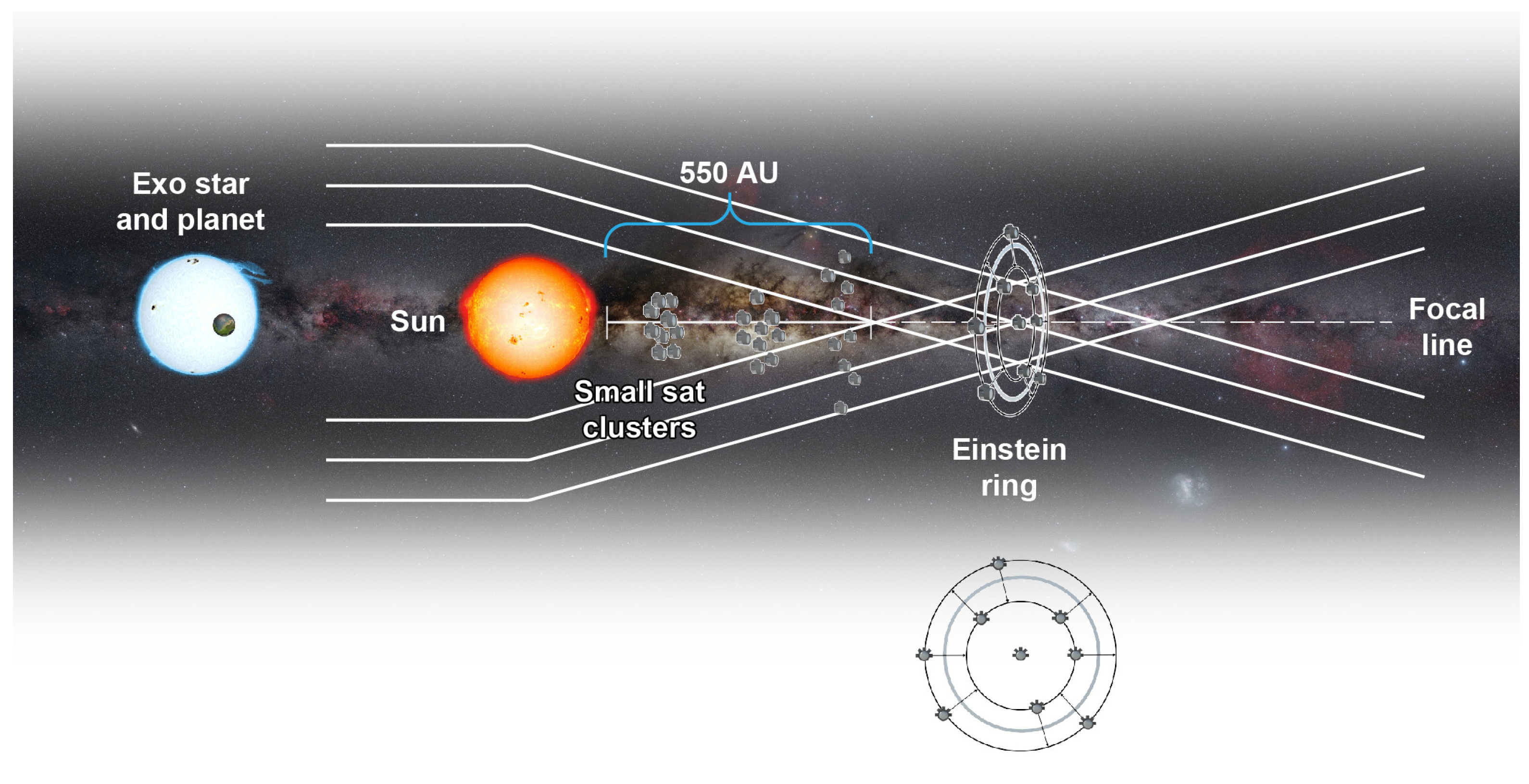
An even more futuristic and hard to manage project from a technological side is the dream to arrive at the Sun’s gravitational focus (SGF). According to general relativity theory, a massive object such as the Sun is able to deflect the light beams passing around it and to converge them at a focus. This effect implies that the Sun might be used as a sort of gravitational lens. However, differently from what happens in classical optics where the lens focus coincides with a single point, the gravitational effect causes the light beams passing at different distances from the Sun’s surface to converge at different points aligned along a straight line, which theoretically extends from about 550 au to the interstellar space (infinity), see Figure 1.
A light sensor placed at the focal region could therefore obtain images of exoplanets, some tens of light years far away, with a surface resolution of about 10 km for an Earth-like planet [7]. Note, however, that such a scenario requires staring almost at the Sun, with evident limitations for practical astronomy. This concept, first proposed by Eshleman [8] in 1979, has much attracted the attention of the scientific community, with many proposals for possible (and exotic) future missions [9,10,11]. A number of advances that could be obtained from a robotic mission to the SGF are in depth discussed by Maccone [12]. Such a fascinating mission concept may also be thought of as a necessary first step toward a future interstellar mission [13,14]. Even though a number of technical difficulties exist in translating the original idea into feasible achievements, including severe problems related to the telescope pointing requirements, the signal to noise ratio due to the solar corona and the focal blur [15], new studies on advanced missions to SGF continue to appear [16,17].
A possible way to address these complex problems is to decrease the mass of the scientific probe to be launched by distributing the whole payload among a fleet of smaller spacecraft, which could be deployed along an Einstein ring as illustrated in Figure 2. Among other advantages, a vehicle mass reduction implies higher spacecraft accelerations (assuming the thrust magnitude is unchanged) as well as increased escape velocities.
The enormous distances to reach during a (very long) space journey to the SGF make the transfer trajectory a very challenging task to plan, and so is the selection of a suitable propulsion system, capable of providing the required demanding and, more in general, the design of a space vehicle that must effectively operate along flight times of some tens of years [17]. An effective outline of the above ideas is offered by the Hesperides mission proposal [18], originally suggested by Matloff in 2014 as an evolution of a previous Helios and Prometheus concept, which dates back to 2007 [19]. The main aim of Hesperides mission is to reach a distance of about 600 au from the Sun, comparable with that of the SGF, within approximately five decades. An interesting aspect of the Hesperides mission is the combination of a nuclear electric propulsion system and a solar sail that are jointly exploited to reach the required solar system escape velocity. However the trajectory analysis reported in [18] is very simplified and is essentially concentrated on obtaining a rough estimate of the main design parameters necessary to meet the mission requirements, that is, mission times and final distances.
The aim of this paper is to revisit the Hesperides mission concept and to analyze it in an optimal and parametric way, by obtaining a more accurate estimate of both the (optimal) transfer trajectory and the flight times. It will be shown that a substantial performance improvement with respect to the original study [18] is a feasible result.
2. Spacecraft Characteristics and Baseline Mission Description
For illustrative purposes, the spacecraft arrangement and the baseline mission concept are taken from the original Hesperides proposal [18]. In particular, the solar sail is approximated as a thin disc with a radius of 146 m and a mass-to-area ratio equal to 0.003 kg/m2. The electric propulsion system uses xenon propellant exhausted at a constant mass flow rate and its specific impulse is . An estimate of the masses of the main spacecraft subsystems is reported in Table 1 and is illustrated in the pie chart of Figure 3.
The baseline mission [18] may be divided into the following four main phases:
- Pre-perihelion phase. The spacecraft is launched from Earth toward an heliocentric orbit with perihelion distance and aphelion distance . The required initial hyperbolic excess velocity is provided by an upper stage of the launcher, and the spacecraft reaches the target orbit with a flight time of about 2 years without using the solar sail or the electric thruster. In particular, the spacecraft mass in this phase is constant and equal to 450 kg.
- Solar sail acceleration. When the spacecraft is at the perihelion of the heliocentric orbit (end of phase 1) the solar sail is unfurled with a Sun-facing attitude [20,21,22,23], that is, its nominal plane is oriented normal to the Sun. In this phase, the spacecraft is continuously accelerated by the solar sail induced thrust until it reaches a solar distance of 5 au, when the sail propulsive acceleration becomes ineffective and is therefore jettisoned. During this whole phase, the spacecraft mass remains equal to 450 kg. The flight time of this phase is about 1 year.
- Radioisotope-electric propulsion. This phase starts when the solar sail is discarded, so that the spacecraft mass suddenly reduces to 249 kg. The radioisotope-electric thruster is switched on and is continuously operated until the whole available xenon propellant is exhausted at a constant mass flow rate . Since the total propellant mass is 100 kg, the phase (time) length is 10 years. During this phase the induced thrust is nearly along the radial direction, so that the spacecraft (heliocentric) hyperbolic excess velocity increases from about 35.5 km/s to 56 km/s, at a distance of about 100 au away from the Sun. At the end of this phase, the spacecraft mass is reduced to 149 kg.
- Cruise to 600 au. The last (baseline) trajectory part is a coasting phase with a constant velocity (with respect the Sun), equal to that reached at the end of phase 3. The spacecraft continues its (Keplerian) flight for about 42.5 years until it reaches a target distance of 600 au from the Sun. The spacecraft mass in this phase is constant and equal to 149 kg.
Accordingly, the total mission length is the sum of the flight times required to complete the previous four phases, that is, . Figure 4 summarizes the spacecraft mass variation during the four phases and the mission flight times.
3. Mission Optimization
The baseline mission is now reassessed within an optimal framework with the aim of investigating to what extent it may be improved. To that end, according to [18], a simplified two-dimensional model is used to describe the heliocentric spacecraft dynamics. More precisely, introduce a (heliocentric) polar reference frame , where O is the Sun’s center of mass, with orthogonal radial and transverse unit vectors and , respectively; see Figure 5. In this reference frame, the polar angle is measured counterclockwise from the Sun-spacecraft line at time .
The spacecraft equations of motion in may be written as
where r is the distance from the Sun, is the Sun’s gravitational parameter, u and v are the radial and transverse component of the spacecraft velocity, while and are the radial and transverse component of the spacecraft propulsive acceleration vector .
When the spacecraft is propelled by the solar sail, the propulsive acceleration components are
where is the spacecraft characteristic acceleration, that is, the acceleration magnitude induced by the solar sail when its nominal plane is perpendicular to the Sun-spacecraft line at a distance , and is the sail pitch angle measured counterclockwise from the Sun-spacecraft line; see Figure 5. The solar sail is here described through an augmented ideal force model [24,25] without degradation [26,27,28] or wrinkles [29]. In this context, the sail is assumed to maintain a flat surface, and the direction of the propulsive acceleration vector is normal to the sail nominal plane in the direction opposite to the Sun. The non-complete reflectivity of the sail film [30] is modeled by introducing a sort of sail efficiency factor , which quantifies the amount of reflected rays when compared to an ideal (specular) reflection case. Accordingly, the spacecraft characteristic acceleration may be written as
where is the solar radiation pressure at , 66,966 is the sail area and m is the spacecraft mass. In the simulations it has been assumed [18] that . With the aid of Equation (7) and using the data of Table 1, the spacecraft characteristic acceleration is therefore .
When the spacecraft is propelled by the electric thruster, the propulsive acceleration vector components are instead written as
where is the standard gravitational acceleration, and is the classical thrust angle measured counterclockwise from the radial direction. The spacecraft mass variation with time is therefore
For comparative purposes, the mission has been divided into the same phases as the baseline proposal, and each phase has been individually optimized using an indirect approach. Details about the optimization method may be found in previous works by the authors [31,32,33]. In particular, the spacecraft equations of motion have been numerically integrated using a variable order Adams–Bashforth–Moulton solver scheme, with absolute and relative errors of , while the associated two-point boundary value problem has been solved (with an absolute error less than ) through gradient-based methods.
The main difference with respect to [18] is that the spacecraft is now assumed to leave the Earth’s sphere of influence with zero hyperbolic excess velocity relative to the planet and the required thrust in the pre-perihelion phase is provided by the solar sail, which is therefore unfurled at the beginning of phase 1.
3.1. Phase 1
This phase has been analyzed under the assumption that the spacecraft is propelled by the solar sail only. Three possible cases have been considered, which vary according to the different strategy used to reach a desired perihelion distance .
3.1.1. Case a
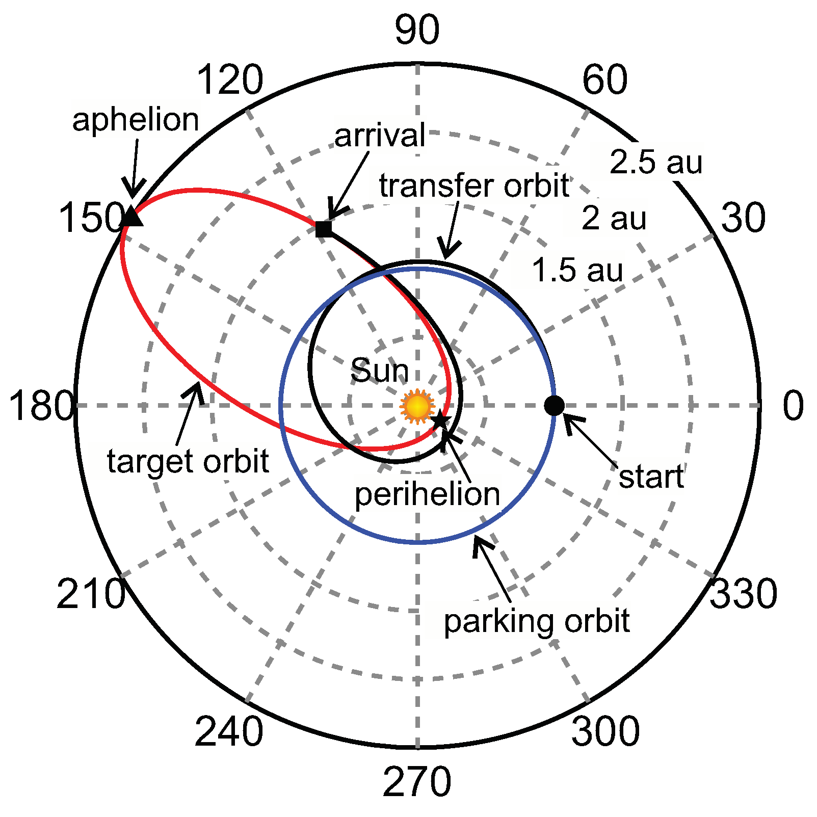
The first strategy is to minimize the transfer time necessary for the spacecraft to reach the heliocentric desired orbit (that is, the elliptic orbit with and ). In this case, the arrival point along the desired orbit is left free and is an output of the optimization process. The time required to complete this phase is , where is the time interval to coast from the insertion point, where the spacecraft enters into the desired orbit, to the orbit perihelion.
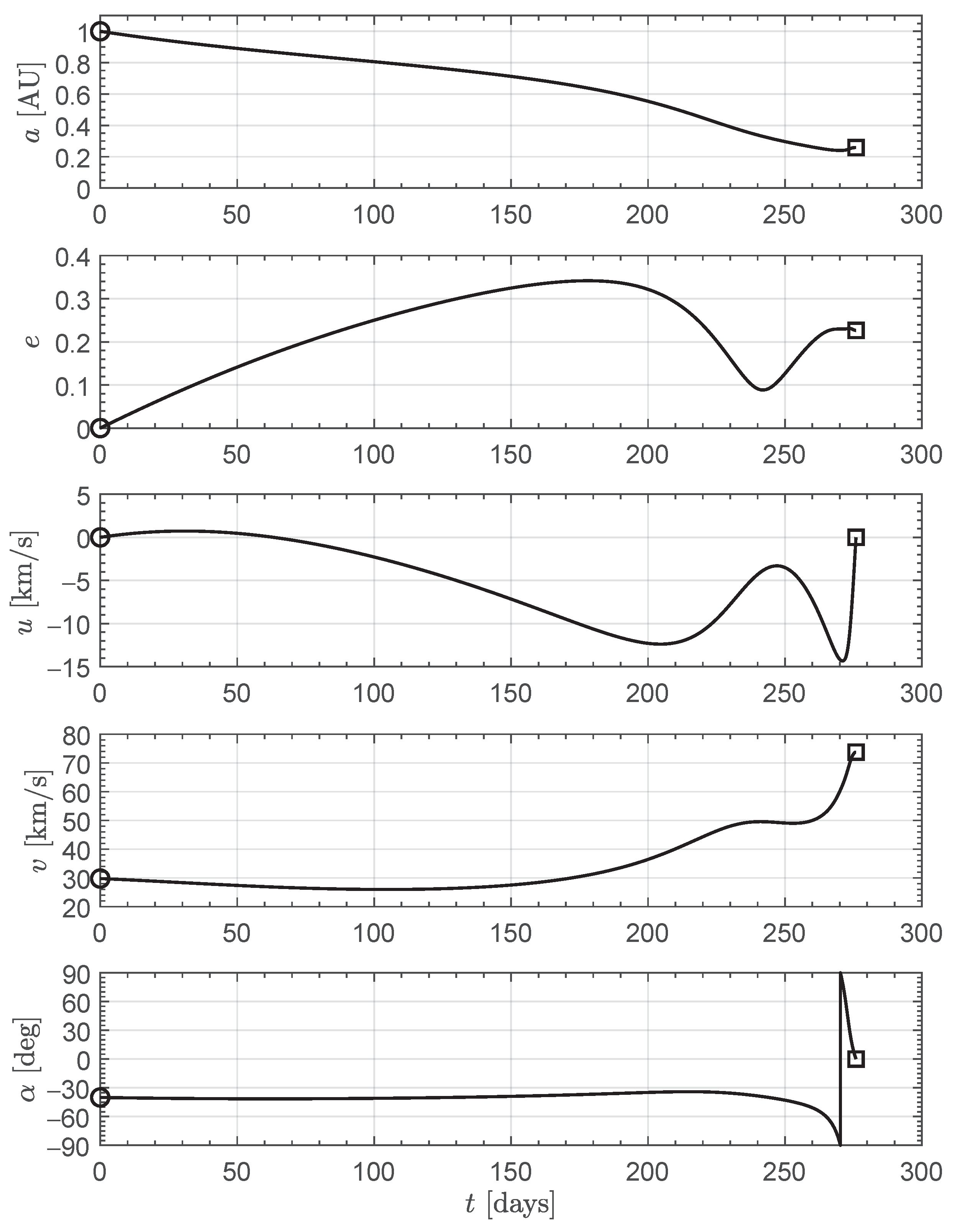
Figure 6 shows the transfer trajectory, where the black square coincides with the arrival, that is, the insertion point along the desired heliocentric orbit. The spacecraft true anomaly at insertion point is roughly . The minimum time to reach the desired orbit is about and the characteristics of the spacecraft osculating orbit during the transfer trajectory are illustrated in Figure 7 along with the optimal sail steering law .
Since the insertion point along the desired orbit is placed forward the perihelion, the spacecraft needs a long time, that is, about , to reach the perihelion with a coasting flight. The total time necessary to complete this phase is roughly .
3.1.2. Case b
The second strategy is to look for the transfer trajectory to the desired orbit with the constraint that the arrival point coincides just with the (desired) orbit perihelion. In this case, the minimum time to reach the perihelion is , which is, of course, greater than of the previous case. Note, however, that because the final point coincides by assumption with the perihelion and no additional coasting phase is required. Figure 8 shows the transfer trajectory, while the characteristics of the spacecraft osculating orbit along the transfer trajectory and the optimal sail steering law are illustrated in Figure 9.
3.1.3. Case c
The third strategy is to minimize the flight time to reach a minimum distance from the Sun of with zero radial velocity, while the transverse velocity is left free. In this case, the minimum transfer time is , with a remarkable time saving (about ) with respect to . However, the final osculating orbit (in red color in Figure 10) has an eccentricity equal to only. Therefore, the transverse velocity at the arrival point, equal to , is substantially smaller than that of cases a and b, where the perihelion velocity is about . Since a high transversal velocity is a fundamental requirement for minimizing the flight time in the succeeding phases, this case actually does not offer an useful option for the whole mission viewpoint. For the sake of completeness Figure 11 shows the characteristics of the spacecraft osculating orbit along the transfer trajectory, the radial and circumferential velocity components and the optimal sail steering law. Note, in particular, that the velocity at the end of the phase is purely circumferential, since the radial component is zero.
3.2. Phase 2
This phase starts when the spacecraft is at a distance equal to from the Sun and, according to the previous analysis, we consider the case 1b, with a starting velocity equal to (fully along the transverse direction). For comparative purposes with the baseline mission, this phase has been studied by minimizing the time required to reach a distance of with the same hyperbolic excess velocity as that reported in [18], that is, . The osculating parameters and the spacecraft velocity components are shown in Figure 12 along with the sail optimal steering law. The flight time in this phase is . Note that the final absolute velocity is nearly radial, that is, the transverse component is , while the radial component is about . The total flight time to reach a distance of from the Sun is therefore .
3.3. Single Optimization of Phases 1 and 2
The previous two phases may be also analyzed within a single optimization problem, by looking for the minimum time trajectory that transfers the spacecraft from the Earth’s (circular) orbit to a heliocentric distance of , where the vehicle arrives with a hyperbolic excess velocity . In this case, the spacecraft initially tends to approach the Sun to exploit a solar photonic assist maneuver that dramatically increases its available thrust [34,35,36,37]. It is therefore necessary to add a constraint on the minimum distance at which the spacecraft pass by the Sun. Details about the practical implementation of such constraint within an optimization problem may be found in [38]. For compatibility purposes with the previous analysis, such a minimum distance is set to , which is equal to the perigee distance of the heliocentric target orbit described in phase 1.
Figure 13 shows that the resulting trajectory is actually tangent to a circle with radius equal to (the forbidden region). The spacecraft reaches the minimum distance from the Sun after about when the transverse velocity takes its maximum value and then quickly decreases, as is shown in Figure 14. Note that in the post-perihelion trajectory the sail is nearly normal to the Sun-spacecraft direction (that is, ) and the spacecraft velocity is almost radial. The total flight time to complete the whole phase is , which is smaller than the sum of the times necessary to complete phases 1 and 2 alone (the time saving is about ). Note that such time saving may be used to increase the hyperbolic excess velocity when the spacecraft reaches the distance of . For example, by solving an optimization problem that maximizes for a fixed flight time, it is possible to look for solutions that provide important improvements over the whole mission time. This parametric analysis will be discussed later on.
3.4. Phase 3
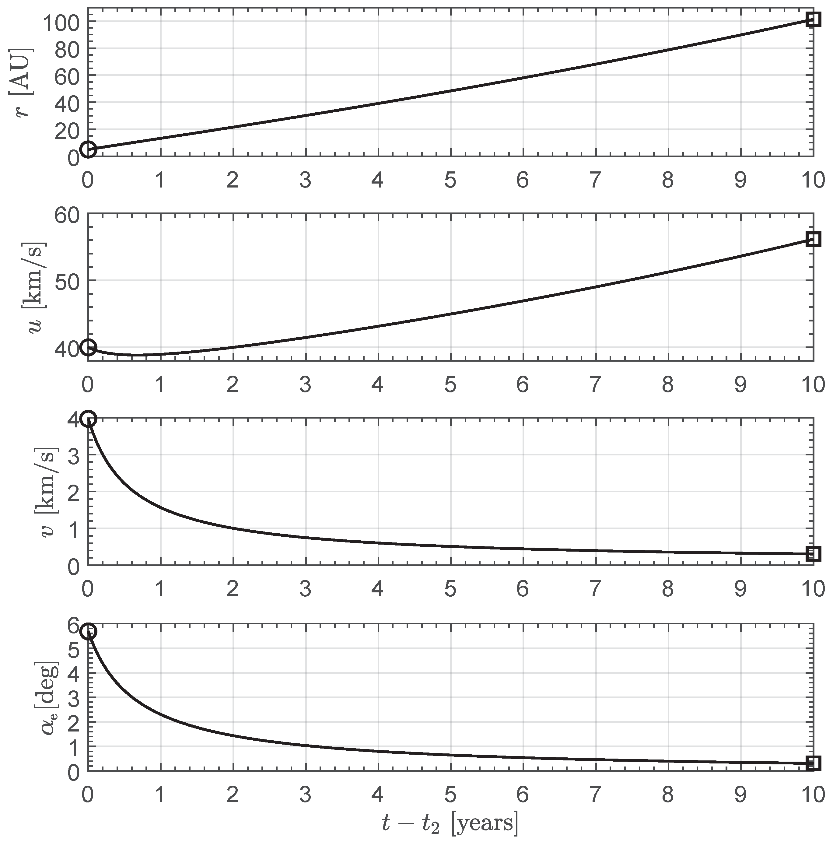
At the end of phase 2 the solar sail becomes ineffective and is therefore jettisoned. The spacecraft is accelerated by the radioisotope-electric thruster that continuously operates for a time length of until the whole xenon propellant is exhausted at a constant mass flow rate. In this part of the mission, the optimization consists in maximizing the hyperbolic excess speed at the phase end. Figure 15 shows the main characteristics of the spacecraft trajectory along with the optimal steering law. The spacecraft eventually reaches a solar distance of with a final hyperbolic excess velocity , equal to that of the baseline mission [18].
3.5. Phase 4
The last trajectory part is a coasting phase with constant velocity in which the spacecraft continues its flight until it reaches a distance of from the Sun. The spacecraft mass in this phase remains constant and equal to . Since the initial hyperbolic excess velocity is the same as that reported in the baseline mission, the time interval necessary to complete this phase is also the same.
The total mission time, that is, the sum of the times necessary to complete the four phases, is equal to . This time interval should be compared with that estimated in the baseline mission, that is . Note that the difference between the optimal time and the flight time in the baseline mission is only due to the time saving obtained in phases 1 and 2. This is a consequence of the assumption according to which the hyperbolic excess velocity at the end of phase 2 is the same as that of the baseline mission. However, the total mission time may be substantially reduced by increasing the value of the hyperbolic excess velocity, as will be shown in the parametric analysis of the next section.
4. Parametric Analysis
Since the longer part of the travel involves the electric-based propulsion phase and the final coasting phase, it is reasonable to look for a different strategy aimed at reducing the flight times in these two mission stages. This is possible by maximizing , that is, the hyperbolic excess velocity at the end of phase 2. The results are shown in Figure 16, where each point in the graph is the solution of an optimal problem in which the final time is fixed.
Note that the results start from (when ), which corresponds to the optimization point of phases 1 and 2. It is clear from the figure that the hyperbolic excess speed may be substantially increased by extending the time interval that exploits the solar photonic assist maneuver. Figure 17 shows how the hyperbolic excess velocity at the end of phase 3 linearly increases with . The effect of a change in the hyperbolic speed is better appreciated in Figure 18, which reports the total mission time as a function of .
The minimum value of the hyperbolic excess velocity in the figure coincides with the one chosen in the baseline mission. When is increased up to the total mission time is , that is, about smaller than that estimated with the baseline mission. Further performance improvements (that is, additional decrease of total mission times) are of course possible by additionally increasing with a prolonged action of the solar sail within phase two. The corresponding trajectories are characterized by multiple revolutions around the Sun to gain as much energy as possible before reaching the required distance of .
5. Conclusions
In this paper, we have analyzed the times necessary to reach the Sun’s gravitational focus with a baseline reference mission taken from Hesperides proposal. To that end, the problem has been studied in an optimal framework, by dividing the mission into a phase in which the spacecraft is propelled by a solar sail, one in which the spacecraft is propelled by an electric thruster, and a final Keplerian arc. The optimal use of a high-performance solar sail in the first phase of the trajectory allows the spacecraft to obtain a hyperbolic excess velocity of in about . The spacecraft is then further accelerated by means of a radioisotope-electric thruster that continuously operates for a time length of and the required distance of is reached in about .
Further performance improvements (in terms of total flight time) are of course possible by additionally increasing the hyperbolic excess velocity using a prolonged phase of solar photonic assist maneuver. The flight times estimated in this study suggest that the Sun’s gravitational focus may be reached in a time interval well below with a near future technology. The natural extension of this paper is to analyze the performance of such a hybrid propulsion system in a more classical (robotic) mission scenario, in which a deep space probe reaches the outer region of the Solar System and the heliopause.
Author Contributions
Conceptualization, G.M. and A.A.Q.; methodology, G.M. and A.A.Q.; software, A.A.Q.; writing—original draft preparation, G.M.; writing—review and editing, G.M. and A.A.Q. All authors have read and agreed to the published version of the manuscript.
Funding
This research received no external funding.
Institutional Review Board Statement
Not applicable.
Informed Consent Statement
Not applicable.
Data Availability Statement
Not applicable.
Conflicts of Interest
The authors declare no conflict of interest.
References
- Matloff, G.L. Von Neumann probes: Rationale, propulsion, interstellar transfer timing. Int. J. Astrobiol. 2022, 1–7. [Google Scholar] [CrossRef]
- Uchaikin, V.V.; Kozhemyakin, I.I. A Mesofractal Model of Interstellar Cloudiness. Universe 2022, 8, 249. [Google Scholar] [CrossRef]
- Kezerashvili, R.Y.; Matloff, G.L.; Long, K.F. Anomalous stellar acceleration: Causes and consequences. JBIS J. Br. Interplanet. Soc. 2021, 74, 269–275. [Google Scholar]
- Miteva, R.; Samwel, S.W.; Zabunov, S. Solar Radio Bursts Associated with In Situ Detected Energetic Electrons in Solar Cycles 23 and 24. Universe 2022, 8, 275. [Google Scholar] [CrossRef]
- Huo, M.; Mengali, G.; Quarta, A.A. Mission Design for an Interstellar Probe with E-Sail Propulsion System. JBIS J. Br. Interplanet. Soc. 2015, 68, 128–134. [Google Scholar]
- Mengali, G.; Quarta, A.A.; Janhunen, P. Considerations of electric sailcraft trajectory design. JBIS J. Br. Interplanet. Soc. 2008, 61, 326–329. [Google Scholar]
- Turyshev, S.; Shao, M.; Alkalai, L.; Freidman, L.; Arora, N.; Weinstein-Weiss, S.; Toth, V. Direct multipixel imaging of an exo-earth with a solar gravitational lens telescope. JBIS J. Br. Interplanet. Soc. 2018, 71, 361–368. [Google Scholar]
- Eshleman, V.R. Gravitational lens of the sun: Its potential for observations and communications over interstellar distances. Science 1979, 205, 1133–1135. [Google Scholar] [CrossRef]
- Heidmann, J.; Maccone, C. ASTROSAIL and SETISAIL: Two extrasolar system missions to the Sun’s gravitational focuses. Acta Astronaut. 1994, 32, 409–410. [Google Scholar] [CrossRef]
- Genta, G.; Vulpetti, G. Some considerations on Sun gravitational lens missions. JBIS J. Br. Interplanet. Soc. 2002, 55, 131–136. [Google Scholar]
- Maccone, C. Realistic targets at 1000 AU for interstellar precursor missions. Acta Astronaut. 2010, 67, 526–538. [Google Scholar] [CrossRef]
- Maccone, C. Deep Space Flight and Communications Exploiting the Sun as a Gravitational Lens; Springer Praxis Books; Springer: Berlin/Heidelberg, Germany, 2009. [Google Scholar] [CrossRef] [Green Version]
- Friedman, L.; Turyshev, S. First stop on the interstellar journey: The solar Gravity Lens Focus. JBIS J. Br. Interplanet. Soc. 2018, 71, 275–279. [Google Scholar]
- Matloff, G.L. The Solar-Electric Sail: Application to Interstellar Migration and Consequences for SETI. Universe 2022, 8, 252. [Google Scholar] [CrossRef]
- Landis, G.A. Mission to the Gravitational Focus of the Sun: A Critical Analysis. In Proceedings of the AIAA SciTech Forum—55th AIAA Aerospace Sciences Meeting, Grapevine, TX, USA, 9–13 January 2017. [Google Scholar] [CrossRef] [Green Version]
- Murzionak, P.; Welch, C.; Matloff, G.L. The oculus project: Gravitational lensing, earth-like exoplanets and solar sailing. JBIS J. Br. Interplanet. Soc. 2016, 69, 439–449. [Google Scholar]
- Turyshev, S.G.; Shao, M.; Toth, V.T.; Friedman, L.D.; Alkalai, L.; Mawet, D.; Shen, J.; Swain, M.R.; Zhou, H.; Helvajian, H.; et al. Direct Multipixel Imaging and Spectroscopy of an Exoplanet with a Solar Gravity Lens Mission. arXiv 2020, arXiv:2002.11871. [Google Scholar]
- Matloff, G.L. Hesperides: Solar/nuclear missions to the Sun’s inner gravity focus. Acta Astronaut. 2014, 104, 477–479. [Google Scholar] [CrossRef]
- Matloff, G.L.; Johnson, L.; Maccone, C. Helios and prometheus: A solar/nuclear outer-solar system mission. JBIS J. Br. Interplanet. Soc. 2007, 60, 439–442. [Google Scholar]
- Quarta, A.A.; Mengali, G. Analytical Results for Solar Sail Optimal Missions with Modulated Radial Thrust. Celest. Mech. Dyn. Astron. 2011, 109, 147–166. [Google Scholar] [CrossRef]
- Bassetto, M.; Caruso, A.; Quarta, A.A.; Mengali, G. Optimal heliocentric transfers of a Sun-facing heliogyro. Aerosp. Sci. Technol. 2021, 119, 107094. [Google Scholar] [CrossRef]
- Bassetto, M.; Quarta, A.A.; Mengali, G.; Cipolla, V. Trajectory Analysis of a Sun-Facing Solar Sail with Optical Degradation. J. Guid. Control. Dyn. 2020, 43, 1727–1732. [Google Scholar] [CrossRef]
- Bassetto, M.; Niccolai, L.; Boni, L.; Mengali, G.; Quarta, A.A.; Circi, C.; Pizzurro, S.; Pizzarelli, M.; Pellegrini, R.C.; Cavallini, E. Sliding Mode Control for Attitude Maneuvers of Helianthus Solar Sail. Acta Astronaut. 2022, 198, 100–110. [Google Scholar] [CrossRef]
- Wright, J.L. Space Sailing; Gordon and Breach Science Publishers: London, UK, 1992; pp. 223–233. ISBN 978-2881248429. [Google Scholar]
- McInnes, C.R. Solar Sailing: Technology, Dynamics and Mission Applications; Springer-Praxis Series in Space Science and Technology; Springer: Berlin, Germany, 1999; Chapter 2; pp. 46–54. [Google Scholar] [CrossRef]
- Dachwald, B.; Macdonald, M.; McInnes, C.R.; Mengali, G.; Quarta, A.A. Impact of optical degradation on solar sail mission performance. J. Spacecr. Rocket. 2007, 44, 740–749. [Google Scholar] [CrossRef]
- Dachwald, B.; Mengali, G.; Quarta, A.A.; Macdonald, M. Parametric model and optimal control of solar sails with optical degradation. J. Guid. Control. Dyn. 2006, 29, 1170–1178. [Google Scholar] [CrossRef]
- Niccolai, L.; Quarta, A.A.; Mengali, G. Trajectory Approximation of a Solar Sail with Constant Pitch Angle and Optical Degradation. IEEE Trans. Aerosp. Electron. Syst. 2022; in press. [Google Scholar] [CrossRef]
- Bianchi, C.; Niccolai, L.; Mengali, L.; Quarta, A.A. Collinear artificial equilibrium point maintenance with a wrinkled solar sail. Aerosp. Sci. Technol. 2021, 119, 107150. [Google Scholar] [CrossRef]
- Mengali, G.; Quarta, A.A.; Circi, C.; Dachwald, B. Refined solar sail force model with mission application. J. Guid. Control. Dyn. 2007, 30, 512–520. [Google Scholar] [CrossRef] [Green Version]
- Mengali, G.; Quarta, A.A. Optimal three-dimensional interplanetary rendezvous using nonideal solar sail. J. Guid. Control. Dyn. 2005, 28, 173–177. [Google Scholar] [CrossRef]
- Mengali, G.; Quarta, A.A. Solar Sail Trajectories with Piecewise-Constant Steering Laws. Aerosp. Sci. Technol. 2009, 13, 431–441. [Google Scholar] [CrossRef]
- Quarta, A.A.; Mengali, G. Minimum-Time Space Missions with Solar Electric Propulsion. Aerosp. Sci. Technol. 2011, 15, 381–392. [Google Scholar] [CrossRef]
- Leipold, M.; Wagner, O. ‘Solar Photonic Assist’ Trajectory Design for Solar Sail Missions to the Outer Solar System and Beyond. In Proceedings of the Spaceflight Dynamics 1998, Advances in Astronautical Sciences, Greenbelt, MD, USA, 11–15 May 1998; Stengle, T.H., Ed.; AAS/GSFC International Symposium on Space Flight Dynamics, Univelt: Greenbelt, MD, USA, 1998; Volume 100, Part 1. pp. 1035–1046. [Google Scholar]
- Lyngvi, A.; Falkner, P.; Kemble, S.; Leipold, M.; Peacock, A. The Interstellar Heliopause Probe. Acta Astronaut. 2005, 57, 104–111. [Google Scholar] [CrossRef]
- Sauer, C.G., Jr. Solar Sail Trajectories for Solar Polar and Interstellar Probe Missions. In Proceedings of the AAS/AIAA Astrodynamics Specialist Conference, Girdwood, AK, USA, 15–19 August 1999. [Google Scholar]
- Wallace, R.A.; Ayon, J.A.; Sprague, G.A. Interstellar Probe Mission/System Concept. In Proceedings of the 2000 IEEE Aerospace Conference, Big Sky, MT, USA, 25 March 2000; Volume 7, pp. 385–396. [Google Scholar] [CrossRef]
- Quarta, A.A.; Mengali, G. Electric Sail Mission Analysis for Outer Solar System Exploration. J. Guid. Control. Dyn. 2010, 33, 740–755. [Google Scholar] [CrossRef]
Figure 1.
Sun’s gravitational lens position. Background image courtesy of Johns Hopkins APL.

Figure 2.
Clusters of small satellites in a string-of-pearls arrangement towards the Sun’s gravitational lens. Courtesy of and reprinted with permission of The Aerospace Corporation.
Figure 2.
Clusters of small satellites in a string-of-pearls arrangement towards the Sun’s gravitational lens. Courtesy of and reprinted with permission of The Aerospace Corporation.

Figure 3.
Mass breakdown model for Hesperides spacecraft [18].
Figure 3.
Mass breakdown model for Hesperides spacecraft [18].

Figure 4.
Graphical sketch and spacecraft mass variation of Hesperides baseline mission [18].
Figure 4.
Graphical sketch and spacecraft mass variation of Hesperides baseline mission [18].

Figure 5.
Reference frame and unit vectors.

Figure 6.
Minimum-time transfer trajectory to reach the heliocentric desired orbit (case a).

Figure 7.
Osculating parameters of the transfer orbit and optimal (sail) steering law (case a).

Figure 8.
Minimum-time transfer trajectory to the perigee of the desired orbit (case b).

Figure 9.
Osculating parameters of the transfer orbit and optimal steering law (case b).

Figure 10.
Minimum-time transfer trajectory to reach a heliocentric distance of with zero radial velocity (case c).
Figure 10.
Minimum-time transfer trajectory to reach a heliocentric distance of with zero radial velocity (case c).

Figure 11.
Osculating parameters of the transfer orbit, spacecraft velocity components and optimal steering law to reach a distance of with zero radial velocity (case c).
Figure 11.
Osculating parameters of the transfer orbit, spacecraft velocity components and optimal steering law to reach a distance of with zero radial velocity (case c).

Figure 12.
Osculating parameters of the transfer orbit, spacecraft velocity components and optimal steering law to reach a distance of with .
Figure 12.
Osculating parameters of the transfer orbit, spacecraft velocity components and optimal steering law to reach a distance of with .

Figure 13.
Minimum-time transfer trajectory to reach a heliocentric distance of with a hyperbolic excess velocity .
Figure 13.
Minimum-time transfer trajectory to reach a heliocentric distance of with a hyperbolic excess velocity .

Figure 14.
Heliocentric distance, velocity components and optimal steering law to reach a distance of with .
Figure 14.
Heliocentric distance, velocity components and optimal steering law to reach a distance of with .

Figure 15.
Heliocentric distance, velocity components and optimal steering law in phase 3.

Figure 16.
Flight time necessary to complete phases 1 and 2 as a function of the hyperbolic excess velocity at the end of phase 2.
Figure 16.
Flight time necessary to complete phases 1 and 2 as a function of the hyperbolic excess velocity at the end of phase 2.

Figure 17.
Hyperbolic excess velocity at the end of phase 3 as a function of that at the end of phase 2.
Figure 17.
Hyperbolic excess velocity at the end of phase 3 as a function of that at the end of phase 2.

Figure 18.
Total mission time as a function of the hyperbolic excess velocity at the end of phase 2.
Figure 18.
Total mission time as a function of the hyperbolic excess velocity at the end of phase 2.


Table 1.
Hesperides spacecraft subsystems mass [18].
Table 1.
Hesperides spacecraft subsystems mass [18].
| Subsystem | Mass (kg) |
|---|---|
| Solar sail | 201 |
| Ion thruster | 10 |
| Radioisotope electric generator | 40 |
| Propellant | 100 |
| Payload | 99 |
| Total | 450 |
Publisher’s Note: MDPI stays neutral with regard to jurisdictional claims in published maps and institutional affiliations. |
© 2022 by the authors. Licensee MDPI, Basel, Switzerland. This article is an open access article distributed under the terms and conditions of the Creative Commons Attribution (CC BY) license (https://creativecommons.org/licenses/by/4.0/).
Share and Cite
MDPI and ACS Style
Mengali, G.; Quarta, A.A. Trajectory Analysis and Optimization of Hesperides Mission. Universe 2022, 8, 364. https://doi.org/10.3390/universe8070364
AMA Style
Mengali G, Quarta AA. Trajectory Analysis and Optimization of Hesperides Mission. Universe. 2022; 8(7):364. https://doi.org/10.3390/universe8070364
Chicago/Turabian StyleMengali, Giovanni, and Alessandro A. Quarta. 2022. "Trajectory Analysis and Optimization of Hesperides Mission" Universe 8, no. 7: 364. https://doi.org/10.3390/universe8070364
Note that from the first issue of 2016, this journal uses article numbers instead of page numbers. See further details here.