
Geodesic Structure of Generalized Vaidya Spacetime through the K-Essence

1
Department of Mathematics, Prabhat Kumar College, Contai 721404, India
2
Institute of Physics, Southern Federal University, 194 Stachki, Rostov-on-Don 344090, Russia
3
Department of Physics, National Research Nuclear University, MEPHI, Moscow 115409, Russia
4
Virtual Institute of Astroparticle Physics, Rue Garreau, 75018 Paris, France
5
Centre for Cosmology, Astrophysics and Space Science (CCASS), GLA University, Mathura 281406, India
6
Department of Physics, Prabhat Kumar College, Contai 721404, India
7
Institute of Astronomy, Space and Earth Science (IASES), Kolkata 700054, India
*
Author to whom correspondence should be addressed.
Universe 2023, 9(12), 510; https://doi.org/10.3390/universe9120510
Submission received: 6 November 2023
/
Revised: 5 December 2023
/
Accepted: 6 December 2023
/
Published: 8 December 2023
(This article belongs to the Special Issue Universe: Feature Papers 2023—Cosmology)
Abstract
:This article investigates the radial and non-radial geodesic structures of the generalized K-essence Vaidya spacetime. Within the framework of K-essence geometry, it is important to note that the metric does not possess conformal equivalence to the conventional gravitational metric. This study employs a non-canonical action of the Dirac–Born–Infeld kind. In this work, we categorize the generalized K-essence Vaidya mass function into two distinct forms. Both the forms of the mass functions have been extensively utilized to analyze the radial and non-radial time-like or null geodesics in great detail inside the comoving plane. Indications of the existence of wormholes can be noted during the extreme phases of spacetime, particularly in relation to black holes and white holes, which resemble the Einstein–Rosen bridge. In addition, we have also detected a distinctive indication of the quantum tunneling phenomenon around the singularity (). Furthermore, we have found that for certain types of solutions, there exist circular orbits through the event horizon as well as quasicircular orbits. Also, we have noted that there is no central singularity in our spacetime where both r and t tend towards zero. The existence of a central singularity is essential for any generalized Vaidya spacetime. This indicates that spacetime can be geodesically complete, which correlates with the findings of Kerr’s recent work (2023).
1. Introduction
Chandrasekhar extensively analyzed the time-like and null geodesic features of the Schwarzschild spacetime in his book [1]. In addition, he examined the orbital configurations of both the confined and unconfined trajectories using graphical representations. In addition, the authors of [2] examined the geodesic structures of the Schwarzschild anti-de Sitter spacetime. The researchers assessed both radial and non-radial paths for time-like and null geodesics. Additionally, they demonstrated that the geodesic structures of this black hole exhibit distinct forms of motion that are not permitted by the Schwarzschild spacetime. The geometric framework of the Schwarzschild spacetime is also examined in [3]. The Jacobi metric for time-like geodesics in static spacetimes was examined in Ref. [4]. They demonstrated that the unrestricted movement of large particles in stationary spacetimes is determined by the geodesics of a Riemannian metric that depends on the particle’s energy. This metric is similar to Jacobi’s metric in classical dynamics. When the mass of an object approaches zero, Jacobi’s metric becomes identical to the Fermat or optical metric, which does not depend on energy. In addition, they provided a detailed account of the characteristics of the Jacobi metric pertaining to the motion of heavy particles beyond the event horizon of a Schwarzschild black hole. The authors of [5] derived the Jacobi metric for different stationary metrics and developed the Jacobi–Maupertuis metric for time-dependent metrics by using the Eisenhart–Duval lift [6,7]. The authors of [8] documented the remarkable characteristics of the time-like geodesic structure when dark energy is present in an emergent gravity framework, specifically for the Barriola–Vilenkin metric [9]. The K-essence emergent gravity metric is precisely correlated with the Barriola–Vilenkin (BV) metric for the Schwarzschild background, specifically for a certain form of K-essence scalar field [10]. The researchers analyzed the various paths that time-like geodesics can take in the presence of dark energy in the Barriola–Vilenkin spacetime [8], which is equivalent to the Schwarzschild spacetime in terms of its fundamental structure. However, the permissible ranges for the maximum and minimum distances from the central object are significantly distinct. For a constant dark energy density, the orbits, both bound and unbound, were graphed.
In 1951, Vaidya proposed the first relativistic line element that properly represented the spacetime of a conceivable star [11]. It extended the specific solution of Schwarzschild by depicting the emission of radiation for a mass that is not in a static state. The Schwarzschild solution describes the geometry of spacetime around a spherically symmetric, non-rotating, black object with a constant mass. Therefore, it is clear that the model is incapable of accurately depicting spacetime outside the confines of a star. The solution proposed by Vaidya [11], known as the Vaidya spacetime or the radiating Schwarzschild metric, was introduced as a possible explanatory framework. The main distinction between the two metrics is that the Vaidya metric adds a time-dependent mass parameter, whereas the Schwarzschild metric uses a constant mass value. As a result, the spacetime in the Vaidya metric evolves with time. The Vaidya metric is primarily used to investigate gravitational collapse. The occurrence of gravitational collapse is widely acknowledged in the disciplines of general relativity and astrophysics, as demonstrated by the research conducted by Joshi et al. [12,13,14,15,16,17,18,19]. It plays a vital role in understanding several astrophysical aspects of our cosmos. The phenomenon of gravitational collapse provides useful insights into several elements of astronomy, including the evolution of structures, the features of stars, the genesis of black holes, and the construction of white dwarfs or neutron stars, among other events. Gravitational collapse refers to the phenomenon in which a star collapses as a result of its mass. The outcome of this collapse might vary depending on the exact beginning mass conditions, leading to distinct stages of collapse. Papapetrou [20] was the first to demonstrate that the solution of a null dust fluid with spherical symmetry in gravitational collapse can lead to the creation of naked singularities. This statement presents a counterexample of the cosmic censorship hypothesis (CCH) as proposed by Penrose [21,22]. The authors of [14,23] provided a detailed account of the causal paths that connect the singularities in the continuing Vaidya scenario. Furthermore, a comprehensive classification of the non-space-like geodesics that link the naked singularity in the past is presented, offering a rather thorough discussion of the restrictions involved. It is subsequently demonstrated to be a robust curvature singularity in a more significant manner.
The Vaidya solution, as a generalization, encompasses all the established solutions of Einstein’s field equations that include a mix of type-I and type-II matter fields [24,25,26,27,28,29]. The composition of this work is attributed to Husain [30] and Wang and Wu [31]. The extension of the Vaidya solution is sometimes referred to as the generalized Vaidya spacetime. The work performed in [32] examines the gravitational collapse of the generalized Vaidya spacetime within the framework of the cosmic censorship theory. They demonstrated that the categories of generalized Vaidya mass functions emerged in the situation, suggesting the end of collapse with a locally visible central singularity. The authors computed the magnitude of these singularities. A comprehensive mathematical framework was created to examine the requirements for the mass function for non-space-like geodesics going towards the future to end at the singularity in the past. Furthermore, they demonstrated that, when considering a certain generalized Vaidya mass function, the ultimate outcome of the collapse can be precisely defined as either a black hole or a naked singularity. The work by Patil [33] examined the phenomenon of gravitational collapse in higher dimensions within the context of the charged Vaidya spacetime. It was demonstrated that singularities occur in a charged null fluid in a higher dimension. These singularities consistently lacked any form of covering, hence contradicting the strong CCH. This idea does not specifically pertain to weak cosmic censorship. The Vaidya metric has received significant attention in scholarly research, with several major contributions to our comprehension of this subject. The authors of the study [34] examined the geometric properties of Vaidya’s spacetime while considering a white hole that undergoes a decrease in mass. They found that the white hole can either stabilize and transform into a black hole within a limited or indefinite amount of time, or entirely evaporate. The researchers focused specifically on the scenario of total evaporation over an indefinite period of time. They successfully demonstrated the presence of an asymptotic light-like singularity in the conformal curvature, which connects both the past space-like singularity and the future time-like infinity. Vertogradov [35] conducted a study on the structure of the generalized Vaidya spacetime, specifically focusing on the case when the matter field of type-II follows the equation of state . The findings of the study revealed the presence of an eternal naked singularity in this spacetime, which meets all energy conditions. Once formed, the singularity will remain perpetually uncovered by the apparent horizon. Nevertheless, the formation of the apparent horizon leads to the emergence of a white hole. Solanki et al. [36] derived precise mathematical equations that describe the changes in the photon sphere and the angular radius of the shadow in a certain Vaidya spacetime. The mass function was seen as a function of time that either increases or decreases linearly. The initial scenario can function as a basic representation of a black hole that is accumulating matter, whereas the subsequent scenario can be seen as an illustration of a black hole that is emitting radiation, as theorized by Hawking.
In the realm of K-essence geometry, Manna et al. [37] were the first to establish a link between K-essence geometry and Vaidya spacetime. They achieved this by introducing a new definition of the generalized Vaidya mass function, which directly depends on the kinetic energy of the K-essence scalar field. Subsequently, Manna et al. [38] demonstrated that the K-essence emergent gravity metric bears a strong resemblance to the recently found generalized Vaidya metrics for the collapse of a null fluid. This similarity arises from the presence of a K-essence emergent mass function. Notably, Manna’s analysis exclusively considers the K-essence scalar field as a function of either the advanced or the retarded time. The recently developed K-essence model, known as the K-essence emergent Vaidya spacetime, has successfully met all the necessary energy conditions. The presence of the centrally exposed singularity and the intensity and stability of the singularities in the K-essence emergent Vaidya metric yield intriguing results in their research. The evaporation of the dynamical horizon with the Hawking temperature in the K-essence Vaidya Schwarzschild spacetime was investigated by Manna et al. in [39]. This study uses the dynamical horizon equation to quantify the reduction in mass caused by Hawking radiation. Additionally, the tunneling formalism, namely, the Hamilton–Jacobi technique, is utilized to compute the Hawking temperature. In addition, Sawayama’s revised explanation of the dynamical horizon [40] is utilized to demonstrate that the results obtained differ from the conventional Vaidya spacetime geometry. The authors establish, using analytical measures, that the mass of the black hole, denoted as , in the K-essence emergent Schwarzschild–Vaidya spacetime, consistently decreases over time but does not fully evaporate.
The K-essence theory is a scalar field model that deviates from the canonical form. In this theory, the dominant energy component of the field is its kinetic energy, rather than its potential energy. This concept and related others have been extensively studied by several researchers [41,42,43,44,45,46,47,48,49,50,51,52]. The distinctions between the K-essence theory employing a non-canonical Lagrangian and the relativistic field theories utilizing a canonical Lagrangian are found in the sophisticated dynamical solutions of the K-essence equation of motion. These solutions not only spontaneously violate Lorentz invariance but also alter the metric for the perturbations around them. The disturbances propagate in the emergent or analogous curved spacetime, characterized by a metric distinct from the gravitational metric. The non-canonical Lagrangian may be expressed as , where , is the K-essence scalar field, and is the potential term. An alternate form of the Lagrangian, as described by Tian [53], may be represented as , where , and are constants, , and and are arbitrary functions. The functions and are unrestricted and can have any form. Furthermore, it is important to mention that there exist examples of K-essence theories that are not minimally linked, as mentioned in Refs. [54,55,56]. Nevertheless, this article only addresses the minimally coupled K-essence theory, as investigated in Refs. [41,42,43,44,45,46,47,48,49,50]. In a general sense, the Lagrangian has the capacity to depend on any functions of and X. The K-essence theory offers the benefit of circumventing both the fine-tuning problem and the coincidence problem [57] of the current universe. Additionally, it generates the negative pressure required for the universe’s acceleration only through the kinetic energy of the field. The kinetic term of the field dominates over the potential term. The article [41] presents attractor solutions where the dynamics of the cosmos are governed by the scalar field of the models. During the radiation-dominated phase, the K-essence field mimics the equation of state of radiation and has a constant ratio to the radiation density. The K-essence field is unable to replicate the dust-like equation of state (EOS) due to dynamical limits during the time dominated by dust. However, it rapidly reduces its energy value by many orders of magnitude and eventually reaches a constant value. Subsequently, over a period approximately equivalent to the current age of the universe, the density of matter is diminished by the K-essence field, leading to the commencement of cosmic acceleration. The equation of state (EOS) of the K-essence theory ultimately converges to a value within the range of 0 to −1. Although, in theory, it has the potential to extend beyond . Another intriguing aspect of the K-essence idea is its potential to generate a type of dark energy where the speed of sound is consistently slower than that of light. This feature may mitigate the cosmic microwave background (CMB) disruptions on large angular scales [58,59,60]. In this specific situation, Manna and coworkers [8,10,37,38,39,61,62,63,64,65,66] have developed a fascinating emergent gravity metric, referred to as . This metric possesses distinct attributes in contrast to the standard gravitational metric and is derived from the notions of the Dirac–Born–Infeld (DBI)-type action, as outlined in Refs. [67,68,69,70]. Dirac et al. [70] proposed a non-canonical Lagrangian in order to eliminate the infinite self-energy of the electron, as described in their work. The specific reasons and objectives for selecting the non-canonical theory, such as the K-essence theory, may be found in Refs. [71,72]. The Planck collaborations’ findings, as shown in Refs. [73,74,75], have examined the empirical evidence supporting the concept of K-essence with a DBI-type non-canonical Lagrangian, along with other modified theories. Furthermore, it has been noted that the K-essence theory may be applied in a model that combines dark energy and dark matter [8,10,45,61,62,63,64], as well as from a purely gravitational perspective [37,38,39,65,66].
This article is organized as follows: in Section 2, we provided a concise explanation of the K-essence geometry and its connection to the conventional generalized Vaidya spacetime, which leads to the construction of a new generalized K-essence Vaidya spacetime. Section 3 offers a comprehensive analysis of the geodesic structures observed in the generalized K-essence Vaidya spacetime. This analysis considers two forms of mass function while ensuring that the condition on the kinetic energy of the K-essence scalar field is maintained. This section also provides a detailed analysis of the radial and non-radial geodesics used to examine the structure of time-like and null geodesics in the given spacetime. This is achieved by solving the Euler–Lagrange equations. A graphical and numerical analysis is also performed in this section. In Section 4, we wrap up both the discussion and conclusions.
2. Summary of the Relation between K-Essence and Generalized Vaidya Spacetime
This section offers a short introduction to the geometry of K-essence and the generalized Vaidya spacetime. Initially, we present a brief summary of the geometric aspects related to the K-essence, as extensively explored in many scholarly references [41,42,43,44,45,46,47,48,49,50]. The action performed by the minimally couple K-essence geometry is
where the expression represents the canonical kinetic term, whereas denotes the non-canonical Lagrangian. In this scenario, the conventional gravitational metric has formed a minimum coupling with the K-essence scalar field ().
The energy–momentum tensor that corresponds solely to the K-essence scalar field is
where and is the covariant derivative defined with respect to the gravitational metric .
The equation of motion (EOM) for the K-essence scalar field is
where
with and .
Equations (4) and (5) have physical relevance when is non-zero, assuming a positive definite . Equation (5) states that the emergent metric, represented as , differs in its conformal properties from the metric when considering non-trivial configurations of the scalar field . Like canonical scalar fields, the variable exhibits diverse local causal structural properties. It also differs from those that are defined using . The EOM, as stated in Equation (3), is valid even when taking into account the implicit relationship between L and . Then, the EOM Equation (3) is
This study addresses the Dirac–Born–Infeld (DBI)-type non-canonical Lagrangian, which is represented as [8,10,37,67,68,69,70,71,72]
The K-essence paradigm posits that the prevalence of kinetic energy over potential energy results in the exclusion of the potential term in the Lagrangian Equation (7) [67,71,72]. The squared speed of sound, represented as , is determined by the expression . Therefore, Equation (5) for the effective emergent metric is expressed as
since is a scalar.
The Christoffel symbol, corresponding to the emergent gravity metric given by Equation (8), can be written as [8,10,71,72]
where is the usual Christoffel symbol associated with the gravitational metric .
Hence, the geodesic equation governing the K-essence geometry may be expressed as
where is an affine parameter.
The covariant derivative [48,71,72] linked with the emergent metric gives
and the inverse emergent metric is , such as .
Therefore, considering the extensive behavior that defines the dynamics of K-essence and general relativity [47,71,72], the emergent Einstein equation (EEE) may be formulated as
where is constant, is the Ricci tensor, and is the Ricci scalar. Moreover, the energy–momentum tensor is linked to this emergent spacetime.
Now, we would like to provide a concise overview of the K-essence emergent generalized Vaidya spacetime. In the cited work [38], the author introduced the concept of K-essence emergent generalized Vaidya spacetime. This framework considers the background gravitational metric to be the typical generalized Vaidya metric [30,31], while also satisfying the necessary energy requirements. The line element for the emergent generalized Vaidya metric in K-essence theory is as follows:
with .
They defined the K-essence emergent Vaidya mass function:
where is the usual generalized Vaidya mass function and () is the non-zero kinetic energy of the K-essence scalar field.
The above-mentioned mass function pertains to the gravitational energy associated with the K-essence emergent gravity within a specified radius r. Here, we substitute the Eddington advanced time coordinate with the conventional time coordinate, without any loss of generality, denoted as . In this study [38], the author examined the effective K-essence emergent metric, as denoted by Equation (8). Additionally, the author calculated all the components of the EEE (Equation (12)) and the necessary energy conditions. It is important to mention that the assumption about contradicts local Lorentz invariance since, in general, spherical symmetry only requires . The inclusion of the assumption of the independence of , denoted as , suggests that beyond this specific frame selection, a spherically symmetric is indeed a function of both t and r. The K-essence theory permits the occurrence of Lorentz violation due to the fact that the dynamic solutions of the K-essence equation of motion spontaneously break Lorentz invariance and alter the metric for the perturbations around these solutions.
Furthermore, the authors of [37] successfully established a connection between the geometry of K-essence and the Vaidya spacetime. The researchers developed a model of the Vaidya spacetime with generalized K-essence, which takes into account any spherically symmetric static black hole as the underlying spacetime. The line element of the new geometry is (using Equation (8))
gives the mass function
In this article [37], the authors also calculated all the components of the EEE and the required energy conditions. If we consider , i.e., the background physical spacetime is Schwarzschild spacetime, the mass function may be expressed as
Again, if we select the function , Q represents the charge of the Reissner–Nordström (RN) black hole in the physical spacetime. In this case, the related mass function [37] is modified as
It is important to mention that the values of must be between 0 and 1. Otherwise, the metric (13) and (15) cannot be specified properly, and the presence of a dynamical horizon is also questionable [37,38]. In order to maintain the energy conditions, it is evident that the must be a monotonically increasing function of t, with the condition . The admissible configurations for the K-essence scalar field in the generalized Vaidya solution, in order to have a dynamical horizon, are subject to a highly restrictive constraint. It is important to note that the metrics mentioned above represent dynamical horizons rather than isolated or event horizons, as explained extensively in Refs. [37,38].
It is also noted that the time dependence in the given mass functions (Equations (17) and (18)) arises from the kinetic energy of the K-essence scalar field. However, in the mass function Equation (14), the time dependence comes from both the usual generalized Vaidya mass and the K-essence scalar fields. Thus, considering the above situations of the K-essence generalized Vaidya spacetime, we may conclude that the K-essence Vaidya mass function adheres to the general form specified in Equation (14). Therefore, we may conclude that the background metric can be chosen from any standard gravitational metric, with the only alteration being the replacement of their masses with a background mass, which likewise satisfies the EEE equation.
3. Geodesics for the Generalized K-Essence Vaidya Spacetime
This section focuses on analyzing the geodesic structure of the generalized K-essence Vaidya spacetime. In this context, we define our investigative metric as Equation (13), where the K-essence emergent Vaidya mass function is represented by Equation (14). For metric (13), we can write the Lagrangian as [1,8,35,36]
where , is to be identified with the proper time.
Now, using the Euler–Lagrange equation we have
where and we write as .
Because our object and metric are spherically symmetric, we can simplify everything by examining just motion on the equatorial plane and, therefore, . For the above choice of equatorial plane, Equation (22) becomes
Thus, by employing Equation (24) on the equatorial plane, we may write from Equation (19) that the Lagrangian is
Due to the inclusion of the generalized K-essence Vaidya mass function () in the Lagrangian formulation provided above, further analysis is not possible as it can have varying values based on the gravitational mass. Within this particular situation, we have the option to select the mass function. For our subsequent analysis, we have selected two distinct mass functions. Moreover, it is mentioned that the K-essence Vaidya mass function (14) depends on , which has values between 0 and 1. Therefore, we can select as an explicit function of the time in order to keep the values of throughout the article as [37]
where is a positive constant.
3.1. Case-I:
In this subsection, we will look at the K-essence Vaidya mass function as
where M is the mass of a Schwarzschild black hole.
In this scenario, the time dependence of the mass parameter is derived from the K-essence scalar field via Equation (26), which was previously discussed in the preceding section. For this mass function (27), the radii of the dynamical horizon can be written as and (see Appendix A). Given that the mass parameter in Equation (25) is directly influenced by the time through Equations (14) and (26), we may infer from Refs. [35,36] that the energy E can be expressed as a function of the time t:
The solution of the aforementioned equation, as denoted by Equation (29), is highly intricate and cannot be solved directly. To determine the expression for in the above equation, we converted our measurement to a comoving plane, where . This conversion is consistently maintained throughout the article. Thus, on the comoving plane (), the expression for is
Thus, we can say that in our model, specifically when we select a specific form (26) for the kinetic energy of the K-essence scalar field while satisfying the imposed conditions, we have found a direct relationship between the energy of the system we have chosen and the kinetic energy of the K-essence scalar field in the comoving plane. So, the K-essence Vaidya mass function (27) can be written as
It is important to point out that the Vaidya metric defines the gravitational field surrounding a massive object, often a dying star, that emits radiation in the form of null dust. The notion of the Vaidya spacetime is expanded in the generalized version to encompass a wide range of scenarios, accommodating different forms of matter and radiation. The spacetime is dynamic and undergoes evolution as matter compresses, with the metric describing the changing curvature [30,31]. Within the framework of the generalized Vaidya spacetime, employing comoving observers that satisfy the condition “” simplifies the mathematical representation of the spacetime. This enables us to utilize a temporal reference that tracks the movement of matter as it undergoes gravitational collapse to become a black hole or emits radiation as a star. Using a time parameter that evolves with the behavior of matter is a practical approach for investigating gravitational collapse or radiating stars. It improves the intuitiveness and physical significance of describing the collapse process. While examining geodesic structures in the generalized Vaidya spacetime from the perspective of a comoving observer, our focus lies on the trajectories that objects or particles take when they deal with the changing spacetime caused by the reducing matter. These geodesics illustrate the paths that things follow as they move through spacetime, which is influenced by changes in curvature caused by the dynamics of matter. Comprehending these geodesic structures is essential for analyzing the dynamics of particles, photons, and observers in spacetime. It facilitates forecasting the movement and interaction of objects inside the gravitational field generated by collapsing matter and is a crucial component in the analysis of the physics and astrophysical phenomena occurring in these spacetimes.
By substituting Equations (24) and (30) into Equation (33), we obtain the angular relation as follows:
taking the integration constant to be zero.
Solving the above Equation (35), we obtain
where we take only positive solutions for our study.
By employing Equation (30) and performing integration on the aforementioned Equation (36), we obtain
where c is an integration constant.
Alternatively, equating the LHS of Equations (32) and (33), we also can have a solution such as
provided and from Equation (24), we obtain
From Equation (38), it is evident that remains constant throughout the time, which is not a usual characteristic of any generalized Vaidya geometry. According to the observations in the generalized Vaidya spacetime, the value of r is expected to vary with the time [37]. This distinctive attribute can be explained in the following manner: According to Equation (30), it can be observed that the value of is directly proportional to the kinetic energy of the K-essence scalar field. This relationship is expressed by Equation (31) through the K-essence generalized mass function (). In the given mass function (31), the variation with time is determined by the function through the term . This is because the background gravitational metric is Schwarzschild, which has a constant mass (M). In this solution (38), the values of may be determined for constant values of M, L, and , resulting in a circular orbit instead of the dynamic behavior of the orbit. So we have an event horizon instead of a dynamical horizon, which can be supported by Ishihara et al. [76] in a different context.
3.1.1. Time-like Geodesics for Case-I
In order to analyze the structure of the time-like geodesics in the specified spacetime (13) with the mass function (27), we impose the condition . In this particular circumstance, Equation (33) is transformed as
First, we will analyze the radial geodesics with , and then we will go on to the non-radial geodesics with . These geodesics are studied from the perspective of time-like geodesics of the generalized K-essence Vaidya metric (13), considering the mass function (27), inside a comoving system.
In order to track the radialgeodesics (), we consider the motion of a particle with no angular momentum () that starts its journey from a state of rest at a distance of and time , so that the rate of change in its radial position with respect to time, , is zero. Thus, by referring to Equation (32), we obtain
At , we have . Using Equation (30) in Equation (40), we obtain
where is an integration constant. Using the aforementioned two Equations (41) and (42) in conjunction with the previously mentioned radial geodesics criteria for a particle, we obtain the expression for constant as
Hence, from Equation (42), we obtain
Now, we have the capability to compute the duration it takes for a particle to reach the singularity () at a specific time along the radial geodesic in our given spacetime, which is
where and is the Lambert W function [77] provided that . It is important to note that Equation (35) can be used to investigate radial geodesics. Because when , i.e., when . So that Equation (35) is transformed to
so that for radial time-like geodesics, if we substitute then it the exactly same with Equation (40) for .
At the moment, we are tracking the non-radial scenario using the time-like geodesic framework. In this study, we use Equations (35) and (36).
Case–A: First, we look at for the real root of Equation (36), and then we use Equation (30) to find
where is an integration constant, and from Equation (34) we obtain
Let a particle start its journey from at time , then from Equation (47), we obtain
By observing that and , as long as all the values are finite we obtain the condition
If we assume that the particle is moving towards the singularity when time , then according to Equation (51), we obtain
where and .
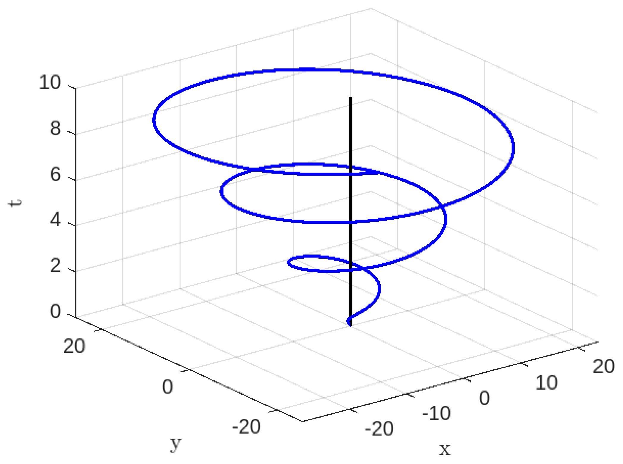
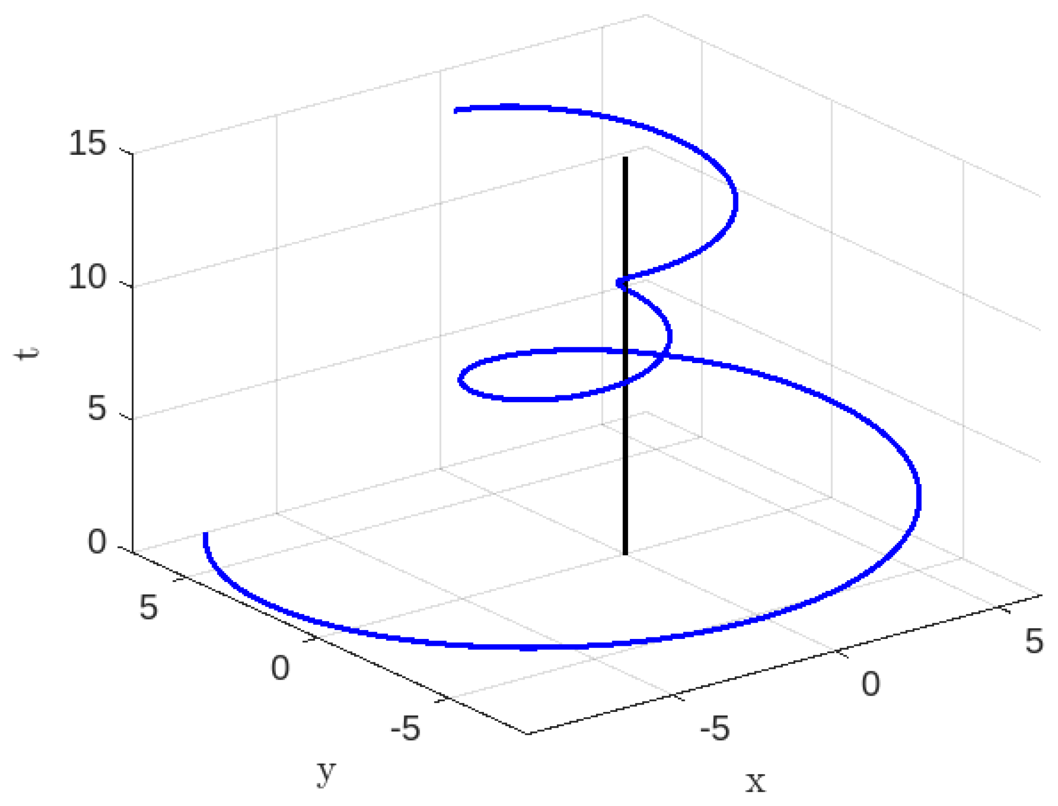
Hence, Equations (47) and (48) demonstrate the possibility of tracing several non-radial time-like geodesics for varying values of under the condition . As a result, a particle starts its journey from when and and will approach to singularity when and , and it will leave the singularity when . Given that , it follows that the values of and are finite for all finite values of and . Also, since , the value of is finite. By using Equations (47) and (48), we have plotted two non-radial time-like geodesics for and , each corresponding to distinct values of and . These geodesics are depicted in Figure 1 and Figure 2, respectively. To plot the geodesics in these diagrams, we have converted the coordinate system from polar coordinates to Cartesian coordinates . It should be noted that there exist central singularities for both the conventional generalized Vaidya spacetime [30,31] and the generalized K-essence Vaidya spacetime [37,38], meaning that both and . However, a singularity is typically defined as only . In this case, we may see that the particle’s track will allow a future observer to watch the particle reach at a specific time and escape the singularity. These phenomena are discussed in the Conclusions.
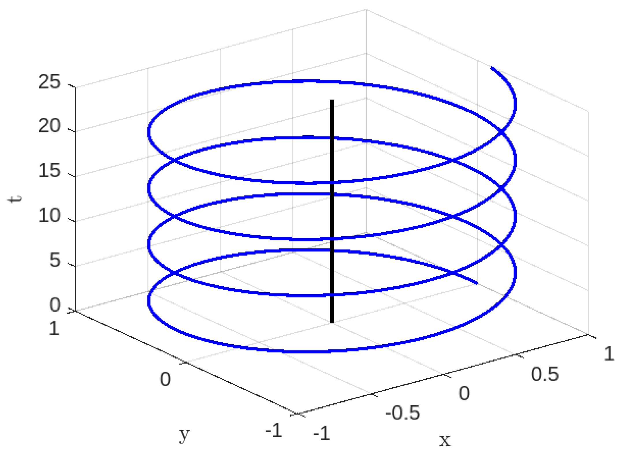
For circular orbits, Equations (38) and (39) can be employed. For a given value of , the corresponding values are and . Thus, there is only a single non-radial time-like circular orbit with a radius of for , as seen in Figure 3, when and . In this regard, it is worth noting that Ishihara et al. [76] have demonstrated that a spacetime that varies with time can possess both an event horizon and a possibility for quasicircular orbits in a different context.
Case–B: To calculate the real solutions of Equation (35) for the purpose of analyzing non-radial time-like geodesics, we assume that . So that Equation (35) can be written as
where
and is an integration constant.
Equation (54) demonstrates that there are two non-radial time-like geodesics that may be followed for any finite value of .
Let a particle start its journey from in the path at time , then Equation (56) yields
Similarly, as before, let us consider a particle that begins its trajectory at along the path (58) at time and eventually approaches singularity at . By analyzing Equations (58) and (59), we may derive the following results:
where and
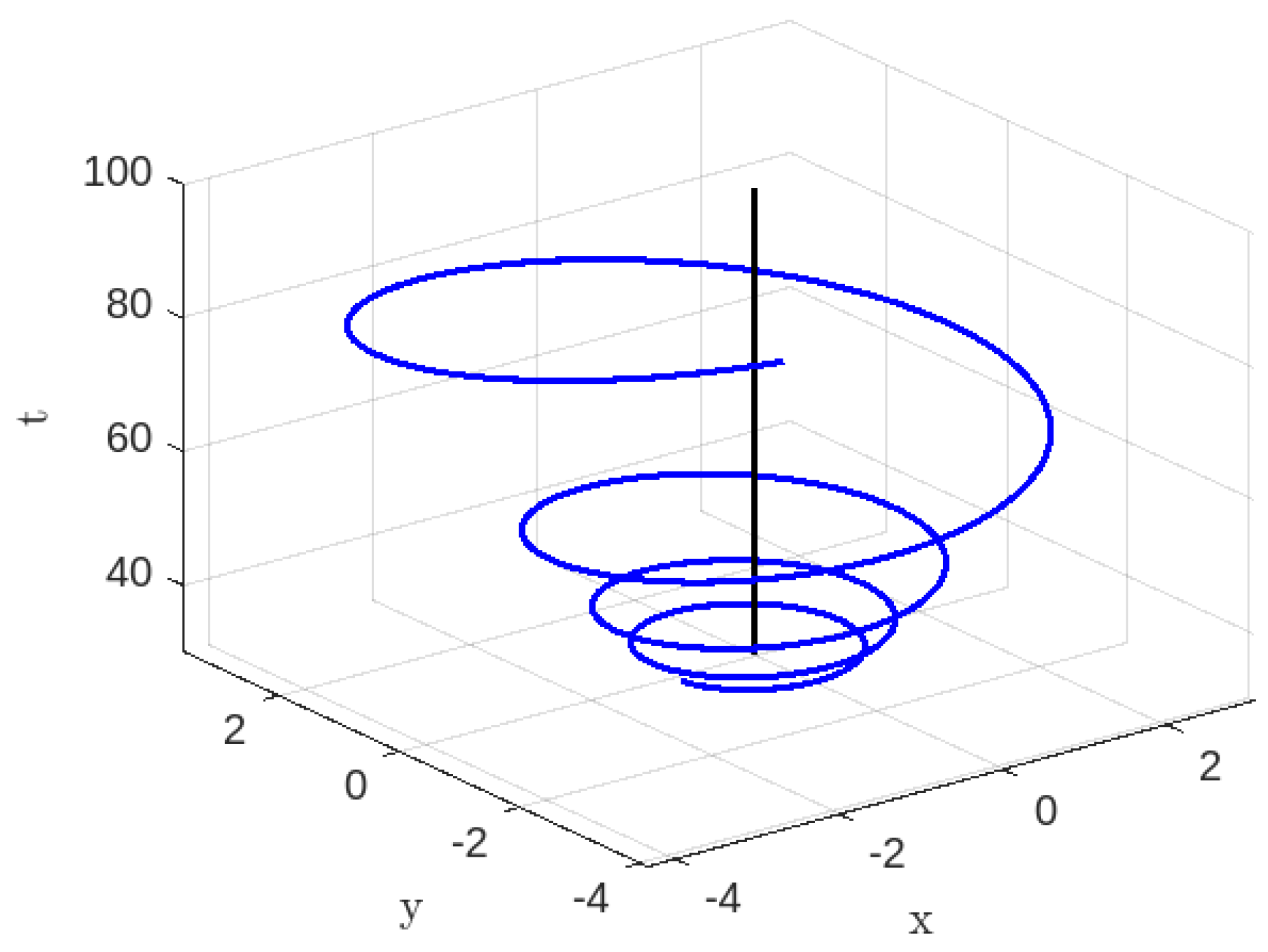
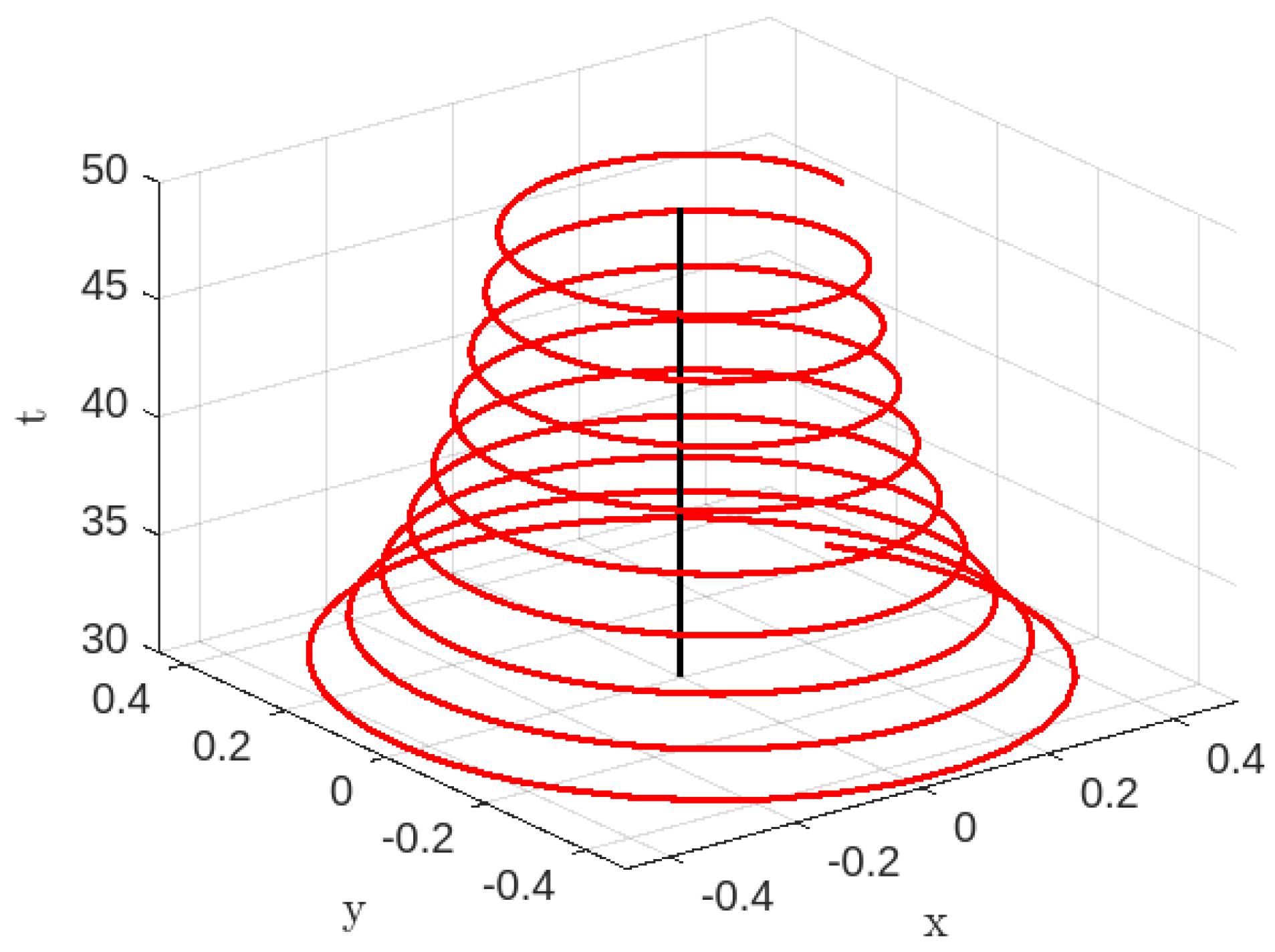
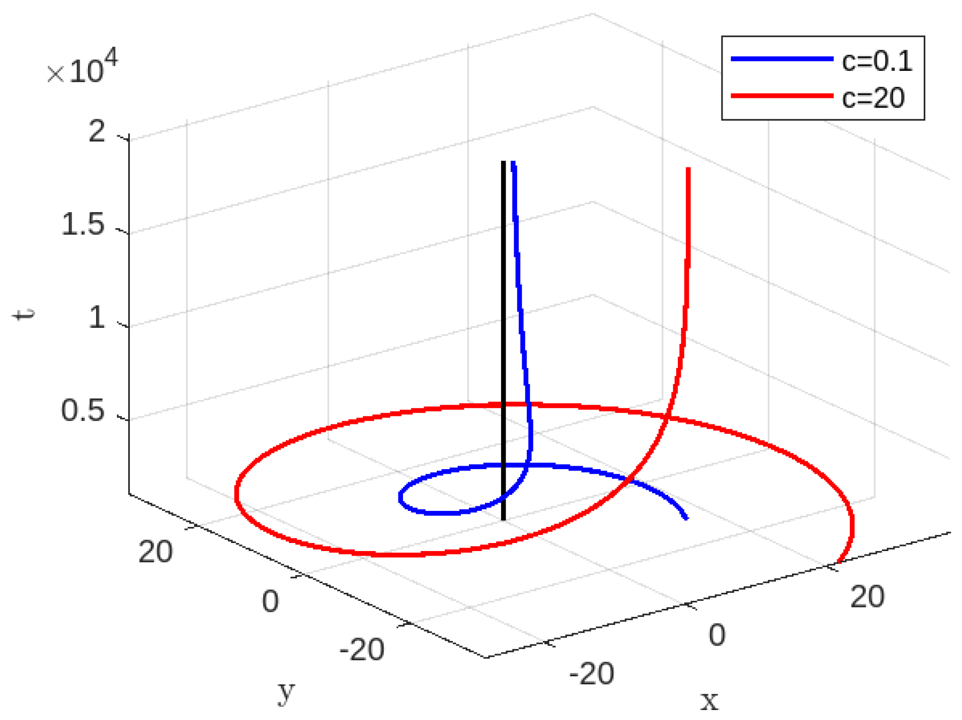
Therefore, Equations (56)–(59) demonstrate the possibility of tracking several non-radial time-like geodesics for distinct values of c given that . Hence, for path (56), a particle starts its journey from when and , and approach when and , and it will leave the singularity when . Also, for path (58), a particle starts its journey from when and , and will arrive at the singularity when and , and it will leave the singularity when . Since and , then for any finite values of , , A, and B, the values of and are also finite. Using Equations (56)–(59), for , , and , we have traced two non-radial time-like for in Figure 4 and also for in Figure 5.
3.1.2. Null Geodesics for Case-I
In this subsection, we want to elucidate the null geodesic behavior of the generalized K-essence Vaidya spacetime, as described by Equation (13) and the mass function given by Equation (27). We assume that . For this study, Equations (33) and (34) reduce to
In order to track the radial geodesics, we assume that a particle with zero angular momentum () begins its motion from a state of rest at a distance of and time , such that the rate of change in r with respect to t is zero (). Thus, based on Equation (32), the value of may be determined as . Clearly, at , we have . Furthermore, according to Equation (70),
where is an integration constant.
At , we obtain
so that
Assuming that the particle reaches the singularity () at a specific time , we determine
Now, we will examine the characteristics of non-radial () geodesics inside the framework of null geodesics in the given spacetime (13), which is governed by the particular mass function (27). The requirement for the existence of real roots of Equation (35) under the assumption that is that . Now, we discuss the following two cases:
Let a particle start its journey from at time ; then, from (76)
It is evident that the inequality is true, and we also have the condition so that
then, Equations (76) and (77) transform to
If we consider that the particle reaches the singularity at time , then from (80) we have
where and .
Therefore, Equations (76) and (77) demonstrate that we may track several non-radial null geodesics for varying values of in the case of . Hence, a particle starts its trajectory at a distance of when and , and will arrive at the singularity when and , and it will leave the singularity when . Given that , it follows that both and are finite for any finite values of and . Also, since , the value of is finite. By using Equations (76) and (77), we have plotted two non-radial time-like geodesics for and , with two distinct values of , namely, and . These geodesics are depicted in Figure 7 and Figure 8, respectively.
Now, for the null circular orbits, using Equations (38) and (39) for , we have and . Therefore, there is only one non-radial null circular orbit of the radius L which can be traced for , as shown in Figure 9 for and .
Equation (83) demonstrates the existence of two non-radial null geodesics that may be followed for any finite value of . Equation (83) is of the same form as (54) in the context of time-like geodesics, but with different constants. Therefore, based on this closeness, we may infer Equations (77) and (83) as
Also,
Let a particle start its journey from in path (85) or (87) at time ; then, from Equation (85), we have
Therefore, we have
and also
If we consider that the particle approaches the singularity at time along path (85) or (87), then we may deduce from Equation (93)
and from (95)
where , , , and .
As the outcome of Equations (85)–(88), we may trace distinct non-radial null geodesics for different values of when . As a result, given the path (85), a particle begins its journey from when and and approaches singularity when and , and it will leave from the singularity when .
Also, for path (87), a particle starts its journey from when and and will approaches singularity when and , and it will leave the singularity when .
Since and , then for any finite values of , , A and B, the values of and are also finite.
3.2. Case-II:
In this part, we consider the generalized K-essence Vaidya mass function (14) with the assumption (26) as
where we take the usual generalized Vaidya mass function , i.e., is a linear function of t [35,36,78] and is a positive constant. In this case, the radii of the dynamical horizons are and (see Appendix A).
From the above mass function (99), we have
where we redefine the first derivative of the given mass function with respect to time as .
Following the same procedure as for Case-I, and using Equations (20)–(25) and (28), and again assuming the comoving plane (), we obtain
Again, continuing the similar procedure as for Case-I, we found the following relations:
Again, proceeding on as before, we have another solution from Equations (103) and (104):
provided and from Equation (24), we obtain
Under this situation, it is evident that the radial part, as indicated by (106), exhibits time dependence. This characteristic is expected in any generalized Vaidya spacetime [30,31,37], given that the background generalized Vaidya mass function is defined as .
3.2.1. Time-like Geodesics for Case-II
In this subsection, we analyze the behavior of time-like geodesics in the generalized K-essence Vaidya spacetime, as described by Equation (13) with the mass function given by Equation (99). For the sake of this investigation, we assume .
Following from the previous analysis for Case-I, we will now focus on tracking the radial geodesics. Specifically, we examine a particle with zero angular momentum () that begins its motion from a state of rest at a distance and time , so that
In this case, at , we also have , which is the same type of condition as in the first Case-I, and using Equation (40), we obtain
Similarly, if the particle approaches the singularity () at time , the same type of consideration applies; we obtain
provided , where .
When studying non-radial time-like geodesics, we obtain the same expression as Equation (35), but with a different value for the parameter D (). In order to trace the geodesics, it is necessary to satisfy the given requirement
In this non-radial study, the scenario where cannot be taken into consideration. This is because if , then , resulting in a constant value for time. As a result, the spacetime is not like the generalized K-essence Vaidya type. So, in this non-radial time-like geodesic investigation, we only look into , ensuring that the spacetime is time-dependent, which is an essential characteristic of both the normal Vaidya spacetime and the generalized K-essence Vaidya spacetime. As before, we solve Equation (35) for , where , and we obtain
where
Clearly, Equation (114) shows that there are two non-radial time-like geodesics that can be traced for any finite value of . Therefore, we have two non-radial time-like geodesics, either
or
Let a particle start its journey from in path (117) at time ; we have
If we assume that the particle reaches the singularity at time along path (117), then we can deduce from Equation (123) the following:
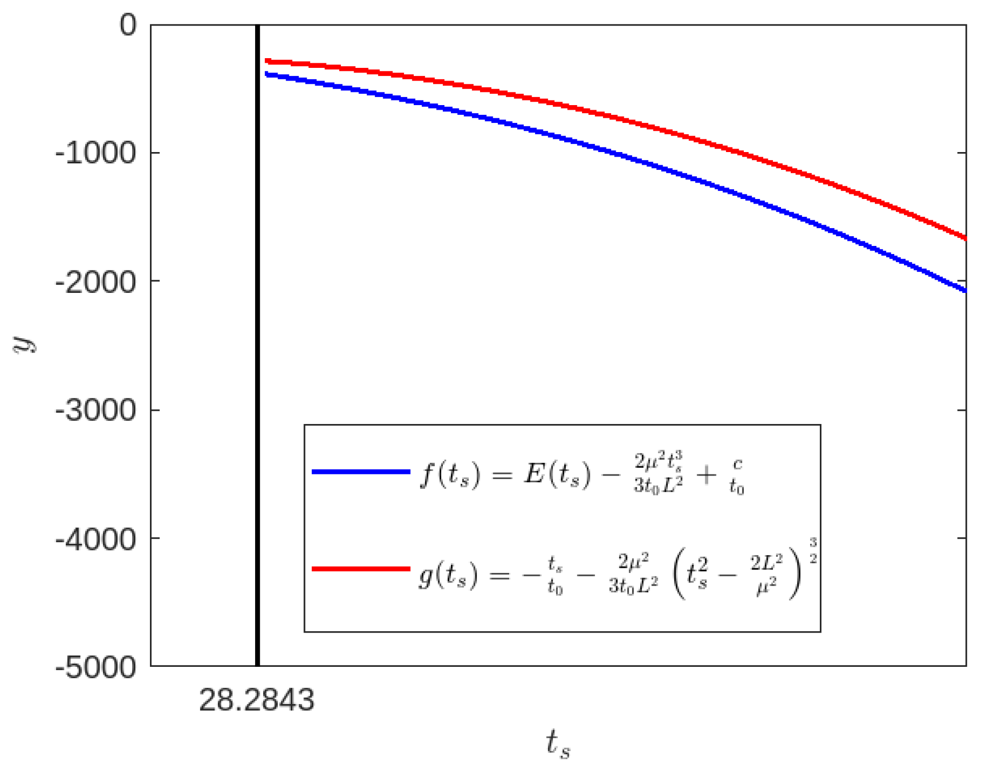
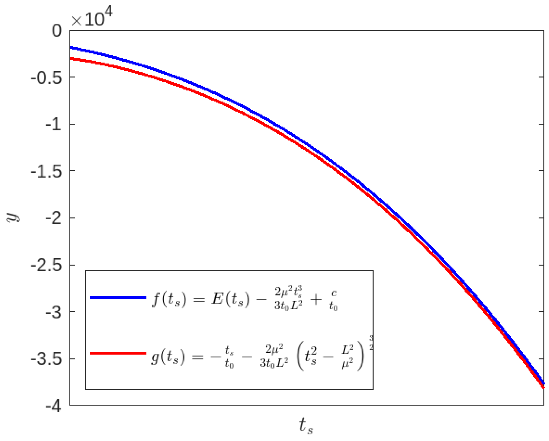
In this scenario, the precise expression for cannot be determined due to the presence of a distinct mass function (99). However, an expression for the transcendental Equation (116) is available, allowing for numerical and graphical analysis to obtain the finite time for any given values of and L. Now, let and . Then, the only possibility for a finite value of is if and only if .
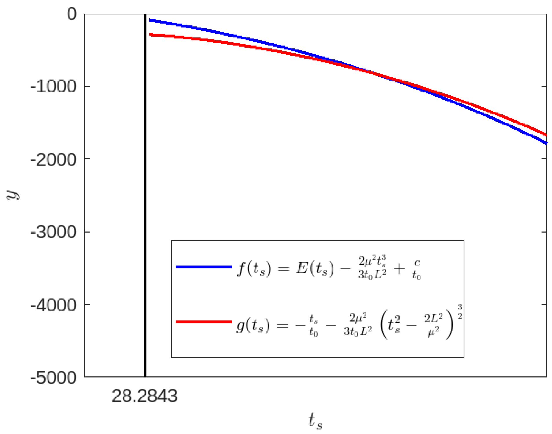
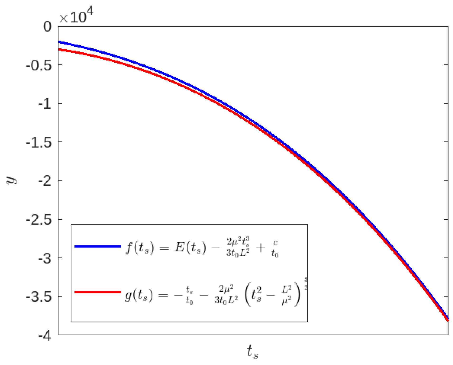
To start with let us consider and , then . Let , and then from (115), . Now, if we consider , then for , and , and also for , and by using (121) and (122). Figure 13 shows that for Equation (126) has no solution for since the curves and do not intersect each other. So, for , the particle which starts from at time will never reach the singularity, as shown in Figure 14 (blue-line) using Equations (117) and (118). However, for , Figure 15 shows that it has a solution for since the curves and intersect each other. For , the particle initially located at at time will eventually reach the singularity () at time , as depicted by the red-line in Figure 14. The particle will then depart from the singularity (), which is shown graphically using Equations (117) and (118).
Again, if we consider a particle starts its journey from in path (119) at time , we have
Once more, assuming it is possible, let us contemplate the scenario in which the particle moves towards the singularity at time along trajectory (119). Consequently, based on Equation (129), we may establish the following relation:
Once again, this equation is transcendental, meaning it can be analyzed numerically and in pictures for any finite values of and L. Now, let and . Then, the only possibility for a finite value of is if and only if .
To start with, let us consider and , then . Again, let and then, from (116), . Now, if we consider , then for , and , and also for , and by using (127) and (131). Now, Figure 16 demonstrates that when , Equation (132) does not have a solution for because the curves and do not cross. So, for , the particle which starts from at time will never reach the singularity as shown in Figure 17 (blue-line) using Equations (119) and (120). However, Figure 18 shows that when , Equation (132) has a solution for since the curves and intersect. For a value of equal to 30, the particle begins at at a time greater than 28.2843. It will eventually reach the singularity at at time , as depicted by the red-line in Figure 17. The particle will then depart from the location , which can be determined from Figure 17 using Equations (119) and (120).
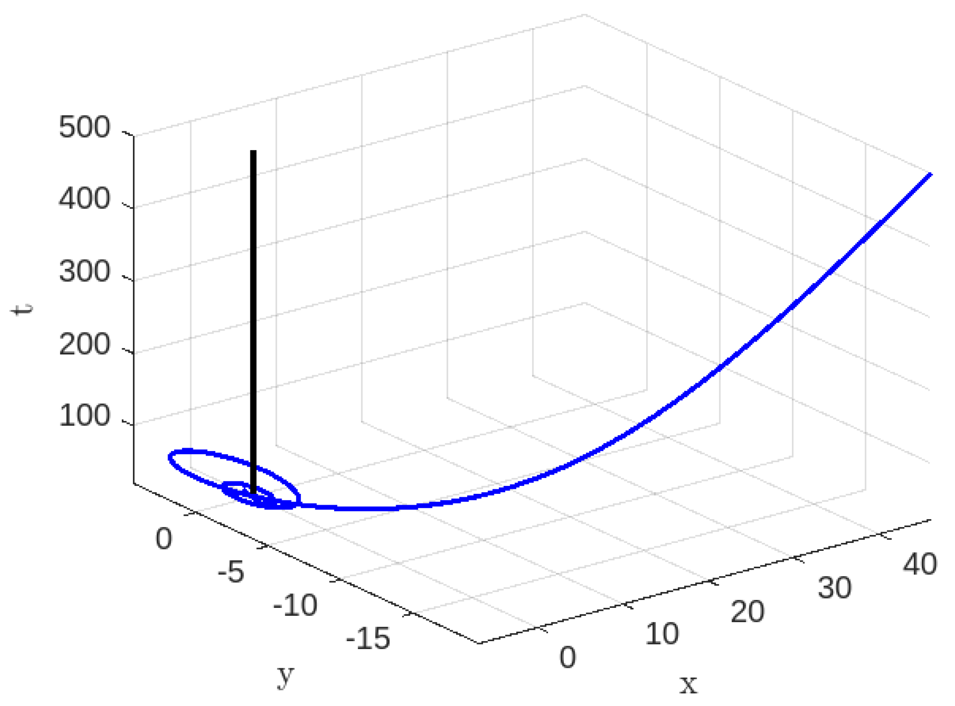
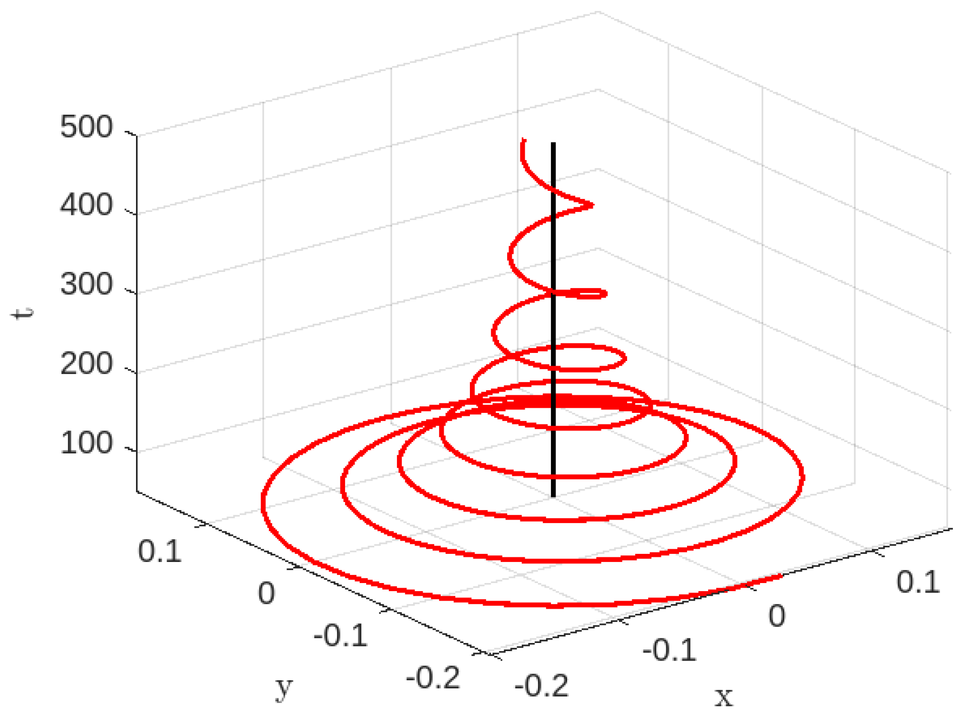
Now, we recall Equations (106) and (107), and for we have and the corresponding . Therefore, two non-radial time-like geodesics can be traced for , as shown in Figure 19 and Figure 20 for and . Figure 19 shows that the orbit starts from a finite distance from the singularity () at time and then departs to infinity since for a large t, and Figure 20 shows that the orbit starts from a finite distance from the singularity at time and then gradually plunges to singularity. Assuming as our reference point, we observe from Figure 19 that the particle trajectory moves away from this reference point. Similarly, from Figure 20 we see that the particle trajectory moves towards from the reference point. This phenomenon again indicates the potential existence of a membrane-like wormhole or a quantum tunneling effect. It is also mentioned that the path of the particle trajectories of the above two scenarios (Figure 19 and Figure 20) are quasicircular [76].
3.2.2. Null Geodesics for Case-II
Within this part, we study the characteristics of both radial () and non-radial () null geodesics in the generalized K-essence Vaidya spacetime (13) with the specific mass function (99).
By tracing the radial null geodesic using the same reasoning as previously, we obtain the identical value of as stated in Equation (108). In this case, at , we also have . Continuing similarly as before, we have
Again, we are able to calculate the time for a particle approaching to singularity ; we obtain
To trace the characteristics of non-radial () null geodesics for the given spacetime (13) through Equation (35) we consider (). Similarly, we exclude the situation when due to the aforementioned rationale for non-radial time-like geodesics. Therefore, when , Equation (35) can be written as
where
Now, Equation (135) indicates the existence of two non-radial null geodesics that may be followed for any finite value of . Proceeding as before, we have
Again, we consider a particle that starts its journey from in path (138) at time ; we obtain
For this scenario, the condition imposed on the particle trajectory is as follows:
since and .
If it is achievable, let us assume that the particle travels along path (138) and reaches the singularity at time . Then, from Equation (144) we obtain
Again, this is also a transcendental equation and it can be analyzed numerically and graphically for any finite value of and L. As before, let and . Then, the only possibility for a finite value of is if and only if . To start with let us consider and , then . Let , then from (136), . Now, if we consider , then for , and , and also for , and by using (142) and (144). Again, Figure 21 and Figure 22 show that for and , Equation (147) does not have a solution for finite since the curves and do not intersect each other. From Equations (138) and (139), we obtain and , so that for large t, we have and . So there is no way to trace any null geodesics for non-zero values of like and , as shown in Figure 23 using Equations (144) and (145). But if we take , a particle starts its journey from and , it finally plunges to the singularity, as shown in Figure 24.
Similar to the previous example, if we look at a particle that begins its journey from in the path described in Equation (140) at time , we obtain the following relations with the same type of meaning from Equations (140), (141) and (137):
Again, as before, Equation (153) is a transcendental equation, so it can be analyzed numerically and graphically for any finite value of and L. Now, let and . Then, the only possibility for a finite value of is if and only if .
To start with let us consider and , then . Let , then from (137), . Now, if we consider , then for , and , and also for , and by using (140) and (141). Figure 25 shows that for , Equation (153) has a solution for since the curves and intersect each other. Also, Figure 26 shows that for , Equation (153) has a solution for since the curves and intersect each other. So, for and , the particle which starts from at time will reach the singularity () at , as shown in Figure 27 using Equations (140) and (141).
Lastly, from Equations (106) and (107), for , we have and the corresponding . Therefore, two non-radial null geodesics can be traced for , as shown in Figure 28 and Figure 29 for and . Figure 28 shows that the orbit starts from a finite distance from the singularity at time and then departs to infinity, since for large t, and Figure 29 shows that the orbit starts from a finite distance from the singularity at time and then gradually plunges to singularity. By analyzing Figure 28 and Figure 29, we can identify a recurrence of the previously observed phenomena, namely, the indication of a probable possibility of a membrane-like wormhole or a quantum tunneling effect.
4. Discussion and Conclusions
In the present investigation, we have traced time-like geodesics and null geodesics for two different K-essence Vaidya mass functions and on equatorial plane by using Euler–Lagrange equations. For both the cases, we observe that can be written in terms of the energy . We have seen that for the radial time-like and radial null geodesics for both the K-essence Vaidya masses, a particle having zero angular momentum starting from a finite distance takes a finite time to reach the singularity () but not in the central singularity, where both the time and space approach to zero, i.e., . For the first K-essence Vaidya mass function, there are two types of families for the time-like case that can be traced, one for and the other for , and similarly for the null case one for and the other for . But a bit of difference was observed for the second K-essence Vaidya mass function. There exists only one type of family for the time-like case when and for the null case . For all the above-mentioned cases, for different finite value of arbitrary constants c, we have traced different kinds of orbits for both the generalized K-essence Vaidya mass function, and the conclusions are as follows.
Based on Figure 1, it may be inferred that a future observer will observe the particle approaching to the singularity within a finite amount of time, as previously stated. According to Figure 2, Figure 3, Figure 4 and Figure 5 it is evident that a future observer can watch the particle reaching the singularity within a finite period and thereafter departing from it. Based on the information provided in Figure 1, Figure 2, Figure 3, Figure 4 and Figure 5, for non-radial time-like geodesics of the generalized K-essence Vaidya spacetime (13) with the first mass function (17) or (27), it can be inferred that there is a worry with the presence of a central singularity (where both r and t approach to 0). It is evident that the central singularity in the generalized Vaidya spacetime is defined by the limits and , as shown in [19,30,32,33,38]. However, based on our analysis of the given data presented in Figure 1, Figure 2, Figure 3, Figure 4 and Figure 5, we may conclude that when r approaches zero, t does not tend to zero. This phenomenon is also observed in the non-radial null geodesics with the same mass function but with varying finite time for different situations, as depicted in Figure 7, Figure 8, Figure 9, Figure 10 and Figure 11. These phenomena can be explained as follows: a future observer is expected to see the particle approaching the singularity and then moving away from it for a limited period of time, (53), (64), or (69) (non-radial time-like geodesic) and (82), (97), or (98) (non-radial null geodesic) in different situations. This observation could potentially indicate the presence of a wormhole during the extreme stages of spacetime, specifically black holes and white holes, similar to the concept of the Einstein–Rosen bridge [79,80,81,82,83,84,85,86,87,88,89].
Regarding particles, it is clear that their signature is changed by the singularity. In this interesting scenario, it seems that the presence of a wormhole allows for the possibility of gravitational collapse resulting in either a naked singularity or a black hole and a white hole in the generalized K-essence Vaidya spacetime with the given mass function (27). Based on the analysis of collapsing scenarios in the generalized Vaidya spacetime, it has been established that there can be either a naked singularity or a black hole [30,38]. This is supported by the potential presence of a dynamical horizon, as discussed in [90,91,92,93]. On the other hand, Vertogradov [35] has also addressed the issue and showed the presence of naked singularities as well as white holes within the framework of the usual generalized Vaidya spacetime in a different setting. However, in our case, the results are a bit different as we have already mentioned that there is the possibility of either a naked singularity or a black hole and a white hole. If we look at all the aforementioned figures with a closer view, then it actually reveals the presence of a wormhole situation also in between the black hole and white hole scenarios. But here, the conditions being extremal ( and ), we have a membrane-type wormhole instead of a tunnel as is usually suggested. Alternatively, the previous explanation can also be explained as follows: Given that the particle reaches the point at and then escapes from there within a certain period, it may be possible that a quantum tunneling event occurs at the vicinity of the central singularity. Since there is a finite time at the typical singular region at , it follows that there is likewise a finite probability of escaping the region at . We also have finite times (45) and (75) to approach the singularity for a particle in radial time-like and null geodesic situations. In these instances, it can be possible to compute the probability amplitude for a time-dependent spacetime, such as the generalized K-essence Vaidya geometry (13). It is important to note that Ellis’s recent study [94] has demonstrated that quantum behavior may occur in time-dependent spacetimes, such as the Vaidya geometry, which is based on Hawking’s recent work [95]. However, it is to be noted that the quantum behavior of generalized K-essence Vaidya geometry cannot be discussed under the present purview.
On the other hand, we have the characteristics of the radial and non-radial time-like or null geodesics structures for the case of the second mass function (99). Through an analysis of the radial properties of the time-like and null geodesics, we have determined that the particle ultimately approaches the singularity at within a limited amount of time, as shown by Equations (112) and (134), respectively. To investigate the non-radial geodesics of the specified spacetime (13) with the mass function (99), we have not found a finite expression for time for a particle to reach the singularity at . However, we have obtained a transcendental equation for different possibilities, namely, Equation (126) or (131) for time-like geodesics and Equation (147) or (153) for null geodesics. But from these transcendental equations, we have analyzed the non-radial time-like or null geodesics through numerical and graphical analyses. Based on Figure 13, Figure 14, Figure 15, Figure 16 and Figure 17, our investigation of non-radial Time-like geodesics reveals that when the particle is unable to reach the singularity at (blue-line). This phenomenon may be explained as follows: The presence of a black hole singularity with an event horizon might result in the spectator being unable to perceive the particle’s journey towards the singularity. Based on the aforementioned figures (red-line), it has been observed that when the constant is set to 30, the particle approaches to the singularity at after a finite amount of time and subsequently moves away from it. Here, we also see the occurrence of a wormhole-like physical phenomenon or quantum tunneling effect near the singularity at .
Regarding the non-radial null geodesic characteristics of the aforementioned spacetime and mass function (99), we note that the transcendental Equations (147) and (153) exhibit the same kind of solutions as Equation (135). In this situation also, we are as yet unable to determine the expression for the time it takes to reach the singularity at . After solving the transcendental equations using numerical analysis, we find the graphical solutions through Figure 21, Figure 22, Figure 23, Figure 24, Figure 25, Figure 26 and Figure 27. From Figure 23, we have not found any tracing of the non-radial null geodesic structure for two choices of the constants, viz., and , though it is available for the choice of ; see Figure 24 and Figure 25. No traces of the non-radial null geodesic structure were noticed in Figure 23 for two different values of the constants, namely, and . However, by setting , as seen in Figure 24, it is evident that the particle originates from a specific location and ultimately drops into the singularity. Alternatively, we have explored an additional solution to Equation (135) and its associated Equation (153). We have analyzed the non-radial null geodesic structure and depicted it in Figure 27. In this scenario, we note that for two specific values of the constants, namely, and , the particle begins its trip from a fixed position and eventually reaches the singularity within a limited amount of time. After reaching the singularity, the particle then escapes from it. This once again indicates the presence of a wormhole or the quantum tunneling effect.
We have found that instead of the dynamical horizon, the circular orbits via the event horizons (38) provide alternative solutions for Equations (32) and (33) in the case of the first mass function (27). The corresponding graphical representations of the circular orbits can be observed in Figure 3, Figure 6, Figure 9 and Figure 12. These phenomena can be supported by the study conducted by Ishihara et al. [76] on a time-dependent spacetime in a different setting. On the other hand, for the second mass function (99), Equations (103) and (104) have alternative solutions, which are (106) and (107). By observing solution (106), it is evident that the values of vary with time, a characteristic that is inherent in all forms of generalized Vaidya spacetime. This suggests the possible presence of a dynamical horizon rather than an event horizon, which is seen in the case of the generalized K-essence Vaidya spacetime. Based on solutions (106) and (107), we obtain four plots: Figure 19, Figure 20, Figure 28 and Figure 29. Based on these plots, we observe evidence of the possible presence of a membrane-like wormhole or a quantum tunneling phenomenon, as well as hints of a quasicircular orbit along the particle trajectory.
Therefore, under the aforementioned discussion, we can conclude that in our specific model, we have investigated the existence of a wormhole during the extreme stages of spacetime, specifically black holes and white holes, similar to the concept of the Einstein–Rosen bridge or quantum tunneling effect near the central singularity. This investigation was carried out in the comoving frame for the generalized K-essence Vaidya spacetime using two types of K-essence Vaidya mass functions. It is possible to argue that extra interactions between the K-essence scalar field and the usual gravity are the cause of this occurrence. Furthermore, it should be noted that in our specific scenario, there is no presence of a central singularity, i.e., both r and t approach to zero, which is a need for any form of generalized Vaidya geometry. Usually, the singularity means , at which point geodesics are incomplete. It might be argued that the presence of singularity is uncertain, as has been shown very recently by Kerr [96], where he demonstrates the lack of evidence supporting the existence of singularities within black holes formed by real physical spacetime. In a nutshell, we may state that a physical spacetime does not exhibit geodesic incompleteness. Geodesic completeness relates to the concept that these trajectories should continue endlessly in time inside a well-behaved and physically plausible spacetime. Penrose [97] and Hawking [98] demonstrated that geodesics can be incomplete under specific circumstances, indicating that they may only persist for a finite time before meeting a singularity, a location where the curvature of spacetime becomes indefinitely large. In this context, we may state that in the present investigation our spacetime (13) is geodesically complete under certain perspectives.
At this juncture, we would like to point out that the wormhole geometries given by the present solutions may or may not be traversable. This is because, though K-essence inherently admits dark energy, we have not directly included any exotic component that is essential for forming a wormhole traversable via its throat [99,100,101,102,103,104,105]. But here, we have not used the K-essence model as a dark energy model, rather we have adapted it to a purely gravitational perspective [37,38]. However, in the case of possible quantum tunneling, there is no need of such a type of traversable structure where the quantum field theoretic effect becomes predominant.
Moreover, based on the investigation of the present work, especially the observations in Figure 2, Figure 3, Figure 4 and Figure 5, one may raise the issue of black holes and baby universes [106], and whether there is any possibility of such situations under the generalized K-essence Vaidya spacetime. This obviously draws special attention and can be considered as a potential topic in the near future.
Author Contributions
Conceptualization and writing—original draft preparation, G.M.; writing—original draft preparation, B.M.; writing—review and editing, M.K. and S.R. All authors have read and agreed to the published version of the manuscript.
Funding
G.M. acknowledges the DSTB, Government of West Bengal, India for financial support through Grant Nos. 322(Sanc.)/ST/P/S&T/16G-3/2018 dated 6 March 2019. The research by M.K. was carried out at Southern Federal University with financial support from the Ministry of Science and Higher Education of the Russian Federation (State Contract GZ0110/23-10-IF).
Data Availability Statement
There are no assoiated data with this artile as such no new data were generated or analyzed in support of this research.
Acknowledgments
S.R. is thankful to the Inter-University Centre for Astronomy and Astrophysics (IUCAA), Pune, India, for providing the Visiting Associateship under which a part of this work was carried out. S.R. also acknowledges the facilities under ICARD at CCASS, GLA University, Mathura, India. Additionally, the authors express their gratitude to the referees for providing insightful comments to enhance the quality of the work. Also, all the authors are grateful to P. Panchadhyayee of P.K. College, Contai, West Bengal, India, for fruitful discussions.
Conflicts of Interest
The authors declare no conflict of interest.
Appendix A. Radius of the Dynamical Horizon
To start with, let us consider
and then generalized K-essence Vaidya spacetime (13) can be expressed as
Setting , where is a tortoise coordinate with , i.e.,
where , which implies . Here we have used and . Following [39,40], the null vectors can be written as and and the corresponding expansions of the two null vectors and , and [39,40], are
and
where .
One can note that
and the other null expansion is strictly negative, which are the required conditions for the dynamical horizon [40,90,91,92].
So, we can proceed by using the dynamical horizon equation.
Now, from Equation (A3), we have
Therefore, the dynamical horizon radii are and , where is the solution of the equation when q is a non-negative real number. It is also noted that the Lambert function [77] is a single-valued function.
Detail Derivation
On the other hand, at the dynamical horizon (), we can write
It is important to mention that the procedure for deriving the dynamical horizon differs from our previous work [39], while the outcome is identical.
References
- Chandrasekhar, S. The Mathematical Theory of Black Holes; Indian Edition 2010; Oxford University Press: Oxford, UK, 1992. [Google Scholar]
- Cruz, N.; Olivares, M.; Saavedra, J.; Villanueva, J.R. The geodesic structure of the Schwarzschild anti-de Sitter black hole. Class. Quantum Grav. 2005, 22, 1167–1190. [Google Scholar] [CrossRef]
- Berti, E. A Black-Hole Primer: Particles, Waves, Critical Phenomena and Superradiant Instabilities. arXiv 2014, arXiv:1410.4481. [Google Scholar]
- Gibbons, G.W. The Jacobi metric for timelike geodesics in static spacetimes. Class. Quantum Grav. 2016, 33, 025004. [Google Scholar] [CrossRef]
- Chanda, S.; Gibbons, G.W.; Guha, P. Jacobi-Maupertuis-Eisenhart metric and geodesic flows. J. Math. Phys. 2017, 58, 032503. [Google Scholar] [CrossRef]
- Eisenhart, L.P. Dynamical Trajectories and Geodesics. Ann. Math. Second Ser. 1928, 30, 591–606. [Google Scholar] [CrossRef]
- Duval, C.; Burdet, G.; Künzle, H.P.; Perrin, M. Bargmann structures and Newton-Cartan theory. Phy. Rev. D 1985, 31, 1841. [Google Scholar] [CrossRef]
- Majumder, B.; Manna, G.; Das, A. Time-like geodesic structure for the emergent Barriola–Vilenkin type spacetime. Class. Quantum Grav. 2020, 37, 115002. [Google Scholar] [CrossRef]
- Barriola, M.; Vilenkin, A. Gravitational field of a global monopole. Phys. Rev. Lett. 1989, 63, 341. [Google Scholar] [CrossRef]
- Gangopadhyay, D.; Manna, G. The Hawking temperature in the context of dark energy. Europhys. Lett. 2012, 100, 49001. [Google Scholar] [CrossRef]
- Vaidya, P.C. The gravitational field of a radiating star. Proc. Indian Acad. Sci. Sect. A 1951, 33, 264. [Google Scholar] [CrossRef]
- Joshi, P.S. Gravitational collapse: The story so far. Pramana J. Phys. 2000, 55, 529. [Google Scholar] [CrossRef]
- Joshi, P.S. Global Aspects in Gravitation and Cosmology; Clarendon: Oxford, UK, 1993. [Google Scholar]
- Joshi, P.S.; Dwivedi, I.H. Naked singularities in spherically symmetric inhomogeneous Tolman-Bondi dust cloud collapse. Phys. Rev. D 1993, 47, 5357. [Google Scholar] [CrossRef] [PubMed]
- Joshi, P.S.; Dwivedi, I.H. The structure of naked singularity in self-similar gravitational collapse: II. Commun. Math. Phys. 1992, 146, 333. [Google Scholar] [CrossRef]
- Joshi, P.S.; Singh, T.P. Role of initial data in the gravitational collapse of inhomogeneous dust. Phys. Rev. D 1995, 51, 6778. [Google Scholar] [CrossRef]
- Oppenheimer, J.R.; Snyder, H. On Continued Gravitational Contraction. Phys. Rev. 1939, 56, 455. [Google Scholar] [CrossRef]
- Malafarina, D. Classical Collapse to Black Holes and Quantum Bounces: A Review. Universe 2017, 3, 48. [Google Scholar] [CrossRef]
- Dwivedi, I.H.; Joshi, P.S. On the nature of naked singularities in Vaidya spacetimes: II. Class. Quantum Gravit. 1989, 6, 1599. [Google Scholar] [CrossRef]
- Papapetrou, A. A Random Walk in Relativity and Cosmology; Dadhich, N., Rao, J.K., Narlikar, J.V., Vishveshwara, C.V., Eds.; John Wiley and Sons: New York, NY, USA, 1985; p. 184. [Google Scholar]
- Penrose, R. Gravitational Collapse: The Role of General Relativity. Riv. Nuovo Cim. 1969, 1, 252. Available online: https://ui.adsabs.harvard.edu/abs/1969NCimR...1..252P/abstract (accessed on 3 April 2023).
- Penrose, R. “Golden Oldie”: Gravitational Collapse: The Role of General Relativity. Gen. Rel. Grav. 2002, 34, 1141. [Google Scholar] [CrossRef]
- Vertogradov, V. Gravitational collapse of Vaidya spacetime. Int. J. Mod. Phys. Conf. Ser. 2016, 41, 1660124. [Google Scholar] [CrossRef]
- Vaidya, P.C. Nonstatic Solutions of Einstein’s Field Equations for Spheres of Fluids Radiating Energy. Phys. Rev. 1951, 83, 1. [Google Scholar] [CrossRef]
- Vaidya, P.C.; Pandya, I.M. Gravitational Field of a Radiating Spheroid. Prog. Theor. Phys. 1966, 35, 1. [Google Scholar] [CrossRef]
- Vaidya, P.C. Nonstatic Analogs of Schwarzschild’s Interior Solution in General Relativity. Phys. Rev. 1968, 174, 5. [Google Scholar] [CrossRef]
- Vaidya, P.C. An Analytical Solution for Gravitational Collapse with Radiation. APJ 1966, 144, 943. [Google Scholar] [CrossRef]
- Vaidya, P.C. The External Field of a Radiating Star in General Relativity. Gen. Rel. Grav. 1999, 31, 119. [Google Scholar] [CrossRef]
- Griffiths, J.B.; Podolsky, J. Exact Space-Times in Einstein’s General Relativity; Cambridge Monographs on Mathematical Physics; Cambridge University Press: Cambridge, UK, 2009. [Google Scholar]
- Husain, V. Exact solutions for null fluid collapse. Phys. Rev. D 1996, 53, 4. [Google Scholar] [CrossRef]
- Wang, A.; Wu, Y. LETTER: Generalized Vaidya Solutions. Gen. Rel. Grav. 1999, 31, 107. Available online: https://www.springer.com/journal/10714 (accessed on 3 April 2023). [CrossRef]
- Mkenyeleye, M.D.; Goswami, R.; Maharaj, S.D. Collapsing spherical stars in f(R) gravity. Phys. Rev. D 2014, 90, 064034. [Google Scholar] [CrossRef]
- Patil, K.D. Gravitational collapse in higher-dimensional charged-Vaidya space-time. Pramana—J. Phys. 2003, 60, 423. [Google Scholar] [CrossRef]
- Coudray, A.; Nicolas, J.P. Geometry of Vaidya spacetimes. Gen. Rel. Gravit. 2021, 53, 73. [Google Scholar] [CrossRef]
- Vertogradov, V. The structure of the generalized Vaidya space–time containing the eternal naked singularity. Int. J. Mod. Phys. A 2022, 37, 2250185. [Google Scholar] [CrossRef]
- Solanki, J.; Perlick, V. Photon sphere and shadow of a time-dependent black hole described by a Vaidya metric. Phys. Rev. D 2022, 105, 064056. [Google Scholar] [CrossRef]
- Manna, G.; Majumdar, P.; Majumder, B. k-essence emergent spacetime as a generalized Vaidya geometry. Phys. Rev. D 2020, 101, 124034. [Google Scholar] [CrossRef]
- Manna, G. Gravitational collapse for the K-essence emergent Vaidya spacetime. Eur. Phys. J. C 2020, 80, 813. [Google Scholar] [CrossRef]
- Majumder, B.; Ray, S.; Manna, G. Evaporation of Dynamical Horizon with the Hawking Temperature in the K-essence Emergent Vaidya Spacetime. Fortschr. Phys. 2023, 71, 2300133. [Google Scholar] [CrossRef]
- Sawayama, S. Evaporating dynamical horizon with the Hawking effect in Vaidya spacetime. Phys. Rev. D 2006, 73, 064024. [Google Scholar] [CrossRef]
- Armendariz-Picon, C.; Damour, T.; Mukhanov, V. k-Inflation. Phys. Lett. B 1999, 458, 209–218. [Google Scholar] [CrossRef]
- Armendariz-Picon, C.; Mukhanov, V.; Steinhardt, P.J. Dynamical Solution to the Problem of a Small Cosmological Constant and Late-Time Cosmic Acceleration. Phys. Rev. Lett. 2000, 85, 4438. [Google Scholar] [CrossRef]
- Armendariz-Picon, C.; Mukhanov, V.; Steinhardt, P.J. Essentials of k-essence. Phys. Rev. D 2001, 63, 103510. [Google Scholar] [CrossRef]
- Visser, M.; Barcelo, C.; Liberati, S. Analogue Models of and for Gravity. Gen. Rel. Grav. 2002, 34, 1719. [Google Scholar] [CrossRef]
- Scherrer, R.J. Purely Kinetic k Essence as Unified Dark Matter. Phys. Rev. Lett. 2004, 93, 011301. [Google Scholar] [CrossRef]
- Chimento, L.P. Extended tachyon field, Chaplygin gas, and solvable k-essence cosmologies. Phys. Rev. D 2004, 69, 123517. [Google Scholar] [CrossRef]
- Vikman, A. K-Essence: Cosmology, Causality and Emergent Geometry. Doctoral Dissertation, der Ludwig-Maximilians-Universitat Munchen, Munchen, Germany, 2007. [Google Scholar]
- Babichev, E.; Mukhanov, V.; Vikman, A. k-Essence, superluminal propagation, causality and emergent geometry. J. High Energy Phys. 2008, 2, 101. [Google Scholar] [CrossRef]
- Babichev, E.; Mukhanov, V.; Vikman, A. Looking beyond the horizon. Looking beyond the Horizon. arXiv 2007, arXiv:0704.3301. [Google Scholar]
- Chimento, L.P. Internal space structure generalization of the quintom cosmological scenario. Phys. Rev. D 2009, 79, 043502. [Google Scholar] [CrossRef]
- Singh, T.; Chaubey, R.; Singh, A. k-essence cosmologies in Kantowski–Sachs and Bianchi space–times. Can. J. Phys. 2015, 93, 1319. [Google Scholar] [CrossRef]
- Singh, A.; Raushan, R.; Chaubey, R.; Mandal, S.; Mishra, K.C. Lagrangian formulation and implications of barotropic fluid cosmologies. Int. J. Geom. Meth. Mod. Phys. 2022, 19, 2250107. [Google Scholar] [CrossRef]
- Tian, S.X.; Zhu, Z.H. Early dark energy in k-essence. Phys. Rev. D 2021, 103, 043518. [Google Scholar] [CrossRef]
- Myrzakulov, R.; Sebastiani, L. k-Essence Non-Minimally Coupled with Gauss–Bonnet Invariant for Inflation. Symmetry 2016, 8, 57. [Google Scholar] [CrossRef]
- Sen, A.A.; Devi, N.C. Cosmology with non-minimally coupled k-field. Gen. Relativ. Gravit. 2010, 42, 821. [Google Scholar] [CrossRef]
- Chatterjee, A.; Hussain, S.; Bhattacharya, K. Dynamical stability of the k-essence field interacting nonminimally with a perfect fluid. Phys. Rev. D 2021, 104, 103505. [Google Scholar] [CrossRef]
- Velten, H.E.S.; Vom Marttens, R.F.; Zimdahl, W. Aspects of the cosmological “coincidence problem”. Eur. Phys. J. C 2014, 74, 3160. [Google Scholar] [CrossRef]
- Erickson, J.K.; Caldwell, R.R.; Steinhardt, P.J.; Armendariz-Picon, C.; Mukhanov, V. Measuring the Speed of Sound of Quintessence. Phys. Rev. Lett. 2002, 88, 121301. [Google Scholar] [CrossRef] [PubMed]
- DeDeo, S.; Caldwell, R.R.; Steinhardt, P.J. Effects of the Sound Speed of Quintessence on the Microwave Background and Large Scale Structure. Phys. Rev. D 2003, 67, 103509. [Google Scholar] [CrossRef]
- Bean, R.; Dore, O. Probing dark energy perturbations: The dark energy equation of state and speed of sound as measured by WMAP. Phys. Rev. D 2004, 69, 083503. [Google Scholar] [CrossRef]
- Manna, G.; Gangopadhyay, D. The Hawking temperature in the context of dark energy for Reissner–Nordstrom and Kerr background. Eur. Phys. J. C 2014, 74, 2811. [Google Scholar] [CrossRef]
- Manna, G.; Majumder, B. The Hawking temperature in the context of dark energy for Kerr–Newman and Kerr–Newman–AdS backgrounds. Eur. Phys. J. C 2019, 79, 553. [Google Scholar] [CrossRef]
- Manna, G.; Majumder, B.; Das, A. Quantum corrections to the accretion onto a Schwarzschild black hole in the background of quintessence. Eur. Phys. J. Plus 2020, 135, 107. [Google Scholar] [CrossRef]
- Manna, G.; Panda, A.; Karmakar, A.; Ray, S. -gravity in the context of dark energy with power law expansion and energy conditions*. Chin. Phys. C 2023, 47, 025101. [Google Scholar] [CrossRef]
- Ray, S.; Panda, A.; Majumder, B.; Islam, M.R.; Manna, G. Collapsing scenario for the k-essence emergent generalized Vaidya spacetime in the context of massive gravity’s rainbow. Chin. Phys. C 2022, 46, 125103. [Google Scholar] [CrossRef]
- Das, S.; Panda, A.; Manna, G.; Ray, S. Raychaudhuri Equation in K-essence Geometry: Conditional Singular and Non-Singular Cosmological Models. Fortschr. Phys. 2023, 2023, 2200193. [Google Scholar] [CrossRef]
- Mukohyama, S.; Namba, R.; Watanabe, Y. Is the DBI scalar field as fragile as other k-essence fields? Phys. Rev. D 2016, 94, 023514. [Google Scholar] [CrossRef]
- Born, M.; Infeld, L. Foundations of the new field theory. Proc. R. Soc. Lond. A 1934, 144, 425. [Google Scholar] [CrossRef]
- Heisenberg, W. Production of Meson Showers. Zeit. Phys. 1939, 113, 61. [Google Scholar] [CrossRef]
- Dirac, P.A.M. An extensible model of the electron. Proc. R. Soc. Lond. A 1962, 268, 57. [Google Scholar] [CrossRef]
- Panda, A.; Manna, G.; Ray, S.; Khlopov, M.; Islam, M.R. Gravitational collapse in generalized K-essence emergent Vaidya spacetime via gravity. arXiv 2023, arXiv:2308.13574. [Google Scholar]
- Panda, A.; Das, S.; Manna, G.; Ray, S.; Islam, M.R.; Ranjit, C. gravity in a Non-canonical theory. arXiv 2022, arXiv:2206.14808. [Google Scholar]
- Ade, P.A.R.; Aghanim, N.; Arnaud, M.; Ashdown, M.; Aumont, J.; Baccigalupi, C.; Banday, A.J.; Barreiro, R.B.; Bartolo, N.; Battaner, E.; et al. [Planck Collaboration]. XIV. Dark energy and modified gravity. Astron. Astrophys. 2016, 594, A14. [Google Scholar] [CrossRef]
- Aghanim, N.; Akrami, Y.; Ashdow, M.; Aumont, J.; Baccigalupi, C.; Ballardini, M.; Banday, A.J.; Barreiro, R.B.; Bartolo, N.; Basak, S.; et al. [Planck Collaboration]. VI. Cosmological parameters. Astron. Astrophys. 2020, 641, A6. [Google Scholar] [CrossRef]
- Aghanim, N.; Akrami, Y.; Arroja, F.; Ashdow, M.; Aumon, J.; Baccigalupi, C.; Ballardini, M.; Banday, A.J.; Barreir, R.B.; Bartolo, N.; et al. [Planck Collaboration]. I. Overview and the cosmological legacy of Planck. Astron. Astrophys. 2020, 641, A1. [Google Scholar] [CrossRef]
- Ishihara, H.; Kimura, M.; Matsuno, K. Charged black strings in a five-dimensional Kasner universe. Phys. Rev. D 2016, 93, 024037. [Google Scholar] [CrossRef]
- Corless, R.M.; Gonnet, G.H.; Hare, D.E.G.; Jeffrey, D.J.; Knuth, D.E. On the LambertW function. Adv. Comp. Math. 1996, 5, 329. [Google Scholar] [CrossRef]
- Blau, M. Lecture Notes on General Relativity. 8 October 2022. Available online: http://www.blau.itp.unibe.ch/GRLecturenotes.html (accessed on 3 April 2023).
- Einstein, A.; Rosen, N. The Particle Problem in the General Theory of Relativity. Phys. Rev. 1935, 48, 73. [Google Scholar] [CrossRef]
- Fuller, R.W.; Wheeler, J.A. Causality and Multiply Connected Space-Time. Phys. Rev. 1962, 128, 919. [Google Scholar] [CrossRef]
- Ellis, H.G. Ether flow through a drainhole: A particle model in general relativity. J. Math. Phys. 1973, 14, 104. [Google Scholar] [CrossRef]
- Morris, M.S.; Thorne, K.S. Wormholes in spacetime and their use for interstellar travel: A tool for teaching general relativity. Am. J. Phys. 1988, 56, 395. [Google Scholar] [CrossRef]
- Visser, M. Traversable wormholes: Some simple examples. Phys. Rev. D 1989, 39, 3182. [Google Scholar] [CrossRef] [PubMed]
- Hayward, S.A. Wormhole dynamics in spherical symmetry. Phys. Rev. D 2009, 79, 124001. [Google Scholar] [CrossRef]
- Bronnikov, K.A.; Lipatova, L.N.; Novikov, I.D.; Shatskiy, A.A. Example of a stable wormhole in general relativity. Gravit. Cosmol. 2013, 19, 269. [Google Scholar] [CrossRef]
- Garattini, R. Casimir wormholes. Eur. Phys. J. C 2019, 79, 951. [Google Scholar] [CrossRef]
- Mishra, B.; Agrawal, A.S.; Tripathy, S.K.; Ray, S. Wormhole solutions in f(R) gravity. Int. J. Mod. Phys. D 2021, 30, 2150061. [Google Scholar] [CrossRef]
- Mishra, B.; Agrawal, A.S.; Tripathy, S.K.; Ray, S. Traversable wormhole models in f(R) gravity. Int. J. Mod. Phys. A 2022, 37, 2250010. [Google Scholar] [CrossRef]
- Mustafa, G.; Maurya, S.K.; Ray, S. On the Possibility of Generalized Wormhole Formation in the Galactic Halo Due to Dark Matter Using the Observational Data within the Matter Coupling Gravity Formalism. Astrophys. J. 2022, 941, 170. [Google Scholar] [CrossRef]
- Ashtekar, A.; Krishnan, B. Dynamical horizons and their properties. Phys. Rev. D 2003, 68, 104030. [Google Scholar] [CrossRef]
- Ashtekar, A.; Krishnan, B. Dynamical Horizons: Energy, Angular Momentum, Fluxes, and Balance Laws. Phys. Rev. Lett. 2002, 89, 261101. [Google Scholar] [CrossRef]
- Ashtekar, A.; Krishnan, B. Isolated and Dynamical Horizons and Their Applications. Living Rev. Relativ. 2004, 7, 10. [Google Scholar] [CrossRef]
- Hayward, S.A. General laws of black-hole dynamics. Phys. Rev. D 1994, 49, 6467. [Google Scholar] [CrossRef]
- Firouzjaee, J.T.; Ellis, G.F.R. Particle creation rate for dynamical black holes. Eur. Phys. J. C 2016, 76, 620. [Google Scholar] [CrossRef]
- Hawking, S.W.; Perry, M.J.; Strominger, A. Soft Hair on Black Holes. Phys. Rev. Lett. 2016, 116, 231301. [Google Scholar] [CrossRef]
- Kerr, R. Do Black Holes have Singularities? arXiv 2023, arXiv:2312.00841. [Google Scholar] [CrossRef]
- Penrose, R. Gravitational Collapse and Space-Time Singularities. Phys. Rev. Lett. 1965, 14, 57. [Google Scholar] [CrossRef]
- Hawking, S.W. Black holes in general relativity. Commun. Math. Phys. 1972, 25, 152–166. [Google Scholar] [CrossRef]
- Hochberg, D.; Visser, M. Geometric structure of the generic static traversable wormhole throat. Phys. Rev. D 1997, 56, 4745. [Google Scholar] [CrossRef]
- Krasnikov, S. Traversable wormhole. Phys. Rev. D 2000, 62, 084028. [Google Scholar] [CrossRef]
- Matos, T.; Nunez, D. Rotating scalar field wormhole. Class. Quantum Gravit. 2006, 23, 4485. [Google Scholar] [CrossRef]
- Rahaman, F.; Islam, S.; Kuhfittig, P.K.F.; Ray, S. Searching for higher-dimensional wormholes with noncommutative geometry. Phys. Rev. D 2012, 86, 106010. [Google Scholar] [CrossRef]
- Rahaman, F.; Karmakar, S.; Karar, I.; Ray, S. Wormhole inspired by non-commutative geometry. Phys. Lett. B 2015, 746, 73. [Google Scholar] [CrossRef]
- Chew, X.Y.; Kleihaus, B.; Kunz, J. Geometry of spinning Ellis wormholes. Phys. Rev. D 2016, 94, 104031. [Google Scholar] [CrossRef]
- Mustafa, G.; Maurya, S.K.; Ray, S.; Javed, F. Construction of thin-shell around new wormhole solutions via solitonic quantum wave dark matter. Ann. Phys. 2014, 460, 169551. [Google Scholar] [CrossRef]
- Hawking, S. Black Holes and Baby Universes and Other Essays; Bantam Dell Publishing Group: New York, NY, USA, 1993. [Google Scholar]
Figure 1.
Time-like geodesics for , , , and .

Figure 2.
Time-like geodesics for , , , and .

Figure 3.
Circular orbit of time-like geodesics for , , and .

Figure 4.
Time-like geodesics for , , , and . Blue-line for and red-line for .

Figure 5.
Time-like geodesics for , , , and . Blue-line for and red-line for .

Figure 6.
Circular time-like geodesics for , , and . Blue-line for and red-line for .

Figure 7.
Null geodesics for , , , and .

Figure 8.
Null geodesics for , , , and .

Figure 9.
Circular null geodesics for , , and .

Figure 10.
Null geodesics for , , , and . Blue-line for and red-line for .

Figure 11.
Null geodesics for , , , and . Blue-line for and red-line for .

Figure 12.
Circular null geodesics for , , and . Blue-line for and red-line for .

Figure 13.
, , , and . Blue-line for and red-line for .

Figure 14.
Time-like geodesics for when , , and . Blue-line for and red-line for .

Figure 15.
, , , and . Blue-line for and red-line for .

Figure 16.
, , , and . Blue-line for and red-line for .

Figure 17.
Time-like geodesics for when , , and . Blue-line for and red-line for .

Figure 18.
, , , and . Blue-line for and red-line for .

Figure 19.
Time-like geodesics for for and .

Figure 20.
Time-like geodesics for for and .

Figure 21.
, , , and . Blue-line for and red-line for .

Figure 22.
, , , and . Blue-line for and red-line for .

Figure 23.
Null geodesics for when , , and . Blue-line for and red-line for .

Figure 24.
Null geodesics for when , , and . Blue-line for .

Figure 25.
, , , and . Blue-line for and red-line for .

Figure 26.
, , , and . Blue-line for and red-line for .

Figure 27.
Null geodesics for when , , . Blue-line for and red-line for .

Figure 28.
and for .

Figure 29.
and for .

Disclaimer/Publisher’s Note: The statements, opinions and data contained in all publications are solely those of the individual author(s) and contributor(s) and not of MDPI and/or the editor(s). MDPI and/or the editor(s) disclaim responsibility for any injury to people or property resulting from any ideas, methods, instructions or products referred to in the content. |
© 2023 by the authors. Licensee MDPI, Basel, Switzerland. This article is an open access article distributed under the terms and conditions of the Creative Commons Attribution (CC BY) license (https://creativecommons.org/licenses/by/4.0/).
Share and Cite
MDPI and ACS Style
Majumder, B.; Khlopov, M.; Ray, S.; Manna, G. Geodesic Structure of Generalized Vaidya Spacetime through the K-Essence. Universe 2023, 9, 510. https://doi.org/10.3390/universe9120510
AMA Style
Majumder B, Khlopov M, Ray S, Manna G. Geodesic Structure of Generalized Vaidya Spacetime through the K-Essence. Universe. 2023; 9(12):510. https://doi.org/10.3390/universe9120510
Chicago/Turabian StyleMajumder, Bivash, Maxim Khlopov, Saibal Ray, and Goutam Manna. 2023. "Geodesic Structure of Generalized Vaidya Spacetime through the K-Essence" Universe 9, no. 12: 510. https://doi.org/10.3390/universe9120510
Note that from the first issue of 2016, this journal uses article numbers instead of page numbers. See further details here.