Review

Neutrino Flavor Model Building and the Origins of Flavor and CP Violation

1
Department of Physics and Astronomy, University of California, Irvine, CA 92697, USA
2
Department of Physics, University of Illinois at Urbana-Champaign, Urbana, IL 61801, USA
3
Department of Physics, Virginia Tech, Blacksburg, VA 24061, USA
4
Instituto de Física, Universidad Nacional Autónoma de México, P.O.Box 20-364, Ciudad de Mexico 01000, Mexico
*
Author to whom correspondence should be addressed.
Universe 2023, 9(12), 512; https://doi.org/10.3390/universe9120512
Submission received: 3 November 2023 / Revised: 28 November 2023 / Accepted: 4 December 2023 / Published: 12 December 2023
(This article belongs to the Special Issue CP Violation and Flavor Physics)

Abstract

:
The neutrino sector offers one of the most sensitive probes of new physics beyond the Standard Model of Particle Physics (SM). The mechanism of neutrino mass generation is still unknown. The observed suppression of neutrino masses hints at a large scale, conceivably of the order of the scale of a rand unified theory (GUT), which is a unique feature of neutrinos that is not shared by the charged fermions. The origin of neutrino masses and mixing is part of the outstanding puzzle of fermion masses and mixings, which is not explained ab initio in the SM. Flavor model building for both quark and lepton sectors is important in order to gain a better understanding of the origin of the structure of mass hierarchy and flavor mixing, which constitute the dominant fraction of the SM parameters. Recent activities in neutrino flavor model building based on non-Abelian discrete flavor symmetries and modular flavor symmetries have been shown to be a promising direction to explore. The emerging models provide a framework that has a significantly reduced number of undetermined parameters in the flavor sector. In addition, such a framework affords a novel origin of C P violation from group theory due to the intimate connection between physical C P transformation and group theoretical properties of non-Abelian discrete groups. Model building based on non-Abelian discrete flavor symmetries and their modular variants enables the particle physics community to interpret the current and anticipated upcoming data from neutrino experiments. Non-Abelian discrete flavor symmetries and their modular variants can result from compactification of a higher-dimensional theory. Pursuit of flavor model building based on such frameworks thus also provides the connection to possible UV completions: in particular, to string theory. We emphasize the importance of constructing models in which the uncertainties of theoretical predictions are smaller than, or at most compatible with, the error bars of measurements in neutrino experiments. While there exist proof-of-principle versions of bottom-up models in which the theoretical uncertainties are under control, it is remarkable that the key ingredients of such constructions were discovered first in top-down model building. We outline how a successful unification of bottom-up and top-down ideas and techniques may guide us towards a new era of precision flavor model building in which future experimental results can give us crucial insights into the UV completion of the SM.

1. Introduction

One of the most pressing questions in modern particle physics is what underlies the SM. While we continuously expand our understanding of what a consistent theory of quantum gravity may look like, it is far less clear how the SM may fit into such a scheme. The lack of direct evidence of new physics from current collider experiments appears to prevent us from inferring what a ultraviolet (UV) completion of the SM may look like. On the other hand, the discovery of neutrino oscillations has provided the very first compelling piece of evidence for new physics beyond the SM. While we have a rather good comprehension of the structure of the SM gauge sector, a fundamental understanding of the structure of the flavor sector, which possesses the dominant fraction of the SM parameters, is still lacking. At present, the mechanism for neutrino mass generation is still unknown. Given that neutrinos are the only neutral fermions in the SM, there exist many possible new physics scenarios that can yield masses for either Dirac or Majorana neutrinos. Given the expected wealth of experimental data obtained from current and future neutrino experiments, it is imperative to construct robust flavor models capable of providing nontrivial testable predictions in order to understand and interpret the data while at the same time allowing us to relate these predictions to properties of the physics that may complete the SM in the UV.
Utilizing past and existing efforts to understand the origin of flavor, the purpose of this White Paper is to demonstrate that some of the most compelling bottom-up models have a clear connection to candidates for a consistent description of quantum gravity, as they possess common ingredients or employ similar approaches. These common features thus serve as examples of phenomenological applications of formal tools developed from top-down constructions aiming to UV complete the SM. On the other hand, efforts in bottom-up model building provide a way towards identifying those top-down constructions that are realized in nature.
More specifically, it has been known for more than 30 years that the Yukawa couplings in certain types of string compactifications are modular forms [1,2] (cf. the discussion around Equation (19) of [3]). However, only much more recently, explicit neutrino mass models utilizing modular forms have been put forward [4]. In the bottom-up approach, motivated by the observed large neutrino mixing, there have been many flavor models being proposed, utilizing non-Abelian discrete groups [5], which we review in Section 4. Despite major efforts over many years, it is probably fair to say that this approach has not yet provided us with a complete and compelling picture. A big obstacle to making this scheme fully successful is the fact that these symmetries need to be broken, and breaking the symmetries typically leads to ad hoc choices and additional parameters that limit the predictive power of the scheme. As we will discuss in more detail in Section 5, Feruglio’s approach [4] largely avoids these complications.
This paper is organized as follows. In Section 2, we briefly review the current status of our understanding of the lepton sector and the expected outcomes of current and future neutrino experiments. In Section 3, we discuss various mechanisms that have been proposed to explain neutrino mass generation. Some aspects of discrete symmetries in flavor physics are reviewed in Section 4. Their modular cousins are the subject of Section 5, where Section 5.4 and Section 5.5 are dedicated to discussing the possible UV origins of these symmetries. Section 6 contains further discussion and an outlook.

2. What Do We Know about the Lepton Sector?

2.1. What Do We Currently Know?

About half a century ago, the possibility of massive neutrinos was theoretically introduced, leading to the notion of neutrino oscillations, described by the Pontecorvo–Maki–Nakagawa–Sakata (PMNS) mixing matrix [6,7,8]. Super-Kamiokande and the Sudbury Neutrino Observatory gave direct evidence of atmospheric neutrino oscillations [9] and solar neutrino oscillations [10], respectively, providing the very first evidence of physics beyond the SM. In a little more than two decades, our community went from seeing the first evidence of nonvanishing neutrino mass to measuring the three mixing angles and two squared mass differences with good precision. In addition, with the wealth of experimental data available, we now have some hint of a nonvanishing Dirac C P phase δ C P . The results from the global fit of the mixing angles and mass splittings are summarized in Table 1.
While the measurements of several neutrino oscillation parameters have entered a precision era, there are still many outstanding puzzles with regards to neutrino properties. First of all, oscillation experiments can only inform us of the squared mass differences instead of the absolute masses. Current experimental data are still consistent with the neutrino mass spectrum either with the two lightest neutrinos having a smaller mass difference, which is defined as the normal ordering (NO), or with the two lightest neutrinos having a larger mass difference, which is defined as the inverted ordering (IO). For both NO and IO, Δ m 21 2 = ( 7.42 0.20 + 0.21 ) × 10 5 eV 2 , but the second squared mass difference depends on the ordering. For NO, Δ m 31 2 = ( 2.51 ± 0.027 ) × 10 3 eV 2 , and for IO, Δ m 32 2 = ( 2.49 0.028 + 0.026 ) × 10 3 eV 2 [11,12]. On the other hand, there still exists a tension between the best-fit values of the solar parameters θ 12 and Δ m 21 2 in KamLAND and the solar neutrino analysis, even though it has been reduced from 2.2 σ to 1.1 σ [11]. For the atmospheric parameters, θ 23 and Δ m 31 2 , the IO fit is more consistent between T2K and NOvA than the NO fit [11]. In addition, for the Dirac C P phase δ C P , T2K gives the current best-fit value, 195 [13], which is closer to the C P -conserving value, 180 ( 0.6 σ ), than it was in the previous results, 215 [14].
Different types of experiments have been built to further reduce the uncertainties in the measurements. It is conceivable that there might be tensions among different experiments. These potential tensions thus could be a pathway to unravel some new physics [15]. Interesting neutrino experiments that might unveil new directions in physics include the scattering of high-energy neutrinos against different targets. For example, ν e - e scattering or coherent elastic ν - nucleus scattering (CE ν NS) have successfully refined the limits of current measurements and tested some proposed new physics scenarios [16].

2.2. What Do We Expect to Know?

Current and future experiments will allow us to pin down the leptonic mixing parameters with a precision that is comparable to, or even better than, the one in the quark sector (see Figure 1). In the near future, the currently running experiments T2K and NOvA will not significantly further improve the precision of δ C P . However, there are long-baseline neutrino experiments under construction that are designed to investigate the leptonic C P violation. We are expecting to see C P violation at 3 σ significance for 75% of the δ C P -allowed range in Hyper-Kamiokande’s 10 years of operation [17]. Also, DUNE is expected to obtain sensitivity at 3 σ significance for more than 75% in 14 years of operation [18]. Besides the measurements in beam experiments, δ C P is also expected to be measured by JUNO, which is also under construction. Researchers plan to use the combination of the JUNO detector and a superconductive cyclotron to get 3 σ significance for 22% of the δ C P -allowed range [19].
Depending on which mass-ordering Nature chooses, the physics predicted from them could be different. For instance, the neutrinoless double beta decay depends on a mass term m β β , which is related to the lightest mass eigenstate. If Nature follows NO, then the lightest mass will be m 1 , which will urge the experimental resolution to be better than 0.004 eV in order to measure the neutrinoless double beta decay. However, our current experiments cannot achieve this precision yet [21].
On the other hand, present and future experiments, including Super-Kamiokande, NOvA, DUNE, JUNO, etc., are working on determining the mass ordering. For instance, Super-Kamiokande is using atmospheric neutrinos by comparing Δ m 32 2 electron and muon neutrino disappearance channels. If NO is favored, then the squared mass difference in electron neutrino disappearance will be larger than that in muon neutrino disappearance, and vice versa for IO [22].
There is also physics beyond the SM that we are expecting to learn soon. This includes higher-order interference [23] and neutrino decoherence [24]. There is an advantage to probing the Sorkin’s triple-path interference with neutrino oscillation in JUNO. The accuracy of probing for triple-path interference in JUNO with neutrinos is comparable to that of the electromagnetic probes.

2.3. What Do We Want to Know?

At the same time, we currently do not even know which operators should be included in the Lagrange density of the SM in order to provide the correct description of the mechanism that generates neutrino masses. That is, we do not know whether neutrinos are Dirac or Majorana particles, nor do we know what the scale of neutrino mass generation is. In the case of Majorana neutrinos, there are two more parameters: the so-called Majorana phases, about which we do not have any experimental information.
According to the review paper [25], 0 ν β β decay experiments done by KamLAND-Zen and cosmological observations done by the Planck space observatory set a limit to the absolute neutrino mass. The next generation of experiments—the lower-scale 0 ν β β experiments, the ECHo experiments, tritium β decay experiments, and the CnB experiments—will likely be able to determine the absolute neutrino mass scale [26,27,28,29,30]. They can reach sensitivity in the sub-eV region. In particular, the most stringent bound currently on the absolute neutrino mass is 0.8 eV, set by tritium β decay at KATRIN. It is anticipated that KATRIN will reach a sensitivity of 0.2–0.3 eV by 2025 [28]. Furthermore, Project 8 has an anticipated sensitivity of ∼0.04 eV [30]. The PTOLEMY project is proposed to develop a CnB detector to search for cosmic neutrinos with a sensitivity dependent on the absolute neutrino mass scale [29].
The anomalies arising in various experiments, e.g., LSND, T2K, and NOvA, also hint at the possible existence of new physics. There are several popular phenomenological frameworks that go beyond the standard framework with three neutrino flavors, including scenarios with non-standard interactions (NSI), with dark or sterile neutrinos, and with additional light scalars or light vectors (such as light Z or dark photons). NSI assumes that neutrinos can be coupled to the charged leptons of different flavors. The sterile neutrino framework, on the other hand, introduce new neutrino species that are not coupled through the weak interactions. Both the NSI and sterile neutrino scenarios are often utilized as solutions to explain experimental anomalies [31]. Neutrino scattering experiments such as the Dresden-II reactor and the COHERENT experiments can probe new physics scenarios [32], such as the dark photon, light scalar, or light vector framework.
Having reviewed the current experimental status and the expected sensitivity of future experiments, we will next turn to the theoretical description of neutrino mass terms in Section 3.

3. Neutrino Mass Generation

As we have seen in Section 2, neutrino masses are quite different from the masses of the other fermions in the SM. In particular,
  • Neutrinos are substantially lighter than even the lightest charged fermions;
  • Leptonic mixing angles are generally much larger than their counterparts in the quark sector.
As mentioned previously, we do not know at present what operators in the Lagrange density are responsible for neutrino mass generation. Given that neutrinos are the only neutral fermions in the SM, there are more ways for neutrinos to acquire mass than for charged leptons to acquire it.
In the following, we will briefly summarize some aspects of various mechanisms that have been proposed for neutrino mass generation. Depending on whether neutrinos are Majorana or Dirac fermions, these mass-generation mechanisms based on a variety of new physics frameworks differ in the new particles and symmetries introduced, the scales at which the mechanisms take place, and thus, the ways neutrino masses are suppressed. In this section, we focus on the question of why neutrino masses are suppressed, leaving the flavor aspects mainly to Section 4 and Section 5.

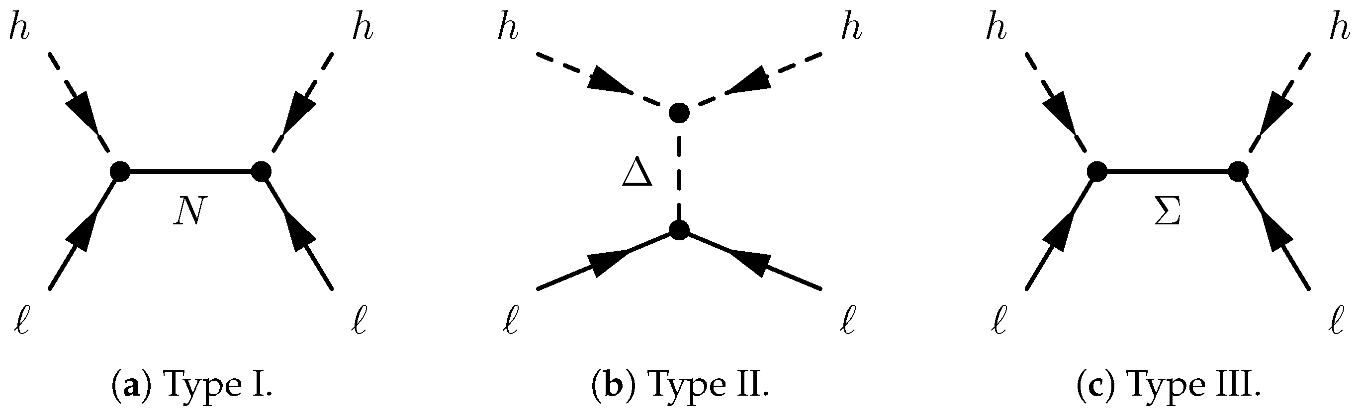
3.1. Mass Generation for Neutrinos as Majorana Fermions

A particularly compelling scheme to address the smallness of neutrino masses is the seesaw mechanism [33,34,35,36,37,38,39,40,41]. In its simplest form [33,34,35,36,38,39], right-handed neutrinos are introduced. The existence of such right-handed neutrinos is motivated by the scheme of GUT: in particular, the SO(10) model [42], in which right-handed neutrinos are unavoidably predicted. Integrating them out leads to the Weinberg operator
L κ = 1 4 κ g f C , g ¯ h f h + h . c . ,
where f denotes the left-handed lepton doublets of the SM, h is the Higgs doublet, and g and f are the family indices. Equation (1) is the unique dimension-five operator consistent with the symmetries of the SM. In the canonical seesaw mechanism, κ g f scales like the inverse of the masses of the right-handed neutrinos M, and the smallness of the active neutrino mass eigenvalues m ν is explained via the famous seesaw formula
m ν ( m ν Dirac ) 2 M .
Here, the Dirac neutrino mass, m ν Dirac , is given by the product of the Dirac neutrino Yukawa matrix Y ν and the Higgs vacuum expectation value (VEV). Of course, (2) is to be understood as the shorthand for a matrix equation. There are variations of the canonical seesaw, known as type II [37,38,39] and type III [40,41], in which heavy SU ( 2 ) L triplets are exchanged. The different variants are depicted in Figure 2.
For collider experimental tests of some of the low-scale variants of the seesaw mechanisms, see [43].

3.2. Radiative Neutrino Masses

The underlying idea of the so-called radiative neutrino mass models (see e.g., [44] for a review) is that neutrino masses, which are absent at the tree level, may become induced via loops, thus addressing the smallness of neutrino masses. This option was pioneered by Zee [45].
Here, we will use the so-called scotogenic model [46] to review some of the relevant facts. A nice overview for this model can be found in [44] (Section 5.3). This model contains the SM fermions, three singlet fermions N f , as well as an extra doublet η that has the same SM quantum numbers as the SM Higgs doublet h but is distinguished by an extra Z 2 symmetry. In more detail, both N f as well as η are odd under this Z 2 , whereas the usual SM fields are even. This Z 2 forbids Yukawa couplings between , h, and N but allows for couplings between , η , and N. However, there are interactions between h and η via a scalar potential, and these interactions give rise to a loop diagram (cf. Figure 3) that induces an effective Weinberg operator and thus neutrino masses.
Note that this diagram requires a coupling R e ( h η ) 2 . As explained in [44] (Section 5.3), this term breaks the “generalized lepton number” symmetry that the Lagrange density would otherwise have, which forbids (Majorana) neutrino masses. A point that will be relevant for our later discussion in Section 4 and Section 5 is that this model, in the presence of the above-mentioned quartic coupling, does not have a symmetry that forbids the Weinberg operator. So one could a priori just add it to the model. However, all the terms required for the model to work are renormalizable. Therefore, even if a tree-level Weinberg operator exists, for a large enough cut-off scale Λ , its contribution to the light neutrino masses can be suppressed against the loop term. In this sense, the neutrino masses are generated by loops even though other contributions are not completely forbidden.
Thus, this renormalizable model can provide us with robust relations between the model parameters and neutrino data. Later, in Section 4 and Section 5, we will see that extra contributions cannot always be sufficiently suppressed in constructions that rely on higher-dimensional operators without explicit UV completion.

3.3. Dirac Neutrino Masses

The charged SM fermions get their masses from Dirac mass terms, which combine two different Weyl spinors. This option is also valid for neutrinos, for which these mass terms then originate from the Yukawa terms
L ν Dirac = Y ν g f f ¯ h N g + h . c . ,
where N g denotes the right-handed neutrinos. While small fermion masses are said to be technically natural, the required Yukawa couplings | Y ν g f | 10 12 beg for an explanation. Rather compelling mechanisms have been put forward in the past. Many of these mechanisms rely on ingredients in new physics scenarios that aim at solving the gauge hierarchy problem. These include supersymmetry [47], radiative mechanisms [48,49], warped extra dimensions [50,51], and more recently, the clockwork mechanism [52,53,54]. Dirac neutrino masses may also just arise at higher orders [55]. While these possibilities can be argued to deserve more attention, in the following, we restrict our focus on seesaw scenarios for Majorana neutrinos.

3.4. Neutrino Masses in Explicit String Models

A long-standing question is what string theory says about neutrino masses [56]. The answer is model-dependent. It has been proposed that the smallness of neutrino masses may be due to their origin from instantons [57]. However, an explicit SM-like model featuring this scenario has yet to be found. On the other hand, the heterotic string provides us with an abundance of explicit SM-like models with seesaw-suppressed neutrino masses [58]. Importantly, in string models, the spectrum is fixed, and one can simply count the number of right-handed neutrinos. It turns out that, unlike in bottom-up models, their number is of the order N ν = O ( 10 , , 100 ) . This means that the Weinberg operator (1) receives contributions from many neutrinos.
Universe 09 00512 i001
This effectively lowers the seesaw scale, i.e., even if the individual right-handed neutrino mass eigenvalues are of the order of the GUT scale O ( 10 16 ) GeV , realistic active neutrino masses can emerge. It has further been found in [59] that the contribution of many neutrinos can mimic the anarchy scenario [60,61,62], in which large mixing angles are statistically favored.
On the other hand, in string models, one cannot only count the right-handed neutrinos, one can, at least in principle, compute the couplings. These couplings are often constrained by “traditional” flavor symmetries, which we will study in Section 4. Moreover, additional constraints arise from modular symmetries, which are intrinsic to string theory; we will discuss these symmetries, their origin, and their role in phenomenology in Section 5. That is, in what follows, we will concentrate on an alternate, i.e., non-anarchic, approach to understand the origin of flavor. Specifically, we will discuss how the observed large mixing angles may arise from the dynamics of certain underlying fundamental symmetries.

4. Traditional Flavor Symmetries
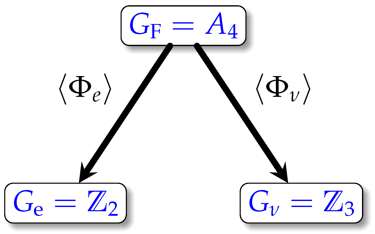
A curious feature of the SM is the repetition of families, i.e., the fact that SM matter appears in three copies of particles transforming in identical representations under the SM gauge group:
G SM = SU ( 3 ) C × SU ( 2 ) L × U ( 1 ) Y .
This repetition may be the consequence of a so-called horizontal or flavor symmetry. Continuous flavor symmetries often suffer from anomalies and/or unrealistic Goldstone modes, so a lot of attention has been given to non-Abelian finite groups [5] (see, e.g., [63] for a review). These symmetries are less challenged by Goldstone modes1. Imposing such flavor symmetries can help to reduce the number of free parameters and lead to nontrivial predictions. It is not the purpose of this paper to survey all flavor models (for reviews and references, see, e.g., [63,72]). Rather, in what follows, we will illustrate some of the main prospects and challenges using a concrete example.

4.1. Example: A 4

4.1.1. Explicit Model

One particularly popular example of a finite flavor symmetry for the lepton sector of the SM is the alternating group of order 4: A 4 [73,74,75,76]. An explicit A 4 -based example assumes low-energy supersymmetry (SUSY), and the relevant superpotential terms are given by [76]
W ν = λ 1 Λ Λ ν L H u L H u 3 Φ ν 1 + λ 2 Λ Λ ν L H u L H u 1 ξ ,
W e = h e Λ Φ e L 1 H d e R + h μ Λ Φ e L 1 H d μ R + h τ Λ Φ e L 1 H d τ R .
Here, L, e R , μ R , τ R , H u , and H d , respectively, denote the lepton doublets, charged leptons, u-type Higgs, and d-type Higgs of the (minimal) supersymmetric SM. The lepton doublets, L = ( L e , L μ , L τ ) T , are assumed to transform as an A 4 3 -plet. The right-handed charged lepton fields, μ R and τ R , transform in the one-dimensional representations 1 and 1 of A 4 , respectively. The Higgs doublets and e R are trivial A 4 singlets. The fields Φ ν , Φ e , and ξ are so-called flavons and are assumed to transform as 3 , 3 , and 1 , respectively. Λ denotes the cut-off, and Λ ν is the seesaw scale. The subscripts 1 , 3 , and so on denote contractions to a 1 -plet, 3 -plet, etc.
The flavons are assumed to attain certain VEVss:
Φ ν = v , v , v ,
Φ e = v , 0 , 0 ,
ξ = w ,
where v, v , and w are some dimensionful parameters that are to be explained through a suitable mechanism that aligns the VEVs, a point that we will expand on below in Section 4.1.3. To first approximations, these VEVss break A 4 down to G e = Z 2 in the charged lepton sector and to G ν = Z 3 in the neutrino sector, cf. Figure 4. These approximate symmetries fix the neutrino superpotential to be given by [76]:
W ν = L e H u , L μ H u , L τ H u a + 2 d d d d 2 d a d d a d 2 d L e H u L μ H u L τ H u
up to corrections that we will discuss below in Section 4.1.2. The entries of the mass matrix in Equation (8) depend, at leading order, only on the parameters a = 2 λ 1 λ 2 w Λ 1 Λ ν and d = λ 1 3 v Λ 1 Λ ν . At the same time, the charged lepton superpotential leads to diagonal Yukawa couplings:
W e = L e , L μ , L τ y e 0 0 0 y μ 0 0 0 y τ e R μ R τ R H d ,
where y e , μ , τ = h e , μ , τ v Λ . As a result, the mixing is of the so-called tribimaximal form [77], i.e., the PMNS [8] matrix is given by
U PMNS TBM = 2 3 1 3 0 1 6 1 3 1 2 1 6 1 3 1 2 .
This corresponds to the leptonic mixing angles
θ 12 35 , θ 13 = 0 and θ 23 = 45 .
Even though these very angles are no longer consistent with the data, they could be regarded as a step towards a realistic mixing model.
The main point to make in the context of this model is that non-Abelian flavor symmetries may provide us with predictions of the mixing angles that are, to some approximation, independent of the continuous parameters of the model.
However, given the sheer number of models that appear to describe observation one may wonder how robust the predictions really are. In other words, if many different symmetries are consistent with the data we have, to which extent do these symmetries really predict the observed pattern of masses and mixings? In what follows, we shall review some of the limitations shared by many models based on finite groups.

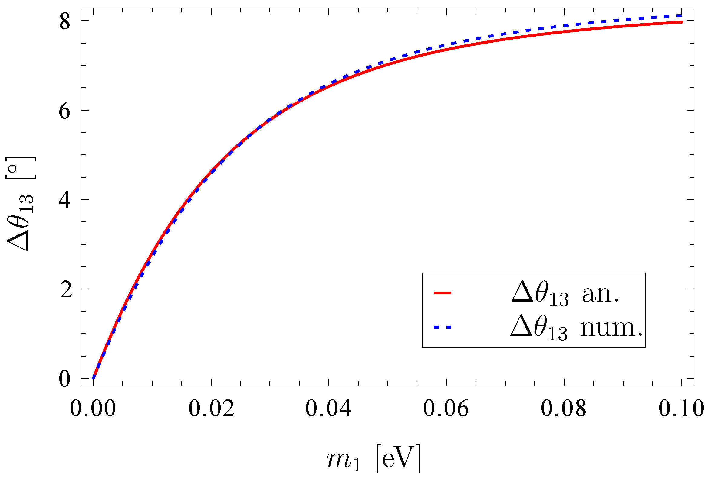
4.1.2. Corrections and Limitations

As we have seen in Section 2, specifically Table 1 and Figure 1, our experimental community has determined the neutrino parameters with an impressive accuracy, which will even be dramatically improved further in the near future. It is, therefore, natural to ask what the error bars in the predictions from the models are. It turns out that often the error bars are not specified. However, in the (bottom-up) models, there are often substantial uncertainties. It is rather easy to see why this is. These models are usually effective field theorys (EFTs), i.e., defined by the symmetries and particle content, and endowed with a cut-off, Λ , as is the case in our example in (6). The symmetries get spontaneously broken by some flavon VEVs, and one finds rather modest hierarchies in explicit flavor models: often, the ratio of a typical flavon VEV over the cut-off scale is of the order of the Cabbibo angle, ε : = Φ / Λ 0.2 . The best one can do in an EFT framework is to perform an expansion in ε , and these qualitative arguments suggest that there are correction on the order of 20 % compared to predictions.
However, qualitative arguments do not always lead to the correct conclusions, so one may wonder if these corrections arise, and if so, how. It turns out that in supersymmetric theories, higher-order terms in the superpotential can often be forbidden by some carefully crafted R and non-R symmetries. Likewise, quantum corrections from the renormalization group equations (RGEs) have been worked out analytically (cf. e.g., [78]), and while there is still room for relevant corrections in the minimal supersymmetric standard model (MSSM) with large Higgs VEV ratio tan β , typically their impact is limited (see, e.g., [79] for a comprehensive analysis).
On the other hand, it is known that in many models, corrections to the kinetic terms have a significant impact on the predicted values of observables [80,81]. The main problem is that in a pure bottom-up EFT approach, one cannot forbid higher-order terms in the Kähler potential that couple the flavons to the matter fields nor the analogous terms in non-supersymmetric models. Those terms can induce the O ( ε ) corrections that one expects to find from the above qualitative argument. Specifically, for the A 4 model, it has been shown that the Kähler corrections are often far larger than the experimental uncertainties in the mixing parameters [82,83]. In particular, there are additional free, i.e., not predicted by the model, parameters that allow one to adjust the predictions at will. We show an example in Figure 5. As one can see, even under rather conservative assumptions, the corrections to the prediction exceed the experimental error bars by far. In particular, including these terms, as one should, can render the A 4 model from completely ruled out to perfectly consistent. Likewise, these terms, which cannot be controlled in the bottom-up approach, can also change consistent models to ruled-out constructions.

4.1.3. VEV Alignment

Another subtle aspect of the model is the VEV alignment. That is, rather than postulating the VEVs (7), there should be a dynamical reason why these values are assumed. It turns out that one can sometimes construct models in which the desired VEVss emerge by minimizing a flavon potential, and this is more straightforward if those VEVss respect certain residual symmetries, as is the case in the A 4 model [76,84,85,86,87]. However, in practice, this often comes at the expense of introducing ad hoc symmetries and extra fields. Some of these extra fields are frequently referred to as “driving fields”, but they really should be regarded as Lagrange multipliers used to impose additional conditions on the VEVs that sometimes appear to be ad hoc, i.e., having no other purpose than to create the desired VEVs. Furthermore, these driving fields can introduce more parameters to the theory that, in turn, reduce the predictive power of the theory. Adding these driving fields introduces new “free” parameters, which may or may not have a direct impact on the relevant predictions. Note also that the corrections described in Section 4.1.2 can also affect the VEV alignment. It has also been shown in [88] that one may also achieve VEV alignment by imposing boundary conditions of scalar fields in extra dimensions.

4.2. C P Violation from Finite Groups

Let us briefly comment on another curious property of finite groups. It turns out that finite groups may, unlike continuous (or Lie) groups, clash with C P [89,90]. This means that some groups do not comply with a physical C P transformation. Notice that there is sometimes some confusion in the literature. C P transformations can be generalized [91,92]. However, some of the transformations that have been dubbed “generalized C P transformations” do not warrant C P conservation and may more appropriately be referred to as C P -like transformations [90,93]. On the other hand, some groups do not admit proper C P transformations [90] and thus clash with C P . It turns out that these C P -violating groups are not at all exotic: for instance, all odd-order finite groups are of this type. Yet there are also even-order groups of this type, such as Δ ( 54 ) , which is the traditional flavor symmetry [94] of some of the earliest string models [95] and for which C P violation is tied to the presence of winding modes [96], i.e., the very modes that are instrumental for the UV completion of the model. This leaves us with the remarkable picture that flavor symmetries can very well be the reason why C P is violated, which also fits nicely with the observation that all of the C P violations found so far in Nature reside in the flavor sector. One may thus hope to obtain new solutions to the strong C P problem [97]. However, so far, a concrete realization of this idea has been hindered by the limitations discussed in Section 4.1.2. Yet the new ideas that we shall review in Section 5 may provide us with the mileage required to construct a concrete model.

4.3. Origin of Flavor Symmetries

While one can obviously impose flavor symmetries in a bottom-up approach, one may wonder if they have a top-down motivation. The answer to this question is affirmative. It has been shown that such symmetries can emerge in various string models, such as heterotic orbifolds [94], intersecting D-branes [98], and F-theory [99].

4.4. Where to Go from Here?

As we have seen, non-Abelian discrete flavor symmetries may motivate the repetition of families and provide us with an interpretation of the observed mixing parameters. However, as discussed above, there are also limitations. One major obstacle is VEV alignment. As we shall see in the following section, modular flavor symmetries evade some of the complications and have an arguably more direct connection to UV completions of the SM.

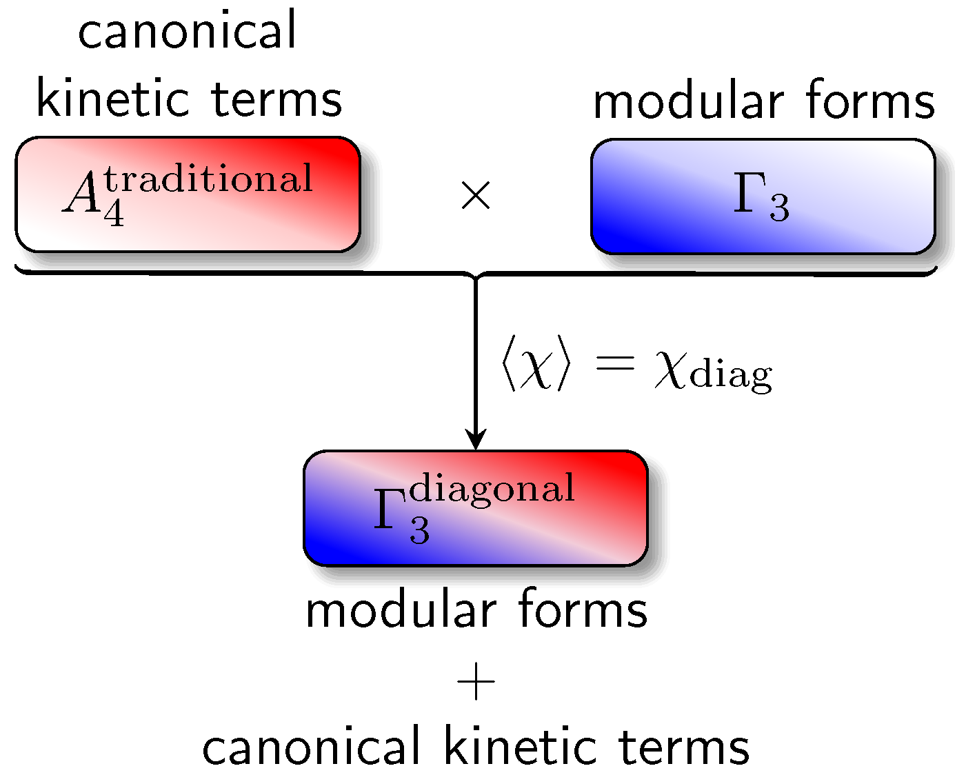
5. Modular Flavor Symmetries

A few years ago, Feruglio put forward a rather minimal and very successful model [4] based on a modular version of the A 4 discussed in Section 4.1. This model has received significant attention (cf. e.g., [79,100,101,102,103,104,105,106,107,108,109,110,111,112,113,114]) because it largely avoids the complications of VEV alignment and is, at some level, able to make a large number of nontrivial predictions. This type of model uses the so-called modular flavor symmetries, which we shall review in what follows.

5.1. Modular Transformations

Let us first recall what modular transformations are. They can be thought of as transformations that map a given torus on an equivalent torus. A 2-torus T 2 emerges as the quotient C / Z 2 . That is, two points in the complex plane are identified if they differ by a lattice vector n 1 e 1 + n 2 e 2 , with the e α C denoting linearly independent basis vectors and the n α Z for α { 1 , 2 } . However, one can change the basis vectors without changing the lattice. The allowed transformations are (cf., e.g., [115])
e 2 e 1 γ e 2 e 1 = a b c d e 2 e 1 = : γ e 2 e 1 .
Here, γ is a SL ( 2 , Z ) matrix, i.e.,
a , b , c , d Z and a d b c = 1 .
As is well known, the shape of a given torus is parametrized by the so-called half-period ratio τ : = e 2 / e 1 . Without loss of generality, one can demand that Im τ > 0 . Furthermore, under (12), τ undergoes the modular transformations
τ γ a τ + b c τ + d .

5.2. Modular Forms

Holomorphic functions of τ complying with (14) are known to be rather constrained. We are specifically interested in so-called modular forms, which transform under γ (cf. Equation (14)) as
f ( τ ) γ f γ ( τ ) = f a τ + b c τ + d = ( c τ + d ) k f ( τ ) .
Here, k is the so-called modular weight, which is sometimes taken to be an integer, but in top-down models, it often happens to be a rational number2. In order to understand how this story is related to finite groups, perhaps the most direct way is to consider the theory of vector-valued modular forms [116]. The latter transform under (14) as
Y ( τ ) γ Y γ ( τ ) = Y a τ + b c τ + d = ( c τ + d ) k ρ ( γ ) Y ( τ ) .
Here, Y ( τ ) = Y 1 ( τ ) , , Y d ( τ ) is a d -plet, and ρ ( γ ) is a representation matrix of a finite modular group that arises from the quotient of SL ( 2 , Z ) (or one of its multiple covers) divided by any of its normal subgroups.

5.3. Modular Flavor Symmetries in the Bottom-Up Approach

In order to see how the modular flavor symmetries allow us to avoid the subtleties of VEV alignment to a large degree, let us review some aspects of the Feruglio model [4]. Rather than a “traditional” A 4 as in Section 4.1, this model is based on a “modular” A 4 . This allows us to replace the Φ ν flavon by a triplet of known functions of τ :
Φ ν = ( Φ ν ) 1 ( Φ ν ) 2 ( Φ ν ) 3 Y 1 ( τ ) Y 2 ( τ ) Y 3 ( τ ) .
That is, the crucial feature pointed out in [4] is that the three complex components of the flavon Φ ν can be replaced by three functions Y i ( τ ) , which turn out to be modular forms building a triplet and transforming according to Equation (16), where ρ ( γ ) is the triplet representation of the finite modular symmetry A 4 Γ 3 . Importantly, these functions Y i ( τ ) can be explicitly constructed. Consequently, rather than aligning multiple VEVss comprising six real degrees of freedom, one now faces the much more manageable challenge of fixing τ , which has two real degrees of freedom. As has been well known for quite some time, for largish Im τ , these couplings are exponentially suppressed [117,118,119], which is why they appear at first sight more suitable to accommodate the Yukawa couplings of the quarks and charged leptons. However, Feruglio’s fit [4] wants τ to be close to the so-called self-dual point τ = i . Fixing τ is part of what is called moduli stabilization in string phenomenology: see e.g., [120,121] for early references on this topic. Remarkably, in these examples, τ gets fixed at or close to the self-dual point, i.e., where neutrino data want it to be. See also [122] for a discussion of moduli fixing and [123,124,125] for an analysis of hierarchies around τ = i in the context of bottom-up modular flavor symmetries. In this modular model, there is no need for the ξ flavon, which is instrumental in the model discussed in Section 4.1.1 based on a traditional A 4 symmetry. Assuming diagonal charged lepton Yukawa couplings, this model then derives nine predictions from three input parameters:
seesaw scale Λ ν R e τ Im τ 3 neutrino masses m i 3 mixing angles θ i j 2 Majorana phases φ i 1 C P phase δ C P
This system is overconstrained, as we already know five observables: the two mass-squared differences and three mixing angles. It turns out that this model can nonetheless fit observation surprisingly well. Furthermore, when introducing an extra parameter, called φ 3 , which changes the charged lepton Yukawa matrix to a non-diagonal one, it is possible to obtain fit with Δ χ 2 = 0.4 for inverted ordering and Δ χ 2 = 9.9 for normal ordering (see Tables 4 and 5 of [79], respectively). Here, Δ χ 2 is obtained by comparing the model predictions to the current best-fit values of the mixing angles, charged lepton Yukawa couplings, and neutrino mass differences. Ref. [79] also finds that the corrections from SUSY breaking and RGE corrections are relatively small in their model. This model then makes testable predictions on the C P phases as well as the neutrino mass scale. This is a remarkable result.
It turns out that, similarly to what we already discussed in Section 4.1.2, there are extra terms in this model that are not fixed by the symmetries and that thus introduce additional free parameters [126]. In some ways, this problem is even worse than in the “traditional” case discussed in Section 4.1.2 since modular flavor symmetries are nonlinearly realized and thus provide us with less expansion control.
One can nonetheless show that by borrowing inputs from the “eclectic” scheme that we will discuss in Section 5.5, one can limit the impact of these extra terms to be smaller than the current experimental uncertainties of the observables [127]. In this variation of the Feruglio model [4], a non-modular finite symmetry is added, and the full flavor symmetry is a product of a modular and a traditional symmetry. This product is then broken to a diagonal subgroup (cf. Figure 6) that coincides with the modular A 4 of the Feruglio model [4]. There are still corrections of the order χ / Λ , where χ denotes the flavon accomplishing the diagonal breaking, but this ratio can be as small as the τ Yukawa coupling, which is of the order 10 2 unless tan β is large. Therefore, the uncertainties of the predictions can be made to be comparable to the experimental error bars. While this proof-of-principle example has been carefully crafted to obtain sufficient control over the kinetic terms, the fact that it utilizes ingredients first discussed in the top-down approach may be taken as an indication that a combination of both approaches will ultimately provide us with constructions that are simultaneously elegant, predictive, and realistic.

5.4. Metaplectic Flavor Symmetries

As we have argued in the introduction, the modular flavor symmetries are of particular interest as they hint at top-down physics. A bit more practically, one may want to have an interpretation, say, of the modular weight k in Equations (15) and (16) as well as of the origin of the flavor symmetries. Magnetized tori [128], which are dual to certain D-brane models [129], turn out to be an appropriate playground to answer some of these questions [115,130,131,132,133,134,135,136,137,138,139]. In particular, the modular weights k reflect the localization properties of matter fields in the extra dimensions. This is because the Kähler metric, which depends on τ (as well as other moduli) determines the normalization of the matter fields. Half-integer modular weights then imply that the fields are something in between a bulk field and a brane field. This is reflected by the profiles of the relevant zero modes [128]. We depict the projection of some sample wavefunctions in Figure 7. This picture also offers an intuitive understanding of the well-known exponential suppression of the couplings in the large Im τ limit [117,118,119].
Since modular weights are half-integers, the flavor symmetry is metaplectic rather than modular [137]. These metaplectic flavor symmetries have been discussed in the bottom-up approach [111,113], and the expressions for the Yukawa couplings coincide with those obtained from magnetized tori [137]. That is, Yukawa couplings can be computed in two ways, either in a bottom-up approach by postulating metaplectic flavor symmetries and determining the corresponding modular forms, or in a top-down way by computing the overlaps of wavefunctions on magnetized tori, and the results agree. Although the successful models obtained in the bottom-up approach [111,113] can give predictions within the experimental 1 σ range (see, e.g., Section 4.2 of [111]), these have not yet been derived from the top-down approach. This is because one cannot dial the data like modular weights and representations at will. Yet one may take the phenomenologically successful constructions as a guide to choose geometrical data of the top-down models to come closer to the real world. In this sense, current and ongoing neutrino experiment data may provide us with crucial insights into a possible UV completion of the SM.

5.5. Eclectic Flavor Symmetries

Modular symmetries and modular forms appear quite naturally in top-down scenarios based on a class of string compactifications known as heterotic orbifolds [140,141]. In these models, beyond the 3 + 1 dimensions of our spacetime, the six extra dimensions of a string theory assume the form of complex tori divided by discrete symmetries (see, e.g., [142,143,144] for an introduction to these constructions). This procedure yields a UV complete 3 + 1 -dimensional effective field theory endowed with various continuous and discrete global and gauge symmetries, which are fully determined by the shape of the compact dimensions. Furthermore, the matter spectrum together with its transformation properties under the available symmetries is also fixed by the compactification. In this kind of model, it has been shown that the exact matter spectrum of the SM can be achieved, including quarks and leptons and their mixings [145,146,147,148].
Among the symmetries of these string models, one identifies their discrete flavor symmetries (which technically correspond to the outer automorphisms of the Narain space group associated with the orbifold). The origin and properties of these flavor symmetries have been explored in a series of papers [149,150,151,152,153]. The resulting symmetries lead to the so-called “eclectic” picture, which unifies the traditional flavor symmetries of Section 4 with the modular groups as in Section 5.3. Roughly speaking, the eclectic flavor symmetry is given by
G eclectic = G traditional G modular ,
where “∪” is to be understood as the multiplicative closure. The eclectic symmetries include
  • Traditional flavor symmetries;
  • Modular flavor symmetries;
  • R symmetries (including non-Abelian discrete R symmetries);
  • C P symmetries and C P -like transformations (see Section 4.2 for the distinction).
Interestingly, both R and C P (and C P -like) symmetries are linked to modular transformations, arising from SL ( 2 , Z ) or even Sp ( 2 g , Z ) [153]. (The latter has also been explored in the bottom-up approach [112].) Further, all charges of matter fields, including their modular weights k Q and representations ρ ( γ ) , are fully fixed by the string construction. Whereas the modular weights of matter are fractional in general, it turns out that the couplings among them are governed by integer positive modular weights and are thus modular forms.
This eclectic picture provides a nontrivial mixture of symmetries, which constrains not only the superpotential but also the Kähler potential; i.e., models with eclectic flavor symmetries are more restricted than bottom-up constructions. In fact, these constraints solve the challenges to predictability that bottom-up models endowed with flavor modular symmetries face [126]. This advantage is partly due to the large number of elements of eclectic flavor symmetries (e.g., the eclectic flavor group of a T 2 / Z 2 heterotic orbifold sector has 4608 elements [153]), but it actually follows from the natural appearance of a traditional flavor subgroup within eclectic symmetries. This feature has been exploited, e.g., in the bottom-up quasi-eclectic scenario [127] discussed in Section 5.3.
Reproducing data requires the breakdown of the eclectic flavor symmetry. This is done in two steps: (1) τ is stabilized at a point in modular space, breaking the modular subgroup, and (2) one or more flavons develop VEVs, breaking the remaining traditional flavor symmetry. This leads to a rich variety of flavor symmetry patterns [154], which can in some cases match the mass and mixing textures of quarks and charged leptons observed in nature and yield predictions for the neutrino sector [155], where all corrections are under control. Even though the flavon VEVs can, in principle, be fixed by demanding that supersymmetry is preserved at low energies in these string models, it is fair to say that finding a principle that dynamically fixes both the modulus and flavon VEVs at the right values for phenomenology is still an open question. Moreover, not all possible models based on eclectic flavor symmetries from strings have been phenomenologically investigated. In anticipation of the upcoming neutrino data, it is important to pursue this task now or in the near future.
One can generalize this top-down framework to arrive at bottom-up models endowed with eclectic flavor symmetries. To achieve this goal, one must stress two important features of these symmetries in string constructions. First, it turns out that G modular is always a subgroup of the outer automorphisms of G traditional . Secondly, for a subgroup G of G traditional , Equation (18) takes the form
G eclectic = G G modular , G G traditional ,
which means in particular that G modular and G do not commute. It has been found that these observations hold also in models based on magnetized tori [134]. Using these observations and the definitions of finite modular groups, a large class of bottom-up eclectic flavor symmetries has been constructed [156]. A relevant pending question is what kind of neutrino phenomenology can be obtained from these symmetries. Further, it is clear now that more general eclectic flavor symmetries can be constructed, especially including vector-valued modular forms [116], which might open new avenues for relating neutrino data to possible UV completions of the SM.

5.6. Nonsupersymmetric Modular Flavor Symmetries

In our discussion so far, we always assumed low-energy SUSY, though we are far from certain that it is realized in Nature. It has been argued in [128,137] that low-energy SUSY may, in principle, not be required for the Yukawa couplings to be of the metaplectic form. Further, large classes of explicit string models similar to those presented in Section 5.5 with the exact spectrum of the SM and no SUSY have been built [157,158,159,160]. However, much more effort has to be devoted to better understand their details, including the stability of these models [159,161], the versions of discrete (traditional and modular) flavor symmetries that they exhibit, and, hence, the phenomenology they yield.

6. Summary and Outlook

We have argued that, given the expected wealth of neutrino data, i.e., experimental knowledge of the flavor sector of the SM, it is now the time to sharpen our theoretical understanding of the matter. While measurements become more precise, a fully convincing interpretation of the data has remained elusive so far. The so-called modular flavor symmetries have a clear top-down motivation and, at the same time, arguably provide us with some of the most compelling models of flavor. We have outlined how a successful unification of bottom-up and top-down ideas and techniques may guide us towards a new era of precision flavor model building for which future experimental results can give us crucial insights in the UV completion of the SM.

Author Contributions

Writing—original draft, Y.A., M.-C.C., M.C., V.K.-P., Y.L., A.M., S.R.-S., M.R. and S.S.; Writing—review & editing, Y.A., M.-C.C., M.C., V.K.-P., Y.L., A.M., S.R.-S., M.R. and S.S. All authors have read and agreed to the published version of the manuscript.

Funding

The work of Y.A. is supported by Kuwait University. The work of M.C. is supported by the US Department of Energy under grant No. DE-SC0015640. The work of M.-C.C., V.K.-P., A.M., M.R., and S.S. is supported by the National Science Foundation under grant No. PHY-1915005. This work is also supported by UC-MEXUS-CONACyT grant No. CN-20-38. This work was performed in part at the Aspen Center for Physics, which is supported by National Science Foundation grant PHY-1607611.

Data Availability Statement

Data are contained within the article.

Acknowledgments

We would like to thank Yuri Shirman for discussions and Shirley Li for correspondence.

Conflicts of Interest

The authors declare no conflict of interest.

Abbreviations

CnBCosmic Neutrino Background
EFTeffective field theory
GUTGrand Unified Theory
IOinverted ordering
LHCLarge Hadron Collider
MFVMinimal Flavor Violation
MSSMminimal supersymmetric standard model
NOnormal ordering
NSInon-standard interactions
QFTquantum field theory
RGErenormalization group equation
SBsymmetry based
SMStandard Model of Particle Physics
SUSYsupersymmetry
TBtorus based
UVultraviolet
VEVvacuum expectation value

Notes

1
The anomalies of finite groups can readily be determined [64,65,66,67,68,69], yet their implications have not been worked in great detail so far in the context of (bottom-up) model building. Discrete matching [70] of these anomalies as well as outer automorphism anomalies [71] may provide us with crucial insights on how bottom-up and top-down models are related.
2
For noninteger k, we are technically no longer dealing with modular transformations, a point that we will get back to in Section 5.4.

References

  1. Ferrara, S.; Lüst, D.; Shapere, A.D.; Theisen, S. Modular Invariance in Supersymmetric Field Theories. Phys. Lett. B 1989, 225, 363. [Google Scholar] [CrossRef]
  2. Chun, E.J.; Mas, J.; Lauer, J.; Nilles, H.P. Duality and Landau-ginzburg Models. Phys. Lett. B 1989, 233, 141–146. [Google Scholar] [CrossRef]
  3. Quevedo, F. Lectures on superstring phenomenology. AIP Conf. Proc. 1996, 359, 202–242. [Google Scholar] [CrossRef]
  4. Feruglio, F. Are neutrino masses modular forms? In From My Vast Repertoire …: Guido Altarelli’s Legacy; Levy, A., Forte, S., Ridolfi, G., Eds.; World Scientific Publishing: Singapore, 2019; pp. 227–266. [Google Scholar] [CrossRef]
  5. Kaplan, D.B.; Schmaltz, M. Flavor unification and discrete nonAbelian symmetries. Phys. Rev. D 1994, 49, 3741–3750. [Google Scholar] [CrossRef] [PubMed]
  6. Pontecorvo, B. Inverse beta processes and nonconservation of lepton charge. Zh. Eksp. Teor. Fiz. 1957, 34, 247. [Google Scholar]
  7. Gribov, V.N.; Pontecorvo, B. Neutrino astronomy and lepton charge. Phys. Lett. B 1969, 28, 493. [Google Scholar] [CrossRef]
  8. Maki, Z.; Nakagawa, M.; Sakata, S. Remarks on the unified model of elementary particles. Prog. Theor. Phys. 1962, 28, 870–880. [Google Scholar] [CrossRef]
  9. Fukuda, Y. et al. [Super-Kamiokande Collaboration] Evidence for oscillation of atmospheric neutrinos. Phys. Rev. Lett. 1998, 81, 1562–1567. [Google Scholar] [CrossRef]
  10. Ahmad, Q.R. et al. [SNO Collaboration] Measurement of the rate of νe+dp+p+e interactions produced by 8B solar neutrinos at the Sudbury Neutrino Observatory. Phys. Rev. Lett. 2001, 87, 071301. [Google Scholar] [CrossRef]
  11. Esteban, I.; González-García, M.C.; Maltoni, M.; Schwetz, T.; Zhou, A. The fate of hints: Updated global analysis of three-flavor neutrino oscillations. J. High Energy Phys. 2020, 2020, 178. [Google Scholar] [CrossRef]
  12. Esteban, I.; González-García, M.C.; Maltoni, M.; Schwetz, T.; Zhou, A. Available online: http://www.nu-fit.org/ (accessed on 1 April 2022).
  13. Abe, K. et al. [The T2K Collaboration] Constraint on the matter–antimatter symmetry-violating phase in neutrino oscillations. Nature 2020, 580, 339–344, Erratum in Nature 2020, 583, E16. [Google Scholar] [CrossRef] [PubMed]
  14. Esteban, I.; González-García, M.C.; Hernández-Cabezudo, A.; Maltoni, M.; Schwetz, T. Global analysis of three-flavour neutrino oscillations: Synergies and tensions in the determination of θ23, δCP, and the mass ordering. J. High Energy Phys. 2019, 2019, 106. [Google Scholar] [CrossRef]
  15. Chatterjee, S.S.; Palazzo, A. Resolving the NOvA and T2K tension in the presence of Neutrino Non-Standard Interactions. PoS 2022, 402, 059. [Google Scholar] [CrossRef]
  16. Acero, M.A. et al. [The NOvA Collaboration] An Improved Measurement of Neutrino Oscillation Parameters by the NOvA Experiment. arXiv 2021, arXiv:hep-ex/2108.08219. [Google Scholar]
  17. Abe, K. et al. [Hyper-Kamiokande Proto-Collaboration] Hyper-Kamiokande Design Report. arXiv 2018, arXiv:physics.ins-det/1805.04163. [Google Scholar]
  18. Acciarri, R. et al. [DUNE Collaboration] Long-Baseline Neutrino Facility (LBNF) and Deep Underground Neutrino Experiment (DUNE): Conceptual Design Report, Volume 1: The LBNF and DUNE Projects. arXiv 2016, arXiv:physics.ins-det/1601.05471. [Google Scholar]
  19. Smirnov, M.V.; Hu, Z.J.; Li, S.J.; Ling, J.J. The possibility of leptonic CP-violation measurement with JUNO. Nucl. Phys. B 2018, 931, 437–445. [Google Scholar] [CrossRef]
  20. Song, N.; Li, S.W.; Argüelles, C.A.; Bustamante, M.; Vincent, A.C. The Future of High-Energy Astrophysical Neutrino Flavor Measurements. J. Cosmol. Astropart. Phys. 2021, 04, 054. [Google Scholar] [CrossRef]
  21. Denton, P.B.; Parke, S.J.; Zhang, X. Neutrino oscillations in matter via eigenvalues. Phys. Rev. D 2020, 101, 093001. [Google Scholar] [CrossRef]
  22. Qian, X.; Vogel, P. Neutrino Mass Hierarchy. Prog. Part. Nucl. Phys. 2015, 83, 1–30. [Google Scholar] [CrossRef]
  23. Lee, C.M.; Selby, J.H. Higher-Order Interference in Extensions of Quantum Theory. Found. Phys. 2016, 47, 89–112. [Google Scholar] [CrossRef]
  24. Xu, B. Neutrino Decoherence in Simple Open Quantum Systems. arXiv 2020, arXiv:hep-ph/2009.13471. [Google Scholar]
  25. Agostini, M.; Benato, G.; Detwiler, J.A.; Menéndez, J.; Vissani, F. Toward the discovery of matter creation with neutrinoless double-beta decay. arXiv 2022, arXiv:hep-ex/2202.01787. [Google Scholar]
  26. Cirigliano, V.; Davoudi, Z.; Dekens, W.; de Vries, J.; Engel, J.; Feng, X.; Gehrlein, J.; Graesser, M.L.; Gráf, L.; Hergert, H.; et al. Neutrinoless Double-Beta Decay: A Roadmap for Matching Theory to Experiment. arXiv 2022, arXiv:hep-ph/2203.12169. [Google Scholar]
  27. Gastaldo, L.; Blaum, K.; Chrysalidis, K.; Goodacre, T.D.; Domula, A.; Door, M.; Dorrer, H.; Düllmann, C.E.; Eberhardt, K.; Eliseev, S.; et al. The electron capture in163Ho experiment–ECHo. Eur. Phys. J. Spec. Top. 2017, 226, 1623–1694. [Google Scholar] [CrossRef]
  28. Aker, M.; Balzer, M.; Batzler, D.; Beglarian, A.; Behrens, J.; Berlev, A.; Besserer, U.; Biassoni, M.; Bieringer, B.; Block, F.; et al. KATRIN: Status and prospects for the neutrino mass and beyond. J. Phys. G 2022, 49, 100501. [Google Scholar] [CrossRef]
  29. Betti, M.G.; Biasotti, M.; Boscá, A.; Calle, F.; Canci, N.; Cavoto, G.; Chang, C.; Cocco, A.G.; Colijn, A.P.; Conrad, J.; et al. Neutrino physics with the PTOLEMY project: Active neutrino properties and the light sterile case. J. Cosmol. Astropart. Phys. 2019, 7, 047. [Google Scholar] [CrossRef]
  30. Ashtari Esfahani, A.; Asner, D.M.; Böser, S.; Cervantes, R.; Claessens, C.; de Viveiros, L.; Doe, P.J.; Doeleman, S.; Fernandes, J.L.; Fertl, M.; et al. Determining the neutrino mass with cyclotron radiation emission spectroscopy—Project 8. J. Phys. G 2017, 44, 054004. [Google Scholar] [CrossRef]
  31. Danilov, M. Review of sterile neutrino searches at very short-baseline reactor experiments. arXiv 2022, arXiv:hep-ex/2203.03042. [Google Scholar] [CrossRef]
  32. Coloma, P.; Esteban, I.; González-García, M.C.; Larizgoitia, L.; Monrabal, F.; Palomares-Ruiz, S. Bounds on new physics with data of the Dresden-II reactor experiment and COHERENT. arXiv 2022, arXiv:hep-ph/2202.10829. [Google Scholar] [CrossRef]
  33. Minkowski, P. μ at a Rate of One Out of 109 Muon Decays? Phys. Lett. B 1977, 67, 421–428. [Google Scholar] [CrossRef]
  34. Yanagida, T. Horizontal gauge symmetry and masses of neutrinos. Conf. Proc. C 1979, 7902131, 95–99. [Google Scholar]
  35. Glashow, S.L. The Future of Elementary Particle Physics. NATO Sci. Ser. B 1980, 61, 687. [Google Scholar] [CrossRef]
  36. Gell-Mann, M.; Ramond, P.; Slansky, R. Complex Spinors and Unified Theories. Conf. Proc. C 1979, 790927, 315–321. [Google Scholar]
  37. Magg, M.; Wetterich, C. Neutrino Mass Problem and Gauge Hierarchy. Phys. Lett. B 1980, 94, 61–64. [Google Scholar] [CrossRef]
  38. Lazarides, G.; Shafi, Q. Neutrino Masses in SU(5). Phys. Lett. B 1981, 99, 113–116. [Google Scholar] [CrossRef]
  39. Mohapatra, R.N.; Senjanovic, G. Neutrino Mass and Spontaneous Parity Violation. Phys. Rev. Lett. 1980, 44, 912. [Google Scholar] [CrossRef]
  40. Mohapatra, R.N.; Senjanovic, G. Neutrino Masses and Mixings in Gauge Models with Spontaneous Parity Violation. Phys. Rev. D 1981, 23, 165. [Google Scholar] [CrossRef]
  41. Foot, R.; Lew, H.; He, X.G.; Joshi, G.C. Seesaw Neutrino Masses Induced by a Triplet of Leptons. Z. Phys. C 1989, 44, 441. [Google Scholar] [CrossRef]
  42. Fritzsch, H.; Minkowski, P. Unified Interactions of Leptons and Hadrons. Ann. Phys. 1975, 93, 193–266. [Google Scholar] [CrossRef]
  43. Fuks, B.; Neundorf, J.; Peters, K.; Ruiz, R.; Saimpert, M. Probing the Weinberg operator at colliders. Phys. Rev. D 2021, 103, 115014. [Google Scholar] [CrossRef]
  44. Cai, Y.; Herrero-García, J.; Schmidt, M.A.; Vicente, A.; Volkas, R.R. From the trees to the forest: A review of radiative neutrino mass models. Front. in Phys. 2017, 5, 63. [Google Scholar] [CrossRef]
  45. Zee, A. A Theory of Lepton Number Violation, Neutrino Majorana Mass, and Oscillation. Phys. Lett. B 1980, 93, 389, Erratum in Phys. Lett. B 1980, 95, 461. [Google Scholar] [CrossRef]
  46. Ma, E. Verifiable radiative seesaw mechanism of neutrino mass and dark matter. Phys. Rev. D 2006, 73, 077301. [Google Scholar] [CrossRef]
  47. Arkani-Hamed, N.; Hall, L.J.; Murayama, H.; Tucker-Smith, D.; Weiner, N. Small neutrino masses from supersymmetry breaking. Phys. Rev. D 2001, 64, 115011. [Google Scholar] [CrossRef]
  48. Babu, K.S.; He, X.G. Dirac Neutrino Masses as Two Loop Radiative Corrections. Mod. Phys. Lett. A 1989, 4, 61. [Google Scholar] [CrossRef]
  49. Farzan, Y.; Pascoli, S.; Schmidt, M.A. Recipes and Ingredients for Neutrino Mass at Loop Level. J. High Energy Phys. 2013, 2013, 107. [Google Scholar] [CrossRef]
  50. Grossman, Y.; Neubert, M. Neutrino masses and mixings in nonfactorizable geometry. Phys. Lett. B 2000, 474, 361–371. [Google Scholar] [CrossRef]
  51. Huber, S.J.; Shafi, Q. Fermion masses, mixings and proton decay in a Randall-Sundrum model. Phys. Lett. B 2001, 498, 256–262. [Google Scholar] [CrossRef]
  52. Park, S.C.; Shin, C.S. Clockwork seesaw mechanisms. Phys. Lett. B 2018, 776, 222–226. [Google Scholar] [CrossRef]
  53. Hong, S.; Kurup, G.; Perelstein, M. Clockwork Neutrinos. J. High Energy Phys. 2019, 2019, 73. [Google Scholar] [CrossRef]
  54. Babu, K.S.; Saad, S. Flavor Hierarchies from Clockwork in SO(10) GUT. Phys. Rev. D 2021, 103, 015009. [Google Scholar] [CrossRef]
  55. Babu, K.S.; Leung, C.N. Classification of effective neutrino mass operators. Nucl. Phys. B 2001, 619, 667–689. [Google Scholar] [CrossRef]
  56. Giedt, J.; Kane, G.L.; Langacker, P.; Nelson, B.D. Massive neutrinos and (heterotic) string theory. Phys. Rev. D 2005, 71, 115013. [Google Scholar] [CrossRef]
  57. Blumenhagen, R.; Cvetič, M.; Weigand, T. Spacetime instanton corrections in 4D string vacua: The Seesaw mechanism for D-Brane models. Nucl. Phys. B 2007, 771, 113–142. [Google Scholar] [CrossRef]
  58. Buchmüller, W.; Hamaguchi, K.; Lebedev, O.; Ramos-Sánchez, S.; Ratz, M. Seesaw neutrinos from the heterotic string. Phys. Rev. Lett. 2007, 99, 021601. [Google Scholar] [CrossRef]
  59. Feldstein, B.; Klemm, W. Large Mixing Angles From Many Right-Handed Neutrinos. Phys. Rev. D 2012, 85, 053007. [Google Scholar] [CrossRef]
  60. Hall, L.J.; Murayama, H.; Weiner, N. Neutrino mass anarchy. Phys. Rev. Lett. 2000, 84, 2572–2575. [Google Scholar] [CrossRef]
  61. De Gouvea, A.; Murayama, H. Statistical test of anarchy. Phys. Lett. B 2003, 573, 94–100. [Google Scholar] [CrossRef]
  62. De Gouvea, A.; Murayama, H. Neutrino Mixing Anarchy: Alive and Kicking. Phys. Lett. B 2015, 747, 479–483. [Google Scholar] [CrossRef]
  63. Ishimori, H.; Kobayashi, T.; Ohki, H.; Shimizu, Y.; Okada, H.; Tanimoto, M. Non-Abelian Discrete Symmetries in Particle Physics. Prog. Theor. Phys. Suppl. 2010, 183, 1–163. [Google Scholar] [CrossRef]
  64. Araki, T. Anomaly of Discrete Symmetries and Gauge Coupling Unification. Prog. Theor. Phys. 2007, 117, 1119–1138. [Google Scholar] [CrossRef]
  65. Araki, T.; Kobayashi, T.; Kubo, J.; Ramos-Sánchez, S.; Ratz, M.; Vaudrevange, P.K.S. (Non-)Abelian discrete anomalies. Nucl. Phys. B 2008, 805, 124–147. [Google Scholar] [CrossRef]
  66. Chen, M.C.; Fallbacher, M.; Ratz, M.; Trautner, A.; Vaudrevange, P.K.S. Anomaly-safe discrete groups. Phys. Lett. B 2015, 747, 22–26. [Google Scholar] [CrossRef]
  67. Talbert, J. Pocket Formulae for Non-Abelian Discrete Anomaly Freedom. Phys. Lett. B 2018, 786, 426–431. [Google Scholar] [CrossRef]
  68. Kobayashi, T.; Uchida, H. Anomaly of non-Abelian discrete symmetries. Phys. Rev. D 2022, 105, 036018. [Google Scholar] [CrossRef]
  69. Gripaios, B. Gauge anomalies of finite groups. arXiv 2022, arXiv:hep-th/2201.11801. [Google Scholar] [CrossRef]
  70. Csáki, C.; Murayama, H. Discrete anomaly matching. Nucl. Phys. B 1998, 515, 114–162. [Google Scholar] [CrossRef]
  71. Henning, B.; Lu, X.; Melia, T.; Murayama, H. Outer automorphism anomalies. J. High Energy Phys. 2022, 2022, 94. [Google Scholar] [CrossRef]
  72. Feruglio, F.; Romanino, A. Lepton flavor symmetries. Rev. Mod. Phys. 2021, 93, 15007. [Google Scholar] [CrossRef]
  73. Ma, E.; Rajasekaran, G. Softly broken A(4) symmetry for nearly degenerate neutrino masses. Phys. Rev. D 2001, 64, 113012. [Google Scholar] [CrossRef]
  74. Babu, K.S.; Ma, E.; Valle, J.W.F. Underlying A(4) symmetry for the neutrino mass matrix and the quark mixing matrix. Phys. Lett. B 2003, 552, 207–213. [Google Scholar] [CrossRef]
  75. Hirsch, M.; Romao, J.C.; Skadhauge, S.; Valle, J.W.F.; Villanova del Moral, A. Phenomenological tests of supersymmetric A(4) family symmetry model of neutrino mass. Phys. Rev. D 2004, 69, 093006. [Google Scholar] [CrossRef]
  76. Altarelli, G.; Feruglio, F. Tri-bimaximal neutrino mixing from discrete symmetry in extra dimensions. Nucl. Phys. B 2005, 720, 64–88. [Google Scholar] [CrossRef]
  77. Harrison, P.F.; Perkins, D.H.; Scott, W.G. Tri-bimaximal mixing and the neutrino oscillation data. Phys. Lett. B 2002, 530, 167. [Google Scholar] [CrossRef]
  78. Antusch, S.; Kersten, J.; Lindner, M.; Ratz, M.; Schmidt, M.A. Running neutrino mass parameters in see-saw scenarios. J. High Energy Phys. 2005, 2005, 24. [Google Scholar] [CrossRef]
  79. Criado, J.C.; Feruglio, F. Modular Invariance Faces Precision Neutrino Data. SciPost Phys. 2018, 5, 42. [Google Scholar] [CrossRef]
  80. Leurer, M.; Nir, Y.; Seiberg, N. Mass matrix models: The Sequel. Nucl. Phys. B 1994, 420, 468–504. [Google Scholar] [CrossRef]
  81. Dudas, E.; Pokorski, S.; Savoy, C.A. Yukawa matrices from a spontaneously broken Abelian symmetry. Phys. Lett. B 1995, 356, 45–55. [Google Scholar] [CrossRef]
  82. Chen, M.C.; Fallbacher, M.; Ratz, M.; Staudt, C. On predictions from spontaneously broken flavor symmetries. Phys. Lett. B 2012, 718, 516–521. [Google Scholar] [CrossRef]
  83. Chen, M.C.; Fallbacher, M.; Omura, Y.; Ratz, M.; Staudt, C. Predictivity of models with spontaneously broken non-Abelian discrete flavor symmetries. Nucl. Phys. B 2013, 873, 343–371. [Google Scholar] [CrossRef]
  84. Bazzocchi, F.; Kaneko, S.; Morisi, S. A SUSY A(4) model for fermion masses and mixings. J. High Energy Phys. 2008, 2008, 63. [Google Scholar] [CrossRef]
  85. Feruglio, F.; Hagedorn, C.; Merlo, L. Vacuum Alignment in SUSY A4 Models. J. High Energy Phys. 2010, 2010, 84. [Google Scholar] [CrossRef]
  86. King, S.F.; Luhn, C. Trimaximal neutrino mixing from vacuum alignment in A4 and S4 models. J. High Energy Phys. 2011, 2011, 42. [Google Scholar] [CrossRef]
  87. Holthausen, M.; Schmidt, M.A. Natural Vacuum Alignment from Group Theory: The Minimal Case. J. High Energy Phys. 2012, 2012, 126. [Google Scholar] [CrossRef]
  88. Kobayashi, T.; Omura, Y.; Yoshioka, K. Flavor Symmetry Breaking and Vacuum Alignment on Orbifolds. Phys. Rev. D 2008, 78, 115006. [Google Scholar] [CrossRef]
  89. Chen, M.C.; Mahanthappa, K.T. Group Theoretical Origin of CP Violation. Phys. Lett. B 2009, 681, 444–447. [Google Scholar] [CrossRef]
  90. Chen, M.C.; Fallbacher, M.; Mahanthappa, K.T.; Ratz, M.; Trautner, A. CP Violation from Finite Groups. Nucl. Phys. B 2014, 883, 267–305. [Google Scholar] [CrossRef]
  91. Feruglio, F.; Hagedorn, C.; Ziegler, R. Lepton Mixing Parameters from Discrete and CP Symmetries. J. High Energy Phys. 2013, 2013, 27. [Google Scholar] [CrossRef]
  92. Holthausen, M.; Lindner, M.; Schmidt, M.A. CP and Discrete Flavour Symmetries. J. High Energy Phys. 2013, 2013, 122. [Google Scholar] [CrossRef]
  93. Trautner, A. CP and Other Symmetries of Symmetries. Ph.D. Thesis, Technical University of Munich, München, Germany, 2016. Available online: https://arxiv.org/abs/1608.05240 (accessed on 1 April 2022).
  94. Kobayashi, T.; Nilles, H.P.; Plöger, F.; Raby, S.; Ratz, M. Stringy origin of non-Abelian discrete flavor symmetries. Nucl. Phys. B 2007, 768, 135–156. [Google Scholar] [CrossRef]
  95. Ibáñez, L.E.; Kim, J.E.; Nilles, H.P.; Quevedo, F. Orbifold Compactifications with Three Families of SU(3) × SU(2) × U(1)n. Phys. Lett. B 1987, 191, 282–286. [Google Scholar] [CrossRef]
  96. Nilles, H.P.; Ratz, M.; Trautner, A.; Vaudrevange, P.K.S. CP violation from string theory. Phys. Lett. B 2018, 786, 283–287. [Google Scholar] [CrossRef]
  97. Ratz, M.; Trautner, A. CP violation with an unbroken CP transformation. J. High Energy Phys. 2017, 2017, 103. [Google Scholar] [CrossRef]
  98. Abe, H.; Choi, K.S.; Kobayashi, T.; Ohki, H. Non-Abelian Discrete Flavor Symmetries from Magnetized/Intersecting Brane Models. Nucl. Phys. B 2009, 820, 317–333. [Google Scholar] [CrossRef]
  99. Cvetič, M.; Heckman, J.J.; Lin, L. Towards Exotic Matter and Discrete Non-Abelian Symmetries in F-theory. J. High Energy Phys. 2018, 2018, 1. [Google Scholar] [CrossRef]
  100. Kobayashi, T.; Tanaka, K.; Tatsuishi, T.H. Neutrino mixing from finite modular groups. Phys. Rev. D 2018, 98, 016004. [Google Scholar] [CrossRef]
  101. De Anda, F.J.; King, S.F.; Perdomo, E. SU(5) grand unified theory with A4 modular symmetry. Phys. Rev. D 2020, 101, 015028. [Google Scholar] [CrossRef]
  102. Okada, H.; Tanimoto, M. CP violation of quarks in A4 modular invariance. Phys. Lett. B 2019, 791, 54–61. [Google Scholar] [CrossRef]
  103. Ding, G.J.; King, S.F.; Liu, X.G. Neutrino mass and mixing with A5 modular symmetry. Phys. Rev. D 2019, 100, 115005. [Google Scholar] [CrossRef]
  104. Novichkov, P.; Penedo, J.; Petcov, S.; Titov, A. Generalised CP Symmetry in Modular-Invariant Models of Flavour. J. High Energy Phys. 2019, 2019, 165. [Google Scholar] [CrossRef]
  105. Liu, X.G.; Ding, G.J. Neutrino Masses and Mixing from Double Covering of Finite Modular Groups. J. High Energy Phys. 2019, 2019, 134. [Google Scholar] [CrossRef]
  106. Kobayashi, T.; Shimizu, Y.; Takagi, K.; Tanimoto, M.; Tatsuishi, T.H. A4 lepton flavor model and modulus stabilization from S4 modular symmetry. Phys. Rev. D 2019, 100, 115045, Erratum in Phys. Rev. D 2020, 101, 039904. [Google Scholar] [CrossRef]
  107. Asaka, T.; Heo, Y.; Tatsuishi, T.H.; Yoshida, T. Modular A4 invariance and leptogenesis. J. High Energy Phys. 2020, 2020, 144. [Google Scholar] [CrossRef]
  108. Ding, G.J.; King, S.F.; Liu, X.G.; Lu, J.N. Modular S4 and A4 symmetries and their fixed points: New predictive examples of lepton mixing. J. High Energy Phys. 2019, 2019, 30. [Google Scholar] [CrossRef]
  109. Kobayashi, T.; Shimizu, Y.; Takagi, K.; Tanimoto, M.; Tatsuishi, T.H.; Uchida, H. CP violation in modular invariant flavor models. Phys. Rev. D 2020, 101, 055046. [Google Scholar] [CrossRef]
  110. Ding, G.J.; Feruglio, F. Testing Moduli and Flavon Dynamics with Neutrino Oscillations. J. High Energy Phys. 2020, 2020, 134. [Google Scholar] [CrossRef]
  111. Liu, X.G.; Yao, C.Y.; Qu, B.Y.; Ding, G.J. Half-integral weight modular forms and application to neutrino mass models. Phys. Rev. D 2020, 102, 115035. [Google Scholar] [CrossRef]
  112. Ding, G.J.; Feruglio, F.; Liu, X.G. Automorphic Forms and Fermion Masses. J. High Energy Phys. 2021, 2021, 37. [Google Scholar] [CrossRef]
  113. Yao, C.Y.; Liu, X.G.; Ding, G.J. Fermion masses and mixing from the double cover and metaplectic cover of the A5 modular group. Phys. Rev. D 2021, 103, 095013. [Google Scholar] [CrossRef]
  114. Novichkov, P. Aspects of the Modular Symmetry Approach to Lepton Flavour. Ph.D. Thesis, Scuola Internazionale Superiore di Studi Avanzati (SISSA), Trieste, Italy, 2021. [Google Scholar]
  115. Kikuchi, S.; Kobayashi, T.; Uchida, H. Modular flavor symmetries of three-generation modes on magnetized toroidal orbifolds. Phys. Rev. D 2021, 104, 065008. [Google Scholar] [CrossRef]
  116. Liu, X.G.; Ding, G.J. Modular flavor symmetry and vector-valued modular forms. J. High Energy Phys. 2022, 2022, 123. [Google Scholar] [CrossRef]
  117. Dine, M.; Seiberg, N.; Wen, X.G.; Witten, E. Nonperturbative Effects on the String World Sheet. Nucl. Phys. B 1986, 278, 769–789. [Google Scholar] [CrossRef]
  118. Dine, M.; Seiberg, N.; Wen, X.G.; Witten, E. Nonperturbative Effects on the String World Sheet. 2. Nucl. Phys. B 1987, 289, 319–363. [Google Scholar] [CrossRef]
  119. Cvetič, M. Suppression of Nonrenormalizable Terms in the Effective Superpotential for (Blownup) Orbifold Compactification. Phys. Rev. Lett. 1987, 59, 1795. [Google Scholar] [CrossRef] [PubMed]
  120. Font, A.; Ibáñez, L.E.; Lüst, D.; Quevedo, F. Supersymmetry Breaking From Duality Invariant Gaugino Condensation. Phys. Lett. B 1990, 245, 401–408. [Google Scholar] [CrossRef]
  121. Nilles, H.P.; Olechowski, M. Gaugino Condensation and Duality Invariance. Phys. Lett. B 1990, 248, 268–272. [Google Scholar] [CrossRef]
  122. Novichkov, P.P.; Penedo, J.T.; Petcov, S.T. Modular Flavour Symmetries and Modulus Stabilisation. arXiv 2022, arXiv:hep-ph/2201.02020. [Google Scholar] [CrossRef]
  123. Okada, H.; Tanimoto, M. Modular invariant flavor model of A4 and hierarchical structures at nearby fixed points. Phys. Rev. D 2021, 103, 015005. [Google Scholar] [CrossRef]
  124. Feruglio, F.; Gherardi, V.; Romanino, A.; Titov, A. Modular invariant dynamics and fermion mass hierarchies around τ=i. J. High Energy Phys. 2021, 2021, 242. [Google Scholar] [CrossRef]
  125. Novichkov, P.P.; Penedo, J.T.; Petcov, S.T. Fermion mass hierarchies, large lepton mixing and residual modular symmetries. J. High Energy Phys. 2021, 2021, 206. [Google Scholar] [CrossRef]
  126. Chen, M.C.; Ramos-Sánchez, S.; Ratz, M. A note on the predictions of models with modular flavor symmetries. Phys. Lett. B 2020, 801, 135153. [Google Scholar] [CrossRef]
  127. Chen, M.C.; Knapp-Pérez, V.; Ramos-Hamud, M.; Ramos-Sánchez, S.; Ratz, M.; Shukla, S. Quasi-eclectic modular flavor symmetries. Phys. Lett. B 2022, 824, 136843. [Google Scholar] [CrossRef]
  128. Cremades, D.; Ibáñez, L.E.; Marchesano, F. Computing Yukawa couplings from magnetized extra dimensions. J. High Energy Phys. 2004, 2004, 79. [Google Scholar] [CrossRef]
  129. Cremades, D.; Ibáñez, L.E.; Marchesano, F. Yukawa couplings in intersecting D-brane models. J. High Energy Phys. 2003, 2003, 38. [Google Scholar] [CrossRef]
  130. Kobayashi, T.; Nagamoto, S.; Uemura, S. Modular symmetry in magnetized/intersecting D-brane models. Prog. Theor. Exp. Phys. 2017, 2017, 023B02. [Google Scholar] [CrossRef]
  131. Kobayashi, T.; Nagamoto, S.; Takada, S.; Tamba, S.; Tatsuishi, T.H. Modular symmetry and non-Abelian discrete flavor symmetries in string compactification. Phys. Rev. D 2018, 97, 116002. [Google Scholar] [CrossRef]
  132. Kobayashi, T.; Tamba, S. Modular forms of finite modular subgroups from magnetized D-brane models. Phys. Rev. D 2019, 99, 046001. [Google Scholar] [CrossRef]
  133. Kariyazono, Y.; Kobayashi, T.; Takada, S.; Tamba, S.; Uchida, H. Modular symmetry anomaly in magnetic flux compactification. Phys. Rev. D 2019, 100, 045014. [Google Scholar] [CrossRef]
  134. Ohki, H.; Uemura, S.; Watanabe, R. Modular flavor symmetry on a magnetized torus. Phys. Rev. D 2020, 102, 085008. [Google Scholar] [CrossRef]
  135. Kikuchi, S.; Kobayashi, T.; Takada, S.; Tatsuishi, T.H.; Uchida, H. Revisiting modular symmetry in magnetized torus and orbifold compactifications. Phys. Rev. D 2020, 102, 105010. [Google Scholar] [CrossRef]
  136. Kikuchi, S.; Kobayashi, T.; Otsuka, H.; Takada, S.; Uchida, H. Modular symmetry by orbifolding magnetized T2×T2: Realization of double cover of ΓN. J. High Energy Phys. 2020, 2020, 101. [Google Scholar] [CrossRef]
  137. Almumin, Y.; Chen, M.C.; Knapp-Pérez, V.; Ramos-Sánchez, S.; Ratz, M.; Shukla, S. Metaplectic Flavor Symmetries from Magnetized Tori. J. High Energy Phys. 2021, 2021, 78. [Google Scholar] [CrossRef]
  138. Tatsuta, Y. Modular symmetry and zeros in magnetic compactifications. J. High Energy Phys. 2021, 2021, 54. [Google Scholar] [CrossRef]
  139. Kikuchi, S.; Kobayashi, T.; Nasu, K.; Uchida, H.; Uemura, S. Modular symmetry anomaly and non-perturbative neutrino mass terms in magnetized orbifold models. arXiv 2022, arXiv:hep-th/2202.05425. [Google Scholar]
  140. Lauer, J.; Mas, J.; Nilles, H.P. Duality and the Role of Nonperturbative Effects on the World Sheet. Phys. Lett. B 1989, 226, 251–256. [Google Scholar] [CrossRef]
  141. Lauer, J.; Mas, J.; Nilles, H.P. Twisted sector representations of discrete background symmetries for two-dimensional orbifolds. Nucl. Phys. B 1991, 351, 353–424. [Google Scholar] [CrossRef]
  142. Bailin, D.; Love, A. Orbifold compactifications of string theory. Phys. Rept. 1999, 315, 285–408. [Google Scholar] [CrossRef]
  143. Ramos-Sánchez, S. Towards Low Energy Physics from the Heterotic String. Fortsch. Phys. 2009, 10, 907–1036. [Google Scholar] [CrossRef]
  144. Vaudrevange, P.K.S. Grand Unification in the Heterotic Brane World. Ph.D. Thesis, University of Bonn, Bonn, Germany, 2008. [Google Scholar]
  145. Nilles, H.P.; Ramos-Sánchez, S.; Ratz, M.; Vaudrevange, P.K.S. From strings to the MSSM. Eur. Phys. J. C 2009, 59, 249–267. [Google Scholar] [CrossRef]
  146. Kappl, R.; Petersen, B.; Raby, S.; Ratz, M.; Schieren, R.; Vaudrevange, P.K.S. String-Derived MSSM Vacua with Residual R Symmetries. Nucl. Phys. B 2011, 847, 325–349. [Google Scholar] [CrossRef]
  147. Nilles, H.P.; Vaudrevange, P.K.S. Geography of Fields in Extra Dimensions: String Theory Lessons for Particle Physics. Mod. Phys. Lett. A 2015, 30, 1530008. [Google Scholar] [CrossRef]
  148. Parr, E.; Vaudrevange, P.K.S. Contrast data mining for the MSSM from strings. Nucl. Phys. B 2020, 952, 114922. [Google Scholar] [CrossRef]
  149. Nilles, H.P.; Ramos-Sánchez, S.; Vaudrevange, P.K.S. Eclectic flavor scheme from ten-dimensional string theory—II detailed technical analysis. Nucl. Phys. B 2021, 966, 115367. [Google Scholar] [CrossRef]
  150. Baur, A.; Kade, M.; Nilles, H.P.; Ramos-Sánchez, S.; Vaudrevange, P.K.S. The eclectic flavor symmetry of the Z2 orbifold. J. High Energy Phys. 2021, 2021, 18. [Google Scholar] [CrossRef]
  151. Nilles, H.P.; Ramos-Sánchez, S.; Vaudrevange, P.K.S. Eclectic flavor scheme from ten-dimensional string theory—I. Basic results. Phys. Lett. B 2020, 808, 135615. [Google Scholar] [CrossRef]
  152. Nilles, H.P.; Ramos-Sánchez, S.; Vaudrevange, P.K.S. Lessons from eclectic flavor symmetries. Nucl. Phys. B 2020, 957, 115098. [Google Scholar] [CrossRef]
  153. Baur, A.; Kade, M.; Nilles, H.P.; Ramos-Sánchez, S.; Vaudrevange, P.K.S. Completing the eclectic flavor scheme of the Z2 orbifold. J. High Energy Phys. 2021, 2021, 110. [Google Scholar] [CrossRef]
  154. Baur, A.; Nilles, H.P.; Ramos-Sánchez, S.; Trautner, A.; Vaudrevange, P.K.S. Top-down anatomy of flavor symmetry breakdown. Phys. Rev. D 2022, 105, 055018. [Google Scholar] [CrossRef]
  155. Baur, A.; Nilles, H.P.; Ramos-Sánchez, S.; Trautner, A.; Vaudrevange, P.K.S. The first string-derived eclectic flavor model with realistic phenomenology. J. High Energy Phys. 2022, 09, 224. [Google Scholar] [CrossRef]
  156. Nilles, H.P.; Ramos-Sánchez, S.; Vaudrevange, P.K. Eclectic Flavor Groups. J. High Energy Phys. 2020, 2020, 45. [Google Scholar] [CrossRef]
  157. Blaszczyk, M.; Groot Nibbelink, S.; Loukas, O.; Ramos-Sánchez, S. Non-supersymmetric heterotic model building. J. High Energy Phys. 2014, 2014, 119. [Google Scholar] [CrossRef]
  158. Ashfaque, J.M.; Athanasopoulos, P.; Faraggi, A.E.; Sonmez, H. Non-Tachyonic Semi-Realistic Non-Supersymmetric Heterotic String Vacua. Eur. Phys. J. C 2016, 76, 208. [Google Scholar] [CrossRef]
  159. Abel, S.; Dienes, K.R.; Mavroudi, E. Towards a nonsupersymmetric string phenomenology. Phys. Rev. D 2015, 91, 126014. [Google Scholar] [CrossRef]
  160. Pérez-Martínez, R.; Ramos-Sánchez, S.; Vaudrevange, P.K.S. Landscape of promising nonsupersymmetric string models. Phys. Rev. D 2021, 104, 046026. [Google Scholar] [CrossRef]
  161. Groot Nibbelink, S.; Loukas, O.; Mütter, A.; Parr, E.; Vaudrevange, P.K.S. Tension Between a Vanishing Cosmological Constant and Non-Supersymmetric Heterotic Orbifolds. Fortsch. Phys. 2020, 68, 2000044. [Google Scholar] [CrossRef]
Figure 1. Current and expected precision of measurements for leptonic parameters in three-neutrino flavor framework [20]. Courtesy of Shirley Li.
Universe 09 00512 g001
Figure 2. Seesaw diagrams. The canonical seesaw mechanism is also referred to as Type I. Here, N is a right-handed neutrino, whereas Δ and Σ are scalar and fermionic SU ( 2 ) L triplets, respectively.
Universe 09 00512 g002
Figure 3. One-loop diagram inducing neutrino masses. Recreated from [44] (Section 5.3).
Universe 09 00512 g003
Figure 4. Approximate partial breaking of A 4 .
Universe 09 00512 g004
Figure 5. Change in θ 13 due to the Kähler correction coming from the term ( L Φ ν ) 3 a ( L Φ ν ) 3 s + h . c . . Here, m 1 is the smallest neutrino mass in NO, the coefficient of this term has been taken to be 1, and the ratio of VEV over the cut-off is 0.2 . The continuous line shows the result when using a linear approximation, while the dashed line shows the result of a numerical computation. See Equation (3.8) and Figure 2 of [82]. Similar plots are obtained for the other mixing angles.
Universe 09 00512 g005
Figure 6. “Quasi-eclectic” symmetries. Taken from [127].
Universe 09 00512 g006
Figure 7. Overlap of two wavefunctions with separation a on a torus. The overlap of a given, say red, curve is not just the overlap with one blue curve but with infinitely many of them due to the periodic nature of the torus. A representative space of the torus lattice is called the fundamental domain. Taken from [137].
Universe 09 00512 g007
Table 1. Current best-fit values of the leptonic mixing parameters. Taken from [11,12].
without SK atmospheric data Normal Ordering (best fit)Inverted Ordering ( Δ χ 2 = 2.6 )
bfp ± 1 σ 3 σ rangebfp ± 1 σ 3 σ range
sin 2 θ 12 0.304 0.012 + 0.013 0.269 0.343 0.304 0.012 + 0.012 0.269 0.343
θ 12 / 33.44 0.74 + 0.77 31.27 35.86 33.45 0.74 + 0.77 31.27 35.87
sin 2 θ 23 0.573 0.023 + 0.018 0.405 0.620 0.578 0.021 + 0.017 0.410 0.623
θ 23 / 49.2 1.3 + 1.0 39.5 52.0 49.5 1.2 + 1.0 39.8 52.1
sin 2 θ 13 0.02220 0.00062 + 0.00068 0.02034 0.02430 0.02238 0.00062 + 0.00064 0.02053 0.02434
θ 13 / 8.57 0.12 + 0.13 8.20 8.97 8.60 0.12 + 0.12 8.24 8.98
δ C P / 194 25 + 52 105 405 287 32 + 27 192 361
Δ m 21 2 10 5 eV 2 7.42 0.20 + 0.21 6.82 8.04 7.42 0.20 + 0.21 6.82 8.04
Δ m 3 2 10 3 eV 2 + 2.515 0.028 + 0.028 + 2.431 + 2.599 2.498 0.029 + 0.028 2.584 2.413
with SK atmospheric data Normal Ordering (best fit)Inverted Ordering ( Δ χ 2 = 7.0 )
bfp ± 1 σ 3 σ rangebfp ± 1 σ 3 σ range
sin 2 θ 12 0.304 0.012 + 0.012 0.269 0.343 0.304 0.012 + 0.013 0.269 0.343
θ 12 / 33.45 0.75 + 0.77 31.27 35.87 33.45 0.75 + 0.78 31.27 35.87
sin 2 θ 23 0.450 0.016 + 0.019 0.408 0.603 0.570 0.022 + 0.016 0.410 0.613
θ 23 / 42.1 0.9 + 1.1 39.7 50.9 49.0 1.3 + 0.9 39.8 51.6
sin 2 θ 13 0.02246 0.00062 + 0.00062 0.02060 0.02435 0.02241 0.00062 + 0.00074 0.02055 0.02457
θ 13 / 8.62 0.12 + 0.12 8.25 8.98 8.61 0.12 + 0.14 8.24 9.02
δ C P / 230 25 + 36 144 350 278 30 + 22 194 345
Δ m 21 2 10 5 eV 2 7.42 0.20 + 0.21 6.82 8.04 7.42 0.20 + 0.21 6.82 8.04
Δ m 3 2 10 3 eV 2 + 2.510 0.027 + 0.027 + 2.430 + 2.593 2.490 0.028 + 0.026 2.574 2.410
Disclaimer/Publisher’s Note: The statements, opinions and data contained in all publications are solely those of the individual author(s) and contributor(s) and not of MDPI and/or the editor(s). MDPI and/or the editor(s) disclaim responsibility for any injury to people or property resulting from any ideas, methods, instructions or products referred to in the content.

