Strong Gravitational Lensing of Gravitational Waves: A Review

Abstract

The first successful detection of gravitational waves (GWs) opened up a new window to study a realm of the most violent phenomena in the universe, such as coalescences of binary black holes (BH–BH), binary neutron stars (NS–NS), and mixed (BH–NS) systems, which are mostly inaccessible in the electromagnetic window. On the other hand, strong gravitational lensing of distant sources, such as galaxies and quasars, by other massive objects lying closer along the line of sight has become a powerful tool in cosmology and astrophysics. With the increasing sensitivity of the new generation of GW detectors, the chances to detect a strongly lensed GW signal are increasing. When GWs are strongly lensed, magnification of the signal intensity is expected, unveiling binary compact objects otherwise too distant to be detected. Such systems are important for their plethora of applications. Lensed GWs can be a test for general relativity, constrain mass distribution in galaxies or galaxy clusters, and provide cosmography information independently of the local cosmic ladders. In this review, we will provide a theoretical background of the gravitational lensing of GWs, including the wave optics regime, which becomes important in this context. Then we will describe the possible cosmological and astrophysical insight hidden in these signals, and present the state-of-the-art searches of lensed GWs in the present and future GW observatories.

1. Introduction

Both gravitational lensing (GL) and gravitational waves (GWs) are fundamental phenomena predicted by Einstein’s Theory of General Relativity (GR) [1]. Even though their existence was indirectly verified in binary pulsars [2,3], gravitational waves have been detected only recently—on 14 of September 2015 by the LIGO and Virgo collaboration [4]. Since then, GWs showed to the broadest community their capacity in unveiling the previously inaccessible sides of the cosmos (refer to [5,6,7] for a review) and testing the validity of GR in strong field regimes [8,9,10,11]. Currently detected GWs were emitted by the population of double compact objects (DCOs), namely, by coalescing binary neutron stars (NS–NS), mixed black hole and neutron star systems (BH–NS), and binary black holes (BH–BH or BBHs) [12]. After the third observing run (O3) of the Advanced LIGO-Virgo and KAGRA [13,14] network, 90 GW events [15,16] have been detected, the majority of which are BBHs. With the event GW170817, the first NS–NS coalescence has been detected [17] accompanied by electromagnetic counterparts, traced from gamma-rays, through optical to radio bands [18] it elevated multimessenger astronomy to a higher level. It is very likely that GW190814 event was caused by a BH–NS system [19]. Thus, the newly emerged GW astronomy, in less than a decade of its existence, confirmed previous theoretical predictions regarding DCOs: their abundance; properties; details of the last stages of their evolution; and, in the case of BBHs, their very existence in nature. In short, the credibility of solid but purely theoretical predictions has been strongly supported. However, there is still no compelling evidence for gravitational lensing in the observed GW signals [20].

Gravitational lensing is the consequence of deflecting the trajectories of light, waves, or particles near concentrated mass distributions due to the resulting curvature of space–time (see [21] for a review). According to GR, freely moving particles or waves travel along the geodesic, which in curved space is no longer a straight line. Of course, the same principle applies to electromagnetic (EM) waves as well as to gravitational waves [22]. To date, however, only gravitational lensing of EM waves has been observed, first as multiple images of a quasar [23], and later as magnified and distorted images of background galaxies or luminous arcs around clusters of galaxies. Now gravitational lensing is a fundamental tool for astrophysics and cosmology; consult [24,25,26] for a description of the different cosmological applications. Depending on the mass of the lens, its distribution, and how close the light from the source passes by the lens, one can observe different phenomena. One of these phenomena is the distortions of shapes, correlated among the sources affected by the same set of lenses, called weak lensing. On the other hand, in strong lensing, a background source appears as multiple images due to the gravitational deflection of photons by a massive foreground galaxy or galaxy cluster. In the case of the largest lenses, such as galaxy clusters, we expect highly magnified images. The photons that were emitted at the same time from the background source arrive in different images with a relative time delay, ranging from minutes to months for galaxies [27,28,29], and up to years for galaxy clusters [30,31,32].

Gravitational lensing of EM waves is usually described in terms of geometrical optics, however, in the case of gravitational waves, this approach is not always valid. For a GW of a wavelength $\lambda$, comparable to the Schwarzschild radius R${}_S$ of the lens, diffraction effects become non-negligible [33,34,35,36,37,38,39,40,41,42,43,44,45,46,47,48]. The wave-like effects (interference, diffraction) should be studied according to the wave optics (WO) description. Generally, diffraction effects are important for lenses smaller than ${10}^8{M}_{\odot }(\lambda /1AU)$. Wave effects in the gravitational lensing of gravitational waves have been investigated by various authors in the past few decades [37,49,50], but recently, the community regained interest in the field due to the possibility of observing it with the new generation of interferometers, which will work at higher wavelengths [38,39,51,52,53,54,55,56,57]. Hence, in Section 2, we introduce the theoretical foundations of GW lensing. As a starting point in Section 2.2, we chose the WO regime, and introduce the geometric optics description in Section 2.2 as a corresponding limit. Then, Section 3 introduces the most often used lens models (point mass and singular isothermal sphere), and reports the quantities theoretically introduced in Section 2 in the context of these models.

With the third-generation network of ground-based interferometers, including two Cosmic Explorers (CE) [58,59] and one Einstein Telescope (ET) [60,61,62], it is expected to have a enormous number of BBH GW detections, e.g., ∼${10}^5$–${10}^6$ events per year [60] coming from sources up to $z=8$ and $z=100$ [63], respectively. In addition to the ground-based interferometers, space-based interferometers will study other, lower-frequency ranges. LISA, the Laser Interferometer Space Antenna [64,65], will be able to detect the signal emitted from supermassive black holes in the ∼${10}^{-4}$–${10}^{-1}$ Hz range. With interferometers covering such a wide range of frequencies, the detection of lensed GWs is a promising tool to enable numerous scientific pursuits [22,55,66,67,68,69,70,71,72]. Section 4 summarizes the predictions of strongly lensed GW rates for the current and future detectors. Then, the next two Section 5 and Section 6 describe prospects regarding the spectrum of scientific issues, which might be addressed with lensed GWs alone and in combination with their EM counterparts, respectively. Finally, Section 7 summarizes our review.

Throughout this review, we adopt the unit system with light velocity $c=1$ in the theoretical part, while in discussions of practical applications, c is reintroduced into the formulae explicitly. We also use bold notation for vectors.

2. Foundations of Strong Lensing of Gravitational Waves

2.1. Wave Optics Approach to Gravitational Lensing

The standard approach to introduce the theory of strong gravitational lensing taken in most of the textbooks starts with the geometrical optics description in terms of light rays undergoing deflection, or in terms of waveforms propagating according to Fermat’s principle [50,73]. This is fully justified in the case of EM signals, where one should worry about wave effects only in exceptional cases [50]. Things are different for GWs. The frequency range currently probed by ground-based detectors comprises 10 Hz $<f<10$ kHz. Future space-borne detectors will probe 0.1 mHz $<f<100$ mHz (LISA) and 1 mHz $<f<100$ Hz (DECIGO). This corresponds to the GW wavelengths of ${10}^4$ m $<\lambda <{10}^7$ m in ground-based and ${10}^6$ m $<\lambda <{10}^{12}$ m in space-borne detectors. Thus, for the deflectors whose Schwarzschild radii are comparable to $\lambda$, the wave optics approach is crucial. Hence, for ground-based detectors, wave optics should be used for the lenses smaller than ${10}^4{M}_{\odot }$, while in the case of space-borne detectors, this upper mass limit reaches ${10}^9{M}_{\odot }$. For this reason, we begin the introduction to gravitational lensing with the wave optics approach, which already has a rich body of work dedicated to it in the literature, e.g., [37,39,49,50,51]. Our exposition will follow the approach of [51].

Let us start by writing the line element of space–time (Minkowski or Friedman–Lemaitre–Robertson–Walker) disturbed by the lens [50]

$$d{s}^2=-(1+2U)d{t}^2+(1-2U)d{\mathit{r}}^2=g_{\mu \nu }d{x}^{\mu }d{x}^{\nu }$$

(1)

where $U\left(\mathit{r}\right)$ denotes the Newtonian gravitational potential of the lens, with the condition $U\ll 1$. Let us further consider a point source emitting spherical, monochromatic GWs of frequency $\omega$ propagating through a lens and finally reaching an observer. The perturbation of the background metric $g_{\mu \nu }$ due to GWs is $h_{\mu \nu }=\varphi e_{\mu \nu }$. Since the polarization tensor $e_{\mu \nu }$ is parallel-transported along the null geodesic, one may neglect its change (being of order $\sim U\left(\mathit{r}\right)<<1$) and study the propagation equation of the scalar wave $\varphi (r,t)=\tilde{\varphi }\left(r\right)e^{-i\omega t}$, which is well represented by the scalar wave equation [49,50]

$${\partial }_{\mu }\left(\sqrt{-g}{g}^{\mu \nu }{\partial }_{\nu }\varphi \right)=0$$

(2)

To the first order in U, Equation (2) can be rewritten as

$$({\nabla }^2+{\omega }^2)\tilde{\varphi }=4{\omega }^{2}U\tilde{\varphi }.$$

(3)

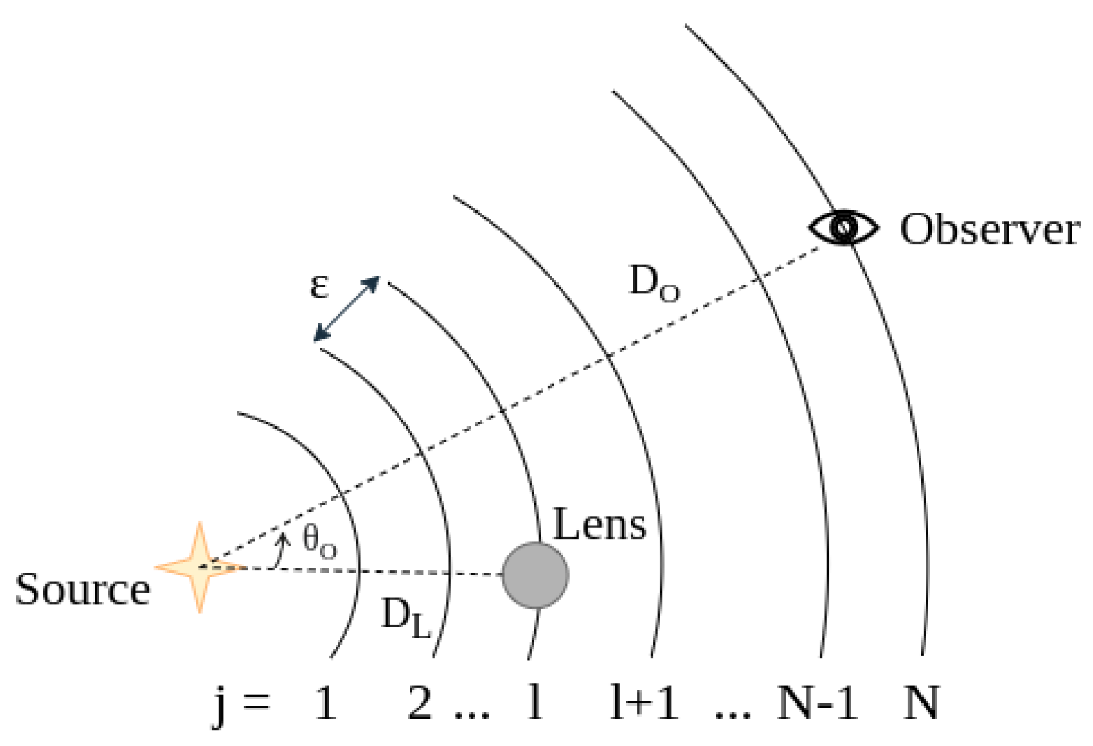
In gravitational lensing, the deflection of a wave by the lens potential is considered to be instantaneous—thin lens approximation. This approximation is justified by the cosmological distances between the lens, source, and observer compared to the size of the region in which the lensing occurs. Under this approximation, the lens mass is projected on a plane, the so-called lens plane. The wave propagates without any interaction, only when ‘hitting’ the lens plane the deflection (or better, the distortion of the wave) occurs. Let us note here that in this section, our presentation differs from the usual style taken in the strong lensing literature, where one anchors the reference frame with the lens, then the deflection and associated ‘new’ position of the source is evident. This is, however, inherently related to the geometric optics limit. Hence, Figure 1 is different from typical strong lensing images.

To describe this system, we consider a set of spherical coordinates $(r,\theta ,\phi )$ with the origin centered on the source and the polar axis pointing towards the lens. We set the observer at ${\mathit{r}}_O=(D_O,{\theta }_O,{\phi }_O)$, far from the source, therefore, ${\theta }_O\ll 1$. In the same way, the waves detected by the observer are confined in the coordinate plane, with $\theta \ll 1$ giving $sin\theta \approx \theta$ and, therefore, the polar vector $\mathsf{\theta }=\theta (cos\phi ,sin\phi )$ behaves as a two-dimensional vector on a flat plane. Consequently, the two-dimensional Laplacian is ${\nabla }_{\theta }^2=\frac{{\partial }^2}{\partial {\theta }^2}+{\theta }^{-1}\frac{\partial }{\partial \theta }+{\theta }^{-2}\frac{{\partial }^2}{\partial {\phi }^2}$.

When a waveform encounters the lens, its path and amplitude undergo some distortions; an undisturbed wave has an amplitude ${\tilde{\varphi }}_0\left(r\right)=A{e}^{i\omega r}/r$, hence, the amplification induced by the lens is defined as

$$F\left(\mathit{r}\right)=\tilde{\varphi }\left(\mathit{r}\right)/{\tilde{\varphi }}_0\left(\mathit{r}\right)$$

(4)

We will refer to this quantity as the amplification factor, as in [51], but in [74], it is also referred to as the transmission function. Rewriting the propagation equations in terms of F, one obtains

$$\frac{{\partial }^{2}F}{\partial r^2}+2i\omega \frac{\partial F}{\partial r}+\frac{1}{r^2}{\nabla }_{\theta }^{2}F=4{\omega }^{2}UF.$$

(5)

By further assuming that $\omega /|\partial lnF/\partial r|\sim$ (scale on which F varies)/ wavelength $\gg 1$, the first term can be neglected. With these approximations, Equation (5) resembles the Schrödinger equation, so one can take advantage of the methods developed in quantum mechanics to study gravitational lensing in the wave optics regime. In particular, the amplification factor can be calculated as a solution of a corresponding path integral based on the classical Lagrangian $L(r,\mathsf{\theta },\dot{\mathsf{\theta }})=\omega \left[\frac{1}{2}{r}^2\left|{\dot{\mathsf{\theta }}}^2\right|-2U(r,\mathsf{\theta })\right],$ where $\dot{\mathsf{\theta }}=d\mathsf{\theta }/dr$. Hence,

$$F\left({\mathit{r}}_{\mathbf{0}}\right)=\int \mathcal{D}\mathsf{\theta }\left(r\right)exp\left\{i{\int }_0^{r_0}drL[r,\mathsf{\theta }\left(r\right),\dot{\mathsf{\theta }}\left(r\right)]\right\}$$

(6)

where the radial function $\mathsf{\theta }\left(r\right)$ represents the path from the source to the observer at ${\mathit{r}}_{\mathit{O}}=(D_O,{\mathsf{\theta }}_{\mathit{O}})$ (see Figure 1), and the integral is over all possible paths. Using the standard approach proposed by Feynman and Hibbs [75], one can consider a grid of concentric spheres having a radius of $r_j=jϵ,j\in \mathbb{N}$, where $ϵ=D_O/N$, ultimately taking a limit of $N\to +\infty$. Therefore, the paths are ${\mathsf{\theta }}_{\mathit{j}}=\mathsf{\theta }\left(r_j\right)$ with $j=1,\cdots ,N$; the lens is placed on the lens plane, i.e., at the l-th sphere, with $D_{LS}=lϵ$ distance from the source. Using the thin lens approximation $U(r,\mathsf{\theta })\to \frac{1}{2}\delta (r-r_L)\widehat{\psi }\left(\mathsf{\theta }\right)$ with $\widehat{\psi }\left(\mathsf{\theta }\right)=2{\int }_0^{r_0}drU(r,\mathsf{\theta })$, one can obtain the following expression for Equation (6):

$$F\left({\mathit{r}}_0\right)=\left[\prod _{j=1}^{N-1}\int \frac{d^2{\mathsf{\theta }}_j}{A_j}\right]exp\left\{i\omega \left[ϵ\sum _{j=1}^{N-1}\frac{r_j{r}_{j+1}}{2}{\left|\frac{{\mathsf{\theta }}_{\mathit{j}}-{\mathsf{\theta }}_{\mathit{j}+\mathbf{1}}}{ϵ}\right|}^2-\widehat{\psi }\left({\mathsf{\theta }}_L\right)\right]\right\}$$

(7)

where $A_j=\frac{2\pi iϵ}{\omega r_j{r}_{j+1}}$ is a normalization factor ensuring that $F=1$ if $\widehat{\psi }=0$. This expression can have a straightforward generalization to the case of multi-lens systems, which is beyond the scope of the present paper.

The first $l-1$ integrals are Gaussian, while the subsequent $j=l+1,\cdots ,N-1$ terms can also be reduced to certain Gaussian integrals (see the Appendix of [51]), and the final result is the so-called Kirchhoff diffraction integral [50]:

$$F\left({\mathit{r}}_0\right)=\frac{\omega }{2\pi i}\frac{D_L{D}_S}{D_{LS}}\int d^2\mathsf{\theta }exp\left\{i\omega \left[\frac{D_L{D}_S}{2D_{LS}}{\left|\mathsf{\theta }-\mathsf{\beta }\right|}^2-\widehat{\psi }\left(\mathsf{\theta }\right)\right]\right\}$$

(8)

for which we have introduced the notations commonly used in the literature regarding gravitational lensing theory. Namely, $\mathsf{\theta }$ is the angular separation between the lens and the image as seen by the observer; $\mathsf{\beta }$ is the angle between the distance from the observer to the source’s true location and to the lens; $D_L$, $D_S$, and $D_{LS}$ are distances to the lens, to the source, and between the lens and the source (see Figure 2).

So far our considerations tacitly assumed Euclidean space, while in most of the real cases of strong lensing, sources and lenses are located at cosmological distances from the observer. Hence, the notion of distances should be made specific. Namely, they have a meaning of the angular–diameter distances $D^A\left(z\right)$, which in the FLRW metric (1) are related by $D^A\left(z\right)=D^C\left(z\right)/(1+z)$ to the comoving distance $D^C\left(z\right)={\int }_0^{z}d{z}^{\prime }/H\left(z^{\prime }\right)$, with z being the redshift and $H\left(z\right)$ the expansion rate. Note that $D^A\left(z_S\right)\ne D^A\left(z_L\right)+D_{LS}^A$ [50], whereas $D^C\left(z_S\right)=D^C\left(z_L\right)+D_{LS}^C$ in the flat FLRW (in non-flat cosmologies this relation should also be modified according to the so-called distance sum rule [76]). From now on, we will explicitly consider cosmological effects and introduce redshifts of the lens $z_L$ and the source $z_S$ appropriately.

The Kirchhoff integral is the most important equation for studying wave effects in gravitational lensing. It expresses the amplification factor F in terms of the frequency of the lensed wave $\omega$ and the relative locations of the elements of the optical system (source, lens, and observer). In Equation (8), there are two distinct contributions in the square brackets. The first one is the geometrical delay, namely, the path length (or travel time [77]) difference between the unlensed straight path from the source to the observer and the lensed path that crosses the lens plane at $\theta$. The second term is the additional contribution introduced by the presence of the lens, i.e., the gravitational time delay caused by the lens’ gravitational potential. Therefore, the terms in square brackets are generally referred to as time delay or Fermat potential [78,79].

Lensing events are expected to be observable when the source, the lens, and the observer are roughly aligned. This be quantified by saying that the source should lie within the (angular) Einstein radius of the lens

$${\theta }_E=\sqrt{4G{M}_L\frac{D_{LS}}{D_L{D}_S}}\equiv \sqrt{2R_S\frac{D_{LS}}{D_L{D}_S}}.$$

(9)

where $R_S$ the Schwarzschild radius of the lens. The physical Einstein radius in the lens plane is $R_E={\theta }_E{D}_L$. The usefulness of the Einstein radius is that it is the robust estimator of the total lens mass. Moreover, it sets the scale of strong lensing phenomenon. Hence, one can obtain a more compact version of (8) by introducing dimensionless parameters

$$\mathit{x}=\frac{\mathsf{\theta }}{{\theta }_E};\mathit{y}=\frac{\mathsf{\beta }}{{\theta }_E};w\equiv \omega (1+z_L)\frac{D_S{D}_L}{D_{LS}}{\theta }_E^2;\psi =\frac{1}{1+z_L}\frac{D_{LS}}{D_S{D}_L}\frac{1}{{\theta }_E^2}\widehat{\psi }$$

(10)

where we have, from left to right, the dimensionless position of the image, the impact parameter, dimensionless frequency, and lens potential.

Lensed waves follow different paths, and, therefore, their times of flight are different. With the quantities introduced in Equation (10), the time delay functional [39] (Fermat potential [50]) is

$$T(\mathit{x},\mathit{y})=\frac{1}{2}{|\mathit{x}-\mathit{y}|}^2-\psi \left(\mathit{x}\right)+{\varphi }_m\left(\mathit{y}\right)$$

(11)

where ${\varphi }_m\left(\mathit{y}\right)$ is a constant that does not impact $\left|F\right|$ and is introduced to shift the minimum arrival time to zero; therefore, ${\varphi }_m\left(\mathit{y}\right)$ is the arrival time of the first image [38,39]. Equation (11) is a dimensionless scalar function. The total time delay between two images is

$$\Delta t\left({\mathit{x}}_{jk}\right)=(1+z_L)\frac{D_L{D}_s}{D_{LS}}\Delta T\left({\mathit{x}}_{jk}\right)$$

(12)

with $\Delta T\left({\mathit{x}}_{jk}\right)=T\left({\mathit{x}}_k\right)-T\left({\mathit{x}}_j\right)$ representing the difference in Fermat potential between image j and k. Finally, the dimensionless diffraction integral can be rewritten, using the quantities above, as [39,52]

$$F(w,\mathit{y})=\frac{w}{2\pi i}\int d^2\mathit{x}{e}^{iwT(\mathit{x},\mathit{y})}$$

(13)

which gives the amplification of the lensed wave in comparison to the unlensed one. This quantity is a complex number; therefore, we define the total amplification as $\left|F\right|$, the phase shift ${\mathsf{\Phi }}_F$ is the angle in $F\left(w\right)=\left|F\right|e^{i{\theta }_F}$, and the amplification intensity is ${\left|F\right|}^2$. In Equation (11), without a lens—$\psi \left(\mathit{x}\right)=0$—the amplification factor is $\left|F\right|=1$, and there is no lensing.

For axially symmetric lenses, the deflection potential depends only on the radial coordinate x = $\left|\mathit{x}\right|$ ($\psi \left(\mathit{x}\right)=\psi \left(x\right)$); hence, Equation (13) is [51]

$$\begin{array}{cc}\hfill F(w,y)=& -iw{e}^{iw{y}^2/2}{\int }_0^{\infty }dxx{J}_0\left(wxy\right)exp\left\{iw\left[\frac{1}{2}{x}^2-\psi \left(x\right)+{\varphi }_m\left(y\right)\right]\right\},\hfill \end{array}$$

(14)

where $J_0$ is the Bessel function of zeroth order.

With the diffraction integral, it is possible to calculate the frequency-dependent amplification factor in wave optics. However, the integrand of Equation (14) is highly oscillatory. It contains an infinite number of oscillations in the infinite integration range, and the region that contributes the most to the integral has an oscillating behavior [80]. Therefore, typical numerical integration tools for smooth integrals, e.g., quadrature, fail in accuracy. For this reason, the point mass lens (PML) for which an analytical solution is available [49] is widely used to study systems in the wave optics limit. However, expansion series of other lensing potentials have been calculated [81]. In some works, this integral has been directly integrated [42,55,82], for example, when sampling the Fermat potential over contours [48,83], or discretely [45,47,84], using discrete FFT convolution [85] and Picard–Lefschetz theory [86,87].

2.2. Geometric Optics Approach to Gravitational Lensing

The wave optics formulation, as in Section 2.1, is the most general approach to gravitational lensing of gravitational waves. However, we will see that the derived formulae recover the geometrical optics (GO) in the short wavelength limit ($w\gg 1$), for instance, when considering the lensing of light rays (${\omega }_{light}\gg {\omega }_{GW}$). In particular, Ref. [88] discussed the transition between the GO and the WO. Let us remark that the rigorous criterion is in terms of dimensionless frequency w, since it takes into account not only the frequency of the signal, but the properties of the lensing system as well.

In GO, multiple images $x_j$ form at the stationary points of the time delay (11) (Fermat principle of least time)

$${\nabla }_{x}T(\mathit{x},\mathit{y})=0.$$

(15)

This corresponds with the points providing the major contribution in the Kirchoff integral (13). Equation (15) can be also expressed as

$$y=x-\frac{\partial \psi \left(\mathit{x}\right)}{\partial x}$$

(16)

also referred to as lens equation, it permits—knowing the lens potential—one to retrace the position of points in the lens plane ($\mathit{x}$) to the position on the source plane ($\mathit{y}$) and vice versa. If we expand $T(\mathit{x},\mathit{y})$ around the position $x_j$ of the of the j-th image

$$T(\mathit{x},\mathit{y})=T({\mathit{x}}_{\mathit{j}},\mathit{y})+\frac{1}{2}\sum _{a,b=1,2}{\partial }_a{\partial }_{b}T({\mathit{x}}_{\mathit{j}},\mathit{y})X_a{X}_b+\mathcal{O}\left(X^3\right)$$

(17)

with $\mathit{X}=\mathit{x}-{\mathit{x}}_{\mathit{j}}$, the linear term in $\mathit{X}$ vanished because ${\mathit{x}}_{\mathit{j}}$ is the critical point of the time delay. Inserting Equation (17) into (13), we obtain the amplification factor in the GO, given by the contributions of the multiple images, [50,51,89]

$$F_{GO}(w,\mathit{y})=\sum _j{\left|\mu \left({\mathit{x}}_j\right)\right|}^{1/2}exp\left[iwT({\mathit{x}}_{\mathit{j}},\mathit{y})-i\pi n_j\right],$$

(18)

where $\mu \left({\mathit{x}}_{\mathit{j}}\right)=1/det(\partial \mathit{y}/\partial {\mathit{x}}_{\mathit{j}})$ is the magnification of the j-th image, and $n_j$ is the Morse index [90]; $n_j$ = $0,\frac{1}{2},1$ when $x_j$ is the minimum, saddle, maximum point of the time delay T($\mathit{x}$), respectively [51]. This phase difference introduced by multiple images is also called the Morse phase [39,50,91], and can be used to search for strongly lensed gravitational waves and constrain viable lenses [92]. From Equation (18), in the geometrical limit, a strong lensing system—with multiple images—has the amplification factor described by the superposition of each wave with amplitude $|\mu \left({\mathit{x}}_j\right){|}^{1/2}$ and phase $[wT({\mathit{x}}_{\mathit{j}},\mathit{y})-i\pi n_j]$. The critical points can be seen as an additive delay that, depending on the value, has a constructive or destructive nature. The saddle (maxima) points of the time delay show a phase difference in the lensed waveform of $e^{-i\pi /2}\left(e^{-i\pi }\right)$ with respect to the minima [93]. Moreover, the minima have no extra phase shift, the lensed waveform differs from the unlensed one only by the geometrical delay term $exp\left(iwT\right(\mathit{x}\left)\right)$. Similar to Equation (18), the intensity of the wave is amplified by a factor

$$|F_{GO}{\left(w\right)|}^2=\sum _j|\mu \left({\mathit{x}}_j\right)|+2\sum _{j<k}{\left|\mu \left({\mathit{x}}_j\right)\mu \left({\mathit{x}}_k\right)\right|}^{1/2}cos(w\Delta T\left({\mathit{x}}_{jk}\right)-\pi n_{jk}).$$

(19)

In comparison with the general case, Equation (19) contains two different contributions, the first term represents the geometric optics contribution, and the second is the interference between the multiple images. In the limit $w\to \infty$, this term oscillates rapidly, such that averaging over a small finite source size easily eliminates this term.

3. Lens Models

In this section, we review the two most common lensing potentials, the point mass lens and the singular isothermal sphere. There are some quantities that are very useful in describing any lens system in any regime, such as the surface mass density

$$\Sigma \equiv \int dr\rho (\mathit{x},r),$$

(20)

with r being the line-of-sight distance centered on the lens1 and $\rho$ representing the mass density distribution of the lens, related to the Newtonian potential by Poisson equation ${\nabla }^{2}U=4\pi G\rho$. Next is the convergence $\kappa$, defined as

$$\kappa =\frac{\Sigma }{{\Sigma }_{cr}}where{\Sigma }_{cr}=\frac{1}{4\pi G}\frac{D_S}{D_L{D}_{LS}},$$

(21)

It is essentially the dimensionless projected surface mass density, normalized by the critical surface density ${\Sigma }_{cr}$, that depends on the distances to the source and the lens. These parameters play an important role in determining whether a lensing event is ‘weak’ or ‘strong’. If $\kappa \ge 1$ ($\Sigma \ge {\Sigma }_{cr}$) somewhere on the lens, the configuration will produce multiple images in these source positions.

3.1. Point Mass Lens

The point mass lens (PML) is one of the most used lenses [38,39,40,41,44,45,51,81,84,94,95,96,97,98,99,100,101,102,103,104,105,106,107,108,109], for some obvious reasons. Namely, it has an analytical solution, an easy formulation, and it is a good approximation for compact objects, such as compact stars, black holes, and quasars, in the microlensing regime (high optical depth lensing).

The point mass lens has a surface density $\Sigma \left(x\right)=M_L{\delta }^2\left(x\right)$, potential $\psi \left(\mathit{x}\right)=lnx$, and Einstein angle

$${\theta }_E=\sqrt{\frac{4GM{D}_{LS}}{D_L{D}_S}}\simeq 3·{10}^{-6}{\left(\frac{M}{M_{\odot }}\right)}^{1/2}\frac{D_L{D}_S}{D_{LS}}{\left(\frac{1}{1Gpc}\right)}^{1/2}arcsec$$

(22)

The dimensionless frequency from Equation (10) is

$$w=4G{M}_{Lz}\omega \simeq 1.2·{10}^{-4}\frac{M_{Lz}}{M_{\odot }}\frac{f}{1Hz}$$

(23)

where the redshifted mass $M_{Lz}=M_L(1+z_L)$ was introduced for convenience. In Equation (23), w can be seen as the ratio of the Schwarzschild radius to the wavelength of the propagating wave, with wave effects significant when $w\sim \mathcal{O}\left(1\right)$ [81].

As already mentioned, Equation (14) has an analytical solution [49]

$$\begin{array}{cc}\hfill F_{WO}(w,y)=& exp\left\{\frac{\pi w}{4}+i\frac{w}{2}\left[ln\left(\frac{w}{2}\right)-2{\varphi }_m\left(y\right)\right]\right\}\hfill \\ \hfill & \times \mathsf{\Gamma }\left(1-\frac{i}{2}w\right){}_1{F}_1\left(\frac{i}{2}w,1;\frac{i}{2}w{y}^2\right),\hfill \end{array}$$

(24)

where ${\varphi }_m\left(y\right)={(x_m-y)}^2/2-ln\left(x_m\right)$ with $x_m=\left[y+\sqrt{y^2+4}\right]/2$; ${}_1{F}_1$ is the confluent hypergeometric function and $\mathsf{\Gamma }$ the Euler gamma function.

In the long wavelength limit, i.e., w→ 0, Equation (24) tends to unity. The wavelength is so long that it is not even perturbed by the presence of the PML. On the other hand, when $w\gg 1$, the diffraction integral is accurately approximated by the GO. Using Equation (24), one can see that the wave intensity is amplified by a factor, ${\left|F(w,y)\right|}^2$, i.e.,

$$\mu (w,y)=\frac{\pi w}{1-e^{-\pi w}}{\left|{}_1{F}_1\left(\frac{i}{2}w,1;\frac{i}{2}w{y}^2\right)\right|}^2$$

(25)

with maximum magnification when $y=0$, namely, when the source and lens are on the same line of sight, creating an Einstein ring with

$${\mu }_{max}=\frac{\pi w}{1-e^{-\pi w}}$$

(26)

In the case of GO, the time delay of the PML always has two stationary points, a minimum and a saddle point, with positions

$$x_{\pm }=\frac{1}{2}\left(y\pm \sqrt{y^2+4}\right),$$

(27)

and magnifications

$${\mu }_{\pm }=\frac{1}{2}\pm \frac{y^2+2}{2y\sqrt{y^2+4}}.$$

(28)

The total time delay between the images is [39]

$$\Delta t_{\pm }=4G{M}_{Lz}\left(\frac{y\sqrt{y^2+4}}{2}+ln\frac{\sqrt{y^2+4}+y}{\sqrt{y^2+4}-y}\right)$$

(29)

with a typical value of $\Delta t_{\pm }\sim 4G{M}_{Lz}=(2\times {10}^{3}s)(M_{Lz}/{10}^8{M}_{\odot })$. The phase difference between two images is proportional to $\Delta t_{\pm }$; this translates to a frequency-dependent modulation of the amplitude—it gets larger with the mass of the lens, y, and the GW frequency (see Figure 3). Equation (18) yields an amplification factor

$$F_{GO}\left(w\right)=|{\mu }_{min}{|}^{1/2}-i{\left|{\mu }_{saddle}\right|}^{1/2}{e}^{\pi iw\Delta T\left(x_{min-saddle}\right)},$$

(30)

and hence, the magnification

$$|F_{GO}{(w,y)|}^2=\frac{y^2+2}{2y\sqrt{y^2+4}}+\frac{2}{y\sqrt{y^2+4}}sin\left[w\left(\frac{1}{2}y\sqrt{y^2+4}+log\left|\frac{\sqrt{y^2+4}+y}{\sqrt{y^2+4}-y}\right|\right)\right].$$

(31)

Figure 3 illustrates the amplification factor from (24) and (31) as the parameter w varies with the source location y. For all the different impact parameters, when $w>1$, the lines on the graph match closely, indicating that the principles of geometrical optics are an accurate representation. On the other hand, when $w<1$, the lines on the graph do not align, indicating that the geometrical optics model is not a valid approximation in this case.

3.2. Singular Isothermal Sphere

The singular isothermal sphere (SIS) is a reasonable model to approximately represent the density profile of a galaxy [110,111,112] or a dark matter halo [32]. Moreover, it is a very good approximation for early-type galaxies [113]. However, this model behaves poorly in describing galaxy clusters, which usually have an intricate density profile [114].

The SIS model has a surface density

$$\Sigma \left(x\right)=\frac{{\sigma }_v^2}{2G\left|\mathsf{\theta }\right|}=\frac{{\sigma }_v^2}{2Gx{\theta }_E},$$

(32)

where ${\sigma }_v$ is the velocity dispersion of the lens. The radial density profile is

$$\rho \left(r\right)=\frac{{\sigma }_v^2}{2\pi G{r}^2}$$

(33)

and the Einstein angle is

$${\theta }_E=4\pi {\sigma }_v^2\frac{D_{LS}}{D_S}\simeq 3·{10}^{-5}{\left(\frac{{\sigma }_v}{1km{s}^{-1}}\right)}^2\left(\frac{D_{LS}}{D_S}\right)arcsec.$$

(34)

This yields a dimensionless frequency of

$$w=\omega (1+z_L){\left(4\pi {\sigma }_v^2\right)}^2\frac{D_L{D}_{LS}}{D_S}\simeq 0.01{\left(\frac{{\sigma }_v}{1km{s}^{-1}}\right)}^4\left(\frac{f}{1Hz}\right)\left(\frac{D_L{D}_{LS}}{D_S}\frac{1}{1Gpc}\right)(1+z_L)$$

(35)

Equation (32) has a singularity at $x=0$, which explains the name of the lens. Although it is a widely used model, it can not represent a physical scenario, since the total mass enclosed in the lens (Equation (33) integrated from zero to infinity) diverges. Nevertheless, its simplicity and versatility [115,116,117] are appealing. The potential is $\psi \left(x\right)=x$ leading to the diffraction integral [39]

$$\begin{array}{cc}\hfill F_{WO}(w,y)=& -iw{e}^{iw{y}^2/2}{\int }_0^{\infty }dxx{J}_0\left(wxy\right)\hfill \\ \hfill & \times exp\left\{iw\left[\frac{1}{2}{x}^2-x+{\varphi }_m\left(y\right)\right]\right\},\hfill \end{array}$$

(36)

with ${\varphi }_m\left(y\right)=y+1/2$.

Analytical expression for the amplification factor of a SIS lens is [81]

$$F_{WO}(w,y)=e^{\frac{1}{2}w{y}^2}\sum _{n=0}^{\infty }\frac{\mathsf{\Gamma }(1+n/2)}{n!}{\left(2w{e}^{i3\pi /2}\right)}^{n/2}{}_1{F}_1\left(1+\frac{n}{2};1;-\frac{i}{2}w{y}^2\right)$$

(37)

therefore, the magnification is

$${\mu }_{WO}(w,y)={\left|\sum _{n=0}^{\infty }\frac{\mathsf{\Gamma }(1+n/2)}{n!}{\left(2w{e}^{i3\pi /2}\right)}^{n/2}{}_1{F}_1\left(-\frac{n}{2};1;\frac{i}{2}w{y}^2\right)\right|}^2$$

(38)

which has a maximum at $y=0$,

$${\mu }_{max}={\left|1+\frac{1}{2}(1-i)e^{-\frac{1}{2}w}\sqrt{\pi w}\left[1+Erf\left(\frac{\sqrt{w}}{2}(1-i)\right)\right]\right|}^2$$

(39)

with $Erf$ denoting the error function.

Similar to the PML, it is possible to find the position of the images analytically, i.e., the stationary points (minima and saddle point) of the time delay. We remind the reader that the scaled source position is y, using the Einstein angle as a unit, as seen in Equation (10). For $y\ge 0$, if $y<1$ (source inside the Einstein angle) two images appear on opposite sides of the lens center, otherwise, only one image is created:

$$\begin{array}{cc}\hfill x_{\pm }=& y\pm 1ify<1,\hfill \\ \hfill x_{+}=& y+1ify>1,\hfill \end{array}$$

(40)

with $x_{+}$ and $x_{-}$ representing the minimum and saddle point of the Fermat potential, respectively, and the time delay between the images [39] is $\Delta t_{\pm }=8M_{Lz}y$. The amplification factor of Equation (18) in the geometrical optics approximation is

$$F_{GO}\left(w\right)=\left\{\begin{array}{c}|{\mu }_{min}{|}^{1/2}-i{\left|{\mu }_{saddle}\right|}^{1/2}{e}^{\pi iw\Delta T\left(x_{min-saddle}\right)}ify\le 1\hfill \\ |{\mu }_{min}{|}^{1/2}ify>1.\hfill \end{array}\right.$$

(41)

for the SIS lens.

4. Predictions of GW Lensing Rates in Current and Future Detectors

In this section, we discuss the lensed GW detection estimates for current and future detectors. Let us start with the outline of the idea of how to calculate the GW lensing rate. Since what follows below is just a concise sketch of the methodology, the reader is referred to [66,67,112,118] for details.

The predictions of the yearly detection rate of DCO sources originating at redshift $z_S$ and producing the signal with S/N ratio exceeding the detector’s threshold ${\rho }_0$ (usually assumed ${\rho }_0=8$) can be expressed as $\dot{N}(>{\rho }_0|z_S)={\int }_0^{z_S}\frac{d\dot{N}(>{\rho }_0)}{dz}dz$, where

$$\frac{d\dot{N}(>{\rho }_0)}{d{z}_S}=4\pi {\left(\frac{c}{H_0}\right)}^3\frac{{\dot{n}}_0\left(z_S\right)}{1+z_S}\frac{d{\left(z_S\right)}^2}{h\left(z_S\right)}{C}_{\mathsf{\Theta }}\left(x\left(z_S\right)\right)$$

(42)

is the rate at which we observe the inspiral events (sources) that originate in the redshift interval $[z,z+dz]$, $d\left(z_S\right)$ is the dimensionless ($c/H_0$ factored out) comoving distance to the source, and $h\left(z\right)=H\left(z\right)/H_0$ is the dimensionless expansion rate. The $C_{\mathsf{\Theta }}\left(x\left(z_S\right)\right)$ orientation function captures the detector’s performance. It depends on the antenna pattern, i.e., interferometer strain responses to different polarizations of gravitational wave, and on the distance parameter depending on the sensitivity curve of the detector (see [66,118] for details). The redshift dependence of intrinsic inspiral rate ${\dot{n}}_0\left(z_S\right)$ can be either expressed by approximate analytical formula or taken from the population synthesis models directly. Assuming the SIS model for the population of potential lenses, one can express the elementary cross section for lensing as $S_{cr}=\pi {\theta }_E^2{y}_{\pm ,max}^2=16{\pi }^3{\left(\frac{{\sigma }_v}{c}\right)}^4\frac{d_{LS}}{d_S}{y}_{\pm ,max}^2$, where $y_{\pm ,max}^2$ means the maximal impact parameter, ensuring that signals from $I_{\pm }$ images will exceed the detection threshold. Now, the optical depth for lensing leading to magnifications of $I_{+}$ and $I_{-}$ images above the threshold is

$${\tau }_{\pm }(z_S,\rho )=\frac{1}{4\pi }{\int }_0^{z_S}d{z}_L{\int }_0^{\infty }d\sigma 4\pi {\left(\frac{c}{H_0}\right)}^3\frac{d_l^2}{h\left(z_L\right)}{S}_{cr,\pm }(\sigma ,z_L,z_S)\frac{dn}{d\sigma }.$$

(43)

The velocity dispersion distribution in the population of lensing galaxies can be modeled as a modified Schechter function: $\frac{dn}{d\sigma }=n_{*}{\left(\frac{\sigma }{{\sigma }_{*}}\right)}^{\alpha }exp\left(-{\left(\frac{\sigma }{{\sigma }_{*}}\right)}^{\beta }\right)\frac{\beta }{\mathsf{\Gamma }\left(\frac{\alpha }{\beta }\right)}\frac{1}{\sigma }$, where the parameters $n_{*}$, ${\sigma }_{*}$, $\alpha$, and $\beta$ can be taken from independent studies. Finally, cumulative yearly detection of lensed events up to the source redshift $z_s$ can be calculated as

$${\dot{N}}_{lensed}\left(z_S\right)={\int }_0^{z_S}{\tau }_{\pm }(z_S,y_{max},T_{surv})\frac{d\dot{N}(>{\rho }_0)}{dz}dz.$$

(44)

One should note that the finite duty cycle of the detector influences the optical depth, and respective corrections, can be found in [66,112,118].

A comprehensive review of strong lensing rates for aLIGO, KAGRA, ET, CE, and B-DECIGO can also be found in [29]. In [119], the predictions for ground-based detectors were revised by considering the effect of Earth’s rotation on detections of time-delayed lensed signals. Furthermore, in [27], the prediction of the lensing rate takes into account the ellipticity of the lens (which can create four lens systems), the lens environment (modeled as an external shear), and magnification bias. Figure 4 shows the sensitivity of the operating second-generation interferometers aLIGO and aVIRGO, as well as some third-generation detectors, such as Cosmic Explorer [58], the Einstein Telescope [61,62], and LIGO, with upgraded (A+) sensitivity [120]. To give an idea of the sensitivity of the space-based detectors, we present Figure 5.

4.1. aLIGO, aVIRGO

With the upgraded sensitivity, a small part (≲1%) of the advanced LIGO’s GW detections from stellar mass binary black hole mergers might be strongly lensed [28], with the rate of ∼1/yr for A+. This small detection rate is due to LIGO/Virgo sensitivities [27,30], and, on top of this, ground-based interferometers are sensitive to the source position and detector orientation. Unlensed GWs can be detected up to $z\simeq 0.2$ [120]. On the other hand, strong lensing studies in the electromagnetic window indicate that the typical redshift of a potential lens (galaxy or galaxy cluster) is $z\simeq 0.2–0.5$, and the typical redshift for the source is $z\gtrsim 1$. This gives a low probability of detection so far [32]. Nevertheless, some searches for lensed GWs have been carried out on the LIGO/Virgo events [20,121,122,123,124], with no clear detection, but giving a small probability for some events actually being strongly lensed [92,125]. An interesting point has been raised in [126], that the microlensing of strongly lensed GWs is non-negligible in LIGO frequencies, which can also help observe intermediate-mass black holes [43]. In LIGO, wave effects would be observable for GWs originating from stellar mass black hole mergers lensed by compact structures, such as compact dark matter (DM) [44] (∼10–${10}^5{M}_{\odot }$) and intermediate-mass black holes (IMBHs), with a rate of ∼$0.05$ events per year [43]. This will give a chance to have direct proof of the existence of IMBHs, to study primordial black holes, and to detect DM candidates, predicted by particle physics and cosmology models, such as axion miniclusters or compact mini-halos [127,128,129,130,131,132,133,134,135,136]. The detection of such compact structures would be possible due to LIGO sensitivity in the 10–500 Hz range. However, the geometric optics approach is sufficient to model GWs from stellar mass black holes observed in LIGO/Virgo frequencies and lensed by galaxies [137].

4.2. Einstein Telescope

The Einstein Telescope (ET) is a third-generation GW detector. It will have a sensitivity of one order of magnitude higher in comparison to current ground-based second-generation telescopes, namely, aLIGO/aVirgo (see Figure 4). This means that the accessible volume of the universe will be three orders of magnitude larger than for current detectors. The ET will also be sensitive to frequencies lower than aLIGO/aVirgo, i.e., down to $1\mathrm{Hz}$. The GW signal detection rate expected for this detector is ${10}^5–{10}^6$ year${}^{-1}$ and 7 $\times {10}^4$ year${}^{-1}$, respectively, for BBHs and binary neutron stars (BNSs) [138]. However, a more recent work [139] forecasts a lower detection rate, namely, $3.1\times {10}^4$ to 8 $\times {10}^4$ year${}^{-1}$. NS–NS merger detection will be possible only for systems up to a maximum redshift of $z=2$ [118]. This translates to a reasonable scenario of 1.2 detections of strongly lensed events per year among the general statistics of 50–100 strongly lensed inspirals per year [112]. The majority of lensed GWs (91–95%) are thus expected to come from BBH coalescing [118]. The predictions in [67,112,118] all emulate the lens as SIS (see, however, [27]). The magnification of lensed GWs would permit the detection of faint sources, otherwise too faint to be detectable. It has been estimated [67] that, due to this effect, the ET distance range would be broadened to the redshift range, up to $z=2–8$. It will allow a better understanding of early epoch star formation and discriminate between four SFR models [140,141,142,143]. Moreover, the detection of lensed signals at such high redshift would give information about masses and neutron star equations of state at higher redshift than the one we can observe without magnification, and finally, it would enable the study of cosmological parameters [67].

Figure 5. Plot created using the website http://gwplotter.com/ accessed on 2 March 2023 [144].

Figure 5. Plot created using the website http://gwplotter.com/ accessed on 2 March 2023 [144].

4.3. LISA

The space-borne interferometer LISA is expected to observe, at frequencies between 0.1 and 100 mHz, up to hundreds of events per year [145], with the loudest signals coming from coalescing massive black hole binaries (MBHBs) with masses ranging from ${10}^3$–${10}^7{M}_{\odot }$, originated at $z\sim 10–15$ [146,147]. Consequently, due to the high redshift of LISA sources and their high optical depth for lensing, multiple lensed events per hundreds of detections are expected. Figure 5 illustrates how low the frequencies are at which LISA will be operating in comparison to the other Earth-based instruments. At LISA’s frequency range, the geometric optics limit, which, we remind the reader, is roughly valid until the wave is small compared to the Schwarzschild radius of the lens mass, will no longer be valid for many systems. For instance, coalescing supermassive black holes lensed by dark matter halos with masses ∼${10}^8{M}_{\odot }$ or other supermassive black holes will be in the WO regime [39,55]. In [111] the possibility of detecting, with the LISA mission, multiple images of lensed GWs coming from distant sources has been discussed. This would give an unprecedented possibility to constrain cosmological parameters at $z\gtrsim 10$, where the most useful information would come from measuring the time delay of transient sources [148]. Additionally, it would give researchers a chance to study the growth of a structure of mass halos at $z\lesssim 3$ based on the lensing statistics.

4.4. DECIGO, B-DECIGO

The decihertz band not covered by LISA or the ground-based detectors is the target for the DECihertz Interferometer Gravitational wave Observatory (DECIGO), a planned Japanese space-borne GW detector [149]. DECIGO [150], or the smaller-scale version B-DECIGO [151], will be operating at low frequencies ranging from mHz to 100 Hz. The DECIGO interferometer will be able to detect coalescing compact bodies from weeks to years before the ground-based detectors, giving the possibility to further improve binaries’ parameter estimations. Furthermore, DECIGO, as it was proposed by [150], is composed of four units of detectors, but what most likely will be commissioned is composed of three satellites [151]. In [66], by assuming a lensing population of SIS, it has been forecasted that the yearly detection rate of GW signals by DECIGO would range from ${10}^2$ for NS–NS, ${10}^3$ for BH–NS systems, to ${10}^6$ for BH–BH systems. Otherwise, in B-DECIGO, these rates would be ${10}^3$ for NS–NS, ${10}^4$ for BH–NS, and ${10}^5$ in the case of BBH coalescing. Regarding the prospects for strongly lensed GW signals, the result is that due to contamination of unresolved systems, either DECIGO or B-DECIGO will not be able to register any lensed NS–NS or BH–NS inspirals. However, they could register up to $\sim \mathcal{O}\left(10\right)$ lensed BH–BH inspirals.

5. Prospects and Applications of Lensed GWs Alone

The current and, especially, the incoming era of cosmology is usually referred to as precision cosmology. Indeed, some of the techniques, such as CMB anisotropy measurements, the calibration of cosmic distance ladders on local probes (Cepheids, SN Ia), and BAO from galaxy surveys, reached the stage justifying this claim. However, the tensions between the values of cosmological parameters obtained from late and early universe probes suggest that precision is not accompanied by appropriate accuracy. Possible unaccounted systematics in both methods should be investigated carefully using alternative techniques. In this context, GW astrophysics would be of paramount importance [6]. For instance, inspirals of coalescing compact binary systems are known to directly measure the luminosity distance of the source [152]. Hence, they are called standard sirens. So far, most of the information we have about the universe came from the EM window. In particular, strong gravitational lensing of EM waves has been widely used for constraining the Hubble constant [153,154], cosmological parameters [155,156,157], and understanding dark matter halos [45,73,153,158,159,160,161,162,163,164,165,166,167,168]. The same could be expected from the lensed GWs, once detected.

Contrary to EM waves, GWs do not suffer from dust extinction—which is really challenging to model [169,170]—or any other kind of disturbance except lensing (see however [171,172]). GWs have a simpler and well-understood selection function [173], and both analytical and numerical methods to model the waveforms in terms of source parameters are available [174,175,176]. EM sources are not as predictable. Another difference with EM surveys is that GW facilities, even the third-generation ones, are not able to resolve the multiple lensed images, due to their very poor localization abilities [120]. However, interferometers have exquisite precision, up to the order of ${10}^{-4}$ s, for measuring time delays. One should bear in mind that strong lensing time delay is currently a very important technique employed in tests of cosmological models, e.g., the measurement of the Hubble constant $H_0$. Another difference regards the magnification of strongly lensed EM and GW signals. Maximum magnification is proportional to $\sqrt{R^{-1}}$, with R representing the radius of the source. As a consequence of the very small size of the region from which GWs are emitted, lensed GWs can be magnified by a factor of several thousands [46]. In the case of galaxies (as sources), it is rare to have magnifications of a few tens, not to mention a few hundreds. If the maximum distance up to which the objects can be observed is $D_{max}$, then the objects magnified by a factor $\mu$ can be detected up to distances $D_{lens,max}=\sqrt{\mu }{D}_{max}$. This makes it possible to observe distant GW sources, which cannot be achieved for lensed galaxies.

The fundamental difference between GW and EM windows is that the redshift of the GW source cannot be measured unless the host galaxy is identified. Hence, we start the next section with a discussion of what can be achieved with GW signals alone, while Section 6 will discuss opportunities from the lensed events when a GW signal is accompanied by an EM signal.

5.1. Tests of Cosmological Models

The standard method of cosmological inference is to use the $D_L-z$ diagram and confront observed values of luminosity distances with theoretical $D_L\left(z\right)$ function, which depends on cosmological parameters. Therefore, one needs an independent determination of $D_L$ and the redshift z, which, as already said, is relatively easy in the EM domain but impossible with GW signals alone, where $D_L$ is observable, but z demands the identification of the host galaxy. Attempting to overcome the difficulties with redshifts inherent to GW astrophysics, [177] proposed a strategy of how to assess the posterior probability distribution for the cosmological parameters using the distribution of sources’ redshifts as a prior. To be more specific, let $\overrightarrow{D}\equiv (D_1,D_2,\cdots ,D_n)$ denote n GW events with luminosity distances directly measured from their waveforms. The redshifts of these events are unknown. In order to construct the posterior probability distribution of cosmological parameters $\overrightarrow{\mathsf{\Omega }}\equiv (H_0,{\mathsf{\Omega }}_m$) for the $\mathsf{\Lambda }$CDM model (or some larger collection of parameters for other cosmological models), one can use Bayes’ theorem, taking the redshift distribution of the sources as a prior:

$$\begin{array}{c}\hfill P(\overrightarrow{\mathsf{\Omega }},z_i|D_i)=\frac{P(D_i|\overrightarrow{\mathsf{\Omega }},z_i)P_{obs}(z_i|\overrightarrow{\mathsf{\Omega }})}{P\left(D_i\right)}P(\overrightarrow{\mathsf{\Omega }})\end{array}$$

(45)

where $P(D_i|\overrightarrow{\mathsf{\Omega }},z_i)$ is the likelihood function for the observed data, and $P_{obs}(z_i|\overrightarrow{\mathsf{\Omega }})$ and $P(\overrightarrow{\mathsf{\Omega }})$ are the priors on the redshift and the cosmological parameters, respectively. It is worth noting that the prior on redshifts is a prior of observed events, and already includes detector selection effects. As usual, $P\left(D_i\right)$ plays the role of normalization constant. Marginalizing $P(\overrightarrow{\mathsf{\Omega }},z_i|D_i)$ over the redshift, we can write the posterior probability of cosmological parameters as

$$P(\overrightarrow{\mathsf{\Omega }}|\overrightarrow{D},I)=P(\overrightarrow{\mathsf{\Omega }})\prod _{i=1}^n{\int }_0^{z_{max}}\frac{P(D_i|\overrightarrow{\mathsf{\Omega }},z_i^{\prime })P_{obs}(z_i^{\prime }|\overrightarrow{\mathsf{\Omega }})}{P\left(D_i\right|I)}d{z}_i^{\prime }.$$

(46)

Regarding the priors, $P(\overrightarrow{\mathsf{\Omega }})$ can be set as uniform, while $P_{obs}(z_i|\overrightarrow{\mathsf{\Omega }})$ was proposed in [177] to be derived from the intrinsic merger rate (given by population synthesis models) and the expected sensitivity of the Einstein Telescope. Using the simulated data, it has been shown that one could achieve the precision of cosmological inference comparable to that obtained from the current EM data, and one would be able to measure $H_0$ with 1% accuracy using the data gathered by the ET in 1 year of its operation.

Another approach, based on the population-level properties of a catalog of lensed GW detections to constrain cosmology, was recently proposed by [178]. The idea was to look for the imprints of cosmological parameters on the number of lensed signals, as well as the distribution of their time delays, without relying on the accurate knowledge of the source location of the individual signals and the properties of the corresponding lenses. When the source is inside the Einstein radius of the lens, two images are formed [153], which has a probability of $P_L\left(z_L\right|\mathsf{\Omega })=1-exp\left[-\tau (z_S,\overrightarrow{\mathsf{\Omega }})\right]$, with $\tau (z_S,\overrightarrow{\mathsf{\Omega }})$ being the strong lensing optical depth, which is the probability that a source will be lensed and have a certain property. In Section 4, while calculating the optical depth Equation (43), this property was related to magnification. In the method of [178], it is related to the time delay between two images [153], which for the SIS model is

$$\Delta t_{j,k}(z_L,\sigma ,z_S,y,\overrightarrow{\mathsf{\Omega }})=\frac{32{\pi }^2}{c}{\left(\frac{{\sigma }_v}{c}\right)}^4\frac{D_L{D}_{LS}}{D_S}(1+z_L)y$$

(47)

This reasoning is not restricted to the simple SIS model, it is much more general. The time delay depends on the cosmological parameters $\overrightarrow{\mathsf{\Omega }}$ through the time delay distance. If the properties of the source and of the lens are known (EM counterpart or galaxy localization [68]), Equation (47) can be used to infer the cosmological parameters. Jana et al. [178] used a Bayesian approach, similar to [177], in order to test flat $\mathsf{\Lambda }$CDM (i.e., $\overrightarrow{\mathsf{\Omega }}=(H_0,{\mathsf{\Omega }}_m)$ being the parameters) with SL GWs. They found the constraints comparable to those obtained from other cosmological measurements, but with the advantage of probing them in a regime $z\sim 10$ not explored by other probes.

A complementary work of [72] shows the possibility of inferring cosmological parameters from the observed number of lensed events and their time delay distribution. If lenses are well described by the singular isothermal ellipsoid (SIE) model6, the time delay depends on the dispersion velocity of the lensing galaxy. Moreover, the lensing event rate of GWs depends on the number of sources in the universe, and consequently, on the BBH merger population; hence, either detection or non-detection of lensed GWs gives a hint on the formation channels of binary black holes, as well as the star formation rate (SFR) and the delay time of the BBH system, i.e., how long it takes between the formation of a BBH and the merger of the system. In their study [72], the authors calculate the lensing events rates and lensing distribution given the lens and source population and a detector sensitivity with a dependency on SFR, delay time distribution, and source population. This shows that observation rates will be a sensitive probe of the lens (galaxies) proprieties and BBHs.

In [95], another interesting study of multiple imaged GWs was performed. Namely, the beat pattern in the time domain [51], which is a wave optics effect taking place when two gravitational waves are observed simultaneously. For this to occur, with ground-based interferometers, the strong lensing time delay should be of the order of a few seconds. Otherwise, for space-based detectors, it can last up to a few months. When this behavior is observed, one can assume that the GW has been lensed and infer the magnification factor and, therefore, the luminosity distance of the source [95]. Conjointly, by measuring $\Delta t$ and adopting a suitable lens model, the redshifted lens mass or cosmological parameters are inferred. Likewise, [95] found that, for a point mass lens, the misalignment angle $\beta$ between the optical axis and the direction from the observer to the source of the GW has to be $\sim {10}^{-5}–{10}^{-7}$ arcsec for ground-based detectors to detect the beat pattern. This gives a negligible event rate. Otherwise, for LISA, assuming an SIS lens, ${\theta }_S\sim 0.1$ arcsec, which makes it possible to observe the beat pattern and, therefore, have a constrain on cosmological parameters; consult [95] for the detailed calculations. Cosmography with LISA has also been discussed in [69]. Without an EM counterpart, it is important to have precise time delay measurements; for this reason, transients are the best candidates. With lenses around $z\sim 1$, it would be possible to have spectroscopical and photometrical follow-ups to gain information about the lens (central velocity dispersion). Hence, by correctly modeling the lens it would be possible to constrain, with good limits, dark matter and dark energy, as well as the Hubble constant, even with only one strongly lensed GW detected by LISA.

5.2. Dark Matter Detection

As the frequency of the gravitational signal from the inspiral event evolves, wave optics effects in lensed GWs are more relevant at lower frequencies. This phenomenology has frequency-dependent patterns carrying information about the mass of the lens and its density distribution. Takahashi [179] proposed a novel approach to use amplitude and phase changes as a function of the GW frequency to probe the small-scale matter power spectrum, and hence, low-mass halos [180]. Lensed gravitational waves are promising for constraining DM models independently from other probes, [181,182]. The main objectives of such constraints are primordial black holes and light DM halos [46,102,108,180,183,184].

Recently, Cao et al. [171,172] proposed the use of strong lensing to constrain the shear viscosity of DM described as a fluid. The idea is that the DM particles, even though they interact very weakly (if at all) with charged baryonic matter, are expected to possess its own rich phenomenology of self-interactions. Indeed, the self-interacting DM has been proposed as a solution of the so-called core–cusp problem in the cold dark matter (CDM) scenario of galaxy formation. It has been estimated that the core–cusp problem at the scale of dwarf galaxies could be solved with self-interaction cross sections per mass of the order of ${\sigma }_{\mathrm{SI}}/m_{\mathrm{DM}}\sim 0.5–10{\mathrm{cm}}^2/\mathrm{g}=0.9–18\mathrm{barn}/\mathrm{GeV}$, while the same problem at the scale of galaxy cluster halo profiles favors weaker self-scattering: ${\sigma }_{\mathrm{SI}}/m_{\mathrm{DM}}\sim 0.2–1{\mathrm{cm}}^2/\mathrm{g}=0.36–1.8\mathrm{barn}/\mathrm{GeV}$. It has been long known that GWs should travel through a perfect fluid unaffected. However, dissipative fluid characterized by a non-zero shear viscosity dampens the GW amplitude $h_{\alpha ,visc}=h_{\alpha }{e}^{-\beta D}$, where D is the comoving distance and the damping parameter $\beta$ is related with DM self-interaction ${\sigma }_{\mathrm{SI}}/m_{\mathrm{DM}}=6.3\pi G\langle v\rangle /\left(c^3\beta \right)$. Since the luminosity distance to coalescing binaries is inferred from the amplitude of the GW, such attenuation leads to the mismatch between the true luminosity distance and that obtained from standard sirens. It has been proposed in [171,172] that strongly lensed signals from transient sources combined with $D_L$ measurements from unlensed GW signals can be used for this purpose. Simulations have demonstrated that, already with ten strongly lensed transients, one would be able to constrain the $\beta$ parameter with the precision of $\Delta ({\sigma }_{\mathrm{SI}}/m_{\mathrm{DM}})\sim {10}^{-4}{\mathrm{cm}}^2/\mathrm{g}$ allowing one to differentiate between different scenarios, solving the core–cusp problem at dwarf galaxy and cluster scales.

The difference in lensed GW signals and events rate in any model will give a clear probe of DM nature. Already, the non-detection by LIGO in the first three observing runs excludes the hypothesis that all the DM is made of compact objects with $M>$ 200$M_{\odot }$, and firmly claims that less than 40% of DM could be in objects with masses $M>$ 400$M_{\odot }$, which is not an impressive bound. However, LIGO A+ and ET will be able to probe the mass ranges $M>40M_{\odot }$ and $M>2M_{\odot }$ down to the DM fractions of 0.02 and 7$\times {10}^{-5}$, respectively [102]. The authors of [44] discuss the prospects of constraining compact dark matter in a range $M=10–{10}^5{M}_{\odot }$ with aLIGO. The possibility of detecting the observable depends on the GW frequency evolution during the binary inspiral, also called chirping. In a situation of multiple lensed GWs with a small delay $\Delta t$, the two images appear to be interfering due to the incapability of LIGO to resolve them. The interfering pattern, or beat pattern as in [95], changes with the frequency [38,185], and this can be detected at 10–5000 Hz, namely, the final stage of binary inspirals. Guo and Lu [183] investigate the possibility of detecting, through diffractive lensing of GW, mini-halos ∼ 10${}^3$–10${}^6$ M${}_{\odot }$—a similar mass range as in [44]—, as first proposed by [42]. The dependence on the lensing rate of the different DM theories might provide the chance to verify theories at small scales, maybe some tweaking of the standard CDM model needs to be performed by taking into account warm dark matter (WDM) or self-interacting DM (SIDM) to match observations. Based on the frequency at which every interferometer is working, DECIGO is the most likely to detect diffractive lensed GWs by mini-halos. Tambalo et al. [70] suggestively shows the potential of WO as a probe of cosmological structures, dark matter, lens (mass, impact parameter, slope/core size), and source features (signal amplitude and initial phase).

5.3. Identification of Host Galaxies

The current detectors have sky localization uncertainties of ∼hundreds of square degrees [15], making it difficult to pinpoint the GW source, and hence, estimate the distance. If the source of GWs is a BBH, it is impossible to relate the detected wave with an object in the sky, since millions of galaxies are present in such a large sky area, and there are thousands of galaxies within the 90% error volume [186,187,188,189,190]. Hannuksela et al. [68] discuss the possibility of uniquely localizing SL (quadruple images) BBH GW mergers by locating the multi-imaged host galaxy. This process narrows down the number of possible host galaxies—lensing is a rare event and, therefore, there are way fewer SL galaxies than not-lensed ones. This could be a very promising application of SL of gravitational signals.

6. Prospects and Applications for SL GWs with EM Counterpart

As discussed in Section 5, GW signals alone, also called dark sirens, provide luminosity distance but not redshift. Only the detection of the accompanying EM signal would allow measuring the redshift of the source, which is of utmost importance for many further applications. For a review of EM counterparts of GW signals, please refer to [191] and references therein. In this section, we show how the information about the host galaxy and the lens gives insight regarding cosmology [69,192,193,194,195,196], astrophysics [197], and fundamental physics [198,199,200].

Time delay measurements of SL GWs are very precise, and their uncertainty can be ignored [195]. This is ‘unbeatable’ as compared to SL quasar systems that have inherent $\mathcal{O}$(3%) uncertainties [201,202] in time delay measurements, which can hardly be improved. Moreover, the quasar (an AGN) overshines its host galaxy, so the Fermat potential reconstruction cannot be as effective as in the case of transients that fade away. In the latter case, the reconstruction of the lensing mass can have an uncertainty improved to 0.6% [192]. This advantage was used by Liao et al. [192] to propose that strongly lensed GWs observed together with their EM counterparts could become a milestone of precision cosmology. They forecasted that with 10 such events, the Hubble constant could be measured with 0.68% uncertainty, assuming the flat $\mathsf{\Lambda }$CDM model. The accuracy of matter density parameter estimation would be poorer (27%), yet comparable to the accuracy currently achievable with alternative probes. Taking a prior on ${\mathsf{\Omega }}_m$ improves the expected precision of $H_0$ measurement to 0.37% uncertainty. Finally, going beyond the $\mathsf{\Lambda }$CDM still gives promising results: the uncertainty of $H_0$ increases to 1%, while the matter density and the equation of state parameter could be determined with 36% and 25% uncertainty, respectively. This is still remarkable, considering the small sample (10 events) assumed and the precision of the current tests regarding these parameters. Yang et al. [195] investigated the viability of using lensing time delays to test the differences in predictions between GR and modified gravity (MG) theory, finding that multimessenger astronomy can help in revealing the nature of gravity. Liu et al. [196] investigated the possibility of constraining the dark energy equation of state by exploiting the accuracy of the time delay measurements and the measurement of the source redshift through the EM counterpart. The detection of 30 SL GWs with an EM counterpart could lead to an improvement by a factor of two with respect to the current SNe Ia and CMB measurements of the dark energy measurements [203].

The Friedmann–Lemaitre–Robertson–Walker (FLRW) metric, used to describe a homogeneous, isotropic universe, is a foundational assumption of modern cosmology. Hence, testing its validity is of great importance. Strongly lensed GWs and their EM counterparts can be used for this purpose, as proposed in Cao et al. [71] In that paper, it was demonstrated that third-generation interferometric detectors (ET, CE) are promising, and would achieve sub-percent accuracy in the determination of the curvature parameter and detection of possible deviations from the FLRW metric. Additionally, Li et al. [194] proposed a model-independent method to constrain cosmological parameters by assuming the FLRW cosmological metric using the distance sum rule. If this is violated, the FLRW is not a good description; however, if data are consistent with the metric, it is possible to constrain cosmological parameters. Li et al. [194] found that with 10 EM+GW measurements, it would be possible to constrain cosmological parameters with an accuracy similar to or even greater than with 300 lensed quasar systems. In general, the more precise the time delay measurement, the more stringent constraints are applied to the cosmological parameters. Liao et al. [197] proposed the use of lensed GWs and their EM counterpart to identify and study DM substructure. The CDM scenario predicts abundant subhalos around large-scale structures, however, this number is far from the number of dwarf galaxies observed, indicating that most of the subhalos could be made of DM or too faint to be observed. With gravitational lensing, it would be possible to probe the mass distribution of a system without observing it in the EM bands. By comparing the EM counterpart measurements and the lens potential prediction from the time delay of the images, it would be possible for the third-generation ground detectors to detect DM substructures.

Another application of strongly lensed GWs accompanied by an EM counterpart is to directly (and in a model-independent way) measure the speed of gravitational waves [198,199], and hence, test GR and alternative theories of gravity. Measuring the arrival times of gravitational waves and electromagnetic counterparts is an obvious way of measuring the relative speeds. Some studies on the use of delays between the GW and EM counterparts have also been carried out in the absence of strong lensing, for instance, to study the graviton mass as in [204,205]. However, the time of flight method is reliable only if the intrinsic time lag between the emission of the photons and gravitational waves is well understood. Attempting to circumvent this limitation, [198,199] proposed testing the GW speed from GW and EM signals strongly lensed by galaxies. Conceptually, this method does not rely on any specific theory of massive gravitons or modified gravity. Using time delays of different images instead of the time of flight, the intrinsic effects cancel out. Hence, its differential setting, i.e., measuring the difference between time delays in GW and EM domains, makes it robust against lens modeling details and against internal time lag between GW and EM emissions. According to [198], the only limitation of this method is the accuracy of the EM time delay, given that the timing of GW detector has a precision of <${10}^{-4}$ ms. An accurate estimate of the delay of the EM counterpart would be possible for transients such as kilonova, reaching a precision of ∼${10}^4$ s, much shorter-duration EM counterparts, e.g., short gamma ray bursts (SGRBs) or fast radio bursts (FRBs), will have better accuracy (0.01 ms accuracy for FRBs). A similar idea could be applied to test Lorentz Invariance Violating theories, which assume modified dispersion relation. In such cases, the signals (either EM or GW) can propagate with different speeds in an energy (i.e., also the frequency) dependent manner and again the differential setting of the difference in lensing time delays would be the robust test, free from the pre-assumptions regarding emission mechanisms. Finally, Baker and Trodden [200] proposed to test fundamental physics with multimessenger time delay. The time delay of multimessenger signals (e.g., photons, gravitational waves, massive neutrinos) from the same source can place bounds on the total neutrino mass and probe cosmological parameters. For sources at high redshift, the small relativistic corrections accumulated along the propagation may become measurable and carry information about the difference of between null and non-null geodesics, giving insight into the expansion of the universe and proprieties of massive particles to trace geodesics [206].

7. Summary

During the past five decades, we have witnessed substantial progress in gravitational lensing—both in its theoretical foundations and in progressively building rich observational material. In most of such systems discovered so far, there were galaxies (particularly with active galactic nuclei) that manifested themselves as multiple images due to strong lensing. The success was partially attributed to the continuous luminescence of these sources, making their detection and monitoring relatively easy. With the running of ongoing and upcoming large and deep surveys in various electromagnetic and gravitational-wave bands, the era of time-domain surveys would guarantee constant detection of strongly lensed explosive transient events, for example, supernovae in all types, gamma-ray bursts with afterglows in all bands, fast radio bursts, and even more importantly gravitational waves. Indeed, the second decade of XXI century opened wide the GW window on the universe providing the detection of about 90 signals from the death throes of (previously exotic) compact binary systems, mostly binary black holes. In the forthcoming era of third-generation GW detectors, we will register several such events daily exploring the whole accessible volume of the universe. One may expect that some of them would be lensed by intervening galaxies and clusters. Even though the individual probability of lensing is small, the big volume probed will ensure a non-negligible yield. Hence, the issue of strong lensing of GWs is becoming more timely than ever. In this paper, we reviewed the present status of this subject.

Unlike most expositions of SL theory, we introduced the concepts starting from the wave optics regime, which in the case of GWs turns particularly justified. In the discussion of the simplest useful lens models, i.e., the point mass and singular isothermal sphere, we collected some explicit expressions for the relevant quantities, such as magnification factors and SL time delays. The review of the SL rate prediction for different detectors was enriched with an outline of how such predictions are made. Finally, we presented a spectrum of interesting cosmological and astrophysical applications of strongly lensed GWs, as well as some ideas of how could they be used to address problems from fundamental physics. From the point of view of such applications, the most desirable would be to have lensed GWs along with EM counterparts. Unfortunately, one should expect that most of the detection will not be accompanied by EM signals. Therefore, we split our review into the prospects for GWs alone and in combination with EM signals. In this context, some comments should be made in these closing remarks.

Namely, due to the importance of EM counterparts, it is crucial not to miss the chance of their detection. For this reason, knowing and understanding not only the most probable sources of GWs, but also the most probable population of lenses, is necessary for creating an observational strategy for EM follow-ups. In the case of the LIGO/Virgo frequency range, there has been a disagreement as to which population of lenses should be responsible for the first lensed GW when detected. Smith et al. [30] used ray tracing through a large N-body simulation [207] to deduce that galaxy clusters were the most probable lens population. Furthermore, Ref. [137] developed a Bayesian inference technique to identify strongly lensed signals among hundreds of binary black hole events by modeling the lenses mostly as galaxies (with parameter distribution taken from the SDSS galaxy population [137]). Other authors [121,122] discussed the possibility that some, actually observed by LIGO/Virgo, GW signals were strongly lensed by galaxies on the line of sight. This reasoning, in particular, the speculated high magnification of GW signals, bears parallelism with the lensed high-redshift star-forming galaxies seen by the Herschell satellite [208,209,210]. On the other hand, the most spectacular high-magnification lensing events, such as the first strongly lensed supernova [211], the first highly magnified star [212], or the most magnified quasars [213,214,215], all occurred due to lensing by clusters. Robertson et al. [32] used hydrodynamical simulations to predict which population of lenses was likely to be most responsible for the lensing of GW signals. The conclusion was that the search for lensed GWs would be optimized by monitoring massive galaxies, groups, and clusters, rather than an individual population of lenses. Hence, having an idea of where to look, we might hope that we would be fortunate to soon detect the strongly lensed GW signal in a setting similar to the Refsdal supernova. In such case, this would open a new fascinating chapter in GW and multimessenger astronomy.

References

- Einstein, A. Näherungsweise Integration der Feldgleichungen der Gravitation. In Sitzungsberichte der Königlich Preussischen Akademie der Wissenschaften; 1916; pp. 688–696. Available online: http://echo.mpiwg-berlin.mpg.de/MPIWG:RA6W5W65 (accessed on 2 March 2023).
- Hulse, R.A.; Taylor, J.H. Discovery of a pulsar in a binary system. Astrophys. J. 1975, 195, L51–L53. [Google Scholar] [CrossRef]
- Damour, T.; Esposito-Farèse, G. Gravitational-wave versus binary-pulsar tests of strong-field gravity. Phys. Rev. D 1998, 58, 042001. [Google Scholar] [CrossRef]
- Abbott, B.P.; Abbott, R.; Abbott, T.D.; Abernathy, M.R.; Acernese, F.; Ackley, K.; Adams, C.; Adams, T.; Addesso, P.; Adhikari, A.; et al. Observation of Gravitational Waves from a Binary Black Hole Merger. Phys. Rev. Lett. 2016, 116, 061102. [Google Scholar] [CrossRef]
- Coleman Miller, M.; Yunes, N. The new frontier of gravitational waves. Nature 2019, 568, 469–476. [Google Scholar] [CrossRef]
- Sathyaprakash, B.S.; Schutz, B.F. Physics, Astrophysics and Cosmology with Gravitational Waves. Living Rev. Relativ. 2009, 12, 1–41. [Google Scholar] [CrossRef] [PubMed]
- Bailes, M.; Berger, B.K.; Brady, P.R.T. Gravitational-wave physics and astronomy in the 2020s and 2030s. Nat. Rev. Phys. 2021, 3, 344–366. [Google Scholar] [CrossRef]
- Abbott, B.P.; Abbott, R.; Abbott, T.D.; Abernathy, M.R.; Acernese, F.; Ackley, K.; Adams, C.; Adams, T.; Addesso, P.; Adhikari, R.X.; et al. Tests of General Relativity with GW150914. Phys. Rev. Lett. 2016, 116, 221101. [Google Scholar] [CrossRef]
- Abbott, B.P.; Abbott, R.; Abbott, T.D.; Acernese, F.; Ackley, K.; Adams, C.; Adams, T.; Addesso, P.; Adhikari, R.X.; Adya, V.B.; et al. GW170608: Observation of a 19 Solar-mass Binary Black Hole Coalescence. Astrophys. J. 2017, 851, L35. [Google Scholar] [CrossRef]
- Abbott, B.P.; Abbott, R.; Abbott, T.D.; Abraham, S.; Acernese, F.; Ackley, K.; Adams, C.; Adhikari, R.X.; Adya, V.B.; Affeldt, K.; et al. Tests of general relativity with the binary black hole signals from the LIGO-Virgo catalog GWTC-1. Phys. Rev. D 2019, 100, 104036. [Google Scholar] [CrossRef]
- Abbott, B.P.; Abbott, R.; Abbott, T.D.; Abraham, S.; Acernese, F.; Ackley, K.; Adams, A.; Adams, C.; Adhikari, R.X.; Adya, V.; et al. Tests of general relativity with binary black holes from the second LIGO-Virgo gravitational-wave transient catalog. Phys. Rev. D 2021, 103, 122002. [Google Scholar] [CrossRef]
- Belczynski, K.; Kalogera, V.; Bulik, T. A Comprehensive Study of Binary Compact Objects as Gravitational Wave Sources: Evolutionary Channels, Rates, and Physical Properties. Astrophys. J. 2002, 572, 407. [Google Scholar] [CrossRef]
- Aasi, J.; Abbott, B.P.; Abbott, R.; Abbott, T.; Abernathy, M.R.; Ackley, K.; Adams, C.; Adams, T.; Addesso, P.; Adhikari, R.X.; et al. Advanced LIGO. Class. Quantum Gravity 2015, 32, 074001. [Google Scholar] [CrossRef]
- Acernese, F.A.; Agathos, M.; Agatsuma, K.; Aisa, D.; Allemandou, N.; Allocca, A.; Amarni, J.; Astone, P.; Balestri, G.; Ballardin, G.; et al. Advanced Virgo: A second-generation interferometric gravitational wave detector. Class. Quantum Gravity 2014, 32, 024001. [Google Scholar] [CrossRef]
- Abbott, B.P.; Abbott, R.; Abbott, T.D.; Abraham, S.; Acernese, F.; Ackley, K.; Adams, C.; Adhikari, R.X.; Adya, V.B.; Affeldt, C.; et al. GWTC-1: A Gravitational-Wave Transient Catalog of Compact Binary Mergers Observed by LIGO and Virgo during the First and Second Observing Runs. Phys. Rev. X 2019, 9, 031040. [Google Scholar] [CrossRef]
- Abbott, R.; Abbott, T.D.; Acernese, F.; Ackley, K.; Adams, C.; Adhikari, N.; Adhikari, R.X.; Adya, V.B.; Affeldt, C.; Agarwal, D.; et al. GWTC-3: Compact Binary Coalescences Observed by LIGO and Virgo During the Second Part of the Third Observing Run. arXiv 2021, arXiv:2111.03606. [Google Scholar]
- Abbott, B.P.; Abbott, R.; Abbott, T.D.; Acernese, F.; Ackley, K.; Adams, C.; Adams, T.; Addesso, P.; Adhikari, R.X.; Adya, V.B.; et al. GW170817: Observation of Gravitational Waves from a Binary Neutron Star Inspiral. Phys. Rev. Lett. 2017, 119, 161101. [Google Scholar] [CrossRef]
- Coulter, D.; Foley, R.; Kilpatrick, C.T. Swope Supernova Survey 2017a (SSS17a), the optical counterpart to a gravitational wave source. Science 2017, 358, 1556–1558. [Google Scholar] [CrossRef]
- Abbott, R.; Abbott, T.; Abraham, S.; Acernese, F.; Ackley, K.; Adams, C.; Adhikari, R.X.; Adya, V.; Affeldt, C.; Agathos, M.; et al. GW190814: Gravitational Waves from the Coalescence of a 23 Solar Mass Black Hole with a 2.6 Solar Mass Compact Object. Astrophys. J. 2020, 896, L44. [Google Scholar] [CrossRef]
- Abbott, R.; Abbott, T.D.; Abraham, S.; Acernese, F.; Ackley, K.; Adams, A.; Adams, C.; Adhikari, R.; Adya, V.; Affeldt, C.; et al. Search for lensing signatures in the gravitational-wave observations from the first half of LIGO-Virgo’s third observing run. arXiv 2021, arXiv:2105.06384. [Google Scholar] [CrossRef]
- Bartelmann, M. Gravitational lensing. Class. Quantum Gravity 2010, 27, 233001. [Google Scholar] [CrossRef]
- Wang, Y.; Stebbins, A.; Turner, E.L. Gravitational Lensing of Gravitational Waves from Merging Neutron Star Binaries. Phys. Rev. Lett. 1996, 77, 2875–2878. [Google Scholar] [CrossRef]
- Walsh, D.; Carswell, R.F.; Weymann, R.J. 0957+561 A, B: Twin quasistellar objects or gravitational lens? Nature 1979, 279, 381–384. [Google Scholar] [CrossRef] [PubMed]
- Treu, T.L. Strong Lensing by Galaxies. Annu. Rev. Astron. Astrophys. 2010, 48, 87–125. [Google Scholar] [CrossRef]
- Heavens, A. Cosmology with Gravitational Lensing. In Dark Matter and Dark Energy; Springer: Amsterdam, The Netherlands, 2011; pp. 177–216. [Google Scholar] [CrossRef]
- Futamase, T. Gravitational lensing in cosmology. Int. J. Mod. Phys. D 2015, 24, 1530011. [Google Scholar] [CrossRef]
- Li, S.S.; Mao, S.; Zhao, Y.T. Gravitational lensing of gravitational waves: A statistical perspective. Mon. Not. R. Astron. Soc. 2018, 476, 2220–2229. [Google Scholar] [CrossRef]
- Ng, K.K.Y.; Wong, K.W.K.; Broadhurst, T.T. Precise LIGO lensing rate predictions for binary black holes. Phys. Rev. D 2018, 97, 023012. [Google Scholar] [CrossRef]
- Oguri, M. Effect of gravitational lensing on the distribution of gravitational waves from distant binary black hole mergers. Mon. Not. R. Astron. Soc. 2018, 480, 3842–3855. [Google Scholar] [CrossRef]
- Smith, G.P.; Berry, C.; Bianconi, M.T. Strong-lensing of Gravitational Waves by Galaxy Clusters. IAU Symp. 2018, 338, 98–102. [Google Scholar] [CrossRef]
- Ryczanowski, D.; Smith, G.P.; Bianconi, M.T. On building a cluster watchlist for identifying strongly lensed supernovae, gravitational waves and kilonovae. Mon. Not. R. Astron. Soc. 2020, 495, 1666–1671. [Google Scholar] [CrossRef]
- Robertson, A.; Smith, G.P.; Massey, R.; Eke, V.; Jauzac, M.; Bianconi, M.; Ryczanowski, D. What does strong gravitational lensing? The mass and redshift distribution of high-magnification lenses. Mon. Not. R. Astron. Soc. 2020, 495, 3727–3739. [Google Scholar] [CrossRef]
- Ohanian, H.C. On the Focusing of Gravitational Radiation. Int. J. Theor. Phys. 1974, 9, 425–437. [Google Scholar] [CrossRef]
- Bliokh, P.V.; Minakov, A.A. Diffraction of light and lens effect of the stellar gravitation field. Astrophys. Space Sci. 1975, 34, L7–L9. [Google Scholar] [CrossRef]
- Bontz, R.J.; Haugan, M.P. A diffraction limit on the gravitational lens effect. Astrophys. Space Sci. 1981, 78, 199–210. [Google Scholar] [CrossRef]
- Thorne, K.S. The theory of gravitational radiation—An introductory review. Gravitational Radiat. 1983, 1983, 1–57. [Google Scholar]
- Deguchi, S.; Watson, W.D. Diffraction in Gravitational Lensing for Compact Objects of Low Mass. Astrophys. J. 1986, 307, 30. [Google Scholar] [CrossRef]
- Nakamura, T.T. Gravitational Lensing of Gravitational Waves from Inspiraling Binaries by a Point Mass Lens. Phys. Rev. Lett. 1998, 80, 1138–1141. [Google Scholar] [CrossRef]
- Takahashi, R.; Nakamura, T. Wave Effects in the Gravitational Lensing of Gravitational Waves from Chirping Binaries. Astrophys. J. 2003, 595, 1039–1051. [Google Scholar] [CrossRef]
- Cao, Z.; Li, L.F.; Wang, Y. Gravitational lensing effects on parameter estimation in gravitational wave detection with advanced detectors. Phys. Rev. D 2014, 90, 062003. [Google Scholar] [CrossRef]
- Christian, P.; Vitale, S.; Loeb, A. Detecting stellar lensing of gravitational waves with ground-based observatories. Phys. Rev. D 2018, 98, 103022. [Google Scholar] [CrossRef]
- Dai, L.; Li, S.S.; Zackay, B.T. Detecting lensing-induced diffraction in astrophysical gravitational waves. Phys. Rev. D 2018, 98, 104029. [Google Scholar] [CrossRef]
- Lai, K.H.; Hannuksela, O.A.; Herrera-Martín, A.T. Discovering intermediate-mass black hole lenses through gravitational wave lensing. Phys. Rev. D 2018, 98, 083005. [Google Scholar] [CrossRef]
- Jung, S.; Shin, C.S. Gravitational-Wave Fringes at LIGO: Detecting Compact Dark Matter by Gravitational Lensing. Phys. Rev. Lett. 2019, 122, 041103. [Google Scholar] [CrossRef]
- Diego, J.M.; Hannuksela, O.A.; Kelly, P.L.T. Observational signatures of microlensing in gravitational waves at LIGO/Virgo frequencies. Astron. Astrophys. 2019, 627, A130. [Google Scholar] [CrossRef]
- Diego, J.M. Constraining the abundance of primordial black holes with gravitational lensing of gravitational waves at LIGO frequencies. Phys. Rev. D 2020, 101, 123512. [Google Scholar] [CrossRef]
- Cheung, M.H.Y.; Gais, J.; Hannuksela, O.A.T. Stellar-mass microlensing of gravitational waves. Mon. Not. R. Astron. Soc. 2021, 503, 3326–3336. [Google Scholar] [CrossRef]
- Mishra, A.; Meena, A.K.; More, A.; Bose, S.; Bagla, J.S. Gravitational lensing of gravitational waves: Effect of microlens population in lensing galaxies. Mon. Not. R. Astron. Soc. 2021, 508, 4869–4886. [Google Scholar] [CrossRef]
- Peters, P.C. Index of refraction for scalar, electromagnetic, and gravitational waves in weak gravitational fields. Phys. Rev. D 1974, 9, 2207–2218. [Google Scholar] [CrossRef]
- Schneider, P.; Ehlers, J.; Falco, E.E. Gravitational Lenses; Springer: Berlin/Heidelberg, Germany, 1992. [Google Scholar] [CrossRef]
- Nakamura, T.T.; Deguchi, S. Wave Optics in Gravitational Lensing. Prog. Theor. Phys. Suppl. 1999, 133, 137–153. [Google Scholar] [CrossRef]
- Baraldo, C.; Hosoya, A.; Nakamura, T.T. Gravitationally induced interference of gravitational waves by a rotating massive object. Phys. Rev. D 1999, 59, 083001. [Google Scholar] [CrossRef]
- De Paolis, F.; Ingrosso, G.; Nucita, A.T. A note on gravitational wave lensing. Astron. Astrophys. 2002, 394, 749–752. [Google Scholar] [CrossRef]
- Ruffa, A.A. Gravitational Lensing of Gravitational Waves. Astrophys. J. 1999, 517, L31–L33. [Google Scholar] [CrossRef]
- Takahashi, R. Quasi-geometrical Optics Approximation in Gravitational Lensing. Astron. Astrophys. 2004, 423, 787–792. [Google Scholar] [CrossRef]
- Yamamoto, K.; Tsunoda, K. Wave effect in gravitational lensing by a cosmic string. Phys. Rev. D 2003, 68, 041302. [Google Scholar] [CrossRef]
- Yamamoto, K. Modulation of a chirp gravitational wave from a compact binary due to gravitational lensing. Phys. Rev. D 2005, 71, 101301. [Google Scholar] [CrossRef]
- Reitze, D.; Adhikari, R.X.; Ballmer, S.T. Cosmic Explorer: The U.S. Contribution to Gravitational-Wave Astronomy beyond LIGO. arXiv 2019, arXiv:1907.04833. [Google Scholar]
- Evans, M.; Adhikari, R.X.; Afle, C.T. A Horizon Study for Cosmic Explorer: Science, Observatories, and Community. arXiv 2021, arXiv:2109.09882. [Google Scholar]
- Maggiore, M.; Van Den Broeck, C.; Bartolo, N.T. Science case for the Einstein telescope. J. Cosmol. Astropart. Phys. 2020, 2020, 050. [Google Scholar] [CrossRef]
- Hild, S.; Chelkowski, S.; Freise, A. Pushing towards the ET sensitivity using ‘conventional’ technology. arXiv 2008, arXiv:0810.0604. [Google Scholar] [CrossRef]
- Punturo, M.; Abernathy, M.; Acernese, F.; Allen, B.; Andersson, N.; Arun, K.; Barone, F.; Barr, B.; Barsuglia, M.; Beker, M.; et al. The Einstein Telescope: A third-generation gravitational wave observatory. Class. Quantum Gravity 2010, 27, 194002. [Google Scholar] [CrossRef]
- Hall, E.D.; Evans, M. Metrics for next-generation gravitational-wave detectors. Class. Quantum Gravity 2019, 36, 225002. [Google Scholar] [CrossRef]
- Amaro-Seoane, P.; Audley, H.; Babak, S.; Baker, J.; Barausse, E.; Bender, P.; Berti, E.; Binetruy, P.; Born, M.; Bortoluzzi, D.; et al. Laser Interferometer Space Antenna. arXiv 2017, arXiv:1702.00786. [Google Scholar]
- Klein, A.; Barausse, E.; Sesana, A.; Petiteau, A.; Berti, E.; Babak, S.; Gair, J.; Aoudia, S.; Hinder, I.; Ohme, F.; et al. Science with the space-based interferometer eLISA: Supermassive black hole binaries. Phys. Rev. D 2016, 93, 024003. [Google Scholar] [CrossRef]
- Piórkowska-Kurpas, A.; Hou, S.; Biesiada, M.; Ding, X.; Cao, S.; Fan, X.; Kawamura, S.; Zhu, Z.H. Inspiraling Double Compact Object Detection and Lensing Rate: Forecast for DECIGO and B-DECIGO. Astrophys. J 2021, 908, 196. [Google Scholar] [CrossRef]
- Ding, X.; Biesiada, M.; Zhu, H. Strongly lensed gravitational waves from intrinsically faint double compact binaries—Prediction for the Einstein Telescope. J. Cosmol. Astropart. Phys. 2015, 2015, 6. [Google Scholar] [CrossRef]
- Hannuksela, O.A.; Collett, T.E.; Çalışkan, M.T. Localizing merging black holes with sub-arcsecond precision using gravitational-wave lensing. Mon. Not. R. Astron. Soc. 2020, 498, 3395–3402. [Google Scholar] [CrossRef]
- Sereno, M.; Jetzer, P.; Sesana, A.T. Cosmography with strong lensing of LISA gravitational wave sources. Mon. Not. R. Astron. Soc. 2011, 415, 2773–2781. [Google Scholar] [CrossRef]
- Tambalo, G.; Zumalacárregui, M.; Dai, L.T. Gravitational wave lensing as a probe of halo properties and dark matter. arXiv 2022, arXiv:2212.11960. [Google Scholar]
- Cao, S.; Qi, J.; Cao, Z.T. Direct test of the FLRW metric from strongly lensed gravitational wave observations. arXiv 2019, arXiv:1910.10365. [Google Scholar] [CrossRef]
- Xu, F.; Ezquiaga, J.M.; Holz, D.E. Please Repeat: Strong Lensing of Gravitational Waves as a Probe of Compact Binary and Galaxy Populations. Astrophys. J. 2022, 929, 9. [Google Scholar] [CrossRef]
- Meneghetti, M.; Davoli, G.; Bergamini, P.; Rosati, P.; Natarajan, P.; Giocoli, C.; Caminha, G.B.; Metcalf, R.B.; Rasia, E.; Borgani, S.; et al. An excess of small-scale gravitational lenses observed in galaxy clusters. Science 2020, 369, 1347–1351. [Google Scholar] [CrossRef]
- Born, M.; Wolf, E.; Bhatia, A.B.T. Principles of Optics: Electromagnetic Theory of Propagation, Interference and Diffraction of Light, 7th ed.; Cambridge University Press: Cambridge, UK, 1999. [Google Scholar] [CrossRef]
- Feynman, R.; Hibbs, A.; Styer, D. Quantum Mechanics and Path Integrals; Dover Books on Physics; Dover Publications: Dover, UK, 2010. [Google Scholar]
- Räsänen, S.; Bolejko, K.; Finoguenov, A. New Test of the Friedmann-Lemaître-Robertson-Walker Metric Using the Distance Sum Rule. Phys. Rev. Lett. 2015, 115, 101301. [Google Scholar] [CrossRef] [PubMed]
- Cooke, J.H.; Kantowski, R. Time Delay for Multiply Imaged Quasars. Astrophys. J. 1975, 195, L11. [Google Scholar] [CrossRef]
- Schneider, P.; Schmid-Burgk, J. Mutual coherence of gravitationally lensed images. Astron. Astrophys. 1985, 148, 369–378. [Google Scholar]
- Kayser, R.; Refsdal, S. The difference in light travel time between gravitational lens images. I-Generalization of the wavefront method to arbitrary deflectors and inhomogeneous universes. Astron. Astrophys. 1983, 128, 156–161. [Google Scholar]
- Moylan, A.J.; Mcclelland, D.E.; Scott, S.M.T. Numerical wave optics and the lensing of gravitational waves by globular clusters. In Proceedings of the The Eleventh Marcel Grossmann Meeting, Berlin, Germany, 23–29 July 2008. [Google Scholar] [CrossRef]
- Matsunaga, N.; Yamamoto, K. The finite source size effect and wave optics in gravitational lensing. J. Cosmol. Astropart. Phys. 2006, 2006, 023. [Google Scholar] [CrossRef]
- Guo, X.; Lu, Y. Convergence and efficiency of different methods to compute the diffraction integral for gravitational lensing of gravitational waves. Phys. Rev. D 2020, 102, 124076. [Google Scholar] [CrossRef]
- Ulmer, A.; Goodman, J. Femtolensing: Beyond the semiclassical approximation. Astrophys. J. 1995, 442, 67. [Google Scholar] [CrossRef]
- Yeung, S.M.C.; Cheung, M.H.Y.; Gais, J.A.J.T. Microlensing of type II gravitational-wave macroimages. arXiv 2021, arXiv:2112.07635. [Google Scholar]
- Grillo, G.; Cordes, J. Wave asymptotics and their application to astrophysical plasma lensing. arXiv 2018, arXiv:1810.09058. [Google Scholar]
- Feldbrugge, J.; Pen, U.L.; Turok, N. Oscillatory path integrals for radio astronomy. arXiv 2019, arXiv:1909.04632. [Google Scholar]
- Jow, D.L.; Pen, U.L.; Feldbrugge, J. Regimes in astrophysical lensing: Refractive optics, diffractive optics, and the Fresnel scale. arXiv 2022, arXiv:2204.12004. [Google Scholar]
- Bulashenko, O.; Ubach, H. Lensing of gravitational waves: Universal signatures in the beating pattern. J. Cosmol. Astropart. Phys. 2022, 2022, 022. [Google Scholar] [CrossRef]
- Blandford, R.D.; Kochanek, C.S. Gravitational Imaging by Isolated Elliptical Potential Wells. I. Cross Sections. Astrophys. J. 1987, 321, 658. [Google Scholar] [CrossRef]
- Morse, M. The Calculus of Variations in the Large, 8th ed.; Colloquium Publications, American Mathematical Society: Providence, RI, USA, 1934. [Google Scholar]
- Dai, L.; Venumadhav, T. On the waveforms of gravitationally lensed gravitational waves. arXiv 2017, arXiv:1702.04724. [Google Scholar]
- Dai, L.; Zackay, B.; Venumadhav, T.T. Search for Lensed Gravitational Waves Including Morse Phase Information: An Intriguing Candidate in O2. arXiv 2020, arXiv:2007.12709. [Google Scholar]
- Dai, L.; Venumadhav, T.; Sigurdson, K. Effect of lensing magnification on the apparent distribution of black hole mergers. Phys. Rev. D 2017, 95, 044011. [Google Scholar] [CrossRef]
- Liao, K.; Biesiada, M.; Fan, X.L. The Wave Nature of Continuous Gravitational Waves from Microlensing. Astrophys. J. 2019, 875, 139. [Google Scholar] [CrossRef]
- Hou, S.; Fan, X.L.; Liao, K.T. Gravitational wave interference via gravitational lensing: Measurements of luminosity distance, lens mass, and cosmological parameters. Phys. Rev. D 2020, 101, 064011. [Google Scholar] [CrossRef]
- D’Orazio, D.J.; Loeb, A. Repeated gravitational lensing of gravitational waves in hierarchical black hole triples. Phys. Rev. D 2020, 101, 083031. [Google Scholar] [CrossRef]
- Liao, K.; Tian, S.; Ding, X. Probing compact dark matter with gravitational wave fringes detected by the Einstein Telescope. Mon. Not. R. Astron. Soc. 2020, 495, 2002–2006. [Google Scholar] [CrossRef]
- Cremonese, P.; Ezquiaga, J.; Salzano, V. Breaking the mass-sheet degeneracy with gravitational wave interference in lensed events. Phys. Rev. D 2021, 104, 023503. [Google Scholar] [CrossRef]
- Cremonese, P.; Mota, D.F.; Salzano, V. Characteristic features of gravitational wave lensing as probe of lens mass model. arXiv 2021, arXiv:2111.01163. [Google Scholar] [CrossRef]
- Yu, H.; Wang, Y.; Seymour, B.; Chen, Y. Detecting gravitational lensing in hierarchical triples in galactic nuclei with space-borne gravitational-wave observatories. Phys. Rev. D 2021, 104, 103011. [Google Scholar] [CrossRef]
- Wang, J.S.; Herrera-Martín, A.; Hu, Y.M. Lensing by primordial black holes: Constraints from gravitational wave observations. Phys. Rev. D 2021, 104, 083515. [Google Scholar] [CrossRef]
- Urrutia, J.; Vaskonen, V. Lensing of gravitational waves as a probe of compact dark matter. Mon. Not. R. Astron. Soc. 2021, 509, 1358–1365. [Google Scholar] [CrossRef]
- Biesiada, M.; Harikumar, S. Gravitational Lensing of Continuous Gravitational Waves. Universe 2021, 7, 502. [Google Scholar] [CrossRef]
- Chung, A.K.W.; Li, T.G. Lensing of gravitational waves as a novel probe of graviton mass. Phys. Rev. D 2021, 104, 124060. [Google Scholar] [CrossRef]
- Suvorov, A.G. Wave-optical Effects in the Microlensing of Continuous Gravitational Waves by Star Clusters. Astrophys. J. 2022, 930, 13. [Google Scholar] [CrossRef]
- Dalang, C.; Cusin, G.; Lagos, M. Polarization distortions of lensed gravitational waves. Phys. Rev. D 2022, 105, 024005. [Google Scholar] [CrossRef]
- Gais, J.; Ng, K.K.; Seo, E.; Wong, K.W.; Li, T.G. Inferring the Intermediate-mass Black Hole Number Density from Gravitational-wave Lensing Statistics. Astrophys. J. Lett. 2022, 932, L4. [Google Scholar] [CrossRef]
- Basak, S.; Ganguly, A.; Haris, K.; Kapadia, S.; Mehta, A.K.; Ajith, P. Constraints on Compact Dark Matter from Gravitational Wave Microlensing. Astrophys. J. Lett. 2022, 926, L28. [Google Scholar] [CrossRef]
- Ramesh, R.; Meena, A.K.; Bagla, J.S. Gravitational lensing of core-collapse supernova gravitational wave signals. J. Astrophys. Astron. 2022, 43, 5. [Google Scholar] [CrossRef]
- Gavazzi, R.; Treu, T.; Rhodes, J.D.T. The Sloan Lens ACS Survey. IV. The Mass Density Profile of Early-Type Galaxies out to 100 Effective Radii. Astrophys. J. 2007, 667, 176–190. [Google Scholar] [CrossRef]
- Sereno, M.; Sesana, A.; Bleuler, A.T. Strong Lensing of Gravitational Waves as Seen by LISA. Phys. Rev. Lett. 2010, 105, 251101. [Google Scholar] [CrossRef]
- Pió rkowska, A.; Biesiada, M.; Zhu, Z.H. Strong gravitational lensing of gravitational waves in Einstein Telescope. J. Cosmol. Astropart. Phys. 2013, 2013, 022. [Google Scholar] [CrossRef]
- Koopmans, L.V.E.; Bolton, A.; Treu, T.; Czoske, O.; Auger, M.W.; Barnabe, M.; Vegetti, S.; Gavazzi, R.; Moustakas, L.A.; Burles, S. The structure and dynamics of massive early-type galaxies: On homology, isothermality, and isotropy inside one effective radius. Astrophys. J. 2009, 703, L51–L54. [Google Scholar] [CrossRef]
- Richard, J.; Smith, G.P.; Kneib, J.P.T. LoCuSS: First results from strong-lensing analysis of 20 massive galaxy clusters at z = 0.2. Mon. Not. R. Astron. Soc. 2010, 404, 325–349. [Google Scholar] [CrossRef]
- Kassiola, A.; Kovner, I. Elliptic Mass Distributions versus Elliptic Potentials in Gravitational Lenses. Astrophys. J. 1993, 417, 450. [Google Scholar] [CrossRef]
- Kormann, R.; Schneider, P.; Bartelmann, M. Isothermal elliptical gravitational lens models. Astron. Astrophys. 1994, 284, 285–299. [Google Scholar]
- Keeton, C.R.; Kochanek, C.S. Gravitational Lensing by Spiral Galaxies. Astrophys. J. 1998, 495, 157–169. [Google Scholar] [CrossRef]
- Biesiada, M.; Ding, X.; Piórkowska, A.T. Strong gravitational lensing of gravitational waves from double compact binaries—Perspectives for the Einstein Telescope. J. Cosmol. Astropart. Phys. 2014, 2014, 80. [Google Scholar] [CrossRef]
- Yang, L.; Ding, X.; Biesiada, M.T. How Does the Earth’s Rotation Affect Predictions of Gravitational Wave Strong Lensing Rates? Astrophys. J. 2019, 874, 139. [Google Scholar] [CrossRef]
- Abbott, B.P.; Abbott, R.; Abbott, T.; Abraham, S.; Acernese, F.; Ackley, K.; Adams, C.; Adya, V.; Affeldt, C.; Agathos, M.; et al. Prospects for observing and localizing gravitational-wave transients with Advanced LIGO, Advanced Virgo and KAGRA. Living Rev. Relativ. 2020, 23, 1–69. [Google Scholar] [CrossRef] [PubMed]
- Broadhurst, T.; Diego, J.M.; Smoot, G., III. Reinterpreting Low Frequency LIGO/Virgo Events as Magnified Stellar-Mass Black Holes at Cosmological Distances. arXiv 2018, arXiv:1802.05273. [Google Scholar]
- Broadhurst, T.; Diego, J.M.; Smoot, G.F., III. Twin LIGO/Virgo Detections of a Viable Gravitationally-Lensed Black Hole Merger. arXiv 2019, arXiv:1901.03190. [Google Scholar]
- Hannuksela, O.A.; Haris, K.; Ng, K.K.Y.T. Search for Gravitational Lensing Signatures in LIGO-Virgo Binary Black Hole Events. Astrophys. J. 2019, 874, L2. [Google Scholar] [CrossRef]
- Diego, J.M.; Broadhurst, T.; Smoot, G.F. Evidence for lensing of gravitational waves from LIGO-Virgo data. Phys. Rev. D 2021, 104, 103529. [Google Scholar] [CrossRef]
- Singer, L.P.; Goldstein, D.A.; Bloom, J.S. The Two LIGO/Virgo Binary Black Hole Mergers on 2019 August 28 Were Not Strongly Lensed. arXiv 2019, arXiv:1910.03601. [Google Scholar]
- Meena, A.K.; Bagla, J.S. Gravitational lensing of gravitational waves: Wave nature and prospects for detection. Mon. Not. R. Astron. Soc. 2019, 492, 1127–1134. [Google Scholar] [CrossRef]
- Hawking, S. Gravitationally Collapsed Objects of Very Low Mass. Mon. Not. R. Astron. Soc. 1971, 152, 75–78. [Google Scholar] [CrossRef]
- Carr, B.J.; Hawking, S.W. Black Holes in the Early Universe. Mon. Not. R. Astron. Soc. 1974, 168, 399–415. [Google Scholar] [CrossRef]
- Kolb, E.W.; Tkachev, I.I. Femtolensing and Picolensing by Axion Miniclusters. Astrophys. J. 1996, 460, 309962. [Google Scholar] [CrossRef]
- Bringmann, T.; Kiefer, C.; Polarski, D. Primordial black holes from inflationary models with and without broken scale invariance. Phys. Rev. D 2001, 65, 024008. [Google Scholar] [CrossRef]
- Blais, D.; Bringmann, T.; Kiefer, C.; Polarski, D. Accurate results for primordial black holes from spectra with a distinguished scale. Phys. Rev. D 2003, 67, 024024. [Google Scholar] [CrossRef]
- Berezinsky, V.; Dokuchaev, V.; Eroshenko, Y. Small-scale clumps in the galactic halo and dark matter annihilation. Phys. Rev. D 2003, 68, 103003. [Google Scholar] [CrossRef]
- Diemand, J.; Moore, B.; Stadel, J. Earth-mass dark-matter haloes as the first structures in the early Universe. Nature 2005, 433, 389–391. [Google Scholar] [CrossRef]
- Zurek, K.M.; Hogan, C.J.; Quinn, T.R. Astrophysical effects of scalar dark matter miniclusters. Phys. Rev. D 2007, 75, 043511. [Google Scholar] [CrossRef]
- Kopp, M.; Hofmann, S.; Weller, J. Separate universes do not constrain primordial black hole formation. Phys. Rev. D 2011, 83, 124025. [Google Scholar] [CrossRef]
- Hardy, E. Miniclusters in the axiverse. J. High Energy Phys. 2017, 2017, 1–22. [Google Scholar] [CrossRef]
- Haris, K.; Mehta, A.K.; Kumar, S.T. Identifying strongly lensed gravitational wave signals from binary black hole mergers. arXiv 2018, arXiv:1807.07062. [Google Scholar]
- Kalogera, V.; Sathyaprakash, B.S.; Bailes, M.T. The Next Generation Global Gravitational Wave Observatory: The Science Book. arXiv 2021, arXiv:2111.06990. [Google Scholar]
- Iacovelli, F.; Mancarella, M.; Foffa, S.T. Forecasting the Detection Capabilities of Third-generation Gravitational-wave Detectors Using GWFAST. Astrophys. J. 2022, 941, 208. [Google Scholar] [CrossRef]
- Hopkins, A.M.; Beacom, J.F. On the Normalization of the Cosmic Star Formation History. Astrophys. J. 2006, 651, 142–154. [Google Scholar] [CrossRef]
- Nagamine, K.; Ostriker, J.P.; Fukugita, M.; Cen, R. The History of Cosmological Star Formation: Three Independent Approaches and a Critical Test Using the Extragalactic Background Light. Astrophys. J. 2006, 653, 881–893. [Google Scholar] [CrossRef]
- Fardal, M.A.; Katz, N.; Weinberg, D.H.; Dave, R. On the evolutionary history of stars and their fossil mass and light. Mon. Not. R. Astron. Soc. 2007, 379, 985–1002. [Google Scholar] [CrossRef]
- Wilkins, S.M.; Trentham, N.; Hopkins, A.M. The evolution of stellar mass and the implied star formation history. Mon. Not. R. Astron. Soc. 2008, 385, 687–694. [Google Scholar] [CrossRef]
- Moore, C.J.; Cole, R.H.; Berry, C.P.L. Gravitational-wave sensitivity curves. Class. Quantum Gravity 2014, 32, 015014. [Google Scholar] [CrossRef]
- Sesana, A.; Volonteri, M.; Haardt, F. The imprint of massive black hole formation models on the LISA data stream. Mon. Not. R. Astron. Soc. 2007, 377, 1711–1716. [Google Scholar] [CrossRef]
- Hughes, S.A. Untangling the merger history of massive black holes with LISA. Mon. Not. R. Astron. Soc. 2002, 331, 805–816. [Google Scholar] [CrossRef]
- Klein, A.; Jetzer, P.; Sereno, M. Parameter estimation for coalescing massive binary black holes with LISA using the full 2-post-Newtonian gravitational waveform and spin-orbit precession. Phys. Rev. D 2009, 80, 064027. [Google Scholar] [CrossRef]
- Turner, E.L. Gravitational Lensing Limits on the Cosmological Constant in a Flat Universe. Astrophys. J. 1990, 365, L43. [Google Scholar] [CrossRef]
- Kawamura, S.; Nakamura, T.; Ando, M.T. Space gravitational-wave antennas DECIGO and B-DECIGO. Int. J. Mod. Phys. D 2019, 28, 1845001. [Google Scholar] [CrossRef]
- Seto, N.; Kawamura, S.; Nakamura, T. Possibility of Direct Measurement of the Acceleration of the Universe Using 0.1 Hz Band Laser Interferometer Gravitational Wave Antenna in Space. Phys. Rev. Lett. 2001, 87, 221103. [Google Scholar] [CrossRef]
- Sato, S.; Kawamura, S.; Ando, M.; Nakamura, T.; Tsubono, K.; Araya, A.; Funaki, I.; Ioka, K.; Kanda, N.; Moriwaki, S.; et al. The status of DECIGO. J. Phys. Conf. Ser. 2017, 840, 012010. [Google Scholar] [CrossRef]
- Schutz, B.F. Determining the Hubble constant from gravitational wave observations. Nature 1986, 323, 310–311. [Google Scholar] [CrossRef]
- Oguri, M.; Taruya, A.; Suto, Y.M.; Turner, E.L. Strong Gravitational Lensing Time Delay Statistics and the Density Profile of Dark Halos. Astrophys. J. 2002, 568, 488. [Google Scholar] [CrossRef]
- Li, X.; Hjorth, J.; Richard, J. The rates and time-delay distribution of multiply imaged supernovae behind lensing clusters. J. Cosmol. Astropart. Phys. 2012, 2012, 015. [Google Scholar] [CrossRef]
- Turner, E.L.; Ostriker, J.P.; Gott, J.R.I. The statistics of gravitational lenses: The distributions of image angular separations and lens redshifts. Astrophys. J. 1984, 284, 1–22. [Google Scholar] [CrossRef]
- Cao, S.; Pan, Y.; Biesiada, M.; Godlowski, W.; Zhu, Z.H. Constraints on cosmological models from strong gravitational lensing systems. J. Cosmol. Astropart. Phys. 2012, 2012, 016. [Google Scholar] [CrossRef]
- Liu, T.; Cao, S.; Zhang, J. Testing the cosmic curvature at high redshifts: The combination of LSST strong lensing systems and quasars as new standard candles. Mon. Not. R. Astron. Soc. 2020, 496, 708–717. [Google Scholar] [CrossRef]
- Smail, I.; Ellis, R.S.; Fitchett, M.J. Gravitational lensing of distant field galaxies by rich clusters—I. Faint galaxy redshift distributions. Mon. Not. R. Astron. Soc. 1994, 270, 245–270. [Google Scholar] [CrossRef]
- Schneider, P. Detection of (dark) matter concentrations via weak gravitational lensing. Mon. Not. R. Astron. Soc. 1996, 283, 837–853. [Google Scholar] [CrossRef]
- Keeton, C.R.; Madau, P. Lensing Constraints on the Cores of Massive Dark Matter Halos. Astrophys. J. 2001, 549, L25. [Google Scholar] [CrossRef]
- Chae, K.H. The Cosmic Lens All-Sky Survey: Statistical strong lensing, cosmological parameters, and global properties of galaxy populations. Mon. Not. R. Astron. Soc. 2003, 346, 746–772. [Google Scholar] [CrossRef]
- Chae, K.H.; Mao, S. Limits on the Evolution of Galaxies from the Statistics of Gravitational Lenses. Astrophys. J. 2003, 599, L61–L64. [Google Scholar] [CrossRef]
- Davis, A.N.; Huterer, D.; Krauss, L.M. Strong lensing constraints on the velocity dispersion and density profile of elliptical galaxies. Mon. Not. R. Astron. Soc. 2003, 344, 1029–1040. [Google Scholar] [CrossRef]
- Hoekstra, H.; Yee, H.K.C.; Gladders, M.D. Properties of Galaxy Dark Matter Halos from Weak Lensing. Astrophys. J. 2004, 606, 67. [Google Scholar] [CrossRef]
- Corless, V.L.; King, L.J. A statistical study of weak lensing by triaxial dark matter haloes: Consequences for parameter estimation. Mon. Not. R. Astron. Soc. 2007, 380, 149–161. [Google Scholar] [CrossRef]
- Massey, R.; Kitching, T.; Richard, J. The dark matter of gravitational lensing. Rep. Prog. Phys. 2010, 73, 086901. [Google Scholar] [CrossRef]
- Collett, T.E. The Population of Galaxy-Galaxy Strong Lenses in Forthcoming Optical Imaging Surveys. Astrophys. J. 2015, 811, 20. [Google Scholar] [CrossRef]
- Sohn, J.; Geller, M.J.; Zahid, H.J.T. The Velocity Dispersion Function of Very Massive Galaxy Clusters: Abell 2029 and Coma. Astrophys. J. 2017, 229, 20. [Google Scholar] [CrossRef]
- Calzetti, D. Reddening and Star Formation in Starburst Galaxies. arXiv 1997, arXiv:astro-ph/9610184. [Google Scholar] [CrossRef]
- Calzetti, D.; Armus, L.; Bohlin, R.C.T. The Dust Content and Opacity of Actively Star-forming Galaxies. Astrophys. J. 2000, 533, 682–695. [Google Scholar] [CrossRef]
- Cao, S.; Qi, J.; Biesiada, M.T. Measuring the viscosity of dark matter with strongly lensed gravitational waves. Mon. Not. R. Astron. Soc. Lett. 2020, 502, L16–L20. [Google Scholar] [CrossRef]
- Cao, S.; Qi, J.; Cao, Z.; Biesiada, M.; Cheng, W.; Zhu, Z.H. Direct measurement of the distribution of dark matter with strongly lensed gravitational waves. Astron. Astrophys. 2022, 659, L5. [Google Scholar] [CrossRef]
- Cusin, G.; Tamanini, N. Characterization of lensing selection effects for LISA massive black hole binary mergers. Mon. Not. R. Astron. Soc. 2021, 504, 3610–3618. [Google Scholar] [CrossRef]
- Blanchet, L. Gravitational Radiation from Post-Newtonian Sources and Inspiralling Compact Binaries. Living Rev. Relativ. 2014, 17, 1–187. [Google Scholar] [CrossRef] [PubMed]
- Buonanno, A.; Sathyaprakash, B.S. Sources of Gravitational Waves: Theory and Observations. arXiv 2014, arXiv:1410.7832. [Google Scholar]
- Schmidt, P. Gravitational Waves From Binary Black Hole Mergers: Modeling and Observations. Front. Astron. Space Sci. 2020, 7, 28. [Google Scholar] [CrossRef]
- Ding, X.; Biesiada, M.; Zheng, X.; Liao, K.; Li, Z.; Zhu, Z.H. Cosmological inference from standard sirens without redshift measurements. J. Cosmol. Astropart. Phys. 2019, 2019, 033. [Google Scholar] [CrossRef]
- Jana, S.; Kapadia, S.J.; Venumadhav, T.T. Cosmography using strongly lensed gravitational waves from binary black holes. arXiv 2022, arXiv:2211.12212. [Google Scholar]
- Takahashi, R. Amplitude and Phase Fluctuations for Gravitational Waves Propagating through Inhomogeneous Mass Distribution in the Universe. Astrophys. J. 2006, 644, 80–85. [Google Scholar] [CrossRef]
- Oguri, M.; Takahashi, R. Probing Dark Low-mass Halos and Primordial Black Holes with Frequency-dependent Gravitational Lensing Dispersions of Gravitational Waves. Astrophys. J. 2020, 901, 58. [Google Scholar] [CrossRef]
- Bertone, G.; Tait, T.M.P. A new era in the search for dark matter. Nature 2018, 562, 51–56. [Google Scholar] [CrossRef] [PubMed]
- Buckley, M.R.; Peter, A.H. Gravitational probes of dark matter physics. Phys. Rep. 2018, 761, 1–60. [Google Scholar] [CrossRef]
- Guo, X.; Lu, Y. Probing the nature of dark matter via gravitational waves lensed by small dark matter halos. Phys. Rev. D 2022, 106, 023018. [Google Scholar] [CrossRef]
- Oguri, M.; Takahashi, R. Amplitude and phase fluctuations of gravitational waves magnified by strong gravitational lensing. Phys. Rev. D 2022, 106, 043532. [Google Scholar] [CrossRef]
- Takahashi, R. Arrival Time Differences between Gravitational Waves and Electromagnetic Signals due to Gravitational Lensing. Astrophys. J. 2017, 835, 103. [Google Scholar] [CrossRef]
- Chen, H.Y.; Fishbach, M.; Holz, D.E. A two per cent Hubble constant measurement from standard sirens within five years. Nature 2018, 562, 545–547. [Google Scholar] [CrossRef]
- Fishbach, M.; Gray, R.; Hernandez, I.M.; Qi, H.; Sur, A.; Acernese, F.; Aiello, L.; Allocca, A.; Aloy, M.A.; Amato, A.; et al. A Standard Siren Measurement of the Hubble Constant from GW170817 without the Electromagnetic Counterpart. Astrophys. J. Lett. 2019, 871, L13. [Google Scholar] [CrossRef]
- Gray, R.; Hernandez, I.M.N.; Qi, H.T. Cosmological inference using gravitational wave standard sirens: A mock data analysis. Phys. Rev. D 2020, 101, 122001. [Google Scholar] [CrossRef]
- Abbott, B.; Abbott, R.; Abbott, T.; Abraham, S.; Acernese, F.; Ackley, K.; Adams, C.; Adhikari, R.; Adya, V.; Affeldt, C.; et al. A Gravitational-wave Measurement of the Hubble Constant Following the Second Observing Run of Advanced LIGO and Virgo. Astrophys. J. 2021, 909, 218. [Google Scholar] [CrossRef]
- Soares-Santos, M.; Palmese, A.; Hartley, W.; Annis, J.; Garcia-Bellido, J.; Lahav, O.; Doctor, Z.; Fishbach, M.; Holz, D.; Lin, H.; et al. First Measurement of the Hubble Constant from a Dark Standard Siren using the Dark Energy Survey Galaxies and the LIGO/Virgo Binary–Black-hole Merger GW170814. Astrophys. J. Lett. 2019, 876, L7. [Google Scholar] [CrossRef]
- Fernández, R.; Metzger, B.D. Electromagnetic Signatures of Neutron Star Mergers in the Advanced LIGO Era. Annu. Rev. Nucl. Part. Sci. 2016, 66, 23–45. [Google Scholar] [CrossRef]
- Liao, K.; Fan, X.L.; Ding, X.T. Precision cosmology from future lensed gravitational wave and electromagnetic signals. Nat. Commun. 2017, 8, 1148. [Google Scholar] [CrossRef] [PubMed]
- Wei, J.J.; Wu, X.F. Strongly lensed gravitational waves and electromagnetic signals as powerful cosmic rulers. Mon. Not. R. Astron. Soc. 2017, 472, 2906–2912. [Google Scholar] [CrossRef]
- Li, Y.; Fan, X.; Gou, L. Constraining Cosmological Parameters in the FLRW Metric with Lensed GW+EM Signals. Astrophys. J. 2019, 873, 37. [Google Scholar] [CrossRef]
- Yang, T.; Hu, B.; Cai, R.G.; Wang, B. New Probe of Gravity: Strongly Lensed Gravitational-wave Multimessenger Approach. Astrophys. J. 2019, 880, 50. [Google Scholar] [CrossRef]
- Liu, B.; Li, Z.; Zhu, Z.H. Complementary constraints on dark energy equation of state from strongly lensed gravitational wave. Mon. Not. R. Astron. Soc. 2019, 487, 1980–1985. [Google Scholar] [CrossRef]
- Liao, K.; Ding, X.; Biesiada, M.; Fan, X.L.; Zhu, Z.H. Anomalies in Time Delays of Lensed Gravitational Waves and Dark Matter Substructures. Astrophys. J. 2018, 867, 69. [Google Scholar] [CrossRef]
- Fan, X.L.; Liao, K.; Biesiada, M.T. Speed of Gravitational Waves from Strongly Lensed Gravitational Waves and Electromagnetic Signals. Phys. Rev. Lett. 2017, 118, 091102. [Google Scholar] [CrossRef]
- Collett, T.E.; Bacon, D. Testing the Speed of Gravitational Waves over Cosmological Distances with Strong Gravitational Lensing. Phys. Rev. Lett. 2017, 118, 091101. [Google Scholar] [CrossRef] [PubMed]
- Baker, T.; Trodden, M. Multimessenger time delays from lensed gravitational waves. Phys. Rev. D 2017, 95, 063512. [Google Scholar] [CrossRef]
- Liao, K.; Treu, T.; Marshall, P.T. Strong Lens Time Delay Challenge. II. Results of TDC1. Astrophys. J. 2015, 800, 11. [Google Scholar] [CrossRef]
- Suyu, S.H.; Bonvin, V.; Courbin, F.T. H0LiCOW-I. H0 Lenses in COSMOGRAIL’s Wellspring: Program overview. Mon. Not. R. Astron. Soc. 2017, 468, 2590–2604. [Google Scholar] [CrossRef]
- Aghanim, N.; Akrami, Y.; Ashdown, M.; Aumont, J.; Baccigalupi, C.; Ballardini, M.; Banday, A.J.; Barreiro, R.B.; Bartolo, N.; Basak, S.; et al. Planck 2018 results. Astron. Astrophys. 2020, 641, A6. [Google Scholar] [CrossRef]
- Cutler, C.; Hiscock, W.A.; Larson, S.L. LISA, binary stars, and the mass of the graviton. Phys. Rev. D 2003, 67, 024015. [Google Scholar] [CrossRef]
- Cooray, A.; Seto, N. Graviton mass from close white dwarf binaries detectable with LISA. Phys. Rev. D 2004, 69, 103502. [Google Scholar] [CrossRef]
- Stodolsky, L. Neutrino flight times in cosmology. Phys. Lett. B 2000, 473, 61–64. [Google Scholar] [CrossRef]
- Hilbert, S.; White, S.D.M.; Hartlap, J.T. Strong-lensing optical depths in a ΛCDM universe—II. The influence of the stellar mass in galaxies. Mon. Not. R. Astron. Soc. 2008, 386, 1845–1854. [Google Scholar] [CrossRef]
- Negrello, M.; Hopwood, R.; De Zotti, G.; Cooray, A.; Verma, A.; Bock, J.; Frayer, D.T.; Gurwell, M.A.; Omont, A.; Neri, R.; et al. The Detection of a Population of Submillimeter-Bright, Strongly Lensed Galaxies. Science 2010, 330, 800–804. [Google Scholar] [CrossRef] [PubMed]
- Wardlow, J.L.; Cooray, A.; De Bernardis, F.; Amblard, A.; Arumugam, V.; Aussel, H.; Baker, A.J.; Béthermin, M.; Blundell, R.; Bock, J.; et al. HerMES: Candidate gravitationally lensed galaxies and lensing statistics at submillimeter wavelengths. Astrophys. J. 2012, 762, 59. [Google Scholar] [CrossRef]
- Bussmann, R.S.; Perez-Fournon, I.; Amber, S.; Calanog, J.; Gurwell, M.A.; Dannerbauer, H.; De Bernardis, F.; Fu, H.; Harris, A.I.; Krips, M.; et al. Gravitational Lens Models Based on Submillimeter Array Imaging of Herschel-selected Strongly Lensed Sub-millimeter Galaxies at z > 1.5. Astrophys. J. 2013, 779, 25. [Google Scholar] [CrossRef]
- Kelly, P.L.; Rodney, S.A.; Treu, T.T. Multiple images of a highly magnified supernova formed by an early-type cluster galaxy lens. Science 2015, 347, 1123–1126. [Google Scholar] [CrossRef]
- Kelly, P.L.; Diego, J.M.; Rodney, S.T. Extreme magnification of a star at redshift 1.5 by a galaxy-cluster lens. arXiv 2017, arXiv:1706.10279. [Google Scholar] [CrossRef]
- Sharon, K.; Ofek, E.O.; Smith, G.P.; Broadhurst, T.; Maoz, D.; Kochanek, C.S.; Oguri, M.; Suto, Y.; Inada, N.; Falco, E.E.; et al. Discovery of Multiply Imaged Galaxies behind the Cluster and Lensed Quasar SDSS J1004+4112. Astrophys. J. 2005, 629, L73. [Google Scholar] [CrossRef]
- Oguri, M.; Schrabback, T.; Jullo, E.T. The Hidden Fortress: Structure and substructure of the complex strong lensing cluster SDSS J1029+2623. Mon. Not. R. Astron. Soc. 2012, 429, 482–493. [Google Scholar] [CrossRef]
- Sharon, K.; Bayliss, M.B.; Dahle, H.; Florian, M.K.; Gladders, M.D.; Johnson, T.L.; Paterno-Mahler, R.; Rigby, J.R.; Whitaker, K.E.; Wuyts, E.; et al. Lens Model and Time Delay Predictions for the Sextuply Lensed Quasar SDSS J2222+2745. Astrophys. J. 2017, 835, 5. [Google Scholar] [CrossRef]
Figure 1.
Schematic representation of a lensing system with coordinate system originating at the source and polar axis pointing towards the lens. The distance between the source and lens is , and is the source-to-observer distance. The distance between the source and observer is divided into an infinitely large integer N by concentric spheres centered on the origin, and is the distance of the lens from the l-th sphere.
Figure 2.
Configuration of the observer, lens, and source. is the angle of arrival of the signal on the lens plane; is the unlensed source location angle; , , and are the distances between the lens and the observer, the source and the observer, and the lens and the source, respectively.
Figure 3.
Amplification factor for different impact factors, y, for a point mass lens. The left plot shows the total amplification, and the right plot shows the amplification factor phase, both in terms of the dimensionless frequency w. The solid line depicts the analytical solution of the amplification factor in the wave optics regime for a point mass lens, as in Equation (24). The dashed line follows Equation (30), namely, the amplification factor in the geometrical approach.
Figure 4.
Strain sensitivity curves for different GW ground-based first- and second-generation detectors. In the plot are some second-generation ground interferometers, namely, the advanced LIGO (aLIGO), advanced Virgo (aVirgo), and KAGRA. Third-generation detectors are the Einstein Telescope (ET), Cosmic Explorer (CE), and LIGO A+. For this plot, we used data from the ET sensitivity page2, the LIGO Document Control Center (DCC) for the LIGO curve3 and VIRGO curve4, and the KAGRA web page5.
Disclaimer/Publisher’s Note: The statements, opinions and data contained in all publications are solely those of the individual author(s) and contributor(s) and not of MDPI and/or the editor(s). MDPI and/or the editor(s) disclaim responsibility for any injury to people or property resulting from any ideas, methods, instructions or products referred to in the content. |
© 2023 by the authors. Licensee MDPI, Basel, Switzerland. This article is an open access article distributed under the terms and conditions of the Creative Commons Attribution (CC BY) license (https://creativecommons.org/licenses/by/4.0/).
Share and Cite
MDPI and ACS Style
Grespan, M.; Biesiada, M. Strong Gravitational Lensing of Gravitational Waves: A Review. Universe 2023, 9, 200. https://doi.org/10.3390/universe9050200
AMA Style
Grespan M, Biesiada M. Strong Gravitational Lensing of Gravitational Waves: A Review. Universe. 2023; 9(5):200. https://doi.org/10.3390/universe9050200
Chicago/Turabian StyleGrespan, Margherita, and Marek Biesiada. 2023. "Strong Gravitational Lensing of Gravitational Waves: A Review" Universe 9, no. 5: 200. https://doi.org/10.3390/universe9050200
Note that from the first issue of 2016, this journal uses article numbers instead of page numbers. See further details here.