
Revise the Phase-Space Analysis of the Dynamical Spacetime Unified Dark Energy Cosmology

1
Institute of Systems Science, Durban University of Technology, P.O. Box 1334, Durban 4000, South Africa
2
Departamento de Matemáticas, Universidad Católica del Norte, Avda. Angamos 0610, Casilla, Antofagasta 1280, Chile
Universe 2023, 9(9), 406; https://doi.org/10.3390/universe9090406
Submission received: 22 August 2023
/
Revised: 1 September 2023
/
Accepted: 4 September 2023
/
Published: 5 September 2023
(This article belongs to the Special Issue Universe: Feature Papers 2023—Cosmology)
Abstract
:We analyze the phase-space of an alternate scalar field cosmology that aims to combine the concepts of dark energy and the dark sector. The investigation focuses on stationary points within this phase-space, considering different functional forms of the two potential functions. Our findings indicate that a de Sitter universe is achievable solely when at the asymptotic limit the potential function is constant. For constant potential function, the de Sitter universe is recovered in the finite regime; however, for the exponential potential, the de Sitter universe exists at the infinity regime. The cosmological viability of the present theory is discussed.
1. Introduction
The analysis of the observational data shows that our universe is dominated by dark energy and dark matter. Collectively, these components constitute approximately 96% of the total energy density of the universe, with dark matter making up approximately 28% and dark energy around 68%. Dark matter is a hypothetical form of matter that does not interact with radiation, and it can explain the gravitational phenomena in compact objects [1,2]. On the other hand, the impact of dark energy is observable at large scales. Dark energy has been proposed to explain the rapid acceleration of the universe [3,4,5], for that dark energy has negative pressure that induces repulsive gravitational forces [6].
The origin of the universe’s acceleration is unknown. Over the last few decades, various models have been proposed in the literature. These models can be grouped into two broad categories, those belonging to modified theories of gravity [7,8,9,10,11,12,13] and those classified as “dark energy” models [14,15,16,17,18,19]. The first category offers a geometric explanation for the universe’s acceleration. It introduces new geometric invariants into the Einstein–Hilbert Action, resulting in new terms in the field equations that account for the acceleration. On the contrary, “dark energy” models are defined within General Relativity, where an exotic matter source is introduced related to the cosmic acceleration. As far as dark matter is concerned in cosmological studies, it is usually introduced as a pressureless fluid source in the field equations.
There exists a distinct category of models that offer a unified approach to describing the dark sector of the universe [20]. Chaplygin gas and its modifications are a simple mechanism for the unification of dark matter and dark energy [21,22,23,24,25]. Another category of approaches comprises the bulk viscosity models [26,27] and the scalar field theories [28,29,30,31]. Within the unified models, both dark matter and dark energy are attributed to particular dynamical components of the effective fluid. In the unified models, there exists an interaction between dark matter and dark energy. This interaction can explain various problems related to cosmological observations [32,33,34,35].
In [36], a new mechanism was found to introduce dark matter components in cosmological dynamics. This mechanism is based on two scalar field models, a quintessence scalar field and a second scalar field coupled in the Action Integral to the energy momentum tensor of the quintessence. This approach was used in [37] to propose unified dark energy models. From the analysis of the phase space and it was found that the model can describe various eras of the cosmological history. It was found that for the exponential potential, the phase-space has asymptotics which can describe the matter epoch, the de Sitter universe and another scaling solution. Similar results were found for another functional of the potential in [38], while the theory has been used to explain the cosmological observations.
In this study, we revise the phase-space analysis presented in [37]. We demonstrate that for the exponential potential put forth in the same paper, the only asymptotic solutions correspond to the matter-dominated era. Notably, this model lacks any asymptotic solution that describes acceleration. The emergence of a de Sitter universe is solely achieved when the scalar field potential assumes the role of a cosmological constant at the asymptotic limit. For these latter two scenarios, we present analytic solutions for the field equations. Furthermore, acceleration is observed when the second potential function is not constant.
Indeed, the phase-space analysis is a powerful method for the study of proposed gravitational theories [39,40,41] and it can be applied for the construction of constraints [42,43,44]. The overview of the paper is as follows.
In Section 2 we outline the cosmological model under consideration and provide the field equations for the homogeneous and isotopic spatially flat Friedmann–Lemaître–Robertson–Walker (FLRW) geometry. Section 3 delves into the investigation of closed-form analytic solutions. We both validate previous findings and establish a novel general solution within the theory. The core analysis is presented in Section 4, where we meticulously examine the phase-space properties of the unified dark energy model. We explore three distinct cosmological scenarios, revealing that the de Sitter expansion only emerges as an attractor when all potential functions within the theory remain constant. In Section 5, we study the asymptotics when one of the variables reaches infinity, where we find that there exist two de Sitter solutions; the first is always a source and the second is always an attractor. Finally, our conclusions are presented in Section 6.
2. Field Equations
We follow the approach outlined in [37] and consider the gravitational Action Integral
Here, represents a scalar field that inherits the symmetries of the background space, along with the potential function , while denotes a dynamical space-time vector; is the energy-momentum tensor [45] defined as
where is now a second potential function.
Indeed, when the covariant derivative is defined by the Levi–Civita connection, then variation of (1) with respect to the vector field provides the equation . The introduction of the term in the Action Integral is related to the “two measures theory” which has been proposed to solve the cosmological constant problem [46,47,48]. A similar vector field was introduced in [49]. For a classical analogue, we refer the reader in the discussion presented in [50]. Indeed, the term in the Action integral indicates the introduction of the constraint equation for the theory.
For the spatially flat FLRW geometry
with scale factor , Hubble function , and for a homogeneous time-like vector field , the gravitational field equations read [37]
where the effective energy density and pressure components are defined as
Furthermore, the equations of motion for the two scalar fields, namely and , are expressed as
3. Analytic Solutions
In this Section we proceed with the derivation of analytical solutions for the field Equations (3)–(8). We explore two cosmological scenarios based on the two potential functions: (A) , and (B) and .
3.1. Case A: and
This particular case was previously examined in [37]. We now reconstruct the analytical solution. In fact, by considering (7), we deduce that
By replacing in (8) it follows that
Therefore, the analytic solution for the Hubble function is given by Equation (3), that is,
We note that the scalar field introduces the dark matter component , and furthermore, from the second scalar field , the component emerges. This latter component corresponds to an ideal gas with an equation of state parameter of .
3.2. Case B: and
Assume now that the scalar field potential and . Thus, from (8), the solution (9) follows. Moreover, for the second scalar field we derive
where
Therefore, the Hubble function is calculated:
We remark that when , the solution of Case A is recovered.
4. Asymptotic Solutions
We proceed with the analysis of the equilibrium points for the field Equations (3)–(8). We select three distinct cases for the analysis: (I) , , (II) , and (III) , .
4.1. Case I: and
For the first case with and , we apply the H-normalization approach and we introduce the new variables
The field Equations (3)–(8) are expressed as the following first-order dynamical system
with the constraint equation
In the new variables, the effective equation of the state parameter for the cosmological fluid reads
We observe that the dynamical system is symmetric in the change of variables . Hence, without loss of generality, we choose to work in the range . Therefore, there exists a unique stationary point for the latter dynamical system at the finite regime with coordinates . These two points describe matter-dominated eras, that is, .
Thus, it is easy to observe that points are always attractors.
4.2. Case II: and
For the second case, that is, for the exponential potential we introduce the new variables
Therefore, the field equations read
Furthermore, the effective equation of the state parameter is derived
Points exhibit the same physical characteristics as points , representing matter-dominated eras. Additionally, for point , we calculate , implying that if exists, i.e., when , it corresponds to a matter-dominated epoch.
The derivation of point was previously presented in [37], identified as point D therein. Upon substituting from (22) into (25), we obtain expression (33) from [37], indicating its vanishing nature at point D rather than a non-zero constant. As a result, the assertion that point signifies acceleration is incorrect.
It is clear that x can not take the value zero, otherwise the following system is not defined. Indeed, the dynamical system (22)–(25) can be reduced to the following two-dimensional system (with )
The stationary points within the defined range of parameters x and y consist of and . Consequently, we deduce that the point C discussed in [37], characterized by and , is nonexistent at the finite regime.
From the above we conclude that point is an attractor for , while point is an attractor for . Finally, as far as the point is concerned, we infer that when it exists, is always a saddle point.
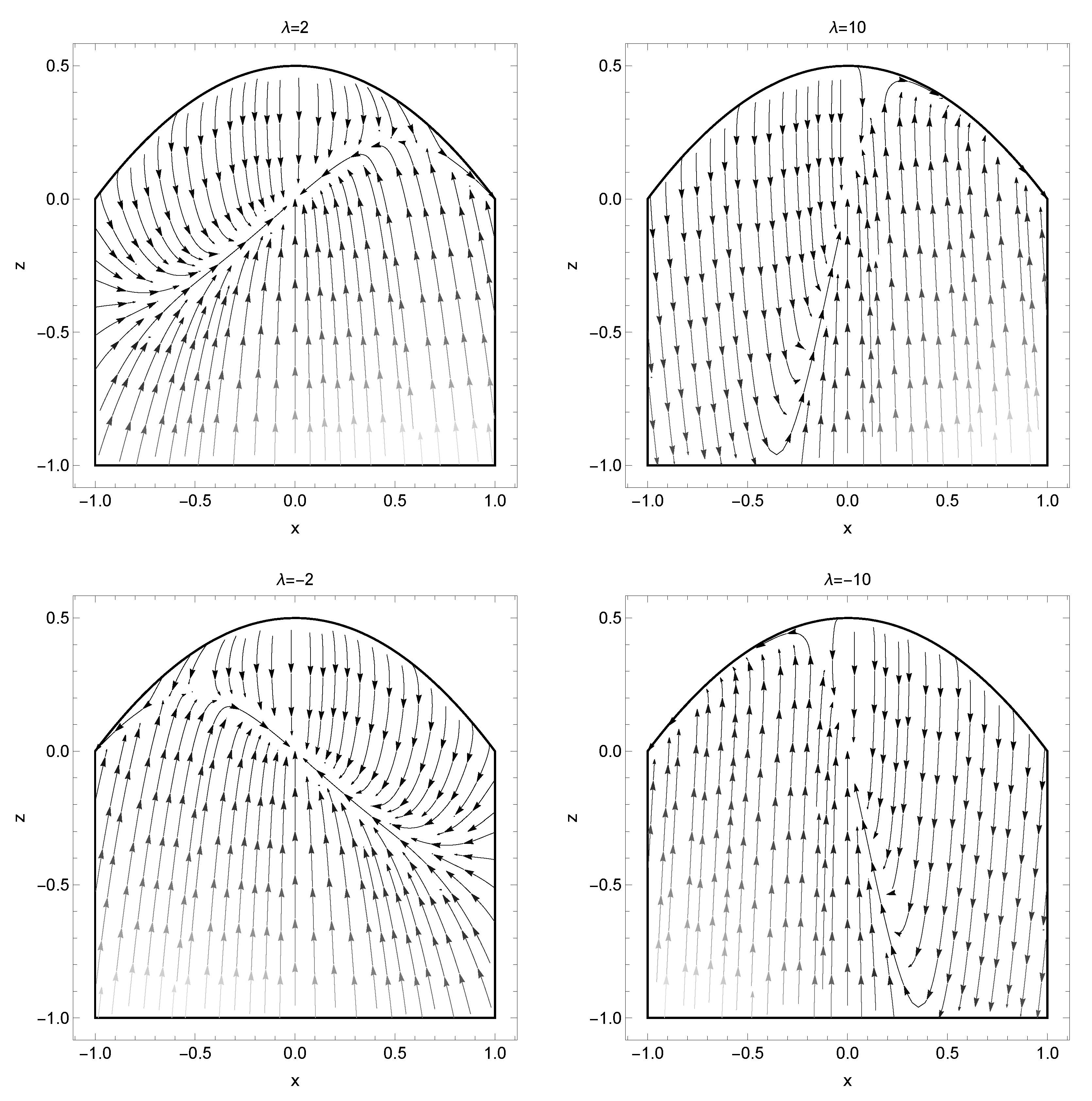
In Figure 1, Figure 2 and Figure 3 we present phase-portraits in the two- and three-dimensional spaces for the dynamical system (22)–(25) for different values of parameter . From the plots, it is clear that the trajectories go in the area where ; this means that it seems that stationary points exist at the infinity regime. In the following analysis, specifically in Section 5, we study the existence of stationary points for very large values of .
Subcase
Consider the specific scenario where , and the scalar field potential assumes the role of the cosmological constant, i.e., .
The stationary points are and . Point characterizes the de Sitter solution with , and it consistently acts as an attractor due to the negative eigenvalues of the linearized system.
In Figure 4 we present the three-dimensional phase-space for the latter dynamical system with . We observe that is the future attractor of the dynamical system.
4.3. Case III: and
Let us assume now the case where and and .
For this cosmological model, we introduce the variables
Thus, the field equations are expressed by the following algebraic-differential system
and
The stationary points of the dynamical system (36)–(40) which satisfy the constraint Equation (35) are
where is a real solution of the algebraic equation
Points and are the extensions of points in for the nonconstant potential in the five-dimensional space. Point is new and describes a universe where potential contributes in the cosmological fluid. is real and physical, accepted for , that is, . The effective equation of state parameter . We observe that , which means that point can not describe acceleration. In Figure 5, the is given as it is presented in Equation (42).
We observe that in this case where contributes in the cosmological fluid there is not any stationary point which can describes inflation. We omit the presentation of the stability properties and we focus in the special case where .
The results of this Section are summarized in Table 1.
5. Analysis at Infinity
Until now we have seen that the de Sitter universe exists only for the asymptotic solutions with a constant, that is, . We have investigated the existence of asymptotic solutions at the finite regime; however, the dynamical variables are constrained by the algebraic equation , which means that they can take values at infinity. In order to study the existence of asymptotic solutions at infinity we should introduce Poincare variables.
In case II, we focus on and . We introduce the new variable , and the two-dimensional system in the plane reads
Indeed, there exist the stationary points with coordinates , and . Point is , while points and describe de Sitter solutions with and .
As far as the stability properties are concerned, the resulting eigenvalues for point are and for point we derive . We infer that is always a source and is always an attractor.
Because of the constraint equation , at the new stationary points we calculate and . Thus, point is the de Sitter solution described by point C in [37].
6. Conclusions
In this study, we conducted a thorough phase-space analysis of the cosmological model, considering different forms of the potential functions. Our findings indicate that the cosmological model does not exhibit the de Sitter universe as an attractor, except in the case where the potential function represents the cosmological constant. Specifically, we investigated the following cosmological scenarios for the two potential functions: (I) , , (II) , and (III) , .
Referring to Table 1, for the analysis at the finite regime, we observe that for Model I, two stationary points emerge, characterizing the era of matter dominance. In contrast, Model II, which involves an exponential potential, reveals three stationary points that pertain to matter-dominated epochs. This finding stands in contrast to the outcomes previously reported in [37,38]. However, in the scenario where the exponent becomes zero, leading to the cosmological constant limit, a de Sitter solution emerges. A natural question which arises is if there are other forms for the scalar field potential and in which the de Sitter universe exists as an asymptotic solution. For a general potential function parameter is not a constant but a dynamical parameter which satisfies the equation
Thus, the stationary points depend on the value of which solves the algebraic equation . Consequently, a de Sitter point exist when is a root of the algebraic equation . For the potential , it follows that which means that the algebraic equation reads , with solutions and . As a result, on the surface , the de Sitter point exist. On the other hand, for the power-law potential , it follows , and the algebraic equation reads , that is, the de Sitter solution exist. Of course the stability properties of the de Sitter solution depend on the function form of . It is important to note that the asymptotic solution with leads to a scalar field potential which remains constant.
For the third cosmological scenario, Model III, the absence of solutions capable of describing acceleration is notable. An exception is found only in the special case where . In this circumstance, a collection of stationary points corresponding to scaling solutions manifests. Although accelerated solutions are present, they do not provide a de Sitter universe at the finite regime.
However, because the dynamical variables of the field equations are not constrained, they can reach infinity. Specifically for Model II, we investigate the existence of stationary points when . We found that, at infinity, there exist two stationary points which correspond to two de Sitter solutions. The one solution is always a source, while the other is always an attractor.
The current investigation underscores the potency of phase-space analysis as a robust tool for assessing the viability of gravitational models and constraining proposed theories. Importantly, this analysis can also serve as a classification and selection rule for the initial value problem. For instance, Model II, for , has two attractors, one of the points and the stationary point . On the other hand, for , is the unique attractor, and the de Sitter universe is the unique future solution.
Funding
This work was partially financially supported by the National Research Foundation of South Africa (Grant Numbers 131604). The author thanks the support of Vicerrectoría de Investigación y Desarrollo Tecnológico (Vridt) at Universidad Católica del Norte through Núcleo de Investigación Geometría Diferencial y Aplicaciones, Resolución Vridt No—098/2022.
Data Availability Statement
No data available.
Conflicts of Interest
The author declares no conflict of interest.
References
- Persic, M.; Salucci, P.; Stel, F. The universal rotation curve of spiral galaxies—I. The dark matter connection. Mon. Not. R. Astron. Soc. 1996, 281, 27–47. [Google Scholar] [CrossRef]
- Weinberg, D.H.; Colombi, S.; Davé, R.; Katz, N. Baryon Dynamics, Dark Matter Substructure, and Galaxies. Astrophys. J. 2008, 678, 6. [Google Scholar]
- Riess, A.G.; Filippenko, A.V.; Challis, P.; Clocchiatti, A.; Diercks, A.; Garnavich, P.M.; Gilliland, R.L.; Hogan, C.J.; Jha, S.; Kirshner, R.P.; et al. Observational evidence from Supernovae for an accelerating universe and cosmological constant. Astron. J. 1998, 116, 1009. [Google Scholar]
- Tegmark, M. et al. [SDSS Collaboration] The 3D power spectrum of galaxies from the SDSS. Astrophys. J. 2004, 606, 702–740. [Google Scholar]
- Kowalski, M.; Rubin, D.; Aldering, G.; Agostinho, R.J.; Amadon, A.; Amanullah, R.; Balland, C.; Barbary, K.; Blanc, G.; Challis, P.J.; et al. Improved Cosmological Constraints from New, Old, and Combined Supernova Data Sets. Astrophys. J. 2008, 686, 749. [Google Scholar]
- Yoo, J.; Watanabe, Y. Theoretical models of dark energy. Int. J. Mod. Phys. D 2012, 21, 1230002. [Google Scholar]
- Clifton, T.; Ferreira, P.G.; Padilla, A.; Skordis, C. Modified Gravity and Cosmology. Phys. Rep. 2012, 513, 1–189. [Google Scholar]
- Nojiri, S.; Odintsov, S.D.; Oikonomou, V. Modified gravity theories on a nutshell: Inflation, bounce and late-time evolution. Phys. Rep. 2017, 692, 1–104. [Google Scholar]
- Ferraro, R.; Fiorini, F. Modified teleparallel gravity. Phys. Rev. D 2007, 75, 084031. [Google Scholar] [CrossRef]
- Paliathanasis, A. Dynamical analysis of f(Q) -cosmology. Phys. Dark Univ. 2023, 41, 101255. [Google Scholar]
- Krssak, M.; van den Hoogen, R.J.; Pereira, J.G.; Boehmer, C.G.; Coley, A.A. Teleparallel Theories of Gravity. Class. Quantum Grav. 2019, 36, 183001. [Google Scholar]
- Rani, S.; Jawad, A.; Bamba, K.; Malik, I.-U. Cosmological Consequences of New Dark Energy Models in Einstein-Aether Gravity. Symmetry 2019, 11, 509. [Google Scholar]
- Li, B.; Barrow, J.D.; Mota, D.F. Cosmology of modified Gauss-Bonnet gravity. Phys. Rev. D 2007, 76, 044027. [Google Scholar]
- Ratra, B.; Peebles, P.J.E. Cosmological consequences of a rolling homogeneous scalar field. Phys. Rev. D 1988, 37, 3406. [Google Scholar]
- Hordenski, G.W. Second-order scalar-tensor field equations in a four-dimensional space. Int. J. Theor. Phys. 1975, 10, 363–384. [Google Scholar]
- Socorro, J.; Pérez-Payán, S.; Hernández-Jiménez, R.; Espinoza-García, A.; Díaz-Barrón, L.R. Classical and quantum exact solutions for a FRW in chiral like cosmology. Class. Quantum Grav. 2021, 38, 135027. [Google Scholar]
- von Marttens, R.; Barbosa, D.; Alcaniz, J. One-parameter dynamical dark-energy from the generalized Chaplygin gas. J. Cosmol. Astropart. Phys. 2023, 2023, 052. [Google Scholar]
- Akrami, Y.; Sasaki, M.; Solomon, A.R.; Vardanyan, V. Multi-field dark energy: Cosmic acceleration on a steep potential. Phys. Lett. B 2021, 819, 136427. [Google Scholar]
- Mamon, A.A.; Paliathanasis, A.; Saha, S. An extended analysis for a generalized Chaplygin gas model. Eur. Phys. J. C 2022, 82, 232. [Google Scholar]
- Cardone, V.F.; Troisi, A.; Capozziello, S. Unified dark energy models: A phenomenological approach. Phys. Rev. D 2004, 69, 083517. [Google Scholar]
- Bento, M.C.; Bertolami, O.; Sen, A.A. Generalized Chaplygin gas, accelerated expansion, and dark-energy-matter unification. Phys. Rev. D 2009, 70, 083519. [Google Scholar] [CrossRef]
- Perrotta, F.; Matarrese, S.; Torki, M. Instability of Chaplygin gas trajectories in unified dark matter models. Phys. Rev. D 2004, 70, 121304. [Google Scholar] [CrossRef]
- Wu, Y.-B.; Li, S.; Lu, J.-B.; Yang, X.-Y. The modified Chaplygin gas as a unified dark sector model. Mod. Phys. Lett. A 2007, 22, 783–790. [Google Scholar] [CrossRef]
- Gorini, V.; Kamenshchik, A.Y.; Moschella, U.; Piattella, O.F.; Starobinsky, A.A. More about the Tolman-Oppenheimer-Volkoff equations for the generalized Chaplygin gas. Phys. Rev. D 2009, 80, 104038. [Google Scholar] [CrossRef]
- Zhu, Z.-H. Generalized Chaplygin gas as a unified scenario of dark matter/energy: Observational constraints. Astron. Astrophys. 2004, 423, 421–426. [Google Scholar]
- Li, B.; Barrow, J.D. Does bulk viscosity create a viable unified dark matter model? Phys. Rev. D 2009, 79, 103521. [Google Scholar]
- Atreya, A.; Bhatt, J.R.; Mishra, A.K. Viscous self interacting dark matter cosmology for small redshift. J. Cosmol. Astropart. Phys. 2019, 2019, 045. [Google Scholar]
- Bertacca, D.; Matarrese, S.; Pietroni, M. Unified Dark Matter in Scalar Field Cosmologies. Mod. Phys. Lett. A 2007, 22, 2893–2907. [Google Scholar]
- Bertacca, D.; Bartolo, N.; Matarrese, S. Unified Dark Matter Scalar Field Models. Adv. Astron. 2010, 2010, 904379. [Google Scholar]
- Paliathanasis, A. Dynamics of Chiral Cosmology. Class. Quantum Grav. 2020, 37, 195014. [Google Scholar]
- Leon, G.; Paliathanasis, A.; Saridakis, E.N.; Basilakos, S. Unified dark sectors in scalar-torsion theories of gravity. Phys. Rev. D 2022, 106, 024055. [Google Scholar] [CrossRef]
- Amendola, L. Coupled quintessence. Phys. Rev. D 2000, 62, 043511. [Google Scholar] [CrossRef]
- Wetterich, C. An asymptotically vanishing time-dependent cosmological “constant”. Astron. Astrophys. 1995, 301, 321. [Google Scholar]
- Di Valentino, E.; Melciorri, A.; Mena, O.; Pan, S.; Yang, W. Interacting Dark Energy in a closed universe. Mon. Not. R. Astron. Soc. Lett. 2021, 502, L23–L28. [Google Scholar] [CrossRef]
- Bonilla, A.; Kumar, S.; Nunes, R.C.; Pan, S. Reconstruction of the dark sectors’ interaction. Mon. Not. R. Astron. Soc. 2022, 512, 4231–4238. [Google Scholar] [CrossRef]
- Benisty, D.; Guendelman, E.I. Interacting diffusive unified dark energy and dark matter from scalar fields. Eur. Phys. J. C 2017, 77, 396. [Google Scholar] [CrossRef]
- Benisty, D.; Guendelman, E.I. Unified dark energy and dark matter from dynamical spacetime. Phys. Rev. D 2018, 98, 023506. [Google Scholar] [CrossRef]
- Anagnostopulos, F.K.; Benisty, D.; Basilakos, S.; Guendelman, E.I. Dark energy and dark matter unification from dynamical space time: Observational constraints and cosmological implications. J. Cosmol. Astropart. Phys. 2019, 2019, 003. [Google Scholar] [CrossRef]
- Gonzales, T.; Leon, G.; Quiros, I. Dynamics of quintessence models of dark energy with exponential coupling to dark matter. Class. Quantum Grav. 2006, 23, 3165. [Google Scholar] [CrossRef]
- Tot, J.; Yildirim, B.; Coley, A.; Leon, G. The dynamics of scalar-field Quintom cosmological models. Phys. Dark Univ. 2023, 39, 101155. [Google Scholar] [CrossRef]
- Millano, A.D.; Leon, G.; Paliathanasis, A. Global dynamics in Einstein-Gauss-Bonnet scalar field cosmology with matter. Mathematics 2023, 11, 1408. [Google Scholar] [CrossRef]
- Coley, A.A.; van den Hoogen, R.J. Dynamics of multi-scalar-field cosmological models and assisted inflation. Phys. Rev. D 2000, 62, 023517. [Google Scholar] [CrossRef]
- Amendola, L.; Gannouji, R.; Polarski, D.; Tsujikawa, S. Conditions for the cosmological viability of f(R) dark energy models. Phys. Rev. D 2007, 75, 083504. [Google Scholar] [CrossRef]
- Khyllep, W.; Dutta, J.; Saridakis, E.N.; Yesmakhanova, K. Cosmology in f(Q) gravity. Phys. Rev. D 2023, 107, 044022. [Google Scholar] [CrossRef]
- Gao, C.; Kunz, M.; Liddle, A.R.; Parkinson, D. Unified dark energy and dark matter from a scalar field different from quintessence. Phys. Rev. D 2010, 81, 043520. [Google Scholar] [CrossRef]
- Guendelman, E.I.; Kaganovich, A.B. Dark energy, dark matter and fermion families in the two measures theory. Int. J. Mod. Phys A 2004, 19, 5325–5332. [Google Scholar] [CrossRef]
- Guendelman, E.I.; Kaganovich, A.B. Exotic Low Density Fermion States in the Two Measures Field Theory: Neutrino Dark Energy. Int. J. Mod. Phys. A 2006, 21, 4373–4406. [Google Scholar] [CrossRef]
- Gronwald, F.; Muench, U.; Macias, A.; Hehl, F.W. Volume elements of spacetime and a quartet of scalar fields. Phys. Rev. D 1998, 58, 084021. [Google Scholar] [CrossRef]
- Comelli, D. A Way to Dynamically Overcome the Cosmological Constant Problem. Int. J. Mod. Phys. A 2008, 23, 4133–4143. [Google Scholar] [CrossRef]
- Guendelman, E.I. Gravitational Theory with a Dynamical Time. Int. J. Mod. Phys. A 2010, 15, 4081–4099. [Google Scholar] [CrossRef]
Figure 1.
Phase-space portraits of the dynamical system (22), (25) on the two-dimensional planes , and for and .
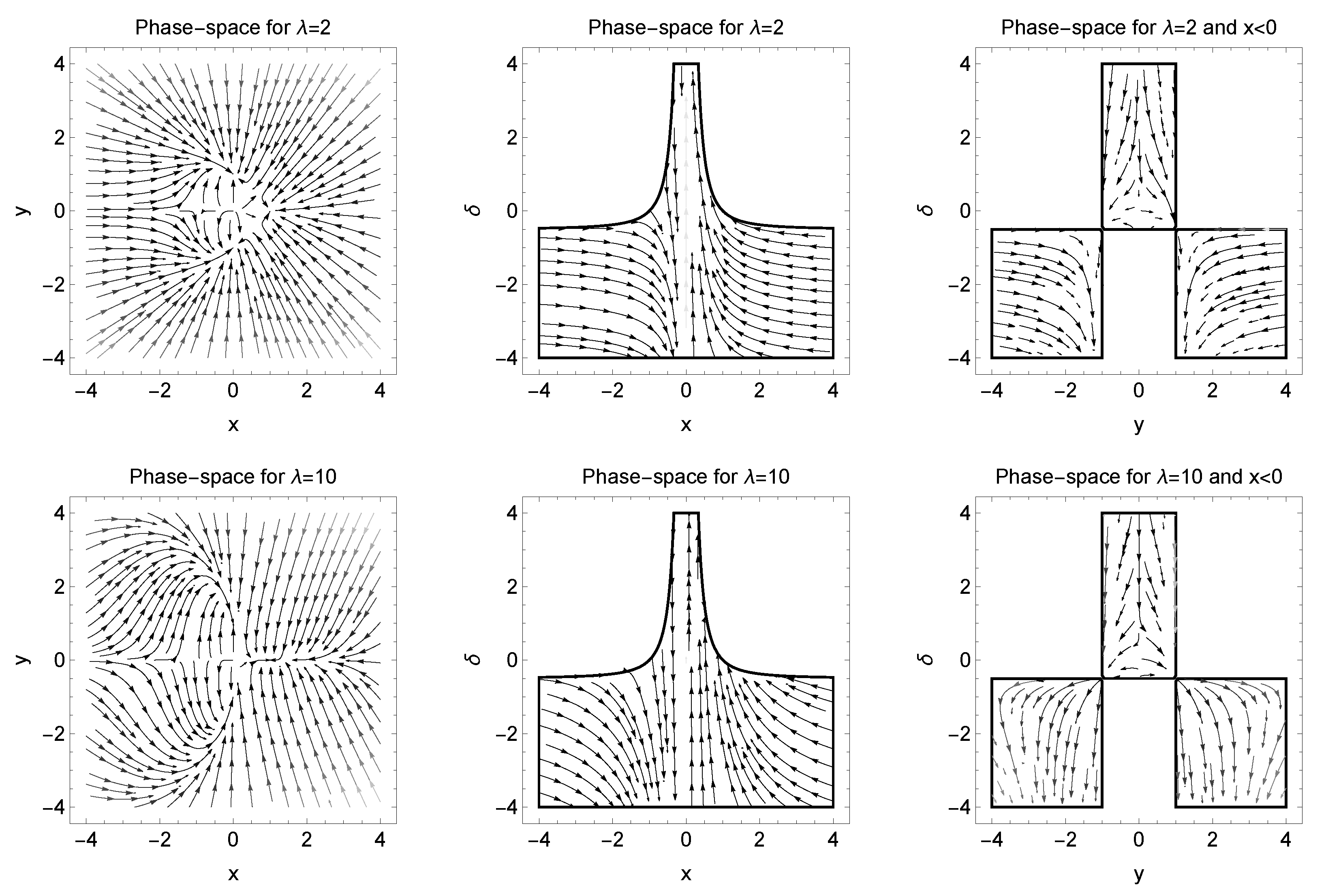
Figure 2.
Phase-space portraits of the dynamical system (22), (25) on the two-dimensional planes , and for and .

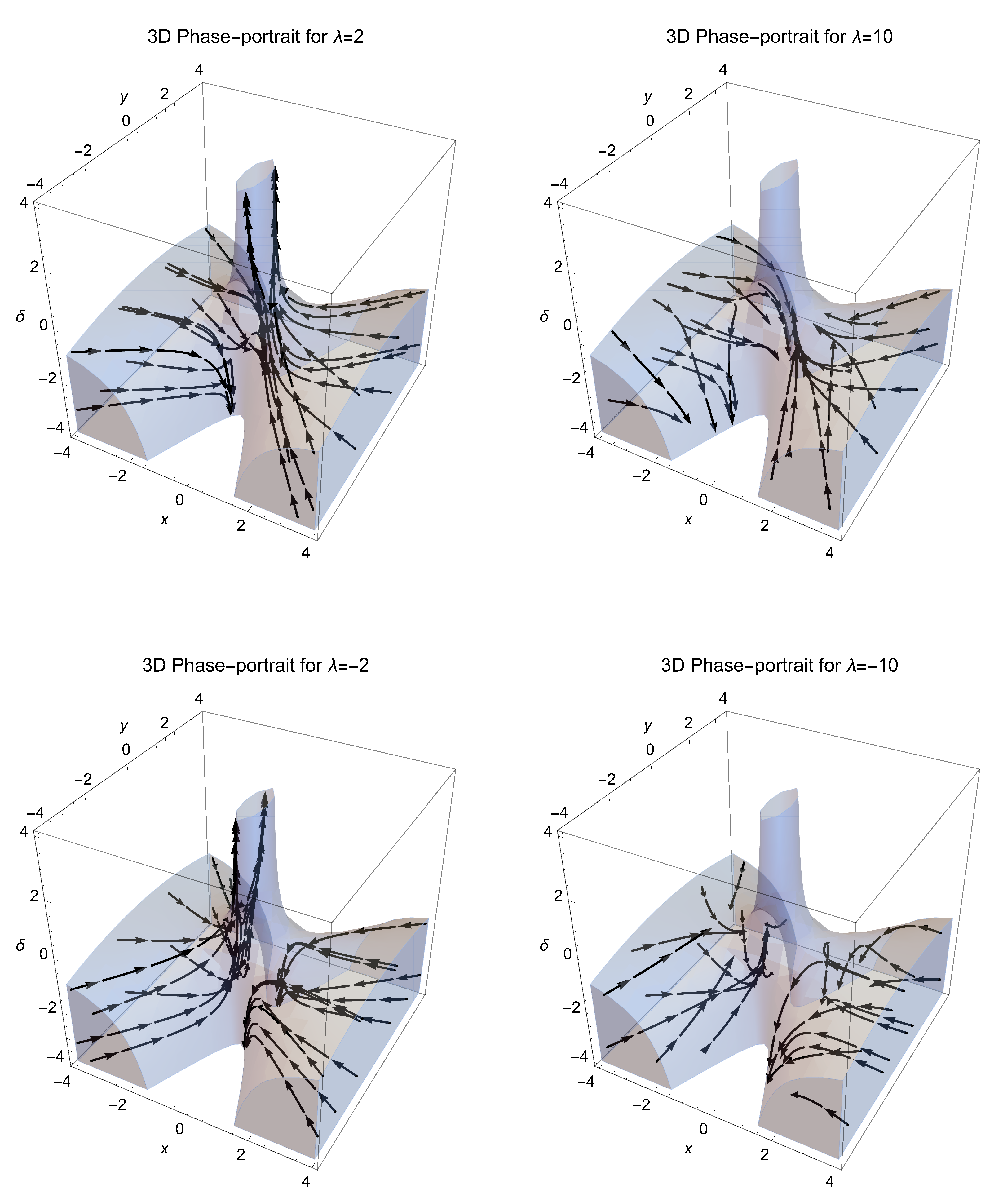
Figure 4.
3D phase-space portraits of the dynamical system (22), (25) for , where is the unique attractor.
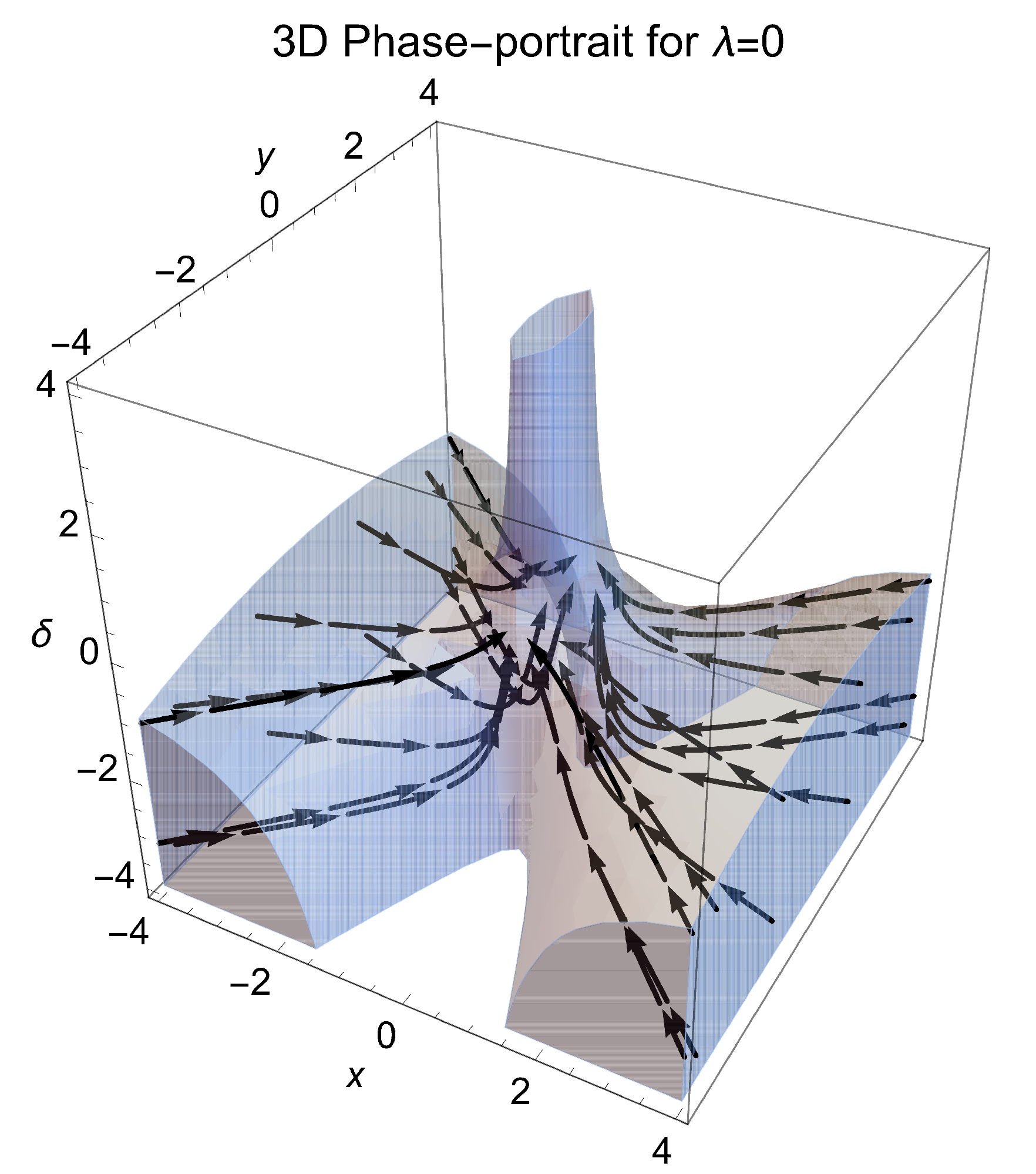
Figure 5.
We plot the as it is given by the algebraic equation .
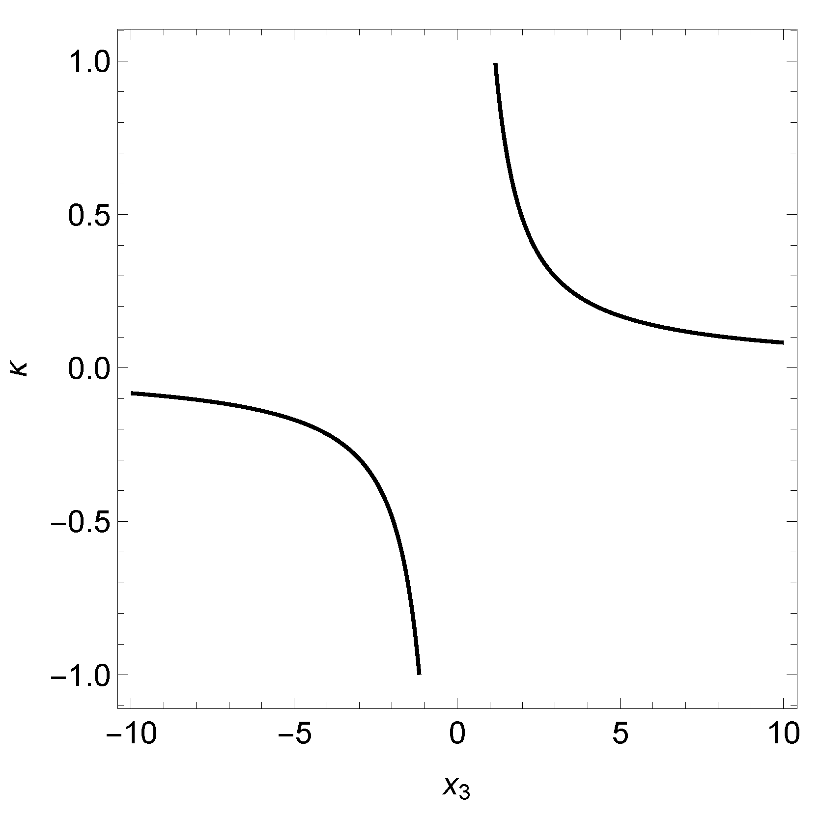
Figure 6.
Phase-space portraits of the dynamical system (43), (44) on the two-dimensional planes for , and .
Figure 6.
Phase-space portraits of the dynamical system (43), (44) on the two-dimensional planes for , and .

Table 1.
Stationary points and physical properties at the finite regime.
| Model | Point | Acceleration? | |||
|---|---|---|---|---|---|
| I | 0 | ||||
| 0 | No | ||||
| II | |||||
| 0 | No | ||||
| 0 | No | ||||
| II | |||||
| 0 | No | ||||
| Yes | |||||
| III | |||||
| 0 | No | ||||
| 0 | No | ||||
| No |
Disclaimer/Publisher’s Note: The statements, opinions and data contained in all publications are solely those of the individual author(s) and contributor(s) and not of MDPI and/or the editor(s). MDPI and/or the editor(s) disclaim responsibility for any injury to people or property resulting from any ideas, methods, instructions or products referred to in the content. |
© 2023 by the author. Licensee MDPI, Basel, Switzerland. This article is an open access article distributed under the terms and conditions of the Creative Commons Attribution (CC BY) license (https://creativecommons.org/licenses/by/4.0/).
Share and Cite
MDPI and ACS Style
Paliathanasis, A. Revise the Phase-Space Analysis of the Dynamical Spacetime Unified Dark Energy Cosmology. Universe 2023, 9, 406. https://doi.org/10.3390/universe9090406
AMA Style
Paliathanasis A. Revise the Phase-Space Analysis of the Dynamical Spacetime Unified Dark Energy Cosmology. Universe. 2023; 9(9):406. https://doi.org/10.3390/universe9090406
Chicago/Turabian StylePaliathanasis, Andronikos. 2023. "Revise the Phase-Space Analysis of the Dynamical Spacetime Unified Dark Energy Cosmology" Universe 9, no. 9: 406. https://doi.org/10.3390/universe9090406
Note that from the first issue of 2016, this journal uses article numbers instead of page numbers. See further details here.