The Statistics of Primordial Black Holes in a Radiation-Dominated Universe: Recent and New Results

Abstract

We review the nonlinear statistics of Primordial Black Holes that form from the collapse of over-densities in a radiation-dominated Universe. We focus on the scenario in which large over-densities are generated by rare and Gaussian curvature perturbations during inflation. As new results, we show that the mass spectrum follows a power law determined by the critical exponent of the self-similar collapse up to a power spectrum dependent cutoff, and that the abundance related to very narrow power spectra is exponentially suppressed. Related to this, we discuss and explicitly show that both the Press–Schechter approximation and the statistics of mean profiles lead to wrong conclusions for the abundance and mass spectrum. Finally, we clarify that the transfer function in the statistics of initial conditions for Primordial Black Holes formation (the abundance) does not play a significant role.

1. Setup

Primordial Black Holes (PBHs), if they exist, are arguably the most economical form of Dark Matter. A PBH is the final state of a large over-density collapse that happened long before matter–radiation equality. A black hole is surely of a primordial origin if its mass is lower than the solar one. In the realm in which PBHs account for all of Dark Matter, this is precisely where their masses need to be [1].

Assuming only the standard model of particle physics, before matter–radiation equality and after inflation the universe is in a state dominated by radiation. Because black holes only interact gravitationally, they behave as dust particles. In other words, in a homogeneous and isotropic universe (i.e., a Friedman–Robertson–Walker (FRW) universe) with metric element

$$d{s}^2=-d{t}^2+a{\left(t\right)}^{2}d\overrightarrow{x}·d\overrightarrow{x},$$

(1)

the energy density of radiation scales as $a^{-4}$ and that of Primordial Black Holes scales as $a^{-3}$. In the minimal scenario in which the perturbations in the mean FRW universe were seeded by inflation, large over-densities might only have been generated at scales much smaller than those related to the cosmic microwave background radiation observed today. Thus, for a high reheating temperature PBHs will have had a long period to increase their energy density relatively to radiation. In this scenario, the initial density of PBHs is tiny; therefore, the formation of a PBH represents a rare event. This has a particular resonance with the theory of inflation, as inflation mainly generates perturbative over-densities. However, because perturbations are quantum in nature, their amplitudes are statistically distributed, meaning that non-perturbative over-densities can be generated as well, albeit rarely.

Thus far, there is no evidence of (perturbative) deviations from the simple Gaussian statistics; therefore, for the purposes of discussion, we assume it here in order to investigate the statistics of PBH formation from a given Gaussian-distributed initial seed of curvature perturbations. Our procedure can be generalized to other distributions as well.

Before moving on, it is necessary to quickly review the conditions for PBH formation in an expanding universe. Interested readers may consult the review of [2] for a more technical perspective; here, we provide a more intuitive overview.

In the hoop conjecture of Thorne [3], a black hole forms if a portion of fluid with “mass” M in an asymptotically flat spacetime can be enclosed within a hoop of perimeter $2\pi R_s$, where $R_s\equiv 2M$ ($G_N=\hslash =c=1$) is the Schwarzschild radius of the portion of that fluid. For a fluid of density $\rho$, we can define an instantaneous mass ($dt=0$) as

$$M{|}_{dt=0}\equiv 4\pi {\int }_0^R\rho {\overline{R}}^{2}d\overline{R}{|}_{dt=0},$$

(2)

where we have assumed that the energy density of the fluid is isotropic and R is the areal radius. In an expanding universe, this mass is known as the Misner–Sharp mass (MS) [4]. The scenario we are interested in here is a localized large over-density (defined in a specific gauge that we clarify later on) evolving in a homogeneous and isotropic radiation-dominated universe. Because of the assumption of asymptotic flatness in the hoop conjecture, we could attempt to obtain similar conditions in an expanding universe by subtracting the infinitely long wavelength mode (the background energy density) from the MS mass. Thus, we define the instantaneous over-mass as

$$\delta M\left(R\right){|}_{dt=0}\equiv 4\pi {\int }_0^R\delta \rho {\overline{R}}^{2}d\overline{R}{|}_{dt=0},$$

(3)

where $\delta \rho \equiv \rho -{\rho }_b$ is the over-density with respect to the background ${\rho }_b$.

The extension of the hoop conjecture to an expanding universe would then be that a collapse into a black hole starts at position $R_{BH}$ whenever

$$\mathcal{C}{|}_{dt=0}\equiv \frac{2\delta M\left(R_{BH}\right){|}_{dt=0}}{R_{BH}}{|}_{dt=0}\sim 1.$$

(4)

We can now remove the fixed time and define

$$\mathcal{C}(r,t)\equiv \frac{8\pi {\int }_0^r\delta \rho R{(\overline{r},t)}^2{\partial }_{\overline{r}}R(\overline{r},t)d\overline{r}}{R(r,t)},$$

(5)

where r is the radial coordinate of the general isotropic metric

$$d{s}^2=-A{(r,t)}^{2}d{t}^2+\frac{{\partial }_{r}R{(r,t)}^{2}d{r}^2}{\Gamma {(r,t)}^2}+R{(r,t)}^{2}d{\Omega }_2^2.$$

(6)

The metric function $\Gamma$ is the “boost factor” of the fluid (being 1 for vanishing fluid velocity and gravitational mass [4]); thus, the Misner–Sharp mass is the equivalent of the “rest mass” of the fluid. The function $\mathcal{C}$, defined in Equation (5), was called the compaction function in [5], in which the compaction factor was defined without the factor 2. The factor 2 was introduced in [6] to resemble the Schwarzschild potential; see [7] for the latest interpretations of the earlier work of [5]. In the same paper, it was shown that, in agreement with the hoop conjecture, a black hole would inexorably form whenever $\mathcal{C}\sim 1$.

Let us now return to our primordial black hole scenario. We have already mentioned that whenever PBHs are generated by large inflationary perturbations during the radiation epoch they are generically rare. Assuming a Gaussian distribution of perturbations, this implies an approximate spherical symmetry around the peak of such rare large perturbations [8]. Thus, in this regime the condition for collapse into black holes can be provided in terms of $\mathcal{C}$:

The first trapped horizon is formed at a radius equaling the maximum of the compaction function [6]; in other words, a black hole will form at a scale $r=r_{\mathrm{BH}}\left(t_{\mathrm{BH}}\right)$ solution of ${\partial }_r\mathcal{C}=0$ whenever $\mathcal{C}(r_{\mathrm{BH}},t_{\mathrm{BH}})\sim 1$. The threshold for PBH formation can then be provided in terms of a critical value ${\mathcal{C}}_c(r_m\left(t_i\right),t_i)$, where $t_i\ne t_{\mathrm{BH}}$ is some initial time [6,9].

Initial Conditions and Threshold

The question we answer in this section is:

Under which initial conditions for $\mathcal{C}$ will a BH form at some later time $t=t_{\mathrm{BH}}$?

Under the inflationary paradigm, perturbations set in at scales larger than the cosmological horizon. On such scales and at the leading order in gradient expansion, the metric (6) can always be recast (see, e.g., [10] for a review) into a local FRW metric:

$$d{s}_l^2\simeq -d{t}_l^2+a_l{\left(t_l\right)}^{2}d{r}_l^2+r_l^2{a}_l{\left(t_l\right)}^{2}d{\Omega }_2^2$$

(7)

where the subscript l refers to local coordinates and functions and $a_l\left(t\right)$ to the spatial rescaling due to a long-wavelength perturbation, i.e., a perturbation with a wavelength larger than the cosmological horizon of the background. Up to decaying terms, we find that $a_l\left(t_l\right)\simeq a\left(t_l\right)$, where a is the background scale factor in local time [11].

The idea is then to find appropriate initial conditions for $\mathcal{C}$ at super-horizon scales such that a future black hole would form. At the leading order in gradient expansion, however, the compaction function vanishes, making it necessary to go beyond this concept.

If the typical co-moving scale of the perturbation is $r_0$, then we can define the parameter

$$\sigma \left(t\right)\equiv \frac{R_H{\left(t\right)}^2}{R_p{\left(t\right)}^2}=\frac{a_i^2}{H^{2}a{\left(t\right)}^2{r}_0^2}=\frac{a_i^2}{\dot{a}{\left(t\right)}^2{r}_0^2}\ll 1,$$

(8)

where $a_i$ is the scale factor at some initial time $t_i$. Thus, $R(t_i,r)=ra\left(t_i\right)$.

If we specialize to the case of radiation,

$$\sigma \left(t\right)=\frac{3\frac{a{\left(t\right)}^2}{a_i^2}}{\left(l_p^4{\rho }_0\right){(r_0/l_p)}^2},$$

(9)

where ${\rho }_0$ is the background energy-density at $t=t_i$, then we have now replaced units by using $l_p$ as the Planck scale. Because the universe is expanding, a necessary condition is then to choose an initial time such that

$$l_p^4{\rho }_0\gg \frac{l_p^2}{r_0^2{a}_i^2}.$$

(10)

As already anticipated, a generic spherically symmetric metric can be recast in the following diagonal form:

$$d{s}^2=-A{(r,t)}^{2}d{t}^2+\frac{{\partial }_{r}R{(r,t)}^2}{1-K(r,t)r^2}d{r}^2+R{(r,t)}^{2}d{\Omega }_2^2.$$

(11)

At super-horizon scales, we can then expand each function in (11) in powers of $\sigma \left(t\right)$ [12,13]. However, it turns out that the zeroth order in $\sigma$ is ambiguous, and we might instead write [14]

$$1-K(r,t)r^2=(1-K_i\left(r\right)r^2)\tilde{K}(r,t),$$

(12)

where $K_i\left(r\right)$ is the curvature K at an initial time $t=t_i$ where the perturbation is at super-horizon scales and $\tilde{K}(r,t)=1+{\sum }_{n=1}^{\infty }{\tilde{K}}_n\left(r\right)\sigma {\left(t\right)}^n$. For consistency, K should then be the next-to-leading order in gradient expansion; and indeed, we find that $K_i\sim \mathcal{O}(l_p^2/r_0^2)$ [14] when scales smaller than the horizon are cut off.

With this, at the leading order in $\sigma$ (though fully nonlinearly) we finds that for the case of radiation we have [6,15]

$$\mathcal{C}\simeq \frac{2}{3}{K}_i\left(r\right)r^2.$$

(13)

As can be seen, at super-horizon scales the compaction function is approximately constant. Thus, a black hole can only be formed when the typical scale of the perturbation re-enters the horizon. This typical scale, as we explain, is related to the size $r_m$ in which the compaction function is maximal. Moreover, as it is found numerically [6], the co-moving location of this maximum does not change much up to the moment in which the hoop conjecture conditions are met. Thus, we shall henceforth approximate it as constant.

Our prescription for the black hole formation is then that a black hole eventually forms whenever $\mathcal{C}$ at its maximum is larger than a certain critical value ${\mathcal{C}}_c$, which we specify later on. The constant(s) ${\mathcal{C}}_c$ are called the “thresholds”.

The curvature $K_i$ is related to the initial co-moving over-density as follows [6]:

$$a_i^2\delta {\rho }_i\left(r\right)\propto (K_i+\frac{r}{3}{K}_i^{\prime })$$

(14)

where $f^{\prime }\equiv {\partial }_{r}f$ for a given function f. At the maximum of the compaction function $r=r_m$, where we want to define a threshold for the black hole formation, we have

$$\mathcal{C}\left(r_m\right)\propto \delta {\rho }_i\left(r_m\right)r_m^2.$$

(15)

Therefore, the threshold on the compaction function greatly differs from other previous prescriptions, which considered a “threshold” of the over-density amplitude at its peak $r\sim 0$. Here, we mean a radius small enough to be closer to the highest point of the over-density while being large enough to retain the super-horizon approximation.. In the presence of an over-density it is clear that $r_m\ne 0$, as $\mathcal{C}\ge 0$; thus, the relationship between $\delta \rho \left(0\right)$ and $\mathcal{C}\left(r_m\right)$ depends on the full profile of the over-density, and any statistics based on the distribution of $\delta {\rho }_i\left(0\right)$ are limited to very specific statistical realizations. We return to this point later on.

The initial spatial metric at time $t=t_i$ and at super-horizon scales is then

$$d{s}^2{|}_{t=t_i}\simeq \frac{a_i^{2}d{r}^2}{1-K_i\left(r\right)r^2}+a_i^2{r}^{2}d{\Omega }_2^2$$

(16)

recalling that $R(t_i,r)=a_{i}r$. However, inflationary initial conditions are usually phrased using a different conformal form

$$d{s}^2{|}_{t=t_i}\simeq a_i^2{e}^{2\zeta \left(\widehat{r}\right)}\left(d{\widehat{r}}^2+{\widehat{r}}^{2}d{\Omega }_2^2\right),$$

(17)

where $\zeta$ is the curvature perturbation in the synchronous gauge. For both expressions to be the same, it must be the case that both

$$r=e^{\zeta \left(\widehat{r}\right)}\widehat{r}\mathrm{and}\frac{dr}{\sqrt{1-K_i\left(r\right)r^2}}=e^{\zeta \left(\widehat{r}\right)}d\widehat{r}.$$

(18)

However, the expression on the left implies that $dr/d\widehat{r}=e^{\zeta \left(\widehat{r}\right)}[1+\widehat{r}{\partial }_{\widehat{r}}\zeta \left(\widehat{r}\right)]$; along with the expression on the right, this implies that

$$K_i\left(r\right)r^2=1-{\left[1+\widehat{r}{\partial }_{\widehat{r}}\zeta \left(\widehat{r}\right)\right]}^2.$$

(19)

In the $\widehat{r}$ coordinates, the maximum of the compaction function is at that $\widehat{r}={\widehat{r}}_m$ where ${\partial }_{\widehat{r}}\left(\widehat{r}{\partial }_{\widehat{r}}\zeta \right)=0$; due to the regularity condition $K_i\left(r\right)r^2<1$, the amplitude of this maximum cannot exceed $2/3$.

As for the over-density, it is obvious that the threshold ${\mathcal{C}}_c$ cannot be generically written in terms of the value of $\zeta$ at its central peak unless strong assumptions are made concerning the statistical realizations of $\zeta$. Moreover, because the theory is invariant under shifts of $\zeta$ at super-horizon scales, its peak value only has a meaning by fixing it at certain scales. In contrast, the value of the compaction function at its maximum is an observable. Previous attempts at statistical descriptions of PBH formations have assumed that the spread of the curvature profile around the mean is negligible [16,17,18]. Following [19], we instead scan all possible compaction function shapes, defining the corresponding threshold for each realization.

2. Analytic Formula for the Threshold

As we have discussed earlier, a gravitational collapse occurs at positions where the maximum of the compaction function is over threshold. The threshold is that value of the compaction function for which a black hole of mass zero is eventually formed. Far away from the maximum the fluid is dispersed away, whereas close to the center the regularity of the curvature $K\left(r\right)$ requires the compaction function to decay as $r^2$. Therefore, what matters most for the threshold is the form of the compaction function around its maximum. Moreover, because the conditions to form a black hole are tied to the local gradient pressures, the threshold only approximately depends on the local shape of the compaction function. At the maximum ($r=r_m$), we can then fit the compaction function using its value $\mathcal{C}\left(r_m\right)$ and its normalized curvature $q\equiv \frac{-r_m^2{\mathcal{C}}^{″}\left(r_m\right)}{4\mathcal{C}\left(r_m\right)}$ [20]; see [21] for other equations of state.

In [20], the following fitting function was used:

$${\mathcal{C}}_{fit}\left(r\right)=\mathcal{C}\left(r_m\right)\frac{r^2}{r_m^2}{e}^{\frac{1}{q}(1-{\left[\frac{r}{r_m}\right]}^{2q})},$$

(20)

where $\mathcal{C}\left(r_m\right)$, $r_m$, and q are calculated from the compaction function of the perturbation.

The average of the fitting function

$$\overline{\mathcal{C}}\left(r\right)=\frac{3}{r_m^3}\theta (r-r_m){\int }_0^{r_m}{\mathcal{C}}_{fit}\left(r^{\prime }\right)r^{\prime 2}d{r}^{\prime }$$

(21)

would then be a fictitious top-hat compaction function which has a threshold for radiation equal to ${\overline{\mathcal{C}}}_c=\frac{2}{5}$[9]. With this, by inverting (21) we can obtain the threshold for $\mathcal{C}\left(r_m\right)$ [20]:

$${\mathcal{C}}_c\left(q\right)=\frac{4}{15}{e}^{-\frac{1}{q}}\frac{q^{1-\frac{5}{2q}}}{\Gamma \left(\frac{5}{2q}\right)-\Gamma (\frac{5}{2q},\frac{1}{q})}.$$

(22)

Note that ${\mathcal{C}}_c\ge \frac{2}{5}$; this lower bound has been confirmed by numerical studies. Numerical simulations show that the critical value (22) and its dependence on q are accurate to within 2% [20].

If (22) is provided in terms of derivatives with respect to $\widehat{r}$ rather than r, e.g., in [22], then

$$q=\frac{-{\widehat{r}}_m^2{\partial }_{\widehat{r}}^2\mathcal{C}\left({\widehat{r}}_m\right)}{4\mathcal{C}\left({\widehat{r}}_m\right)(1-\frac{3}{2}\mathcal{C}\left({\widehat{r}}_m\right))}.$$

(23)

With this analytical formula for the threshold of PBH formation, we are now in a position to calculate the statistical abundance of PBHs in our universe.

3. The Statistics of Compaction Function

A scalar field (in particular, the inflaton) does not have a preferred direction; therefore, we expect isolated perturbations to be spherical. This symmetry is broken only by the interference of two or more nearby perturbations [8]. Thus, focusing on rare events, as in the case of PBHs formed during the radiation era, it is the case that spherical symmetry around a rare peak of a Gaussianly distributed amplitude is well preserved.

The observed cosmological curvature perturbations at the cosmic microwave background (CMB) scale are extremely close to (multivariate) Gaussian [23]. We assume that this is true on all scales. Nevertheless, it should be noted by the reader that for most of the inflationary evolution related to PBH formation, e.g., [24,25,26], this assumption may be too strong, e.g., [27,28,29].

In the Gaussian case, then, as discussed above, we have

$$\mathcal{C}(\widehat{r},{\overrightarrow{x}}_0)=\frac{2}{3}\left[1-{(1+\widehat{r}{\partial }_{\widehat{r}}\zeta (\widehat{r},{\overrightarrow{x}}_0))}^2\right],$$

(24)

where $x_0$ defines the center of the spherical distribution and $\widehat{r}=\parallel \overrightarrow{x}-\overrightarrow{x_0}\parallel$ in the coordinates (17). Although the combination $\widehat{r}{\partial }_{\widehat{r}}\zeta (\widehat{r},{\overrightarrow{x}}_0)$ is independent on the choice of radial units, $\widehat{r}$ is not.Therefore, we fix the scale factor at matter–radiation equality $a_{eq}=1$ such that $\widehat{r}$ represents physical distances.

Before developing the full statistics in detail, it is interesting to note that even if $\zeta$ (and its derivatives) are multi-Gaussian distributed, $\mathcal{C}$ follows a non-centrally peaked multi-${\chi }^2$ distribution. Thus, rare configurations of $\mathcal{C}$ generically do not coincide with rare configurations of $\zeta$.

PBHs are then distributed according to the multi-${\chi }^2$-statistics of $\mathcal{C}$ constrained under the following conditions:

There is a center: $\mathcal{C}(\widehat{r},\overrightarrow{x})$ has a peak, and there exists a position ${\overrightarrow{x}}_0$ such that

$$\overrightarrow{\nabla }\mathcal{C}(\widehat{r},\overrightarrow{x}){|}_{\overrightarrow{x}={\overrightarrow{x}}_0}=0,\mathrm{and},{\nabla }^2\mathcal{C}(\widehat{r},\overrightarrow{x}){|}_{\overrightarrow{x}={\overrightarrow{x}}_0}<0.$$

(25)

This condition is studied in peaks theory [8]. At this level, we can already see that the statistics we are looking for are very different from the Press–Schechter/excursion set approach from [30,31], which is often used in the literature. Whereas peaks theory seeks to describe the point process which describes the positions around which collapse occurs, the Press–Schechter calculation does not describe a point process; it only aims at a statistical description of the mass fraction in bound objects. It returns biased (incorrect) estimates of this mass fraction, as it assumes that this can be done by considering the statistics of all positions in space [32] rather than the special subset of positions around which collapse occurs [33]. This point has been discussed extensively in the literature on halo formation during matter domination [32,33,34]; because essentially all of that discussion remains relevant during radiation domination, we do not repeat it here.)

$\mathcal{C}(\widehat{r},{\overrightarrow{x}}_0)$ has a maximum at $\widehat{r}={\widehat{r}}_m$: this condition is verified for

$${\partial }_{\widehat{r}}\mathcal{C}(\widehat{r},{\overrightarrow{x}}_0){|}_{\widehat{r}={\widehat{r}}_m}=0,\mathrm{and},{\partial }_{\widehat{r}}^2\mathcal{C}(\widehat{r},{\overrightarrow{x}}_0){|}_{\widehat{r}={\widehat{r}}_m}<0.$$

(26)

This important condition appeared for the first time in the nonlinear statistics of [19], and is based on the excursion set peaks formalism from [34]. In our statistics, we calculate the probability that the compaction function has a maximum for a given scale r, thereby scanning all possible realizations of $\mathcal{C}$. Other proposed statistics [16,17,18] have instead considered only the maximum associated with the averaged profile. This difference is crucial. Using our procedure, we are able to associate a threshold for each statistical realization of the perturbation’s shapes (or the above q variable) instead of considering only the statistics of ${\mathcal{C}}_c$ for a fixed (presumably average!) q.

$\mathcal{C}({\widehat{r}}_m,{\overrightarrow{x}}_0)$ is over the threshold: the condition in this case is

$$\mathcal{C}({\widehat{r}}_m,{\overrightarrow{x}}_0)\ge {\mathcal{C}}_c\left(q\right).$$

(27)

Again, this condition crucially differs from those employed in [16,17,18], with respectively considered thresholds for the co-moving curvature and for the over-density at the peak (i.e., at $r=0$).

3.1. The Statistical Variables and the Role of the Transfer Function

As we have already commented, a direct connection to inflation is obtained by considering $\zeta \left(\overrightarrow{x}\right)$ as the main statistical variable. Strictly speaking, this is the curvature perturbation calculated in the past infinity as if radiation was always dominating the universe’s evolution [6] (in the language of [6], in the limit of $t\to 0$). Practically, however, numerical simulations start at a finite time from the cosmological singularity. Thus, one would be tempted to consider the statistics of PBHs at the time $t_{BH}$, at which the maximum of the compaction function crosses the cosmological horizon (e.g., [22,35,36]), where nonlinear effects start to play a crucial role. The statistics would then be developed by hoping that the evolution of $\zeta$, via the perturbative transfer function, would retain its invariant Gaussian nature up to the point of crossing the horizon. However, it is expected that the time evolution of curvature perturbations in the nonlinear regime would badly break our assumption of Gaussianity. For example, in the context of stochastic inflation, the nonlinear regime is no longer Markovian [11].

Even accepting the assumption of Gaussianity, because the perturbation at $t=t_{BH}$ is outside the regime of validity of gradient expansion the use of $\zeta (r_m,t_{BH})$ is not consistent with the quasi-homogeneous initial conditions of the Misner–Sharp system [14], which really use $\zeta \left(\overrightarrow{x}\right)\equiv \zeta (\overrightarrow{x},t\to 0)$. Thus, using $\zeta (\overrightarrow{x},t_{BH})$ would mean setting a different numerical problem from the one studied in the literature [6,9]. In turn, this choice would lead to a background-dependent threshold which cannot be obtained as a simple generalization of the one employed here (the threshold suggested in [22] tries to generalize the one in [20] using the transfer function in the definition of the compaction function maximum; however, as we have discussed in the text this is inconsistent).

Thus, we accept the small error caused by not being able to run the simulation from the infinite past, and consider the initial conditions for black hole formation at the leading order in gradient expansion. This error is smaller than the error we already accepted by using our analytical formula for the threshold. One can appreciate it by looking at the simulated Hamiltonian constraint deviation caused by the use of quasi-homogeneous conditions at a finite time [9].

Having defined the relevant variable, we are now equipped to study its statistical proprieties. In Fourier space, we have

$$\zeta \left(\overrightarrow{x}\right)=\int \frac{d^{3}k}{{\left(2\pi \right)}^3}{e}^{i\overrightarrow{k}·\overrightarrow{x}}{\zeta }_k,$$

(28)

where the ${\zeta }_k$s modes, assumed to be Gaussian, coincide with the Fourier modes of the curvature perturbations in synchronous gauge and at the leading order in gradient expansion. More precisely, the amplitudes follow a Rayleigh distribution and the phases a uniform distribution.

While the curvature perturbation is a function of $\overrightarrow{x}$, $\mathcal{C}$ is a function of $\widehat{r}$ and ${\overrightarrow{x}}_0$. Thus, we need to specify the meaning of $\widehat{r}{\partial }_{\widehat{r}}\zeta (\widehat{r},{\overrightarrow{x}}_0)$; we can integrate the Laplacian of $\zeta$ over a ball B centered on ${\overrightarrow{x}}_0$, obtaining (henceforth, we drop the hats)

$${\int }_B{d}^{3}x{\nabla }^2\zeta =4\pi r^2{\partial }_r\zeta (r,{\overrightarrow{x}}_0),$$

(29)

where we have assumed spherical symmetry around ${\overrightarrow{x}}_0$ (having in mind a rare peak from inflation). The same relation can be written as

$$r{\partial }_r\zeta (r,{\overrightarrow{x}}_0)=\frac{1}{4\pi r}\int d^{3}x{\nabla }^2\zeta \theta \left(r-\parallel \overrightarrow{x}-{\overrightarrow{x}}_0\parallel \right).$$

(30)

Using the Fourier decomposition (28), we obtain

$$r{\partial }_r\zeta (r,{\overrightarrow{x}}_0)=-\frac{1}{4\pi r}\int \frac{d^{3}k}{{\left(2\pi \right)}^3}{k}^2{\zeta }_k\int d^{3}x{e}^{i\overrightarrow{k}·\overrightarrow{x}}\theta \left(r-\parallel \overrightarrow{x}-{\overrightarrow{x}}_0\parallel \right).$$

(31)

For the second integral, we can use polar coordinates:

$$\int d^{3}x{e}^{i\overrightarrow{k}·\overrightarrow{x}}\theta \left(r-\parallel \overrightarrow{x}-{\overrightarrow{x}}_0\parallel \right)=2\pi e^{i\overrightarrow{k}·{\overrightarrow{x}}_0}\int d\overline{r}d\varphi {\overline{r}}^2{e}^{ik\overline{r}cos\varphi }\theta \left(r-\parallel \overrightarrow{x}-{\overrightarrow{x}}_0\parallel \right)=e^{i\overrightarrow{k}·{\overrightarrow{x}}_0}\frac{4\pi }{k^3}\left(-krcos\left(kr\right)+sin\left(kr\right)\right)$$

allowing us to use the suggestive form

$$r{\partial }_r\zeta =\frac{1}{3}\int \frac{d^{3}k}{{\left(2\pi \right)}^3}{e}^{i\overrightarrow{k}·{\overrightarrow{x}}_0}{\left(kr\right)}^2{\zeta }_k{W}_{\mathrm{TH}}\left(kr\right),$$

(32)

where we have used the definition of the Fourier-transformed top-hat window function

$$W_{\mathrm{TH}}\left(kr\right)=3\frac{sin\left(kr\right)-krcos\left(kr\right)}{{\left(kr\right)}^3}.$$

(33)

We stress here that the top-hat window function was not added by hand, and is simply encoded in the variable $r{\partial }_r\zeta$. However, this appearance of $W_{\mathrm{TH}}$ ensures that sub-horizon modes of $r{\partial }_r\zeta$ (for r larger than the cosmological horizon size) are cut away, a necessary condition for the initial conditions of the Misner–Sharp equations. Evidently, then, in order to construct the compaction function we ought to be interested in the Laplacian of the curvature perturbation.

This Laplacian is related to the linear density perturbation used in previous statistics [16]. Hence, for greater intuitiveness we can define the new variable as

$$g_r\left({\overrightarrow{x}}_0\right)\equiv -\frac{4}{3}r{\partial }_r\zeta =-\frac{4}{9}\int \frac{d^{3}k}{{\left(2\pi \right)}^3}{e}^{i\overrightarrow{k}·{\overrightarrow{x}}_0}{\left(kr\right)}^2{\zeta }_k{W}_{\mathrm{TH}}\left(kr\right).$$

(34)

Note that $g_r$ is a linear combination of ${\zeta }_k$, meaning that it similarly follows a Gaussian statistics.

Although the compaction function is fully nonlinear, for greater intuitiveness it should be noted that $g_r\left({\overrightarrow{x}}_0\right)$ is the would-be smoothed linear over-density on a ball of radius r at super-horizon scales. This results from the Poisson equation of linear perturbations in an FRW Universe. It should be stressed here that this linear over-density is only an auxiliary (i.e., non-physical) function in the regime that we are interested in.

With $g_r\left({\overrightarrow{x}}_0\right)$, we can now write the compaction function as

$$\mathcal{C}(r,{\overrightarrow{x}}_0)=g_r\left({\overrightarrow{x}}_0\right)\left(1-\frac{3}{8}{g}_r\left({\overrightarrow{x}}_0\right)\right).$$

(35)

Finally, note that when we impose that the condition that ${\overrightarrow{x}}_0$ must be a maximum, the coordinates can be shifted to locally fix ${\overrightarrow{x}}_0=\overrightarrow{0}$.

3.2. Statistical Conditions I: Existence of Isolated Peaks

In what follows, we search for a special center ${\overrightarrow{x}}_0={\overrightarrow{x}}_p$ which is a peak for the compaction function. Indeed, as already discussed, the first constraint to form a PBH is the existence of an isolated peak in the compaction function which defines the spatial center of the approximately spherically symmetric initial over-density (again, we are assuming rare peaks). Then, we need to restrict the statistical realizations of the compaction function to those that fulfill the constraints

$${\overrightarrow{\nabla }}_{{\overrightarrow{x}}_0}\mathcal{C}(r,{\overrightarrow{x}}_0)=0\mathrm{and}{\nabla }_{{\overrightarrow{x}}_0}^2\mathcal{C}(r,{\overrightarrow{x}}_0)<0.$$

(36)

The first condition identifies positions which are extremes, while the second ensures that these extremes are local maxima, i.e., peaks.

The condition for an extreme of $\mathcal{C}$ is satisfied either where ${\overrightarrow{\nabla }}_{\overrightarrow{x}}{g}_r\left({\overrightarrow{x}}_0\right)=0$ or where $g_r\left({\overrightarrow{x}}_0\right)=4/3$; however, as the latter has probability zero and would produce a PBH of negligible mass, we discard it here. It can now be seen that the condition for the peak of the compaction function is the same condition for an extreme of the linear over-density, as considered earlier in [16]. This extreme is a maximum whenever $0<g_r\left({\overrightarrow{x}}_0\right)<4/3$ and a minimum for $4/3<g_r\left({\overrightarrow{x}}_0\right)<8/3$. The first region corresponds to the so-called type I collapse and the second to type II [37]. Although type II has yet to be thoroughly explored, it is believed that such peaks collapse rapidly [38]. However, because high peaks are extremely rare and type IIs are even rarer than type Is, we only consider type Is in what follows (i.e., $g_r\left({\overrightarrow{x}}_0\right)\le 4/3$). Moreover, because $g_r$ must exceed $0.49$ for PBH formation (corresponding to the limit ${\mathcal{C}}_c\ge 0.4$ [20]), the conditions for the existence of an (isolated) center of the compaction function are

$$0.49\lesssim g_r\left({\overrightarrow{x}}_p\right)\le \frac{4}{3},{\overrightarrow{\nabla }}_{\overrightarrow{x_p}}{g}_r\left(\overrightarrow{x_p}\right)=0,\mathrm{and}{\nabla }_{{\overrightarrow{x}}_p}^2{g}_r\left({\overrightarrow{x}}_p\right)<0.$$

(37)

In a discretized sense (see [8]), the total number density of peaks is

$$n_{peaks}=\sum _{{\overrightarrow{x}}_p}{\delta }^{\left(3\right)}(\overrightarrow{x}-{\overrightarrow{x}}_p);$$

(38)

the idea is to use the statistical variable $g_r$ and its derivatives instead of the peak(s) position(s).

We can expand $g_r$ around the maximum(s) (${\overrightarrow{x}}_p$):

$$g_r\left(\overrightarrow{x}\right)\simeq g_r\left({\overrightarrow{x}}_p\right)+\frac{1}{2}{\nabla }_i{\nabla }_j{g}_r\left({\overrightarrow{x}}_p\right)(x^i-x_p^i)(x^j-x_p^j).$$

(39)

Defining $\overrightarrow{\eta }\left(\overrightarrow{x}\right)\equiv \overrightarrow{\nabla }{g}_r\left(\overrightarrow{x}\right)$ and ${\chi }_{ij}\equiv {\nabla }_i{\nabla }_j{g}_r\left(\overrightarrow{x_p}\right)$, we have

$$n_{peaks}=\sum _{{\overrightarrow{x}}_p}\left|\det {\chi }_{ij}\right|{\delta }^{\left(3\right)}\left(\overrightarrow{\eta }\right),$$

(40)

where we have used the position around the peak ${\eta }_i\left(\overrightarrow{x}\right)\simeq {\sum }_j{\chi }_{ij}{(\overrightarrow{x}-{\overrightarrow{x}}_p)}^j$.

The sum over peaks can now be replaced by the probability of having a peak in a position ${\overrightarrow{x}}_p$. As already discussed, we assume that $\zeta$, and consequently $g_r$, follow multi-Gaussian distributions. By this we mean that $\zeta$ is the anti-Fourier transformation of the Gaussian random variables ${\zeta }_k$. While the probability distribution we look for is a Gaussian on $g_r\left(\overrightarrow{x}\right)$, as we have discussed, concerning the peaks it is enough to use second-order expansion $g_r$ around the peak value and consider $p\left(g_r\left(\overrightarrow{x}\right)\right)\to p(g_r\left({\overrightarrow{x}}_p\right),{\chi }_{ij},\overrightarrow{\eta }\left({\overrightarrow{x}}_p\right))$.

Statistically, vector, scalar, and tensor quantities can decouple; thus, $p(g_r,{\chi }_{ij},\overrightarrow{\eta })=$ $p\left(g_r\right)p\left({\chi }_{ij}^T\right)p\left({\chi }_r\right|g_r)p\left(\overrightarrow{\eta }\right)$, where ${\chi }^T$ is the traceless part of the Hessian matrix of $g_r$. We additionally define ${\chi }_r\equiv -r^2{\nabla }^2{g}_r\left({\overrightarrow{x}}_p\right)$, which is the trace part of the Hessian. The latter is a scalar, and as such correlates with $g_r$. All of these probabilities obviously remain multi-Gaussians.

Then, the mean number of peaks is

$$n_{peaks}\to \int d{\chi }_{ij}d\overrightarrow{\eta }d{g}_r\left|\det {\chi }_{ij}\right|{\delta }^{\left(3\right)}\left(\overrightarrow{\eta }\right)\theta \left({\chi }_r\right)p\left(g_r\right)p\left({\chi }_{ij}^T\right)p\left({\chi }_r\right|g_r)p\left(\overrightarrow{\eta }\right),$$

(41)

where the Dirac delta and the Heaviside theta define ${\overrightarrow{x}}_p$ as an extreme that is a maximum.

The Dirac delta constraint is easy to integrate:

$$\int d\overrightarrow{\eta }{\delta }^{\left(3\right)}\left(\overrightarrow{\eta }\right)p\left(\overrightarrow{\eta }\right)\to \frac{1}{{\left(2\pi \right)}^{3/2}{\sigma }_{\eta }^3},$$

(42)

where the third power is due to the fact that the distribution is three-dimensional and ${\sigma }_{\eta }\equiv \sqrt{\det \left(\langle {\eta }_i{\eta }_j\rangle \right)}$.

The integral in ${\chi }_{ij}^T$ is more involved. However, assuming an approximate rotation invariance (we consider high and rare peaks), the determinant of the Hessian simply provides the normalized trace value to the cube, i.e., $\left|\det {\chi }_{ij}\right|\sim \frac{{\chi }_r^3}{r^3}$, while the integral over $d{\chi }^T$ only provides the variance. All in all, then, we have

$$\int d{\chi }_{ij}\left|\det {\chi }_{ij}\right|p\left({\chi }_{ij}\right)\theta \left({\chi }_r\right)\sim {\int }_0^{\infty }d{\chi }_r\frac{{\sigma }_{\chi }^3{\chi }_r^3}{r^3}p\left({\chi }_r\right|g_r).$$

(43)

The exact integration in ${\chi }^T$ can actually be done exactly, leading to

$$n_{peaks}=\int d{g}_r{\int }_0^{\infty }d{\chi }_r\frac{f({\chi }_r/{\sigma }_{\chi })}{{\left(2\pi r_{*}^2\right)}^{3/2}}p\left(g_r\right)p\left({\chi }_r\right|g_r),$$

(44)

where the explicit calculation to find $f\left(x\right)$ (from the integration in ${\chi }^T$) can be found in appendix A of [8] The function is

$$f\left(x\right)=\frac{x^3-3x}{2}\left[\mathrm{erf}\left(\sqrt{\frac{5}{2}}x\right)+\mathrm{erf}\left(\sqrt{\frac{5}{2}}\frac{x}{2}\right)\right]+\sqrt{\frac{2}{5\pi }}\left[\left(\frac{31x^2}{4}+\frac{8}{5}\right)e^{-5x^2/8}+\left(\frac{x^2}{2}-\frac{8}{5}\right)e^{-5x^2/2}\right],$$

(45)

and, as anticipated, $f\left(x\right)\to x^3$ for $x\to \infty$ (i.e., large isolated peaks); finally, $r_{*}\equiv r{\sigma }_{\eta }/{\sigma }_{\chi }$.

We pause here for a moment. The integral in $g_r$ has been intentionally left indefinite, for the reason that only a subset of peaks that are the maximum of the compaction function and over-threshold are related to PBH formation. Because we are looking for rare configurations, we assume the existence of only one maximum per peak, thereby discarding the cloud-in-cloud possibility. In this respect, a local maximum would be a global one. A new condition, that $r=r_m$ must be a maximum, should then be supplemented in the statistics of peaks, which is what we do in the next section.

3.3. Statistical Conditions II: Maximum of Compaction Function

The second constraint we must impose is the existence of a maximum for the compaction function. Here, note that ‘maximum’ refers to the variation of r, rather than the variation of the spatial position $\overrightarrow{x}$, meaning that when the spatial peak position $\overrightarrow{x_p}$ has been found the maximum can be related to the behavior of the derivatives of $\mathcal{C}$ with respect to r. Thus, what we really want to count is

$$\frac{d{n}_{peaks\cap max}}{dr}=\sum _{{\overrightarrow{x}}_p,r_m}\delta (\overrightarrow{x}-{\overrightarrow{x}}_p)\delta (r-r_m),$$

(46)

where $r_m$ denotes the compaction function maximum for each ${\overrightarrow{x}}_p$, where we have assumed that a peak and a maximum of the compaction function do not happen at more than one smoothing scale.

As before, for type I black holes the maxima of $\mathcal{C}$ coincide with those of $g_r\left({\overrightarrow{x}}_0\right)$; hence, we can consider the following expansion around $r_m$:

$$\frac{d{g}_r}{dr}=\frac{d{g}_r}{dr}{|}_{r_m}+\frac{d^2{g}_r}{d{r}^2}{|}_{r_m}(r-r_m)+\dots =\frac{d^2{g}_r}{d{r}^2}{|}_{r_m}(r-r_m)+\dots .$$

(47)

In what follows, it is useful to define the following dimensionless quantities related to expansion in r:

$$v_r\equiv r\frac{d{g}_r}{dr},w_r\equiv -r^2\frac{d^2{g}_r}{d{r}^2},\mathrm{and}{\chi }_r\equiv -r^2{\nabla }^2{g}_r.$$

(48)

The curvature of the compaction function is actually related to the Hessian around the peak; indeed, we have

$$2g_r+w_r=-\frac{4}{9}\int \frac{d^{3}k}{{\left(2\pi \right)}^3}{e}^{i\overrightarrow{k}·{\overrightarrow{x}}_0}{\left(kr\right)}^4{\zeta }_k{W}_{\mathrm{TH}}\left(kr\right)={\chi }_r.$$

(49)

This shows that for the variables associated with the ‘infinite’ past (i.e., ${\chi }_r$, the (dimensionless) Laplacian of $g_r$, and $w_r$), the second derivative with respect to scale the r differs by $2g_r$, i.e., the curvatures with respect to position and scale (${\chi }_r$ and $w_r$, respectively) differ by $2g_r$.

With the above definitions, we have

$$v_r=-w_{r_m}\frac{(r-r_m)}{r_m}+\dots ,$$

(50)

thus, we have

$$\delta (r-r_m)=\frac{w}{r_m}\delta \left(v_r\right)\sim \frac{w}{r_m}\delta \left(v_{r_m}\right)$$

(51)

whenever the Dirac delta is imposed. The density of these states is then obtained by replacing the following in (44):

$$p\left(g_r\right)d{g}_r\to p(g_{r_m},v_{r_m},w)d{v}_{r_m}dwd{g}_{r_m}.$$

(52)

By changing the sum in $r_m$ into an integral, we finally obtain the number of peaks per unit volume having a maximum at some r (we now remove for simplicity all the indices r):

$$n_{peaks\cap max}={\int }_{r_{min}}^{r_{max}}\frac{dr}{r}{\int }_0^{\infty }d\chi {\int }_0^{\infty }dww\int dg\frac{f(\chi /{\sigma }_{\chi })}{{\left(2\pi r_{*}^2\right)}^{3/2}}p(g,v=0,w)p\left(\chi \right|g,v=0,w)\theta \left(\chi \right)$$

(53)

where the integral over only positive values of w specifies that $r_m$ is a maximum.

Because $\chi =2g+w$, i.e., $\chi$ is completely determined by g and w, $p\left(\chi \right|g,v=0,w)\to \delta (\chi -(2g+w))$; thus, we finally obtain

$$n_{peaks\cap max}={\int }_{r_{min}}^{r_{max}}\frac{dr}{r}{\int }_0^{\infty }dww\int dg\frac{f(\chi /{\sigma }_{\chi })}{{\left(2\pi r_{*}^2\right)}^{3/2}}p(g,v=0,w),$$

(54)

where one should read $\chi =2g+w$. Note that because both w and g are positive we do not need to add an extra constraint for the maximum in ${\overrightarrow{x}}_p$ (i.e., $\theta \left({\chi }_r\right)$).

The integral in r requires further explanation. First of all, the minimal radius should be larger than the Hubble radius at the initial time in order for the gradient expansion to be valid. Second, because of Hawking evaporation, black holes less massive than $\approx {10}^{15}gr$ will have completely evaporated by now, and should not be counted [1]. Thus (replacing Planck units $M_p\simeq 2\times {10}^{-5}gr$), because $M_{•}\sim M_p^2{H}_r^{-1}=ra\left(t_r\right)M_p^2$, we fix

$$r_{min}=\mathrm{MAX}\left[{\left(\frac{{10}^{12}gr}{M_p^2}\right)}^{3/4}{H}_{eq}^{-1/4},{\left(H\left(t_i\right)a\left(t_i\right)\right)}^{-1}\right],$$

(55)

where we have used $a_{eq}=1$ and $H_{eq}$ is the Hubble scale at matter equality. Whether the Hubble radius at initial conditions or the Hawking evaporation limit ought to be considered as the minimal radius depends on the specific inflationary model under investigation.

Similarly, the maximal scale we are interested in here is the Horizon size at matter–radiation equality:

$$r_{max}=H_{eq}^{-1}.$$

(56)

Finally, note that the integral in r is really the integral of all configurations that have a maximum for the compaction function for a given smoothing scale r; hence, we remove the sub-index m from now on.

3.4. Statistics Condition III: Being over the Threshold

We are now finally in a position to implement the over-threshold condition for the integral in $g_r$. Converse to the case of finding a local maximum for the compaction function, in general the threshold value is nonlocal, i.e., it depends on the profile realization of $g_r$ at all smoothing scales. Thus, the number of peaks we are looking for is the subset of $n_{peaks\cap max}$ such that for any possible smoothing scale configuration with the same peak position and same $r_m$ the corresponding $g_{r_m}$ is over-threshold. Obviously, this would lead to an untreatable computational problem.

To bypass this issue, previous approaches have considered only the mean $g_r$ profile [16] (here, we remind the reader that $g_r$ happens to equal the would be linear over-density [19]), and have consequently associated $r_m$ with the location of the compaction function maximum when the mean profile is used. However, unless all possible realizations of $g_r$ for any smoothing scale r have negligible spread from $\langle g_r\rangle$, this peak counting will be grossly wrong (similar arguments have been made for the $\zeta$ statistics in [17,18]). Here, we instead adopt the more refined argument already outlined in the introduction.

Although it is true that the threshold at the maximum of the compaction function depends upon the full $g_r$ profile [6], to a very good approximation the threshold only depends on the curvature of the compaction function around a maximum $r_m$[20]. Thus, we can simply consider the ensemble of all possible compaction function curvatures for any given smoothing scale $r=r_m$, then associate a threshold with each of these.

The realization of this condition requires some algebra; in the region $g\le \frac{4}{3}$ and at the maximum, we have

$$-r^2{\partial }_r^2\mathcal{C}{|}_{r=r_m}=-r^2{\partial }_r^2{g}_r\left(1-\frac{3}{4}{g}_r\right){|}_{r=r_m}=w\sqrt{1-\frac{3}{2}{\mathcal{C}}_c}.$$

(57)

leading to

$$q=\frac{w}{4{\mathcal{C}}_c\left(q\right)\sqrt{1-\frac{3}{2}{\mathcal{C}}_c\left(q\right)}},$$

(58)

and implying that ${\mathcal{C}}_c\left(q\right)={\mathcal{C}}_c\left(q\left(w\right)\right)={\mathcal{C}}_c\left(w\right)$. On the other hand, the threshold in terms of g is

$$g_c\left(w\right)=\frac{4}{3}\left(1-\sqrt{1-\frac{3}{2}{\mathcal{C}}_c\left(w\right)}\right)$$

(59)

Thus, the number density of peaks that would eventually collapse into Primordial Black Holes is

$$n_{•}={\int }_{r_{min}}^{r_{max}}\frac{dr}{r}{\int }_0^{\infty }dww{\int }_{g_c\left(w\right)}^{\frac{4}{3}}dg\frac{f(\chi /{\sigma }_{\chi })}{{\left(2\pi r_{*}^2\right)}^{3/2}}p(g,v=0,w).$$

(60)

3.5. Energy Density in PBHs

Super-horizon over-threshold perturbations that enter the horizon at the time $ra\left(t_r\right)=H{\left(t_r\right)}^{-1}$ quickly collapse into black holes (here, we assume instantaneous formation) [6]. Up to a deviation of about $\Delta \mathcal{C}\equiv \mathcal{C}-{\mathcal{C}}_c\sim {10}^{-2}$ from the threshold value [9], the mass is distributed according to the following scaling law [39]:

$$M_{•}=\frac{\mathcal{K}}{2H_r}{\left[\mathcal{C}\left(g\right)-{\mathcal{C}}_c\left(w\right)\right]}^{0.36},$$

(61)

where $H_r\equiv H\left(t_r\right)$. The function $\mathcal{K}$ is of $\mathcal{O}\left(1\right)$, and depends on the specific curvature profile chosen; thus, it depends slightly on r. Nevertheless, we keep it constant in our estimation of abundance, accepting the related error $\mathcal{O}\left(1\right)$. To fix its value, we take the typical value $\mathcal{K}\simeq 6$ from [9].

For $\Delta \mathcal{C}\ge {10}^{-2}$, the mass distribution starts to deviate from the scaling law with a maximum deviation of $\sim 15\%$[40]. Because the error on using (61) is on a similar order as that emerging from fixing $\mathcal{K}$, we keep it and retain the scaling law throughout.

Because we are interested in the energy density of PBHs at matter–radiation equality, we need to be careful about the evolution of the number density. Thus far, we have calculated the number density per co-moving volume. When black holes are formed, as we have already mentioned in the introduction, their energy density simply dilutes as dust, i.e., as the inverse of the volume expansion. At super-horizon scales and the leading order in gradient expansion, the power spectrum is constant; thus, peak positions in co-moving volumes do not change, i.e., at the leading order there are no intrinsic velocities between peaks. Obviously, at the next-to-leading order in gradient expansion this would not exactly be the case. While we do not consider this subtlety further here, we do mention that it would be incorrect to try to capture the intrinsic velocities between peaks by considering a linear transfer function in the statistics, for similar reasons as those outlined before in the case of threshold definition. More specifically, the transfer function capturing the time evolution of the power spectrum at linear order (even assuming that Gaussianity is not broken at next-to-leading order in gradients), is next to the leading order in gradient expansion. Therefore, considering a transfer function in the statistical correlators would imply the necessity of considering both new nonlinear thresholds and new nonlinear initial conditions. What should be done instead is to calculate the initial number density in co-moving volumes as done here, then simulate the velocity dispersion of the initial peaks at later times. We are not aware of any of such numerical simulation to date; thus, we accept the small related error in order to consider only the leading order in gradient expansion.

Having made these remarks, the total energy density of PBHs at matter–radiation equality is

$$\frac{d^2{\rho }_{•}}{drd{M}_{•}}\sim \sum _{{\overrightarrow{x}}_0,r_m,M_{•},\mathcal{C}\left(r_m\right)>{\mathcal{C}}_c}\delta (\overrightarrow{x}-{\overrightarrow{x}}_0)\delta (r-r_m)\delta \left(M_{•}-\frac{\mathcal{K}}{2H_r}{\left[\mathcal{C}\left(g\right)-{\mathcal{C}}_c\left(w\right)\right]}^{0.36}\right)M_{•}$$

(62)

or

$${\rho }_{•}={\int }_{r_{min}}^{r_{max}}\frac{dr}{r}{\int }_0^{\infty }dww{\int }_{g_c\left(w\right)}^{\frac{4}{3}}dg\frac{f(\chi /{\sigma }_{\chi })}{{\left(2\pi r_{*}^2\right)}^{3/2}}p(g,v=0,w)\frac{\mathcal{K}}{2H_r}{\left[\mathcal{C}\left(g\right)-{\mathcal{C}}_c\left(w\right)\right]}^{0.36},$$

(63)

where we have again set $a_{eq}=1$. We can now define the fractional density of PBHs at equality, ${\beta }_{•}\equiv \frac{{\rho }_{•}}{{\rho }_{eq}}$, as follows:

$$\begin{array}{cc}\hfill {\beta }_{•}& =\frac{8\pi }{3H_{eq}^2}{\int }_{r_{min}}^{r_{max}}\frac{dr}{r}{\int }_0^{\infty }dww{\int }_{g_c\left(w\right)}^{\frac{4}{3}}dg\frac{f(\chi /{\sigma }_{\chi })}{{\left(2\pi r_{*}^2\right)}^{3/2}}p(g,v=0,w)\frac{\mathcal{K}}{2H_r}{\left[\mathcal{C}\left(g\right)-{\mathcal{C}}_c\left(w\right)\right]}^{0.36}\hfill \\ \hfill & =\frac{4\pi \mathcal{K}}{3{\left(H_{eq}{r}_{eq}\right)}^3}{\int }_{r_{min}}^{r_{max}}\frac{dr}{r}\frac{{(r/r_{eq})}^2}{{(r/r_{eq})}^3}{\int }_0^{\infty }dww{\int }_{g_c\left(w\right)}^{\frac{4}{3}}dg\frac{f(\chi /{\sigma }_{\chi })}{{\left[2\pi {(r_{*}/r)}^2\right]}^{3/2}}p(g,v=0,w){\left[\mathcal{C}\left(g\right)-{\mathcal{C}}_c\left(w\right)\right]}^{0.36}.\hfill \end{array}$$

(64)

recalling that $H_{eq}{r}_{eq}=a_{eq}^{-1}$ and $a_{eq}=1$ in our units.

The final expression makes it easy to see that the abundance of PBHs with respect to radiation grows with the scale factor from formation. If we ignore the scaling solution and only focus on order of magnitudes, i.e., we consider that the PBH mass is provided simply by the mass within the horizon at formation, then we can ignore the integrals over w and g in the mass while retaining the dependence on r. Then, because $\mathcal{K}/\left(2H_r\right)\propto r^2$ and ${\left(2\pi r_{*}^2\right)}^{3/2}\propto r^3$, we find that we obtain $r_{\mathrm{eq}}/r=a_{eq}/a\left(t_r\right)$ for each r. This is the scaling we should expect; the integrals over w and g serve to return the actual fraction of patches which produce PBHs, and the fact that they depend on r shows how the energy density that is stored in PBHs builds up over time, i.e., as r increases.

3.6. Mass Spectrum of PBHs

The mass distribution per proper volume (known as the ‘mass function’) is

$$\frac{d{n}_{•}\left(M_{•}\right)}{d{M}_{•}}\sim \sum _{{\overrightarrow{x}}_0,r_m,\mathcal{C}\left(r_m\right)>{\mathcal{C}}_c}\delta (\overrightarrow{x}-{\overrightarrow{x}}_0)\delta (r-r_m)\delta \left(M_{•}-\frac{\mathcal{K}}{2H_r}{\left[\mathcal{C}\left(g\right)-{\mathcal{C}}_c\left(w\right)\right]}^{0.36}\right),$$

(65)

leading to

$$\frac{dn\left(M_{•}\right)}{d{M}_{•}}={\int }_{r_{\min }}^{r_{\max }}\frac{dr}{r}{\int }_0^{\infty }dww{\int }_{g_c\left(w\right)}^{4/3}dg\frac{p(g,w,v=0)f\left(x\right)}{{\left(2\pi r_{*}^2\right)}^{3/2}}{\delta }_{\mathrm{D}}\left(M_{•}-\mathcal{K}{M}_{\mathrm{H}}{[C\left(g\right)-C_c\left(w\right)]}^{0.36}\right),$$

(66)

where $g_c\left(w\right)=(4/3)[1-\sqrt{1-3C_c\left(w\right)/2}]$ and we use $x\equiv \frac{\chi }{{\sigma }_{\chi }}$.

We can write the previous expression in a different form:

$$\frac{dn\left(M_{•}\right)}{d{M}_{•}}=\int \frac{dr}{r}{\int }_0^{\infty }\frac{dw}{w}\frac{d^{3}n(M_{•},r,w,v=0)}{dlnrdlnwd{M}_{•}},$$

(67)

where

$$\frac{d^{3}n(M_{•},r,w,v=0)}{dlnrdlnwd{M}_{•}}\equiv {\int }_{g_c\left(w\right)}^{4/3}dg\frac{wp(g,w,v=0)f\left(x\right)}{{\left(2\pi r_{*}^2\right)}^{3/2}}{\delta }_{\mathrm{D}}\left(M_{•}-\mathcal{K}{M}_{\mathrm{H}}{[C\left(g\right)-C_c\left(w\right)]}^{0.36}\right).$$

(68)

The delta function suggests that we define

$$M_g\equiv \mathcal{K}{M}_{\mathrm{H}}{[C\left(g\right)-C_c\left(w\right)]}^{0.36}=\mathcal{K}{M}_{\mathrm{H}}{(2/3)}^{0.36}{[1-\widetilde{C_c}\left(w\right)-{(1-\tilde{g})}^2]}^{0.36},$$

(69)

where we have additionally defined $\tilde{g}\equiv g/(4/3)$ and $\tilde{C}\equiv C/(2/3)$ (i.e., both quantities are defined in units of their maximum possible value) and $M_H\equiv 1/\left(2H_r\right)$. Note that $M_g=0$ when $g=g_c\left(w\right)$ and $M_g={[1-\widetilde{C_c}\left(w\right)]}^{0.36}$ when $g=4/3$. Inverting, we can write g as a function of $M_g$, which yields

$$g=\frac{4}{3}\left[1-\sqrt{1-\widetilde{C_c}\left(w\right)-\frac{3}{2}{\left(\frac{M_g}{\mathcal{K}{M}_{\mathrm{H}}}\right)}^{1/0.36}}\right],$$

(70)

thus,

$$\frac{dg}{d{M}_g}{|}_{w\mathrm{fixed}}=\frac{2}{3}\frac{(3/2){(M_g/\mathcal{K}{M}_{\mathrm{H}})}^{1/0.36}/0.36M_g}{\sqrt{1-\widetilde{C_c}\left(w\right)-\frac{3}{2}{\left(\frac{M_g}{\mathcal{K}{M}_{\mathrm{H}}}\right)}^{1/0.36}}}=\frac{{(M_g/\mathcal{K}{M}_{\mathrm{H}})}^{1/0.36}/0.36M_g}{1-\tilde{g}}.$$

(71)

As a result, instead of the original integral in $dg$ at fixed w in (68), we can consider an integral in $d{M}_g$. By defining $g_{•}$ such that $M_g=M_{•}$, we obtain

$$\frac{d^{3}n(M_{•},r,w,v=0)}{dlnrdlnwdln{M}_{•}}=\frac{{(M_{•}/\mathcal{K}{M}_{\mathrm{H}})}^{1/0.36}/0.36}{\sqrt{1-\frac{3C_c\left(w\right)}{2}-\frac{3}{2}{\left(\frac{M_{•}}{\mathcal{K}{M}_{\mathrm{H}}}\right)}^{1/0.36}}}\frac{wp(g_{•},w,v=0)f\left(x_{•}\right)}{{\left(2\pi r_{*}^2\right)}^{3/2}}$$

(72)

recalling that for the type I black holes the term in the square root is always positive.

The r-dependence in this expression arises from the r-dependence of the various correlators (which we describe below) and from $M_{\mathrm{H}}=M_{\mathrm{eq}}{(r/r_{\mathrm{eq}})}^2$. This shows that the power law ${(M_{•}/\mathcal{K}{M}_{\mathrm{H}})}^{1/0.36}$, which derives from the scaling solution, is a generic prediction of our approach (see a similar result for the case of bubbles formation [41], where the power law in the mass spectrum similarly results from a Jacobian). The question, then, is whether the other terms and the subsequent integrations over w and r modify this power law. Before we answer this question, we should stress again that our approach in Equation (66) explicitly integrates over PBH profile shapes (parametrized by w) and PBH formation times (parametrized by r); it does not assume that either of these distributions are sharply peaked.

For notational convenience, it is convenient to define

$$N_{rw}\left(M_{•}\right)\equiv \frac{d^{3}n(M_{•},r,w,v=0)}{dlnrdlnwdln{M}_{•}},N_r\left(M_{•}\right)\equiv \frac{d^{2}n(M_{•},r,v=0)}{dlnrdln{M}_{•}}\mathrm{and}N\left(M_{•}\right)\equiv \frac{dn(M_{•},v=0)}{dln{M}_{•}},$$

(73)

where the second expression is the result of integrating the first over w, the final expression is the result of additionally integrating over r, and it is understood that we always have $v=0$. Thus,

$$N\left(M_{•}\right)={\int }_{r_{\min }}^{r_{\max }}\frac{dr}{r}{N}_r\left(M_{•}\right)={\int }_{r_{\min }}^{r_{\max }}\frac{dr}{r}{\int }_0^{\infty }\frac{dw}{w}{N}_{rw}\left(M_{•}\right).$$

(74)

If we think of $N\left(M_{•}\right)$ as the final PBH ‘mass function’ (i.e., at equality), then it is the sum of all PBHs formed at earlier times as indexed by r, $N_r\left(M_{•}\right)$; thus, at any fixed time we can have a range of compaction function ‘shapes’ indexed by w, with $N_{rw}\left(M_{•}\right)$ being the mass function at fixed r and w.

3.7. The Probability Distribution

Now that we have implemented the constraints, we need to specify the probability distribution $p(g,v=0,w)$. For this, it is useful to use the identities

$$p(g,v=0,w)=p(v=0)p\left(g\right|v=0\left)p\right(w|g,v=0)=p(v=0)p\left(w\right|v=0\left)p\right(g|w,v=0),$$

(75)

where, e.g., $p\left(w\right|g,v=0)$ is the conditional probability of having w given g and $v=0$. Because the ${\zeta }_k$ are Gaussian by assumption, all the other variables are as well; thus, we only need to consider two-point correlators. Defining

$${\sigma }_j^2\left(r\right)=\frac{16}{81}\int \frac{dk}{k}{\left(kr\right)}^4{\mathcal{P}}_{\zeta }\left(k\right)W_{\mathrm{TH}}^2\left(kr\right){\left(kr\right)}^{2j}\mathrm{where}{\mathcal{P}}_{\zeta }\left(k\right)=\frac{k^3\langle {\zeta }_k{\zeta }_{k^{\prime }}\rangle }{2{\pi }^2}{\delta }^{\left(3\right)}(k+k^{\prime }),$$

(76)

we have

$$\begin{array}{cc}\hfill {\sigma }_g^2& \equiv \langle g^2\rangle ={\sigma }_0^2,\langle {\eta }_i{\eta }_j\rangle =\frac{{\sigma }_1^2}{3}{\delta }_{ij},{\sigma }_{\chi }^2\equiv \langle {\chi }^2\rangle ={\sigma }_2^2,{\sigma }_w^2\equiv \langle w^2\rangle ={\sigma }_2^2-4{\sigma }_1^2+4{\sigma }_0^2,\hfill \\ \hfill {\sigma }_v^2& \equiv \langle v^2\rangle =\frac{d\langle gv\rangle }{dlnr}-\langle gv\rangle +{\sigma }_1^2-2{\sigma }_0^2,\mathrm{where}\langle gv\rangle =\frac{1}{2}\frac{d{\sigma }_0^2}{dlnr}\hfill \end{array}$$

(77)

and

$$\begin{array}{cc}\hfill \langle g\chi \rangle & ={\sigma }_1^2,\langle gw\rangle ={\sigma }_1^2-2{\sigma }_0^2,\langle w\chi \rangle ={\sigma }_2^2-2{\sigma }_1^2,\hfill \\ \hfill \langle v\chi \rangle & =\frac{1}{2}\frac{d{\sigma }_1^2}{dlnr}-{\sigma }_1^2,\langle vw\rangle =\langle v\chi \rangle -2\langle vg\rangle .\hfill \end{array}$$

(78)

With these correlators in hand, we can now write

$$p(w,v=0)=\frac{e^{-\frac{w^2}{2{\sigma }_w^2(1-{\gamma }_{wv}^2)}}}{\sqrt{4{\pi }^2{\sigma }_v^2{\sigma }_w^2(1-{\gamma }_{wv}^2)}}\mathrm{and}p\left(g\right|w,v=0)=\frac{e^{\frac{-{(g-\langle g|v=0,w\rangle )}^2}{2{\Sigma }_{g|vw}^2}}}{\sqrt{2\pi {\Sigma }_{g|vw}^2}},$$

(79)

where we have used the fact that $p(v=0)=1/\sqrt{2\pi {\sigma }_v^2}$ and we have

$$\langle g|v=0,w\rangle ={\sigma }_g\frac{{\gamma }_{wg}-{\gamma }_{wv}{\gamma }_{vg}}{1-{\gamma }_{wv}^2}\frac{w}{{\sigma }_w}$$

(80)

and

$${\Sigma }_{g|wv}^2={\sigma }_g^2\frac{1-{\gamma }_{gv}^2-{\gamma }_{wv}^2-{\gamma }_{wg}^2+2{\gamma }_{gv}{\gamma }_{wv}{\gamma }_{wg}}{1-{\gamma }_{wv}^2}.$$

(81)

Note that the probability $p\left(g\right|w,v=0)$ is not centered on $g=0$ due to its conditional nature; furthermore, we have used the normalized (Pearson) correlation coefficient ${\gamma }_{ab}\equiv \langle ab\rangle /{\sigma }_a{\sigma }_b$. Unless ${\mathcal{P}}_{\zeta }$ is a power law, these additionally depend on r.

Before we consider explicit examples, because $p\left(g\right|w,v=0)$ is a Gaussian we expect the mass function $N_{rw}\left(M_{•}\right)$ to be a power law in $M_{•}$ times a Gaussian cutoff. Note that this cutoff is not simply $exp[-{(M_{•}/M_f)}^{1/0.36}]$, as suggested in [42] by the use of Press–Schechter formalism, both because $g_{•}$ is a more complicated function of $M_{•}$ (see Equation (70)) and because $p\left(g_{•}\right|w,v=0)$ is not centered on zero. This shows once more that the Press–Schechter formalism is not adequate for PBHs.

4. Illustrative Examples

We now consider a number of examples that demonstrate the implications of our approach. It is useful in the following to note that ${\sigma }_j\propto r^j$ for sufficiently large r; this is a consequence of the built-in top-hat filter along with the fact that we do not employ an additional transfer function when computing statistics; for further discussion, see [19].

4.1. Sharp Feature

Previous work assumes that

$${\mathcal{P}}_{\mathrm{sharp}}\left(k\right)=A_s{k}_p\delta (k-k_p)$$

(82)

produces a PBH with a well defined mass. In this case, the idea is to set $k_p$ such as to produce approximately asteroid-mass objects while setting $A_s$ by requiring that their abundance accounts for all the Dark Matter.

However, upon setting $\kappa \equiv k_{p}r$ we have

$${\sigma }_j^2\left(r\right)=A_s{\kappa }^4{W}^2\left(\kappa \right){\kappa }^{2j}{\sigma }_w^2\left(r\right)={({\kappa }^2-2)}^2{\sigma }_0^2{\sigma }_v^2\left(r\right)=A_s{\kappa }^4{\left(3j_0\left(\kappa \right)-W\left(\kappa \right)\right)}^2$$

(83)

and

$$\langle gw\rangle ={\sigma }_0{\sigma }_w\langle wv\rangle ={\sigma }_w{\sigma }_v\langle gv\rangle ={\sigma }_0{\sigma }_v.$$

(84)

As a result, ${\gamma }_{gv}={\gamma }_{wv}={\gamma }_{gw}=1$, suggesting that g, v, and w only differ from one another by multiplicative factors. Hence, as we are interested in $v=0$, the others are peaked to zero; however, $g=0$ results in no PBHs at all!

While this power spectrum relates the linear and nonlinear statistics (see [19]), in the nonlinear case the contribution of PBHs from a very peaked power spectrum is exponentially suppressed. This does not happen for statistics using the mean profiles [16,17,18], as the constraint of having a maximum in the compaction function ($v=0$) does not enter into the statistics.

4.2. Broad Feature

Next, we consider models that have power over a broad range of scales before cutting off exponentially at $k{r}_p\gg 1$:

$${\mathcal{P}}_{\mathrm{broad}}\left(k\right)=A_s{\left(k{r}_p\right)}^{p}exp(-k{r}_p).$$

(85)

On physical grounds, we expect $p\le 4$ [43,44]. Here, $A_s$ and $r_p$ are a characteristic amplitude and scale, respectively.

The appearance of $r_p$ means that it is more convenient to express our results in terms of dimensionless quantities, e.g., because of the factor of $r_{eq}/r$ inside the integral in the second part of Equation (64), it is better to work with

$$\tilde{\beta }\equiv (r_p/\mathcal{K}{r}_{eq}){\beta }_{•}$$

(86)

rather than ${\beta }_{•}$ (i.e., the mass fraction at equality) itself. Likewise, it is better to work with scaled number densities

$$\tilde{N}\left(M_{•}\right)\equiv \frac{4\pi r_p^3}{3}N\left(M_{•}\right)=\frac{N\left(M_{•}\right)}{{\rho }_{eq}/\mathcal{K}{M}_p}\frac{r_p}{\mathcal{K}{r}_{eq}},$$

(87)

where, the first equality is dimensionless (a volume times a number density) and the final expression shows that $\tilde{N}$ scales the number density by $({\rho }_{eq}/\mathcal{K}{m}_p)$, meaning that the remaining factors are the same as those which arise when defining $\widetilde{{\beta }_{•}}$.

4.2.1. Mass Function

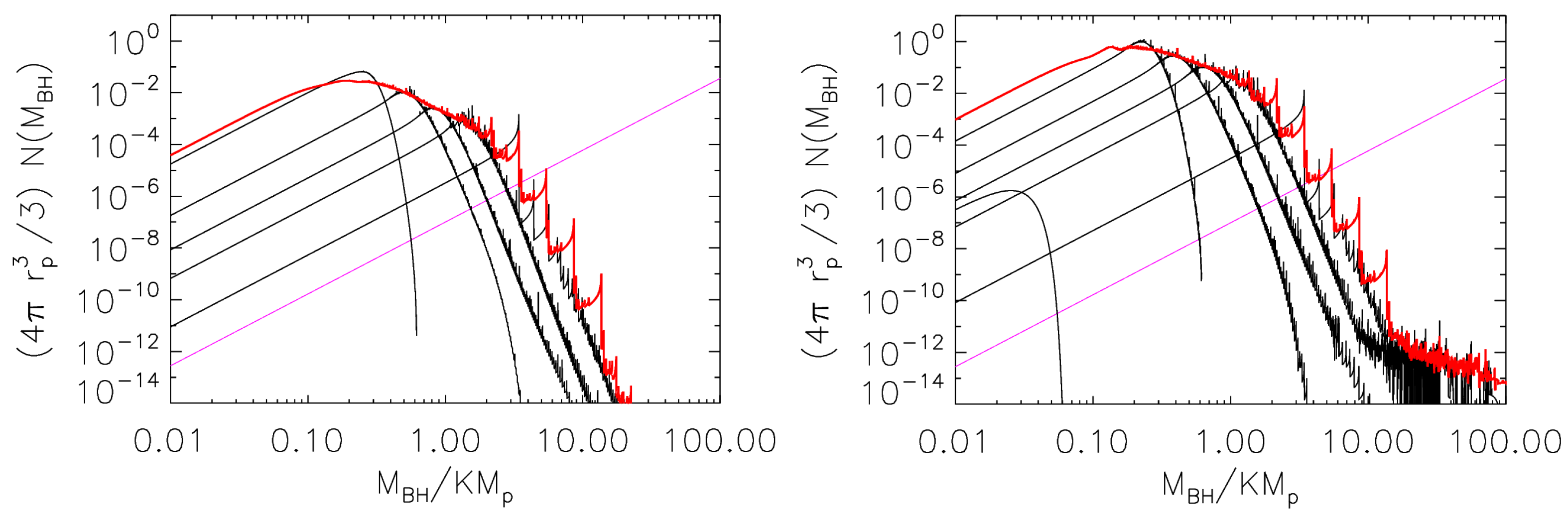
Figure 1 shows the dimensionless scaled mass function $\tilde{N}$ when $p=0$. The two panels show different values of $A_s$ for which ${\sigma }_0=0.33$ (left) and 0.6 (right). In each panel, the thick red curve shows $\tilde{N}\left(M_{•}\right)$; this is a power law at low masses (the magenta curve shows a power law of the expected slope, $1/0.36$) which is truncated exponentially at larger masses. Moreover, $\tilde{N}\left(M_{•}\right)$ is built up over time by summing over many ${\tilde{N}}_r\left(M_{•}\right)$; the solid curves show these for a few choices of r (with a larger r extending to larger $M_{•}$).

At any r, the shape of $N_r$ is a power law at low masses with an exponential truncation at larger masses. The amplitude of the power law part is clearly not monotonic in r, as neither a very small nor a very large r contributes to the final $N\left(M_{•}\right)$. Because r is related to the time of PBH formation, this explicitly shows that PBHs form over a range of times and that at any given time they can form with a wide spectrum of masses. Moreover, while there is a preferred formation time for $N_r$ as r changes, e.g., at the r for which the amplitude of the power law is greatest, the peak mass at this time is not the same as the peak mass of the red curve ($N\left(M_{•}\right)$). Thus, we cannot assume either a delta function in PBH formation times or an equivalent dominance of the mean profile for the compaction function.

Each $N_r\left(M_{•}\right)$ distribution, i.e., the mass function of black holes formed at a given time, is built from summing over different $N_{rw}\left(M_{•}\right)$ distributions, i.e., the mass function of black holes formed at a given time and with a given compaction function curvature. The thin curves of different styles in Figure 1 show $N_{rw}\left(M_{•}\right)$ for a few choices of r and w. The cutoff properties of $N_{rw}\left(M_{•}\right)$ can be understood as arising from the interplay between the pole in $d{g}_{•}/dln{M}_{•}$ (Equation (72)) and the exponential suppression from $p\left(g_{•}\right)$, with both acting to modify what would otherwise be a power law of slope $1/0.36=2.78$. In particular, here it can be seen explicitly that the exponential cutoff arises from the fact that for a given r and w there is a maximum possible mass which is set by requiring $g_{•}\le 4/3$; note that this is slightly more stringent than just saying that the mass cannot exceed that within the horizon. For a given $A_s$, this maximum is larger if r is larger and smaller if w is larger, which is because $C_c\left(w\right)$ increases as w increases. Finally, just as we cannot assume a delta function in r, we cannot assume a delta function in w either. This once again shows that the use of a mean profile would provide an incorrect result.

To illustrate how the shape rather than the amplitude of the power spectrum affects the predictions, Figure 2 shows a similar analysis of the case in which $p=2$. The mass spectrum clearly peaks at a lower $M_{•}/M_p$ than before, and the range of r that contributes significantly is smaller than before as well; however, the qualitative trends remain: a power law of slope $1/0.36$ at lower masses is truncated at larger masses, at first gradually and then exponentially.

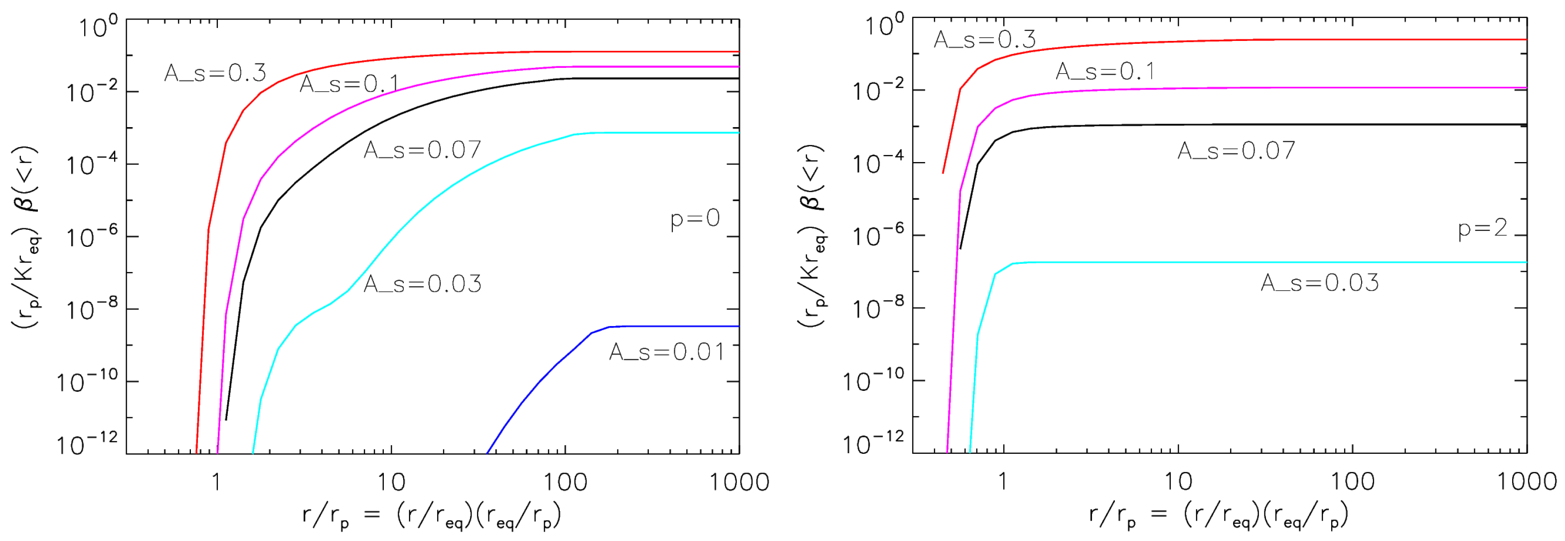
4.2.2. Dependence of the Abundance on the Power Spectrum

Figure 3 shows how the predicted abundance (Equation (64)) for a given maximal scale $r_{max}$ depends on $\mathcal{P}\left(k\right)$. The two panels are for two different $\mathcal{P}\left(k\right)$, and the different curves in each panel are for different amplitudes $A_s$. Because the horizontal axis is a proxy for the formation time, the flattening of the curves at $r\gg r_p$ is another indication that PBHs do not form at very late times. The steepness of these curves, i.e., how rapidly they rise to their asymptotic value, is a measure of the narrowness of the distribution of PBH formation times. Evidently, in the panel on the right this distribution is rather narrow, whereas in the panel on the left it is broader. In both panels, a smaller amplitude of $\mathcal{P}\left(k\right)$ results in a broader range of formation times.

As expected, it can be observed that the abundances related to very small power spectrum amplitudes are exponentially suppressed. This is due to the fact that essentially all variances decrease with $A_s$. Thus, for a very small power spectrum, in order to have ${\beta }_{•}\sim 1$ we would need $r_p$ to be much smaller than $r_{eq}$. On the contrary, a relatively large amplitude is related to a power spectrum peak position closer to the scale of matter–radiation equality.

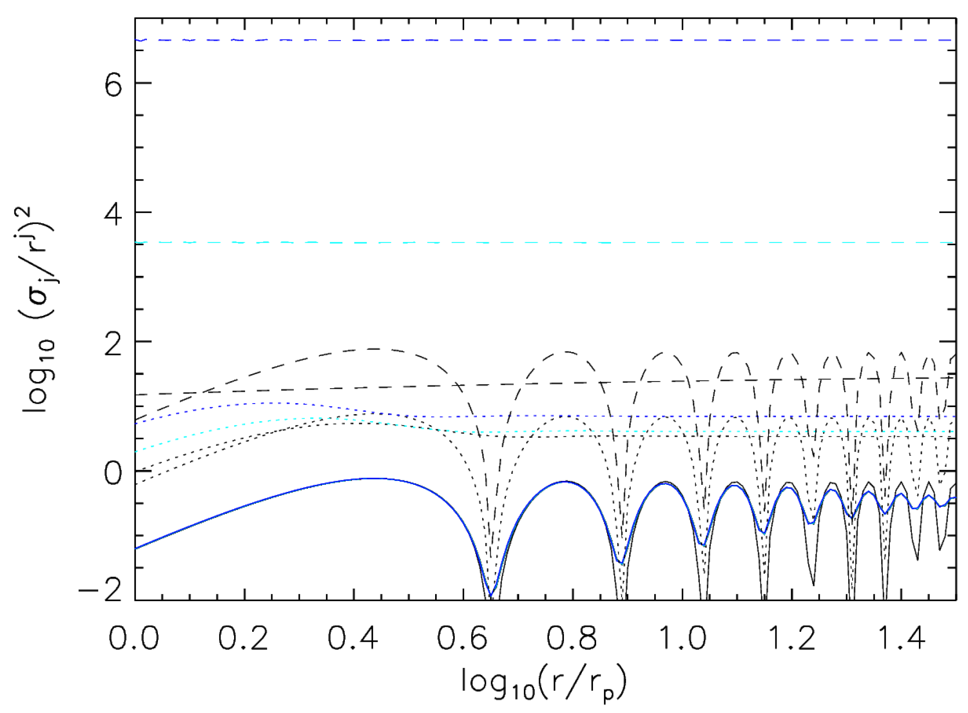
Finally, another power spectrum shape that has appeared in the literature is the log-normal one, which sets

$${\mathcal{P}}_{\mathrm{LN}}\left(k\right)=A_s{\mathrm{e}}^{-{[ln(k/k_p)]}^2/2{\sigma }_{\mathrm{LN}}^2}.$$

(88)

Here, ${\sigma }_{\mathrm{LN}}$ determines the width of the feature, which is centered on $k_p$. For small ${\sigma }_{\mathrm{LN}}$, ${\sigma }_j$ are not monotonic functions of r (see Figure 4); this can be understood by considering the delta function limit discussed in the sharp spectrum section and noting that $W\left(kr\right)$ oscillates (and strongly!). At larger r, the ${\sigma }_j$ in this model is asymptotic with respect to the ${\sigma }_j\propto r^j$ scaling noted earlier. In this respect, the model does not provide any new insights compared to what we have already studied in this section, and we do not consider it further.

5. Conclusions

In this paper, we have reviewed a framework for nonlinear estimation of the abundances of PBHs formed at times when radiation dominated the energy density of the universe. Our method explicitly differs from others in the literature in that it accounts for the fact that PBHs form at positions and scales where all possible statistical realizations of compaction functions (Equation (24)) are maximized. These positions and scales are intimately related to the formation time of black holes.

Apart from predicting the PBH abundance for any given inflationary power spectrum, we have studied their mass distribution, that is, the mass function. We show that the latter is generically a power law at low masses (Figure 1 and Figure 2). The slope of this power law depends on the critical scaling law for PBH formation (Equation (72)), and is independent of the shape or amplitude of the underlying power spectrum of fluctuations. At larger masses, there is a cutoff which depends on the shape and amplitude of the power spectrum (Figure 1 and Figure 2).

Our analysis shows that smaller amplitudes generically result in PBH formation that extends over a larger range in r (compare the top and bottom curves in left panel of Figure 3), i.e., over a longer range of times. In this regard, models which arbitrarily assume a single epoch of PBH formation related to a peak scale of the power spectrum ($r_p$) should be treated with skepticism. On the other hand, PBHs considerably lighter than $M_{\mathrm{eq}}$ (the mass of the cosmological horizon at matter–radiation equality) require $r_p\ll M_{\mathrm{eq}}^{-1}$ and a small $A_s$. Exactly how small depends on the shape of $\mathcal{P}\left(k\right)$, and is the subject of ongoing work. The fact that we can treat the whole of Dark Matter as being contained in PBHs, even with a small power spectrum, is related to the fact that the mass spectrum is broader when the amplitude of the power spectrum is smaller, as can be seen Figure 1 and Figure 2. As a byproduct, this cautions against analyses which assume that all PBHs have the same mass.

Finally, we would like to remark that all of our results in this paper depend critically on not including a transfer function when integrating over a power spectrum to compute our statistics. We have provided a detailed discussion of why a transfer function should not be used in our setup, in particular because of the way in which the compaction function is defined.

References

- Carr, B.; Kohri, K.; Sendouda, Y.; Yokoyama, J. Constraints on Primordial Black Holes. Rep. Prog. Phys. 2021, 84, 116902. [Google Scholar] [CrossRef] [PubMed]
- Escrivà, A. PBH Formation from Spherically Symmetric Hydrodynamical Perturbations: A Review. Universe 2022, 8, 66. [Google Scholar] [CrossRef]
- Thorne, K.S. Nonspherical Gravitational Collapse: A Short Review. In Magic without Magic; Klauder, J., Ed.; Freeman: San Francisco, CA, USA, 1972. [Google Scholar]
- Misner, C.W.; Sharp, D.H. Relativistic equations for adiabatic, spherically symmetric gravitational collapse. Phys. Rev. 1964, 136, B571–B576. [Google Scholar] [CrossRef]
- Shibata, M.; Sasaki, M. Black hole formation in the Friedmann universe: Formulation and computation in numerical relativity. Phys. Rev. D 1999, 60, 084002. [Google Scholar] [CrossRef]
- Musco, I. Threshold for Primordial Black Holes: Dependence on the shape of the cosmological perturbations. Phys. Rev. D 2019, 100, 123524. [Google Scholar] [CrossRef]
- Harada, T.; Yoo, C.M.; Koga, Y. Revisiting compaction functions. arXiv 2023, arXiv:2304.13284. [Google Scholar]
- Bardeen, J.M.; Bond, J.R.; Kaiser, N.; Szalay, A.S. The Statistics of Peaks of Gaussian Random Fields. Astrophys. J. 1986, 304, 15–61. [Google Scholar] [CrossRef]
- Escrivà, A. Simulation of primordial black hole formation using pseudo-spectral methods. Phys. Dark Univ. 2020, 27, 100466. [Google Scholar] [CrossRef]
- Cruces, D. Review on Stochastic Approach to Inflation. Universe 2022, 8, 334. [Google Scholar] [CrossRef]
- Cruces, D.; Germani, C. Stochastic inflation at all order in slow-roll parameters: Foundations. Phys. Rev. D 2022, 105, 023533. [Google Scholar] [CrossRef]
- Nadezhin, D.K.; Novikov, I.D.; Polnarev, A.G. The hydrodynamics of primordial black hole formation. Sov. Astron. 1978, 22, 129. [Google Scholar]
- Novikov, I.D.; Polnarev, A.G. The Hydrodynamics of Primordial Black Hole Formation-Dependence on the Equation of State. Sov. Astron. 1980, 24, 147. [Google Scholar]
- Polnarev, A.G.; Musco, I. Curvature profiles as initial conditions for primordial black hole formation. Class. Quant. Grav. 2007, 24, 1405–1432. [Google Scholar] [CrossRef]
- Harada, T.; Yoo, C.M.; Nakama, T.; Koga, Y. Cosmological long-wavelength solutions and primordial black hole formation. Phys. Rev. D 2015, 91, 084057. [Google Scholar] [CrossRef]
- Germani, C.; Musco, I. Abundance of Primordial Black Holes Depends on the Shape of the Inflationary Power Spectrum. Phys. Rev. Lett. 2019, 122, 141302. [Google Scholar] [CrossRef]
- Yoo, C.M.; Harada, T.; Garriga, J.; Kohri, K. Primordial black hole abundance from random Gaussian curvature perturbations and a local density threshold. PTEP 2018, 2018, 123E01. [Google Scholar] [CrossRef]
- Yoo, C.M.; Harada, T.; Hirano, S.; Kohri, K. Abundance of Primordial Black Holes in peak theory for an arbitrary power spectrum. PTEP 2021, 2021, 013E02. [Google Scholar] [CrossRef]
- Germani, C.; Sheth, R.K. Nonlinear statistics of Primordial Black Holes from Gaussian curvature perturbations. Phys. Rev. D 2020, 101, 063520. [Google Scholar] [CrossRef]
- Escrivà, A.; Germani, C.; Sheth, R.K. Universal threshold for primordial black hole formation. Phys. Rev. D 2020, 101, 044022. [Google Scholar] [CrossRef]
- Escrivà, A.; Germani, C.; Sheth, R.K. Analytical thresholds for black hole formation in general cosmological backgrounds. JCAP 2021, 2021, 030. [Google Scholar] [CrossRef]
- Musco, I.; Luca, V.D.; Franciolini, G.; Riotto, A. Threshold for Primordial Black Holes. II. A simple analytic prescription. Phys. Rev. D 2021, 103, 063538. [Google Scholar] [CrossRef]
- Akrami, Y.; Arroja, F.; Ashdown, M.; Aumont, J.; Baccigalupi, C.; Ballardini, M.; Banday, A.J.; Barreiro, R.B.; Bartolo, N.; Basak, S.; et al. Planck 2018 results. IX. Constraints on primordial non-Gaussianity. Astron. Astrophys. 2020, 641, A9. [Google Scholar]
- Germani, C.; Prokopec, T. On Primordial Black Holes from an inflection point. Phys. Dark Univ. 2017, 18, 6–10. [Google Scholar] [CrossRef]
- Motohashi, H.; Hu, W. Primordial Black Holes and Slow-Roll Violation. Phys. Rev. D 2017, 96, 063503. [Google Scholar] [CrossRef]
- Özsoy, O.; Tasinato, G. Inflation and Primordial Black Holes. Universe 2023, 9, 203. [Google Scholar] [CrossRef]
- Atal, V.; Germani, C. The role of non-gaussianities in Primordial Black Hole formation. Phys. Dark Univ. 2019, 24, 100275. [Google Scholar] [CrossRef]
- Atal, V.; Garriga, J.; Marcos-Caballero, A. Primordial black hole formation with non-Gaussian curvature perturbations. JCAP 2019, 2019, 073. [Google Scholar] [CrossRef]
- Pi, S.; Sasaki, M. Logarithmic Duality of the Curvature Perturbation. Phys. Rev. Lett. 2023, 131, 011002. [Google Scholar] [CrossRef]
- Press, W.H.; Schechter, P. Formation of galaxies and clusters of galaxies by selfsimilar gravitational condensation. Astrophys. J. 1974, 187, 425–438. [Google Scholar] [CrossRef]
- Bond, J.R.; Cole, S.; Efstathiou, G.; Kaiser, N. Excursion set mass functions for hierarchical Gaussian fluctuations. Astrophys. J. 1991, 379, 440. [Google Scholar] [CrossRef]
- Sheth, R.K. Symmetry in stochasticity: Random walk models of large scale structure. Pramana-J. Phys. 2011, 77, 169–184. [Google Scholar] [CrossRef]
- Paranjape, A.; Sheth, R.K. Peaks theory and the excursion set approach. MNRAS 2012, 426, 2789–2796. [Google Scholar] [CrossRef]
- Paranjape, A.; Sheth, R.K.; Desjacques, V. Excursion Set Peaks: A self-consistent model of dark halo abundances. MNRAS 2013, 431, 1503–1512. [Google Scholar] [CrossRef]
- Kalaja, A.; Bellomo, N.; Bartolo, N.; Bertacca, D.; Matarrese, S.; Musco, I.; Raccanelli, A.; Verde, L. From Primordial Black Holes Abundance to Primordial Curvature Power Spectrum (and back). JCAP 2019, 10, 031. [Google Scholar] [CrossRef]
- Luca, V.D.; Kehagias, A.; Riotto, A. How Well Do We Know the Primordial Black Hole Abundance? The Crucial Role of Non-Linearities when Approaching the Horizon. arXiv 2023, arXiv:2307.13633. [Google Scholar]
- Kopp, M.; Hofmann, S.; Weller, J. Separate Universes Do Not Constrain Primordial Black Hole Formation. Phys. Rev. D 2011, 83, 124025. [Google Scholar] [CrossRef]
- Harada, T.; Carr, B.J.; Igata, T. Complete conformal classification of the Friedmann–Lemaître–Robertson–Walker solutions with a linear equation of state. Class. Quantum Grav. 2018, 35, 105011. [Google Scholar] [CrossRef]
- Niemeyer, J.C.; Jedamzik, K. Dynamics of Primordial Black Hole Formation. Phys. Rev. D 1999, 59, 124013. [Google Scholar] [CrossRef]
- Escrivà, A.; Romano, A.E. Effects of the shape of curvature peaks on the size of Primordial Black Holes. JCAP 2021, 05, 066. [Google Scholar] [CrossRef]
- Escrivà, A.; Atal, V.; Garriga, J. Formation of trapped vacuum bubbles during inflation, and consequences for PBH scenarios. arXiv 2023, arXiv:2306.09990. [Google Scholar]
- Yokoyama, J. Cosmological constraints on Primordial Black Holes produced in the near-critical gravitational collapse. Phys. Rev. D 1998, 58, 107502. [Google Scholar] [CrossRef]
- Özsoy, O.; Tasinato, G. On the slope of the curvature power spectrum in non-attractor inflation. JCAP 2020, 04, 048. [Google Scholar] [CrossRef]
- Cole, P.S.; Gow, A.D.; Byrnes, C.T.; Patil, S.P. Steepest growth re-examined: Repercussions for primordial black hole formation. arXiv 2023, arXiv:2204.07573. [Google Scholar]
Figure 1.
Distribution of when has slope and amplitude such that (left) and (right). The thick red curve in each panel shows the scaled mass function (Equation (87)), which results from summing over distributions, a selection of which are shown as thick black curves (with a larger r extending to larger ). Each of these results from summing over different (cf. Equation (74)), which we show for a few representative values of w (dotted, short-dashed, dot-dashed, dot-dot-dot-dashed, long dashed). At small r, increasing w decreases the maximum mass, while at larger r the mass function is a power law with a small divergence at the largest allowed masses; the amplitude of this power law depends on w and qualitatively traces the distribution of w, i.e., it is small at both small and large values of w. The magenta line shows a power law of slope , which we argue in the text to be a good approximation at small .
Figure 2.
Same as in the previous figure, except now with having a slope and without any curves. The right-hand panel has , while the left hand panel has the same as in Figure 1; however, the value of is similar to that in the right hand panel of Figure 1. For the same , the mass spectrum peaks at smaller compared to , while the power law slope at low masses (magenta) is the same.
Figure 3.
Dependence of scaled mass fraction at equality (Equation (86)), that is, in PBHs which formed before r; the panels show results for having (left) and (right); the different curves in each panel are for different amplitudes (as labeled). In both cases, this quantity is smaller if is smaller. For , most PBHs form when r is slightly smaller than ; for the range of is broader, especially for small amplitudes.
Figure 4.
Value of in the Log-normal model for (solid), (dotted), and 3 (dashed) for (black), (cyan), and (blue) with . Curves which drop to zero show the delta function limit () of . Larger are simply smeared versions of this limit, and at large , is constant.
Disclaimer/Publisher’s Note: The statements, opinions and data contained in all publications are solely those of the individual author(s) and contributor(s) and not of MDPI and/or the editor(s). MDPI and/or the editor(s) disclaim responsibility for any injury to people or property resulting from any ideas, methods, instructions or products referred to in the content. |
© 2023 by the authors. Licensee MDPI, Basel, Switzerland. This article is an open access article distributed under the terms and conditions of the Creative Commons Attribution (CC BY) license (https://creativecommons.org/licenses/by/4.0/).
Share and Cite
MDPI and ACS Style
Germani, C.; Sheth, R.K. The Statistics of Primordial Black Holes in a Radiation-Dominated Universe: Recent and New Results. Universe 2023, 9, 421. https://doi.org/10.3390/universe9090421
AMA Style
Germani C, Sheth RK. The Statistics of Primordial Black Holes in a Radiation-Dominated Universe: Recent and New Results. Universe. 2023; 9(9):421. https://doi.org/10.3390/universe9090421
Chicago/Turabian StyleGermani, Cristiano, and Ravi K. Sheth. 2023. "The Statistics of Primordial Black Holes in a Radiation-Dominated Universe: Recent and New Results" Universe 9, no. 9: 421. https://doi.org/10.3390/universe9090421
Note that from the first issue of 2016, this journal uses article numbers instead of page numbers. See further details here.