Spectral Line Shapes of He I Line 3889 Å

Abstract

Spectral line shapes of neutral helium 3889 Å ($2^{3}S$–$3^{3}P$) transition line are calculated by using several theoretical methods. The electronic contribution to the line broadening is calculated from quantum statistical many-particle theory by using thermodynamic Green’s function, including dynamic screening of the electron-atom interaction. The ionic contribution is taken into account in a quasistatic approximation, where a static microfield distribution function is presented. Strong electron collisions are consistently considered with an effective two-particle T-matrix approach, where Convergent Close Coupling method gives scattering amplitudes including Debye screening for neutral helium. Then the static profiles converted to dynamic profiles by using the Frequency Fluctuation Model. Furthermore, Molecular Dynamics simulations for interacting and independent particles are used where the dynamic sequence of microfield is taken into account. Plasma parameters are diagnosed and good agreements are shown by comparing our theoretical results with the recent experimental result of Jovićević et al. (J. Phys. B: At. Mol. Opt. Phys. 2005, 38, 1249). Additionally, comparison with various experimental data in a wide range of electron density $n_e\approx ({10}^{22}-{10}^{24}){\mathrm{m}}^{-3}$ and temperature $T\approx (2-6)\times {10}^4$ K are presented.

1. Introduction

Calculation of spectral line shapes is a most powerful tool for plasma diagnostic in both the star atmosphere and in laboratory plasmas. Perturbation of the radiating atom or ion by the surrounding particles leads to spectral line broadening (Stark broadening), while the coherent emission process is interrupted by collisions and influenced by plasma microfield. Several theoretical approaches have been applied to calculate Stark broadening, such as the well known semiclassical approximation the standard theory (ST) by Griem [1], or the quantum statistical approach of many-particle theory [2], where the motion of ion perturber is neglected during the inverse halfwidth of the line. Furthermore, the model microfield method (MMM) [3,4,5,6], the frequency fluctuation method (FFM) [7] or computer simulations [8,9,10,11] are used for calculating the line broadening including ion-dynamics effects, which lead to further broadening of the line shapes.

In this work, we describe several theoretical approaches to study the He I 3889Å ($2^{3}S$–$3^{3}P$) transition line. Plasma parameters are determined by comparing our theoretical results with the measurement of Jovićević et al. [12]. In our quantum statistical approach, thermodynamic Green’s function is used for calculating emitted or absorbed radiation from bound–bound transition of charge particles by using two-particle polarization function [13,14,15,16], which is related to the Fourier transformation of the imaginary part of the dipole–dipole correlation function. In principle, this approach is able to describe the dynamic screening and strong collision by electrons in a systematic way. The quantum statistical approach can adequately treat electron collisions. To obtain full profiles, it has been supplemented by a calculation of ion broadening done by other methods and thereby has been successfully applied to calculate the line profile of hydrogen and H-like ions [17]. The strong collisions of an electron-emitter pair are treated within a T-matrix approach by solving close-coupling equations to produce forward scattering amplitudes. Ions are treated in a quasistatic approximation via the microfield distribution function. Then the latest formulation of the FFM is applied to account for ion dynamics [18]. On the other hand, computer simulations accounting simultaneously for the electronic and ionic fields on the same footing are used for comparison. Recently, the shift and width of this line was computed by Lorenzen et al. [19], comparison was made with various theoretical and measurement data in a wide range of electron density and temperature. In Section 2 we describe briefly the experimental setup and result of Jovićević et al. [12]. Our theoretical approaches for calculating the line shapes are reviewed in Section 3, followed by results and discussions Section 4.

2. Experiment

In this paper, we analyze theoretically the He I 3889 Å Stark broadening, measured by Jovićević et al. [12] from a pulsed low-pressure capillary discharge. The plasma was a mixture of neon, helium and hydrogen, with the predominant H${}^{+}$ perturber ions. Originally the experiment was set up for the measurement of Ne I spectral line profiles, while He was added to the gas mixture for plasma diagnostic purpose. The presence of hydrogen increases the electron density to the required value until a constant value of the Stark width was recorded. The optimum gas mixture was determined in a series of measurements starting from pure neon and then diluting until optically thin Ne I lines were recorded. In the experiment, a quartz discharge tube with 3 mm inner diameter and length of $7.2$ cm was used, and aluminum electrodes with 3 mm diameter holes were located 200 mm apart. The measurements were performed in a premixed gas mixture of $2.4\%$ Ne, $5.6\%$ He and $92\%$ H${}_2$ by volume, at an initial pressure of 4 mbar. Spectroscopic plasma observations of Ne I and He I lines were performed, measuring the line shapes at the same time of plasma decay. The dilution of neon and helium with hydrogen was done in order to increase the electron density, since H has much lower ionization potential than Ne and He, and to generate a plasma with H${}^{+}$ ions dominating He${}^{+}$ and Ne${}^{+}$. Special care was taken to keep the line profiles optically thin during measurements, in order to minimize self-absorption. This was achieved by using a continuous gas flow and diluting neon with helium and hydrogen in the operated arc. Moreover, plasma radiation was observed from the axial narrow discharge tube as well as from the radial expanded part simultaneously. However, the experimental design and procedure may have resulted in plasma inhomogeneity which may cause line distortion and line asymmetry. Electron density was determined from the measured He I line profiles, which were assumed to be optically thin under the same plasma conditions. The experimental profiles were fitted to a semiclassical calculation using two parameters, the electron impact width and the ion-broadening parameter A of the quasistatic approximation [1], which allow the authors to determine the electron density. The mean value of electron density $n_e$ was estimated to be $4.8\times {10}^{22}{\mathrm{m}}^{-3}$ with an estimated uncertainty of $\pm 10\%$. By assuming local thermal equilibrium, the electron temperature $T_e=T_i=3.3\times {10}^4$ K was determined from the Boltzmann plot of O II impurity lines with an uncertainty of ±$12\%$, as the Stark broadening parameters weakly depend upon $T_e$. More details about the experimental set up and measurement are given in [12].

3. Theoretical Approaches

In this section we present the different kinds of theoretical approaches that we used for calculating He I line profiles.

3.1. Quantum Statistical Approach

In quantum statistical many-particle theory, the medium effects are taken into account by using the thermodynamic Green’s function technique to describe the Stark broadening. The perturbing electrons and ions can be treated independently due to variety of mass between them ($m_e<<m_i$). The dynamically screened Born approximation applied for electron-emitter interaction, while almost stationary heavy ions are treated in a quasistatic ion approximation due to static microfield. Spectral line broadening is given by the imaginary part of the second order two-particle polarization function, which is a bound–bound transition. The polarization function is calculated in a systematic way from thermodynamic Green’s functions and is proportional to the Fourier transform of the dipole–dipole autocorrelation function (see Appendix A). The perturber–radiator interaction leads to the pressure broadening, including both the electronic and the ionic contributions in the quasistatic limit by averaging the static microfield distribution function $W(\beta )$ [14,15,16], and we get

$$\begin{array}{cc}\hfill I^{\mathrm{pr}}(\omega ) \hspace{1em}\sim & \sum _{i^{\prime },i^{″},f^{\prime },f^{″}}\langle i^{\prime }\left|\mathbf{r}\right|f^{\prime }\rangle \langle f^{{}^{″}}\left|\mathbf{r}\right|i^{{}^{″}}\rangle \frac{{\omega }^4}{8{\pi }^3{c}^3}{\mathrm{e}}^{-\frac{\hslash \omega }{k_{\mathrm{B}}T}}{\int }_0^{\infty }W(\beta )d\beta \hfill \\ & \times \mathrm{Im}\langle i^{\prime }|\langle f^{\prime }|{\left[\hslash \omega -\hslash {\omega }_{if}-{\Sigma }_{if}(\omega ,\beta )+ı{\Gamma }_{if}^{\mathrm{v}}\right]}^{-1}|f^{{}^{″}}\rangle |i^{{}^{″}}\rangle \hfill \end{array}$$

(1)

where $\langle i\left|\mathbf{r}\right|f\rangle$ is identified as a dipole matrix-element for the transition probability between initial $(n_i,l_i,m_i)$ and final $(n_f,l_f,m_f)$ states. The ionic microfield strength $\beta =E/E_0$ is normalized to the Holtsmark field $E_0$, and $\hslash {\omega }_{if}=E_i-E_f$ is the unperturbed transition energy. The interference correction ${\Gamma }_{if}^{\mathrm{v}}$ for the overlapping line is related to coupling between the initial and final states, the interference contribution vanishes for this transition because the lower state is a s-state and thus not collisionally connected to itself.

The interference term is less important for neutral helium, and is ignored in the dipole approximation, this is not the case for quadrupole approximation of transition [1,20]. However, more accurate calculations are needed for lines involving transitions with high excited states, which are almost hydrogenic states of the helium atom. If the contribution of the lower levels is neglected, then the interference term is zero [21]. Generally the interference contribution is less important for non-hydrogenic line transitions [20]. The function ${\Sigma }_{if}(\omega ,\beta )$ is determined by the self-energy correction ${\Sigma }_n(\omega ,\beta )$ of the initial and the final states

$${\Sigma }_{if}(\omega ,\beta )=\mathrm{Re}\left[{\Sigma }_i(\omega ,\beta )-{\Sigma }_f(\omega ,\beta )\right]+ı\mathrm{Im}\left[{\Sigma }_i(\omega ,\beta )+{\Sigma }_f(\omega ,\beta )\right]$$

(2)

where the real part represents the shift ${\Delta }_n^{\mathrm{SE}}$ and the imaginary part gives the width ${\Gamma }_n^{\mathrm{SE}}$ of each state. The electronic and ionic contributions occur in the self-energy. Performing Born approximation with respect to the dynamically screened perturber–radiator potential $V(q)$, the diagonal elements of electronic self-energy operator is obtained as (see Appendix B)

$$\begin{array}{ccc}\hfill {\Delta }_n^{\mathrm{SE}}+ı{\Gamma }_n^{\mathrm{SE}}& =& <n|{\displaystyle {\Sigma }^{\mathrm{el}}(E_n,\beta )|n>=-\frac{1}{e^2}\int \frac{{\mathrm{d}}^{3}q}{{(2\pi )}^3}V(q)\sum _{\alpha }{\left|M_{n\alpha }(\mathbf{q})\right|}^2}\hfill \\ & & \times \underset{-\infty }{\overset{\infty }{\int }}\frac{\mathrm{d}\omega }{\pi }[1+n_{\mathrm{B}}(\omega )]\frac{\mathrm{Im}{\epsilon }^{-1}(\mathbf{q},\omega +ı0)}{E_n-E_{\alpha }(\beta )-\hslash (\omega +ı0)}.\hfill \end{array}$$

(3)

Here, the level splitting ($E_{\alpha }(\beta )\approx E_{\alpha }$) due to the microfield has been neglected, $n_{\mathrm{B}}(\omega )={\left[exp(\hslash \omega /k_{\mathrm{B}}T)-1\right]}^{-1}$ is the Bose distribution function, approximated by the Boltzmann distribution function for non-degenerated plasma. The sum over principal quantum number α runs from $n-2$ to $n+2$ discrete bound states for the virtual transitions. Dynamic screening is obtained from the imaginary part of the inverse dielectric function ${\epsilon }^{-1}(\mathbf{q},\omega )$, for which the random phase approximation (RPA) is used. The transition matrix-element $M_{n\alpha }(\mathbf{q})$ describes the interaction of the atom with the Coulomb potential through the vertex function, where the Coulomb interaction with the electron-electron-ion triplet depends on the momentum transfer $\hslash \mathbf{q}$ (see Appendix C). The electron wavefunctions for helium are obtained by applying the Coulomb approximation method [22]. In the Born approximation, the electronic contribution is overestimated. Hence, in order to avoid this, we apply the cut-off procedure and add the strong collisions term [1,16,23] instead of the partial summation via the T-matrix. For He I we adopt the cut-off parameter and close electron-radiator collisions term, evaluated according to the semiclassical estimation, see [16,23]. For non-hydrogenic radiator the ionic contribution to the self-energy is related to the quadratic Stark effect and quadrupole interaction [24], further details are given in [15,16].

The above procedure is used to describe the perturbing effect of free electrons on the radiator from the electronic self energy and the interference correction, which gives exactly the same expression as the semiclassical impact approximation of Griem [1], if the term with $q^2$ is neglected in the argument of delta function as in the classical limit, see Equation (4.5) in [13]. The comparison between the Green’s function approach and impact approximation is proved in detail by Kraeft et al. [25].

3.1.1. T-Matrix Approach

The electronic contribution can be evaluated again from the effective T-matrix approach which is based on the partial summation. To avoid the cut-off procedure for strong electron-atom collisions, the electronic contribution to shift and width of spectral lines can be treated via partial summation of the three-particle T-matrix. A three-particle propagator ($T_3$) in the channel of the two-particle bound state and perturbing electron was adopted by Günter [2,26] for calculating the hydrogen L${}_{\alpha }$ line. It can describe weak and strong collisions within static Debye screening. For a non-degenerate plasma, the electronic contribution can be evaluated from scattering amplitudes, characterized by the self energy [19]

$${\Sigma }_n^{\mathrm{el}}=-\frac{2}{\pi }{n}_e{\Lambda }_{\mathrm{th}}^3{\int }_0^{\infty }dk{k}^2{e}^{-k^2/(k_{\mathrm{B}}T)}{f}_n(0,k).$$

(4)

Here, ${\Lambda }_{\mathrm{th}}=\sqrt{4\pi /(k_{\mathrm{B}}T)}$ is thermal wave length, and $f_n(\theta =0,k)$ are forward scattering amplitudes of elastic electron scattering at the Debye screened He I for both state initial $(n=i)$ and final $(n=f)$ states, respectively. The singlet $S=0$ and triplet $S=1$ channels for scattering are considered for both initial i and final f states. This expression was also found by Baranger [27]. The single electron-atom and -ion scattering problem is studied to provide reliable results for all transitions of interest including elastic, excitation, ionization, and total cross sections [28,29,30]. Recently, the electron-helium scattering in weakly coupled hot-dense plasmas has been investigated by using the Convergent Close Coupling method (CCC), where the Laguerre basis expansions are applied to obtain fully convergent scattering amplitudes in the close-coupling equations. The screened Coulomb potential or Debye-Hückel potential [31,32] has been employed. This Yukawa-type potential has been used to describe the plasma Coulomb screening effect by formulating a set of close-coupling equations for the T-matrix approach by providing a complete description of the scattering process. The CCC method solves the close-coupling equations in momentum space and uses the T-matrix to determine the cross sections and forward scattering amplitudes for dipole and spin-allowed transitions on the Debye screened neutral helium atom, The CCC method uses the analytical Born subtraction technique to speed up the convergence of the partial-wave expansion, thus the first Born approximation matrix elements for inelastic scattering is modified. The quantum system involves electron-helium scattering from the ground-state state up to 4f with the correct energies using 153 pseudo-states to describe the scattering, more details are given in [33,34,35]. Our method gives different results for singlet and triplet scattering channels as well as for scattering at the emitter with initial and final states. Here, we consider only the electron-He forward elastic scattering amplitudes $f(0,k)$ from initial state $(n_i,l_i,m_i)$ to final state $(n_f,l_f,m_f)$ for the self-energies, where $n,l,m$ are the well known principal quantum numbers. Here, the transitions $2S\to 2S$ and $3P\to 3P$ are considered for double channel transitions. For a detailed description of the T-matrix calculation see [19].

3.1.2. Microfield Distribution Function

The ionic microfield is considered to be constant during the time of interest of the order of the inverse HWHM of the line, so that a static description of the microfield can be used. In this study, the plasma microfield distribution function is calculated by taking into account the screening and quantum effects of diffraction, the evaluated distribution function is used for calculating line broadening for analyzing the experimental data of Jovićević et al. [12]. Processes such as ionization, dissociation, and excitation of bound states occur continuously in plasma and affect plasma properties and its compositions [36]. The distribution of charged particles in the system within the Debye radius $r_D$ is not homogeneous at distances $r<r_D$, although the plasma is electrically neutral as a whole, but at sufficiently small distances the fluctuation of the local electric field affects the plasma kinetic coefficients, optical and thermodynamic properties, etc. [37]. According to Ecker and Müller [38] the effective Debye screened field is defined as

$$\overrightarrow{E}=\frac{e}{r^3}\overrightarrow{r}(1+r/r_D)e^{-r/r_D}$$

(5)

The problem of microfield distribution is formally similar to the problem of determining the chemical potential. This allowed Iglesias [39] to reduce the microfield problem to finding the radial distribution functions (RDF) of some fictitious system with a complex potential energy of interaction. This made the basis for the development of the integral equations method to study the problem of the plasma microfield distribution.

In this paper, we use a method for calculating the distribution function of ionic microfield component $P(E)$ proposed by Iglesias [40]. The advantage of this method is that the distribution function is exactly expressed in terms of a two-body function and does not require knowledge of many-body functions. We use a strongly coupled one component plasmas (OCP) model, i.e., in a fully ionized plasma, in which the electron component forms a homogeneous neutralizing background with N positively charged particles. The microfield distribution function $W(\overrightarrow{E})$ is defined as the probability of finding an electric field $\overrightarrow{E}$ at a charged point located at ${\overrightarrow{r}}_0$. It is generally expressed in terms of the probability density $P_{N+1}({\overrightarrow{r}}_0,{\overrightarrow{r}}_1,...,{\overrightarrow{r}}_N)$ of finding a particular configuration of $(N+1)$ particles:

$$W(\overrightarrow{E})=\int ...\int \delta (\overrightarrow{E}-\sum _{j=1}^N\overrightarrow{E_j})P_{N+1}({\overrightarrow{r}}_0,{\overrightarrow{r}}_1,...,{\overrightarrow{r}}_N)d{\overrightarrow{r}}_0,d{\overrightarrow{r}}_1,...,d{\overrightarrow{r}}_N$$

(6)

where ${\overrightarrow{E}}_j$ is the electric field, created by $j-$th particle on radiating atoms or ions at ${\overrightarrow{r}}_0$. Assuming the system is isotropic we may introduce Fourier transformation of the function $W(\overrightarrow{E})$

$$\begin{array}{c}\hfill P(E)=\frac{2E}{\pi }{\int }_0^{\infty }lT(l)sin(El)dl\end{array}$$

(7)

where $T(l)$ is the characteristic function with a total pair correlation function $h(\overrightarrow{r};\lambda )$

$$lnT(l)=n{\int }_0^{1}d\lambda {\int }_0^{\infty }d\overrightarrow{r}\frac{ıq\widehat{l}\overrightarrow{r}}{r^3}h(\overrightarrow{r};\lambda )$$

(8)

with $\widehat{l}$ is a unit vector in the direction of $\overrightarrow{l}$, and the introduced parameter λ is a magnitude of the vector $\overrightarrow{l}$, while q is the charge of ions, immersed in a neutralizing electron background. The next step is a definition of $h(\overrightarrow{r};\lambda )$. The simplest approximation suitable for a Coulomb system is the Debye–Hückel theory. In this approximation we have

$$h(\overrightarrow{r};\lambda )\approx exp\{-\overline{\beta }[1-\frac{ı\lambda \overrightarrow{l}}{q\overline{\beta }}{\overrightarrow{\nabla }}_0]\Phi (r)\}-1.$$

(9)

In [41] with the help of linear response method an effective potential was obtained, which is also used in this paper, by taking in to account both the diffraction effects at short distances and the screening effect at large distances

$${\Phi }_{}(r)=-\frac{Z_{\alpha }{e}^2}{\sqrt{1-4{\lambda }_{\alpha e}^2/r_D^2}}\left(\frac{e^{-Br}}{r}-\frac{e^{-Ar}}{r}\right)$$

(10)

where

$$\begin{array}{ccc}\hfill A^2& =& \frac{1}{2\lambda }\left(1+\sqrt{1-4{\lambda }_{\alpha e}^2/r_D^2}\right)\hfill \end{array}$$

$$\begin{array}{ccc}\hfill B^2& =& \frac{1}{2\lambda }\left(1-\sqrt{1-4{\lambda }_{\alpha e}^2/r_D^2}\right).\hfill \end{array}$$

The coupling parameter is defined by $\Gamma =\overline{\beta }{e}^2/r_0$, and

$$r_D={(4\pi n{e}^2\overline{\beta })}^{1/2},\overline{\beta }={(k_{\mathrm{B}}T)}^{-1},r_0={(4\pi n/3)}^{-1/3}$$

(11)

where $r_0$ is the mean particle distance. Here the reduced form of pseudopotential is used

$$-\overline{\beta }\Phi (r)=-\frac{\Gamma }{R}\frac{1}{\sqrt{1-24{\Gamma }^2/(\pi r_s)}}\left(e^{-BR}-e^{-AR}\right)$$

(12)

with

$$\begin{array}{ccc}\hfill A^2& =& \frac{\pi r_s}{4\Gamma }\left(1+\sqrt{1-24{\Gamma }^2/(\pi r_s)}\right)\hfill \end{array}$$

$$\begin{array}{ccc}\hfill B^2& =& \frac{\pi r_s}{4\Gamma }\left(1+\sqrt{1-24{\Gamma }^2/(\pi r_s)}\right).\hfill \end{array}$$

In order to solve Equation (6) numerically, it is better to use the dimensionless field units and to introduce $l^{*}=E_{0}l$. Thus we obtain a formula to calculate the distribution of electric field $E^{*}$:

$$\mathcal{P}(E^{*})=\frac{2E^{*}}{\pi }{\int }_0^{\infty }d{l}^{*}lT(l^{*})sin(E^{*}{l}^{*}).$$

(13)

By substitution of Equation (9) into Equation (8) yields

$$\begin{array}{ccc}\hfill lnT(l)& =& 3{\int }_0^{\infty }dR·exp\left\{\frac{\Gamma }{R}\frac{1}{\sqrt{1-\chi }}(e^{-AR}-e^{-BR})\right\}\hfill \\ & & \times \frac{R^2}{e^{-BR}(1+BR)-e^{AR}(1+AR)}\hfill \end{array}$$

(14)

where $\chi =6{\Gamma }^2/(\pi r_s)$, $R=r/r_0$ and

$$lb(R)=\frac{lq}{r_0}\frac{e^{-BR}(1+BR)-e^{-AR}(1+AR)}{R^2}$$

The one-dimensional integration over R involves the sin transformation in Equation (7), in which $T(l)$ is defined by Equation (8) which is solved numerically.

The microfield distribution function illustrated here is applied for calculating the line profiles to determine the plasma parameters of the measured data by Jovićević et al. [12].

3.1.3. Frequency Fluctuation Model

Recently, Calisti et al. [18] presented a very fast method to account for ion dynamic effects on atomic spectra in plasmas. This method is based on reformulation for the frequency fluctuation model (FFM), which provides an expression of the dynamic line shapes based on a mixing frequency and the quasistatic Stark profiles. This method allows a very fast and accurate calculation of Stark broadening $I(\omega )$ by taking into account ion-dynamics in this expression

$$I(\omega )\sim \mathrm{Re}\frac{\int \frac{\mathcal{A}({\omega }^{\prime })d{\omega }^{\prime }}{\gamma +i(\omega -{\omega }^{\prime })}}{1-\gamma \int \frac{\mathcal{A}({\omega }^{\prime })d{\omega }^{\prime })}{\gamma +i(\omega -{\omega }^{\prime })}}.$$

(15)

Here, $\mathcal{A}(\omega )$ is the area-normalized line profile in quasistatic limit, evaluated from Equation (1), the inverse state lifetime $\gamma =v_{\mathrm{th}}/d$ is defined by ion thermal velocity of perturbers $v_{\mathrm{th}}=\sqrt{8k_{\mathrm{B}}T/(\pi m_i)}$ and the mean distance between ions $d={(4\pi n_i/3)}^{-1/3}$, where $m_i$ and $n_i$ are the mass and density of perturbing ions, respectively.

3.2. Classical Molecular Dynamics Simulations

Spectral line shapes $I(\Delta \omega )$ are also calculated using molecular dynamics (MD) simulations. Using these simulations, the dynamics of the particles in the plasma is reproduced numerically in the computer and the electric field sequences suffered by the emitters are obtained. These field sequences are taken to the differential equations that permit to calculate the emitter evolution, and the final profiles are obtained as the Fourier transform of an average of the emitter dipole-moment autocorrelation function [42].

$$\begin{array}{ccc}\hfill I(\Delta \omega )& =& \mathrm{Re}\frac{1}{\pi }{\int }_0^{\infty }dt\{C(t)\}{e}^{ı\Delta \omega t}\hfill \end{array}$$

(16)

$$\begin{array}{ccc}\hfill C(t)& =& \mathrm{tr}[\mathbf{D}(t)·\mathbf{D}(\mathbf{0})\rho ]\hfill \end{array}$$

(17)

$$\begin{array}{ccc}\hfill D(t)& =& U^{+}(t)\mathbf{D}(0)U(t)\hfill \end{array}$$

(18)

where ρ is the equilibrium density-matrix operator, D is the dipole operator for the radiating system, and the symbols $\{\}$ mean an average over a large number of simulated individual processes obtained in order to have a representative sampling of the electric fields in the plasma. $U(t)$ is the emitter time evolution operator that obeys Schrödinger equation

$$ı\hslash \frac{d}{dt}U(t)=H(t)U(t)=\left(H_0+q\mathbf{E}(t)·\mathbf{R}\right)U(t)$$

(19)

where the Hamiltonian $H(t)$ includes the structure of the emitter states without perturbation $H_0$, and the action of the perturbers through the dipole interaction with the electric field $\mathbf{E}(t)$ at the emitter location [43]. For a specific line transition, two groups of states are considered, the upper and lower group of states of the transition. If the difference in energy of those groups is large enough in comparison with the average energy of the collisions in the plasma, then we can assume that both groups of states evolve independently though undergoing the same sequence of perturbing electric field, which is known as the no-quenching approximation. The simulations used in this work consider that the perturbers are classical point independent particles that move along straight line trajectories with constant speeds according to the Maxwell distribution corresponding to their equilibrium temperature. Correlation effects between perturbers are taken into account considering Debye screened electric fields. The relative movement of the heavy perturbers and the emitter is taken into account using the reduced mass of the emitter-perturber pair according to the μ-ion model [44]. This simulation technique is designed to guarantee that the density of particles within the simulation sphere is kept constant along the simulation and that both the spatial distribution of particles and the velocities distribution are kept stationary [9]. On the other hand, this technique allows us to consider non-equilibrium plasmas [45], and can also be applied to non-homogeneous plasmas [46,47]. However, for strongly interacting plasmas (large plasma coupling parameter) or charged emitters, MD simulations accounting for the interactions between all the particles in the plasma (i.e., including the emitter) are required [48,49], though for the calculations in this work the independent particles technique was accurate enough. More details of the calculation can beseen in [11].

4. Results and Discussions

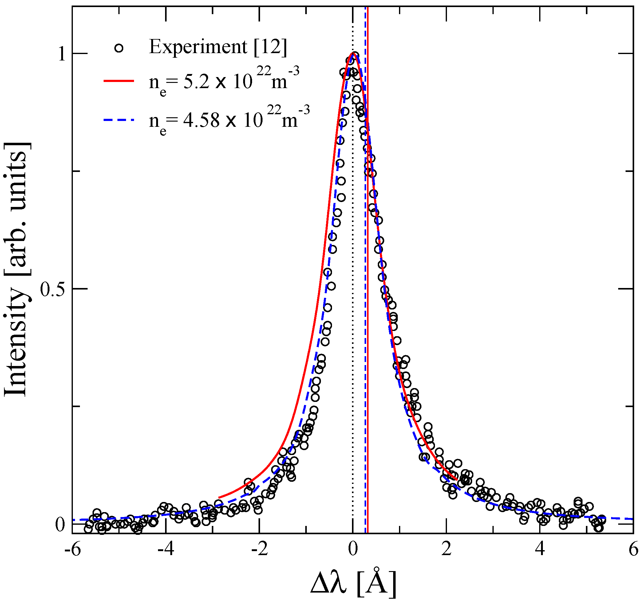
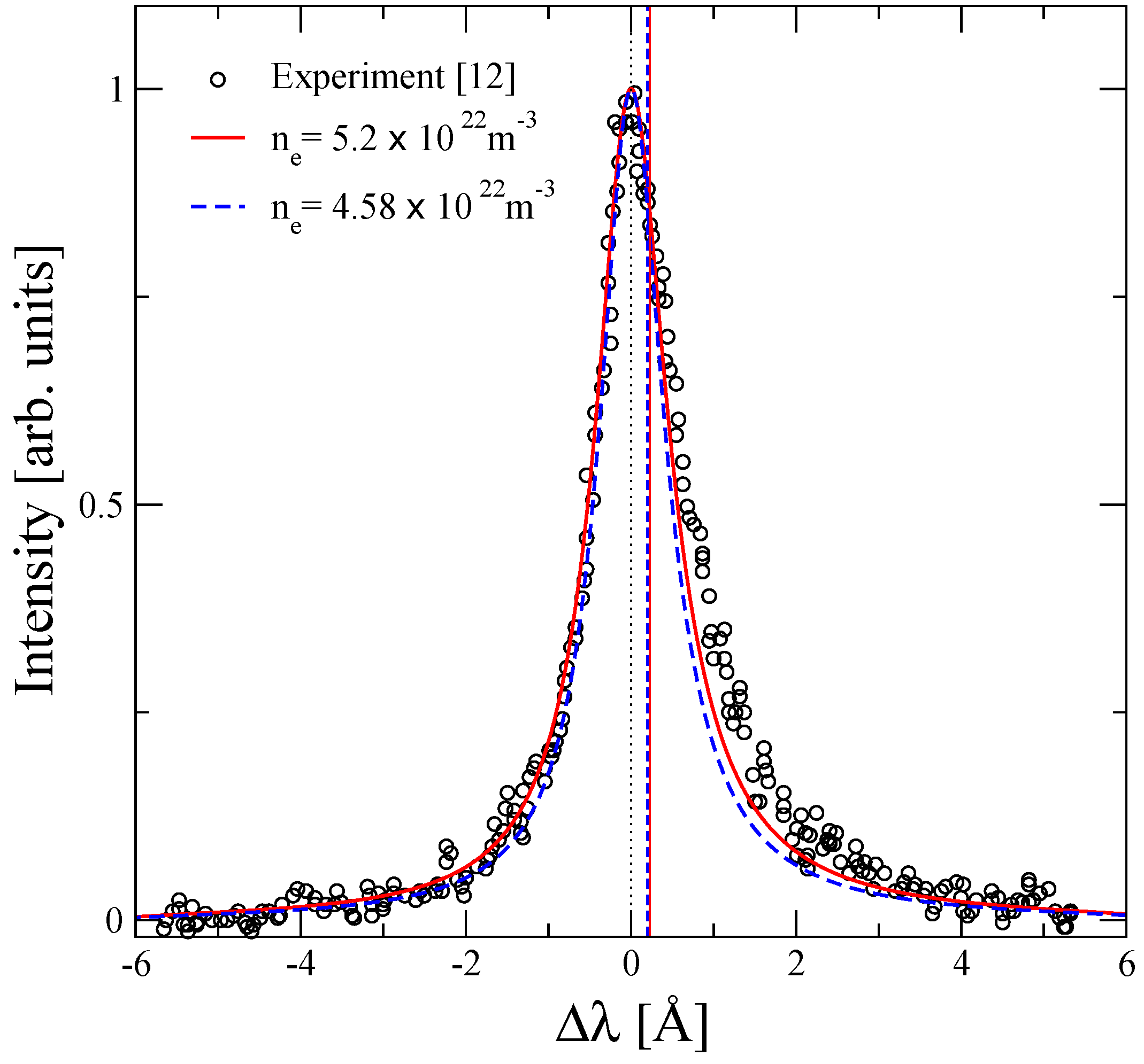
In this study, we present several theoretical approaches for calculating He I line shapes.The plasma parameters are inferred by comparing our results with the experimental measurement of Jovićević et al. [12]. The measured profile is compared with the theoretical profiles at $T=3.3\times {10}^4$ K for two values of electron densities $n_e=5.2\times {10}^{22}{\mathrm{m}}^{-3}$ and $n_e=4.58\times {10}^{22}{\mathrm{m}}^{-3}$, respectively. In [12] the experimental He I 3889 Å line broadening was fitted by using the $j_{AR}(x)$ line profiles generated on the assumption of electron impact broadening combined with broadening by quasistatic ion field using the ST of Griem [1]. The electron density of $n_e=4.8\times {10}^{22}{\mathrm{m}}^{-3}$ with an estimated uncertainty of $\pm 10\%$ was determined from the line broadening, while the electron temperature of $T=3.3\times {10}^4$ K with an uncertainty of $\pm 12\%$ was estimated by using the relative intensities of O II impurity lines.

In our quantum statistical approach electrons and ions are treated separately. Green’s function is applied for calculating the electronic contribution from Equation (3), while the dominant ionic contribution arises from the quadratic Stark effect and quadrupole interaction [15,16]. First, the ionic contribution is determined in the quasistatic approximation by using the calculated microfield distribution function in Section 3.1.2, then the new FFM formulation [18] is adopted to account for the fluctuation of the microfield on the spectral line shapes. The dynamic effects of the ionic motion are taken into account by substituting the area-normalized static profile into Equation (15). The result is displayed in Figure 1, which compares measured and theoretical profiles. Since the authors of the original experimental paper [12] did not mention any measurement of absolute line shift, we displaced the calculated line profiles to the unperturbed wavelength ${\lambda }_0=3888.65$ Å in Figure 1, Figure 2 and Figure 3 to determine the free electron density $n_e$ from the line width.

Figure 1. The calculated He I ($2^{3}S$–$3^{3}P$) line profiles in dynamically screened Born approximation by including ion dynamics in the FFM . Comparison is made with the measured data by Jovićević et al. [12] at $T=3.3\times {10}^4$ K. The profiles are plotted at the unperturbed transition wavelength ${\lambda }_0=3888.65$ Å, and the shift of profiles are shown.

Figure 1. The calculated He I ($2^{3}S$–$3^{3}P$) line profiles in dynamically screened Born approximation by including ion dynamics in the FFM . Comparison is made with the measured data by Jovićević et al. [12] at $T=3.3\times {10}^4$ K. The profiles are plotted at the unperturbed transition wavelength ${\lambda }_0=3888.65$ Å, and the shift of profiles are shown.

The electronic contribution is recalculated via the T-matrix by applying the CCC method in order to describe the strong electron-helium collisions within the Debye static screening model [34]. Both real and imaginary part of forward scattering amplitudes are substituted in Equation (4) to provide electronic shift and width [19]. In contrast to the Born approximation, the contribution of each state is different for different values of the magnetic quantum number $\left|m\right|=0,1$. Furthermore, an average over different spin-scattering channels $S=0$ and $S=1$ has been done. The Stark profiles are calculated in the quasistatic approximation from Equation (1) by using the T-matrix approach for electron-emitter collisions, The dynamic profiles are evaluated from Equation (15) and illustrated in Figure 2. It may be seen that the electron density $n_e=5.2\times {10}^{22}{\mathrm{m}}^{-3}$ gives better agreement with the experimental profile in Figure 1 and Figure 2.

Results from simulations are presented in Figure 3. Dynamic profiles show very good agreement with the measured profile for the inferred plasma density $n_e=4.58\times {10}^{22}{\mathrm{m}}^{-3}$ and temperature $T=3.3\times {10}^4$ K. In Table 1, numerical results of the shift and FWHM from our theories are given. We compare the broadening parameters in the dynamically screened Born approximation, the T-matrix approach, and MD simulations for interacting particles.

Figure 2. Comparison between the measured [12] and calculated line shapes of He I ($2^{3}S$–$3^{3}P$) using the T-matrix approach with ion dynamics in the FFM at $T=3.3\times {10}^4$ K. The profiles are given at the unperturbed transition wavelength ${\lambda }_0=3888.65$ Å, and the shift of profiles are shown.

Figure 2. Comparison between the measured [12] and calculated line shapes of He I ($2^{3}S$–$3^{3}P$) using the T-matrix approach with ion dynamics in the FFM at $T=3.3\times {10}^4$ K. The profiles are given at the unperturbed transition wavelength ${\lambda }_0=3888.65$ Å, and the shift of profiles are shown.

Figure 3. The calculated He I ($2^{3}S$–$3^{3}P$), line profiles from MD simulations compared with the experimental result of Jovićević et al. [12] at $T=3.3\times {10}^4$ K. The profiles are given at the unperturbed transition wavelength ${\lambda }_0=3888.65$ Å, and the shift of profilesare shown.

Figure 3. The calculated He I ($2^{3}S$–$3^{3}P$), line profiles from MD simulations compared with the experimental result of Jovićević et al. [12] at $T=3.3\times {10}^4$ K. The profiles are given at the unperturbed transition wavelength ${\lambda }_0=3888.65$ Å, and the shift of profilesare shown.

Figure 4. The shift of He I 3889 Å vs. electron density. Comparison between our calculated data and the experimental results are shown. The electron temperature is given for the corresponding T-matrix data points.

Figure 4. The shift of He I 3889 Å vs. electron density. Comparison between our calculated data and the experimental results are shown. The electron temperature is given for the corresponding T-matrix data points.

Ion dynamics (FFM) are included in the Born approximation and the T-matrix approach, the dynamic effects lead to further shift. The shift is significantly affected by including strong collisions via the T-matrix and ion-dynamics, while the dynamic profiles appear slightly broadened compared to the static profile. The calculated line shift for different values of $n_e$ is illustrated in Figure 1, Figure 2 and Figure 3 as well. Note, that the shift of this line is red, towards larger wavelengths with respect to the unperturbed transition line at ${\lambda }_0$. An example of the line measurement can be seen also in [50].

Table 1. Theoretical calculations of shift and FWHM of the He I 3889 Å line are illustrated in [Å], to analyze the experimental result of Jovićević et al. [12]. The calculated values correspond to dynamically screened Born approximation (quasistatic/FFM), T-matrix approach (quasistatic/FFM) and MD simulations at $T=3.3\times {10}^4$ K.

$n_e$ ${10}^{22}{\mathrm{m}}^{-3}$	Shift [Å]			FWHM [Å]
	Born	T-Matrix	MD	Born	T-Matrix	MD
5.2	0.483/0.523	0.178/0.228	0.32	1.245/1.278	1.038/1.087	1.402
4.58	0.427/0.462	0.147/0.197	0.269	1.094/1.123	0.914/0.965	1.245

Table 1. Theoretical calculations of shift and FWHM of the He I 3889 Å line are illustrated in [Å], to analyze the experimental result of Jovićević et al. [12]. The calculated values correspond to dynamically screened Born approximation (quasistatic/FFM), T-matrix approach (quasistatic/FFM) and MD simulations at $T=3.3\times {10}^4$ K.

$n_e$ ${10}^{22}{\mathrm{m}}^{-3}$	Shift [Å]			FWHM [Å]
	Born	T-Matrix	MD	Born	T-Matrix	MD
5.2	0.483/0.523	0.178/0.228	0.32	1.245/1.278	1.038/1.087	1.402
4.58	0.427/0.462	0.147/0.197	0.269	1.094/1.123	0.914/0.965	1.245

The illustrated approaches can provide the shift and full width at half maximum (FWHM) in a wide range of $n_e$ and T. The comparison with different measurements for shift and FWHM as a function of electron density $n_e\approx ({10}^{22}-{10}^{24}){\mathrm{m}}^{-3}$ in temperature range $T\approx (2-6)\times {10}^4$ K are shown in Figure 4 and Figure 5, respectively. The microfield distribution function of Hooper [51] is used in both the Born approximation and the T-matrix method for evaluating the Stark parameters in Figure 4 and Figure 5 [19]. However, outside the validity range of Hooper’s approach, we used the fit formula of Potekhin et al. [52] in our previous calculations in [19,53], which is based on Monte Carlo simulations and is appropriate for strongly coupled plasmas as well. The calculated FWHM in the T-matrix approach shows good agreement with the MD simulations data, especially at high densities. The ion dynamics slightly affects the width. However, the shift is rapidly reduced at low electron densities, and the discrepancy can be seen in contrast to MD simulations, but still the contribution of FFM is more pronounced in this region. The shift of this line is overestimated in the Born approximation compared to both the T-matrix method and MD simulations. The correlation between perturbers tends to decrease the line shift and width at high electron densities for interacting particles. In Figure 4 and Figure 5 the comparison is made with the following experiments: The measurement by Pérez et al. [54] was done in a low-pressure pulsed arc, in the plasma density range of $n_e=(1-6)\times {10}^{22}{\mathrm{m}}^{-3}$ and temperature interval of $T=(0.8-3)\times {10}^4$ K with a mean value of $2\times {10}^4$ K . The error bar of $n_e$ was $\pm 10\%$, and uncertainty in the temperature evaluation was about $20\%$. The experimental result of Kelleher [55] was obtained in a helium plasma generated in a wall-stabilized arc, with $n_e=1.03\times {10}^{22}{\mathrm{m}}^{-3}$ and $T_e=2.09\times {10}^4$ K. Recently, the FWHM of the same transition line was measured by Gao et al. [56] from a helium arc for the density range $n_e=(0.5-4)\times {10}^{22}{\mathrm{m}}^{-3}$ at $T=2.3\times {10}^4$ K. The reported result by Kobilarov et al. [57] from a pulsed low-pressure arc at $n_e=(2-10)\times {10}^{22}{\mathrm{m}}^{-3}$ and $T=(3.1-4.2)\times {10}^4$ K are included. Furthermore, values for the shift measured by Morris and Cooper [58] within the density range $n_e=(0.6-2.3)\times {10}^{22}{\mathrm{m}}^{-3}$ and $T=(1-1.6)\times {10}^4$ K are shown. The Stark parameters of this line were also measured by Berg et al. [59] at $n_e=1.5\times {10}^{22}{\mathrm{m}}^{-3}$ and $T_e=2.6\times {10}^4$ K. The measured widths by Milosavljević and Djeniže [60] are included as well, by using a linear low-pressure pulsed arc. The measured electron density and temperature were in the ranges of $(4.4-8.2)\times {10}^{22}{\mathrm{m}}^{-3}$ and $(1.8-3.3)\times {10}^4$ K with error bars $\pm 9\%$ and $\pm 10\%$, respectively. Furthermore, a comparison is made with the measurement of Soltwisch and Kusch [61], a wall-stabilized quasistationary pulsed discharge was used as a homogeneous plasma source. The spectra were recorded in a single shot, and the electron density range of $(0.7-1.2)\times {10}^{23}{\mathrm{m}}^{-3}$ was determined from the plasma reflectivity at two different wavelengths. The estimation of the temperature was about $2\times {10}^4$ K.

As shown in Figure 5, the T-matrix approach always gives a smaller FWHM than the Born approximation. This trend leads to a better agreement with the MD simulations results for interacting particles. For the data of Pérez et al. [54], the calculated width in the T-matrix approach agrees very well with the result of the Born approximation. However, the measurement may be influenced by self-absorption, as mentioned in [54], and then the measured widths may be overestimated. At $n_e=9.8\times {10}^{22}{\mathrm{m}}^3$, the width in the Born approximation shows a very good agreement with both measurement and MD simulations for independent particle data. However, the results of T-matrix approach and MD simulations for interacting particles give slightly lower values than the experiment data. At the highest measured density, the FWHM of theories is below that of Berg et al. [59]. Good agreement is found between the MD simulations result and T-matrix approach. However, the shift of this line is overestimated in the Born approximation, where, the strong collisions with large momentum transfer are not treated appropriately, while the perturbation theory breaks down at small distances and the perturbative expansion has to be avoided [20].

Figure 5. The FWHM of He I 3889 Å as a function of electron density. Our theoretical approaches are compared with the experiments results.

Figure 5. The FWHM of He I 3889 Å as a function of electron density. Our theoretical approaches are compared with the experiments results.

5. Conclusions

Spectral line shapes for He I are investigated theoretically in dense plasmas, the comparison is made with the measurements of Jovićević et al. [12] for diagnostic purposes. Free electron-emitter collisions are considered within both the Born approximation, and the T-matrix approach while ions are treated by the quasistatic approximation. The electronic contribution to the shift and width is computed by thermodynamic Green’s function by using Born approximation, which is the main contribution to the line broadening. Dynamic screening of the electron-atom interaction is included, which is a collective, many-particle effect. In contrast to ST, this effect modifies the broadening parameters with increasing free electron density, causing a non-linear behavior, where the plasma oscillations become relevant, see Figure 4 and Figure 5. A cut-off procedure for strong collisions is used according to Griem [1], while the second-order Born approximation overestimated the electronic contribution and the strong collisions term are added [23]. The Coulomb approximation is employed to evaluate the wavefunctions of helium. The accuracy of this approximation was approved for He-like ion by comparing our result with the Hartree-Fock wavefunctions, thus the radial part of transition matrix-element from various approaches were compared in [62].

Then the electron-emitter interaction is investigated again by elastic scattering amplitudes in Debye plasmas from a two-particle T-matrix approach by using the close-coupling equations. The Debye–Hückel potential significantly affects the bound states and scattering processes of the metastable states. The result is improved by treating strong electron-helium collisions consistently within T-matrix approach and better agreement can be seen with the measurement than the Born approximation, especially for the line shift. The contribution of perturbing ions is taken into account in a quasistatic approximation, with both quadratic Stark effect and quadrupole interaction. The perturbing ionic microfield is considered as a static field during the radiation. The calculated spectral line shapes in the static limit are modified by applying the FFM for both the Born approximation and T-matrix approach, which provides the dynamic line shapes and leads to further broadening [18]. In addition, MD simulations are used for comparison with the experiments and the analytically obtained profiles.

The shift of this line is over estimated in Born approximation even with a cut-off procedure and better agreement can be seen with the screened T-matrix approach and MD simulations. The FWHM of all theoretical approaches are in good agreement with the experimental result.

References

1. Griem, H.R. Spectral Line Broadening by Plasmas; Academic Press: New York, NY, USA, 1974. [Google Scholar]
2. Günter, S.; Hitzschke, L.; Röpke, G. Hydrogen spectral lines with the inclusion of dense-plasma effects. Phys. Rev. A 1991, 44, 6834–6844. [Google Scholar] [CrossRef] [PubMed]
3. Frisch, U.; Brissaud, A. Theory of Stark broadening soluble scalar model as a test. J. Quant. Spectrosc. Radiat. Transf. 1971, 11, 1753–1766. [Google Scholar] [CrossRef]
4. Seidel, J. Hydrogen Stark Broadening by Model Electronic Microfields. Z. Naturforschung A 1977, 32a, 1195–1206. [Google Scholar] [CrossRef]
5. Seidel, J. Effects of Ion Motion on Hydrogen Stark Profiles. Z. Naturforschung A 1977, 32a, 1207–1214. [Google Scholar] [CrossRef]
6. Stehlé, C.; Hutcheon, R. Extensive tabulations of Stark broadened hydrogen line profiles. Astron. Astrophys. Suppl. Ser. 1999, 140, 93–97. [Google Scholar] [CrossRef]
7. Talin, B.; Calisti, A.; Godbert, L.; Stamm, R.; Lee, R.W.; Klein, L. Frequency-fluctuation model for line-shape calculations in plasma spectroscopy. Phys. Rev. A 1995, 51, 1918–1928. [Google Scholar] [CrossRef] [PubMed]
8. Stamm, R.; Smith, E.W.; Talin, B. Study of hydrogen Stark profiles by means of computer simulation. Phys. Rev. A 1984, 30, 2039–2046. [Google Scholar] [CrossRef]
9. Gigosos, M.A.; Cardeñoso, V. New plasma diagnosis tables of hydrogen Stark broadening including ion-dynamics. J. Phys. B Atom. Mol. Opt. Phys. 1996, 29, 4795–4838. [Google Scholar] [CrossRef]
10. Gigosos, M.A.; González, M.A. Stark broadening tables for the helium I 447.1 line. Application to weakly coupled plasmas diagnostics. Astron. Astrophys. 2009, 503, 293–299. [Google Scholar] [CrossRef]
11. Gigosos, M.A.; Djurovic, S.; Savic, I.; González-Herrero, D.; Mijatovic, Z.; Kobilarov, R. Stark broadening of lines from transition between states n = 3 to n = 2 in neutral helium. An experimental and computer-simulation study. Astron. Astrophys. 2014, 561, A135:1–A135:13. [Google Scholar]
12. Jovićević, S.; Ivković, M.; Zikic, R.; Konjević, N. On the Stark broadening of Ne I lines and static vs. ion impact approximation. J. Phys. B Atom. Mol. Opt. Phys. 2005, 38, 1249–1259. [Google Scholar] [CrossRef]
13. Hitzschke, L.; Röpke, G.; Seifert, T.; Zimmermann, R. Green’s function approach to the electron shift and broadening of spectral lines in non-ideal plasmas. J. Phys. B Atom. Mol. Opt. Phys. 1986, 19, 2443–2456. [Google Scholar] [CrossRef]
14. Günter, S. Optische Eigenschaften Dichter Plasmen. Habilitation thesis, Rostock University, Rostock, Germany, 1995. [Google Scholar]
15. Sorge, S.; Wierling, A.; Röpke, G.; Theobald, W.; Sauerbrey, R.; Wilhein, T. Diagnostics of a laser-induced dense plasma by Hydrogen-like Carbon spectra. J. Phys. B Atom. Mol. Opt. Phys. 2000, 33, 2983–3000. [Google Scholar] [CrossRef]
16. Omar, B.; Günter, S.; Wierling, A.; Röpke, G. Neutral helium spectral lines in dense plasmas. Phys. Rev. E 2006, 73, 056405:1–056405:13. [Google Scholar] [CrossRef]
17. Günter, S.; Könies, A. Shifts and asymmetry parameters of hydrogen Balmer lines in dense plasmas. Phys. Rev. E 1997, 55, 907–911. [Google Scholar] [CrossRef]
18. Calisti, A.; Mossé, C.; Ferri, S.; Talin, B.; Rosmej, F.; Bureyeva, L.A.; Lisitsa, V.S. Dynamic Stark broadening as the Dicke narrowing effect. Phys. Rev. E 2010, 81, 016406:1–016406:6. [Google Scholar] [CrossRef]
19. Lorenzen, S.; Omar, B.; Zammit, M.C.; Fursa, D.V.; Bray, I. Plasma pressure broadening forfew-electron emitters including strong electron collisions within a quantum-statistical theory. Phys. Rev. E 2014, 89, 023106:1–023106:13. [Google Scholar] [CrossRef]
20. Hitzschke, L.; Günter, S. The influence of many-particle effects beyond the Debye approximation on spectral line shapes in dense plasmas. J. Quant. Spectrosc. Radiat. Transf. 1996, 56, 423–441. [Google Scholar] [CrossRef]
21. Beauchamp, A.; Wesemael, F.; Bergeron, P. Spectroscopicstudies of tudies DB white dwarfs: Improved Stark profiles for optical transitions of neutral helium. Astrophys. J. Suppl. Ser. 1997, 108, 559–573. [Google Scholar] [CrossRef]
22. Bates, D.R.; Damgaard, A. The calculation of the absolute strengths of spectral lines. Phil. Trans. Roy. Soc. Lond. A 1949, 242, 101–122. [Google Scholar] [CrossRef]
23. Griem, H.R.; Baranger, M.; Kolb, A.C.; Oertel, G. Stark broadening of neutral helium lines in a plasma. Phys. Rev. 1962, 125, 177–195. [Google Scholar] [CrossRef]
24. Halenka, J. Asymmetry of hydrogen lines in plasmas utilizing a statistical description of ion-quadruple interaction in Mozer-Baranger limit. Z. Phys. D 1990, 16, 1–8. [Google Scholar] [CrossRef]
25. Kraeft, W.-D.; Kremp, D.; Ebeling, W.; Röpke, G. Quantum Statistics of Charged Particle Systems; Akademie-Verlag: Berlin, Germany, 1986. [Google Scholar]
26. Günter, S. Contributions of strong collisions in the theory of spectral lines. Phys. Rev. E 1993, 48, 500–505. [Google Scholar] [CrossRef]
27. Baranger, M. General impact theory of pressure broadening. Phys. Rev. 1958, 112, 855–865. [Google Scholar] [CrossRef]
28. Bray, I.; Stelbovics, A.T. Convergent close-coupling calculations of electron-hydrogen scattering. Phys. Rev. A 1992, 46, 6995–7011. [Google Scholar] [CrossRef] [PubMed]
29. Fursa, D.V.; Dmitry, V.; Bray, I. Calculation of electron-helium scattering. Phys. Rev. A 1995, 52, 1279–1297. [Google Scholar] [CrossRef] [PubMed]
30. Bray, I.; Fursa, D.V.; Kadyrov, A.S.; Stelbovics, A.T.; Kheifets, A.S.; Mukhamedzhanov, A.M. Electron- and photon-impact atomic ionisation. Phys. Rep. 2012, 520, 135–174. [Google Scholar] [CrossRef]
31. Debye, P.; Hückel, E. Phys. Zeitschrift 1923, 24, 185–206.
32. Kardar, M. Statistical Physics of Particles; Cambridge University Press: Cambridge, UK, 2007; pp. 268–273. [Google Scholar]
33. Zammit, M.C.; Fursa, D.V.; Bray, I. Convergent-close-coupling calculations for excitation and ionization processes of electron-hydrogen collisions in Debye plasmas. Phys. Rev. A 2010, 82, 052705:1–052705:7. [Google Scholar] [CrossRef]
34. Zammit, M.C.; Fursa, D.V.; Bray, I.; Janev, R.K. Electron-helium scattering in Debye plasmas. Phys. Rev. E 2011, 84, 052705:1–052705:15. [Google Scholar] [CrossRef]
35. Bray, I.; Fursa, D.V. Benchmark cross sections for electron-impact total single ionization of helium. J. Phys. B Atom. Mol. Opt. Phys. 2011, 44(6), 061001:1–061001:3. [Google Scholar] [CrossRef]
36. Griaznov, V.K. Thermophysical Properties of the Working Gas of the Gas-Phase Nuclear Reactors; Atomizdat: Moscow, Russia, 1980. [Google Scholar]
37. Kudrin, L.P. Statistical Plasma Physics; Atomizdat: Moscow, Russia, 1974. [Google Scholar]
38. Ecker, G.; Müller, K.G. Plasmapolarisation und Trägerwechselwirkung. Z. Phys. 1958, 153, 317–330. [Google Scholar] [CrossRef]
39. Iglesias, C.A.; Hooper, C.F. Quantum corrections to the low-frequency-component microfield distributions. Phys. Rev. A 1982, 25, 1049–1059. [Google Scholar] [CrossRef]
40. Iglesias, C.A. Integral-equation method for electric microfield distribution. Phys. Rev. A 1983, 27, 2705–2709. [Google Scholar] [CrossRef]
41. Ramazanov, T.S.; Dzhumagulova, K.N. Effective screened potentials of strongly coupled semiclassical plasma. Phys. Plasmas 2002, 9, 3758–3761. [Google Scholar] [CrossRef]
42. Anderson, P.W. Pressure broadening in the microwave and infra-red regions. Phys. Rev. 1949, 76, 647–661. [Google Scholar] [CrossRef]
43. Gigosos, M.A.; González, M.A.; Cardeñoso, V. Computersimulated Balmer-alpha, -beta and -gamma Stark line profiles for non-equilibrium plasmas diagnostics. Spectrochim. Acta Part B 2003, 58, 1489–1504. [Google Scholar] [CrossRef]
44. Seidel, J.; Stamm, R. Effects of radiator motion on plasma-broadened hydrogen Lyman-β. J. Quant. Spectrosc. Radiat. Transfer 1982, 27, 499–503. [Google Scholar] [CrossRef]
45. González, M.A.; Gigosos, M.A. Analysis of Stark line profiles for non-equilibrium plasma diagnosis. Plasma Sourc. Sci. Technol. 2009, 18(3), 034001:1–034001:5. [Google Scholar] [CrossRef]
46. Bruggeman, P.; Schram, D.; González, M.A.; Rego, R.; Kong, M.G.; Leys, C. Characterization of a direct dc-excited discharge in water by optical emission spectroscopy. Plasma Sourc. Sci. Technol. 2009, 18(2), 025017:1–025017:13. [Google Scholar] [CrossRef]
47. Xiong, Q.; Nikiforov, A.Y.; González, M.A.; Leys, C.; Lu, X.P. Characterization of an atmospheric helium plasma jet by relative and absolute optical emission spectroscopy. Plasma Sourc. Sci. Technol. 2013, 22(1), 015011:1–025017:13. [Google Scholar] [CrossRef]
48. Dufour, E.; Calisti, A.; Talin, B.; Gigosos, A.M.; González, M.A.; Dufty, J.W. Charge correlation effects in electron broadening of ion emitters in hot and dense plasmas. J. Quant. Spectros. Radiat. Transf. 2003, 81, 125–132. [Google Scholar] [CrossRef]
49. Dufour, E.; Calisti, A.; Talin, B.; Gigosos, M.A.; González, M.A.; del Rio Gaztelurrutia, T.; Dufty, J.W. Charge-charge coupling effects on dipole emitter relaxation within a classicalelectron-ion plasma description. Phys. Rev. E 2005, 71, 066409:1–066409:9. [Google Scholar] [CrossRef]
50. Konjević, N.; Ivković, M.; Jovićević, S. Spectroscopic diagnostics of laser-induced plasmas. Spectrochim. Acta Part B: Atom. Spectrosc. 2010, 65, 593–602. [Google Scholar] [CrossRef]
51. Hooper, C.F., Jr. Low-frequency component electric microfield distributions in plasmas. Phys. Rev. 1968, 165, 215–222. [Google Scholar] [CrossRef]
52. Potekhin, A.Y.; Chabrier, G.; Gilles, D. Electric microfield distributions in electron-ion plasmas. Phys. Rev. E 2002, 65, 036412:1–036412:12. [Google Scholar] [CrossRef]
53. Omar, B.; Wierling, A.; Günter, S.; Röpke, G. Analysing brilliance spectra of a laser-induced carbon Plasma. J. Phys. A: Math. Gen. 2006, 39, 4731–4737. [Google Scholar] [CrossRef]
54. Pérez, C.; Santamarta, R.; de la Rosa, M.I.; Mar, S. Stark broadening of neutral helium lines and spectroscopic diagnostics of pulsed helium plasma. Eur. Phys. J. D 2003, 27, 73–75. [Google Scholar]
55. Kelleher, D.E. Stark broadening of visible neutral helium lines in a plasma. J. Quantit. Spectrosc. Radiat. Transf. 1981, 25, 191–220. [Google Scholar] [CrossRef]
56. Gao, H.M.; Ma, S.L.; Xu, C.M.; Wu, L. Measurements of electron density and Stark width of neutral helium lines in a helium arc plasma. Eur. Phys. J. D 2008, 47, 191–196. [Google Scholar] [CrossRef]
57. Kobilarov, R.; Konjević, N.; Popović, M.V. Influence of ion dynamics on the width and shift of isolated He I lines in plasmas. Phys. Rev. A 1989, 40, 3871–3879. [Google Scholar] [CrossRef] [PubMed]
58. Morris, R.N.; Cooper, J. Stark Shifts of He I 3889, He I 4713, and He I 5016. Can. J. Phys. 1973, 51, 1746–1751. [Google Scholar] [CrossRef]
59. Berg, H.F.; Ali, A.W.; Lincke, R.; Griem, H.R. Measurement of stark profiles of neutral and ionized helium and hydrogen lines from shock-heated plasmas in electromagnetic T tubes. Phys. Rev. 1962, 125, 199–206. [Google Scholar] [CrossRef]
60. Milosavljević, V.; Djeniže, S. Ion contribution to the astrophysical important 388.86, 471.32 and 501.56 nm He I spectral lines broadening. New Astron. 2002, 7, 543–551. [Google Scholar] [CrossRef]
61. Soltwisch, H.; Kusch, H.J. Experimental Stark profile Determination of some Plasma Broadened He I- and He II Lines. Z. Naturforsch. A 1979, 34a, 300–309. [Google Scholar] [CrossRef]
62. Omar, B.; Wierling, A.; Reinholz, H.; Röpke, G. Diagnostic of laser induced Li II plasma. Phys. Rev. Res. Int. 2013, 3, 218–227. [Google Scholar]
63. Röpke, G.; Seifert, T.; Kilimann, K. A Green’s function approach to the shift of spectral lines in dense. Ann. Phys. (Leipzig) 1981, 38, 381–460. [Google Scholar] [CrossRef]
64. Kobzev, G.A.; Iakubov, I.T.; Popovich, M.M. Transport and Optical Properties of Nonideal Plasmas; Plenum Press: New York, NY, USA & London, UK, 1995. [Google Scholar]
65. Redmer, R. Physical properties of dense, low-temperature plasmas. Phys. Rep. 1997, 282, 35–157. [Google Scholar] [CrossRef]
66. Günter, S. Stark shift and broadening of hydrogen spectral lines. Contrib. Plasma Phys. 1989, 29, 479–487. [Google Scholar] [CrossRef]
67. Kadanoff, L.P.; Baym, G. Quantum Statistical Mechanics: Green’s Function Methods in Equilibrium and Nonequilibrium Problems; Addison-Wesley Publishing Co., Inc.: New York, NY, USA, 1989. [Google Scholar]
68. Zimmermann, R. Many Particle Theory of Highly Excited Semiconductors; BSB Teubner: Leipzig, Germany, 1987. [Google Scholar]
69. Zimmermann, R.; Kilimann, K.; Kraeft, W.-D.; Kremp, D.; Röpke, G. Dynamical screening and self energy of excitons in the electron-hole plasma. Phys. Stat. Sol. (B) 1978, 90, 175–187. [Google Scholar] [CrossRef]
70. Omar, B. Spectral line broadening in dense plasmas. J. Atom. Mol. Opt. Phys. 2011, 2011, 850807:1–850807:8. [Google Scholar] [CrossRef]
71. Edmonds, A.R. Angular Momentum in Quantum Mechanics; Princeton University Press: Princeton, NJ, USA, 1960. [Google Scholar]