
Fundamental Features of Quantum Dynamics Studied in Matter-Wave Interferometry—Spin Weak Values and the Quantum Cheshire-Cat


Abstract
:
1. Introduction
2. Neutron Interferometer Experiments in History
3. Spin Weak Measurements
3.1. Theoretical Framework
3.2. Neutron Optical Approach
3.3. Experimental Results
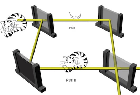
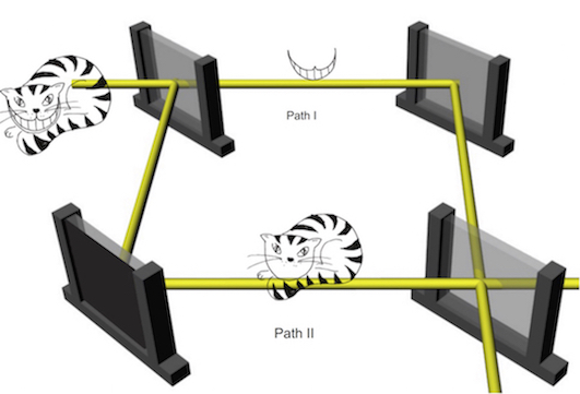
4. The Quantum Cheshire-Cat
4.1. Theory
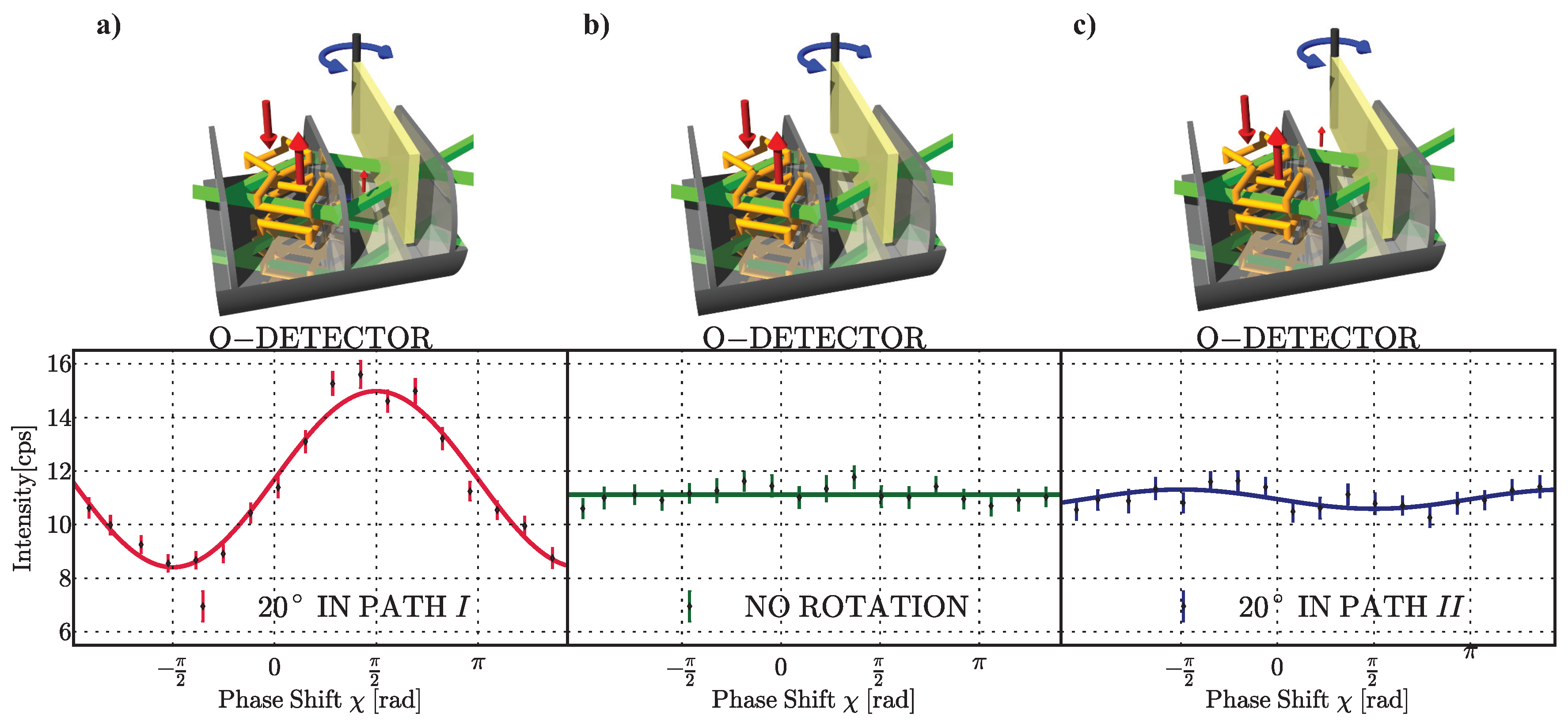
4.2. Experiment
5. Conclusions
Acknowledgments
Author Contributions
Conflicts of Interest
Abbreviations
| AAV | Aharonov, Albert and Vaidman |
| AB | Aharonov-Bohm |
| AC | Aharonov-Casher |
| DC | direct current |
| DOF | degrees of freedom |
| GHZ | Greenberger-Horne-Zeilinger |
| ILL | Institute Laue-Langevin |
| IFM | interferometer |
| LLL | triple Laue |
| RF | radio frequency |
| VCN | very cold neutrons |
References
- Tonomura, A. Applications of electron holography. Rev. Mod. Phys. 1987, 59, 639–669. [Google Scholar] [CrossRef]
- Feynman, R.; Leighton, R.; Sands, M. The Feynman Lectures on Physics, 2nd ed.; Addison-Wesley: Boston, MA, USA, 1963; Volume 1. [Google Scholar]
- Arndt, M.; Ekers, A.; von Klitzing, W.; Ulbricht, H. Focus on modern frontiers of matter wave optics and interferometry. New J. Phys. 2012, 14, 125006. [Google Scholar] [CrossRef]
- Cronin, A.D.; Schmiedmayer, J.; Pritchard, D.E. Optics and interferometry with atoms and molecules. Rev. Mod. Phys. 2009, 81, 1051–1129. [Google Scholar] [CrossRef]
- Popescu, S. Dynamical quantum non-locality. Nat. Phys. 2010, 6, 151–153. [Google Scholar] [CrossRef]
- Bertlmann, R.A.; Zeilinger, A. Quantum [Un]speakables, from Bell to Quantum Information; Springer Verlag: Heidelberg, Germany, 2002. [Google Scholar]
- Maier-Leibnitz, H.; Springer, T. Ein Interferometer für langsame Neutronen. Z. Phys. 1962, 167, 386. [Google Scholar] [CrossRef]
- Mezei, F. Neutron spin echo: A new concept in polarized thermal neutron techniques. Z. Phys. 1972, 25, 146. [Google Scholar] [CrossRef]
- Rauch, H.; Treimer, W.; Bonse, U. Test of a single crystal neutron interferometer. Phys. Lett. A 1974, 47, 369–371. [Google Scholar] [CrossRef]
- Rauch, H.; Werner, S.A. Neutron Interferometry; Clarendon Press: Oxford, UK, 2000. [Google Scholar]
- Rauch, H.; Zeilinger, A.; Badurek, G.; Wilfing, A.; Bauspiess, W.; Bonse, U. Verification of Coherent Spinor Rotation of Fermions. Phys. Lett. A 1975, 54, 425–427. [Google Scholar] [CrossRef]
- Werner, S.A.; Colella, R.; Overhauser, A.W.; Eagen, C.F. Observation of the Phase Shift of a Neutron Due to Precession in a Magnetic Field. Phys. Rev. Lett. 1975, 35, 1053–1055. [Google Scholar] [CrossRef]
- Klein, A.G.; Opat, G.I. Observation of 2π Rotations by Fresnel Diffraction of Neutrons. Phys. Rev. Lett. 1976, 37, 238–240. [Google Scholar] [CrossRef]
- Grigoriev, S.; Kraan, W.; Rekveldt, M.Th. Observation of 4-pi periodicity of the spinor using neutron resonance interferometry. Europhys. Lett. 2004, 66, 164–170. [Google Scholar]
- Colella, R.; Overhauser, A.W.; Werner, S.A. Observation of Gravitationally Induced Quantum Interference. Phys. Rev. Lett. 1975, 34, 1472–1474. [Google Scholar] [CrossRef]
- Sakurai, J.J. Modern Quantum Mechanics; Addison-Wesley: New York, NY, USA, 1994. [Google Scholar]
- Littrell, K.C.; Allman, B.E.; Werner, S.A. Two-wavelength-difference measurement of gravitationally induced quantum interference phases. Phys. Rev. A 1997, 56, 1767–1780. [Google Scholar] [CrossRef]
- Van der Zouw, G.; Weber, M.; Felber, J.; Gähler, R.; Geltenbort, P.; Zeilinger, A. Aharonov-Bohm and gravity experiments with the very-cold-neutron interferometer. Nucl. Instrum. Meth. A 2000, 440, 568–574. [Google Scholar] [CrossRef]
- Klepp, J.; Sponar, S.; Hasegawa, Y. Fundamental phenomena of quantum mechanics explored with neutron interferometers. Prog. Theor. Exp. Phys. 2014, 2014. [Google Scholar] [CrossRef]
- De Haan, V.O.; Plomp, J.; van Well, A.A.; Rekveldt, M.T.; Hasegawa, Y.H.; Dalgliesh, R.M.; Steinke, N.J. Measurement of gravitation-induced quantum interference for neutrons in a spin-echo spectrometer. Phys. Rev. A 2014, 89, 063611. [Google Scholar] [CrossRef]
- Nielsen, M.A.; Chuang, I. Quantum Computation and Quantum Information; Cambridge Unviversity Press: Cambridge, UK, 2000. [Google Scholar]
- Bell, J.S. On the Einstein-Podolsky-Rosen paradox. Physics 1964, 1, 195–200. [Google Scholar]
- Kochen, S.; Specker, E.P. The problem of hidden variables in quantum mechanics. J. Math. Mech. 1967, 17, 59–87. [Google Scholar] [CrossRef]
- Hasegawa, Y.; Loidl, R.; Badurek, G.; Baron, M.; Rauch, H. Violation of a Bell-like inequality in single-neutron interferometry. Nature 2003, 425, 45–48. [Google Scholar] [CrossRef] [PubMed]
- Geppert, H.; Denkmayr, T.; Sponar, S.; Lemmel, H.; Hasegawa, Y. Improvement of the polarized neutron interferometer setup demonstrating violation of a Bell-like inequality. Nucl. Instrum. Methods Phys. Res. Sect. A 2014, 763, 417–423. [Google Scholar] [CrossRef] [PubMed]
- Hasegawa, Y.; Loidl, R.; Badurek, G.; Baron, M.; Rauch, H. Quantum Contextuality in a Single-Neutron Optical Experiment. Phys. Rev. Lett. 2006, 97, 230401. [Google Scholar] [CrossRef] [PubMed]
- Cabello, A.; Filipp, S.; Rauch, H.; Hasegawa, Y. Proposed Experiment for Testing Quantum Contextuality with Neutrons. Phys. Rev. Lett. 2008, 100, 130404. [Google Scholar] [CrossRef] [PubMed]
- Bartosik, H.; Klepp, J.; Schmitzer, C.; Sponar, S.; Cabello, A.; Rauch, H.; Hasegawa, Y. Experimental Test of Quantum Contextuality in Neutron Interferometry. Phys. Rev. Lett. 2009, 103, 040403. [Google Scholar] [CrossRef] [PubMed]
- Greenberger, D.M.; Horne, M.A.; Zeilinger, A. Bell’s Theorem, Quantum Theory, and Concepts of the Universe; Kafatos, M., Ed.; Kluwer Academics: Dordrecht, The Netherlands, 1989; pp. 73–76. [Google Scholar]
- Greenberger, D.M.; Shimony, A.; Horne, M.A.; Zeilinger, A. Bell’s theorem without inequalities. Am. J. Phys. 1990, 58, 1131–1143. [Google Scholar] [CrossRef]
- Hasegawa, Y.; Loidl, R.; Badurek, G.; Durstberger-Rennhofer, K.; Sponar, S.; Rauch, H. Engineering of triply entangled states in a single-neutron system. Phys. Rev. A 2010, 81, 032121. [Google Scholar] [CrossRef]
- Erdösi, D.; Huber, M.; Hiesmayr, B.C.; Hasegawa, Y. Proving the generation of genuine multipartite entanglement in a single-neutron interferometer experiment. New J. Phys. 2013, 15, 023033. [Google Scholar] [CrossRef]
- Aharonov, Y.; Albert, D.Z.; Vaidman, L. How the result of a measurement of a component of the spin of a spin-1/2 particle can turn out to be 100. Phys. Rev. Lett. 1988, 60, 1351–1354. [Google Scholar] [CrossRef] [PubMed]
- Aharonov, Y.; Vaidman, L. Properties of a quantum system during the time interval between two measurements. Phys. Rev. A 1990, 41, 11–20. [Google Scholar] [CrossRef] [PubMed]
- Aharonov, Y.; Vaidman, L. The two-state vector formalism: an updated review. Lect. Nots. Phys. 2007, 734, 399–447. [Google Scholar]
- Aharonov, Y.; Bergmann, P.G.; Lebowitz, J.L. Time Symmetry in the Quantum Process of Measurement. Phys. Rev. 1964, 134, 1410–1416. [Google Scholar] [CrossRef]
- Ritchie, N.W.M.; Story, J.G.; Hulet, R.G. Realization of a measurement of a “weak value”. Phys. Rev. Lett. 1991, 66, 1107–1110. [Google Scholar] [CrossRef] [PubMed]
- Duck, I.M.; Stevenson, P.M.; Sudarshan, E.C.G. The sense in which a “weak measurement” of a spin-1/2 particle’s spin component yields a value 100. Phys. Rev. D 1989, 40, 2112–2117. [Google Scholar] [CrossRef]
- Hosten, O.; Kwiat, P. Observation of the Spin Hall Effect of Light via Weak Measurements. Science 2008, 319, 787–790. [Google Scholar] [CrossRef] [PubMed]
- Dixon, P.B.; Starling, D.J.; Jordan, A.N.; Howell, J.C. Ultrasensitive Beam Deflection Measurement via Interferometric Weak Value Amplification. Phys. Rev. Lett. 2009, 102, 173601. [Google Scholar] [CrossRef] [PubMed]
- Starling, D.J.; Dixon, P.B.; Jordan, A.N.; Howell, J.C. Precision frequency measurements with interferometric weak values. Phys. Rev. A 2010, 82, 063822. [Google Scholar] [CrossRef]
- Starling, D.J.; Dixon, P.B.; Williams, N.S.; Jordan, A.N.; Howell, J.C. Continuous phase amplification with a Sagnac interferometer. Phys. Rev. A 2010, 82, 011802. [Google Scholar] [CrossRef]
- Feizpour, A.; Xing, X.; Steinberg, A.M. Amplifying Single-Photon Nonlinearity Using Weak Measurements. Phys. Rev. Lett. 2011, 107, 133603. [Google Scholar] [CrossRef] [PubMed]
- Ota, Y.; Ashhab, A.; Nori, F. Entanglement amplification via local weak measurements. J. Phys. A 2012, 45, 415303. [Google Scholar] [CrossRef]
- Zhou, L.; Turek, Y.; Sun, C.P.; Nori, F. Weak-value amplification of light deflection by a dark atomic ensemble. Phys. Rev. A 2013, 88, 053815. [Google Scholar] [CrossRef]
- Kofman, A.G.; Ashhab, S.; Nori, F. Nonperturbative theory of weak pre- and post-selected measurements. Phys. Rep. 2012, 520, 43–133. [Google Scholar] [CrossRef]
- Kocsis, S.; Braverman, B.; Ravets, S.; Stevens, M.J.; Mirin, R.P.; Shalm, L.K.; Steinberg, A.M. Observing the Average Trajectories of Single Photons in a Two-Slit Interferometer. Science 2011, 332, 1170–1173. [Google Scholar] [CrossRef] [PubMed]
- Lundeen, J.S.; Sutherland, B.; Patel, A.; Stewart, C.; Bamber, C. Direct measurement of the quantum wavefunction. Nature 2011, 474, 188–191. [Google Scholar] [CrossRef] [PubMed]
- Goggin, M.E.; Almeida, M.P.; Barbieri, M.; Lanyon, B.P.; O’Brien, J.L.; White, A.G.; Pryde, G.J. Violation of the Leggett-Garg inequality with weak measurements of photons. Proc. Natl. Acad. Sci. USA 2011, 108, 1256–1261. [Google Scholar] [CrossRef] [PubMed]
- Salvail, J.Z.; Agnew, M.; Johnson, A.S.; Bolduc, E.; Leach, J.; Boyd, R.W. Full characterization of polarization states of light via direct measurement. Nat. Photonics 2013, 7, 316–321. [Google Scholar] [CrossRef]
- Dressel, J.; Malik, M.; Miatto, F.M.; Jordan, A.N.; Boyd, R.W. Colloquium: Understanding quantum weak values: Basics and applications. Rev. Mod. Phys. 2014, 86, 307–316. [Google Scholar] [CrossRef]
- Ozawa, M. Universally valid reformulation of the Heisenberg uncertainty principle on noise and disturbance in measurement. Phys. Rev. A 2003, 67, 042105. [Google Scholar] [CrossRef]
- Rozema, L.A.; Darabi, A.; Mahler, D.H.; Hayat, A.; Soudagar, Y.; Steinberg, A.M. Violation of Heisenberg’s Measurement-Disturbance Relationship by Weak Measurements. Phys. Rev. Lett. 2012, 109, 100404. [Google Scholar] [CrossRef] [PubMed]
- Ringbauer, M.; Biggerstaff, D.N.; Broome, M.A.; Fedrizzi, A.; Branciard, C.; White, A.G. Experimental Joint Quantum Measurements with Minimum Uncertainty. Phys. Rev. Lett. 2014, 112, 020401. [Google Scholar] [CrossRef] [PubMed]
- Kaneda, F.; Baek, S.Y.; Ozawa, M.; Edamatsu, K. Experimental Test of Error-Disturbance Uncertainty Relations by Weak Measurement. Phys. Rev. Lett. 2014, 112, 020402. [Google Scholar] [CrossRef] [PubMed]
- Dressel, J.; Nori, F. Certainty in Heisenberg’s uncertainty principle: Revisiting definitions for estimation errors and disturbance. Phys. Rev. A 2014, 89, 022106. [Google Scholar] [CrossRef]
- Resch, J.; Lundeen, J.; Steinberg, A. Experimental realization of the quantum box problem. Phys. Lett. A 2004, 324, 125–131. [Google Scholar] [CrossRef]
- Lundeen, J.S.; Steinberg, A.M. Experimental Joint Weak Measurement on a Photon Pair as a Probe of Hardy’s Paradox. Phys. Rev. Lett. 2009, 102, 020404. [Google Scholar] [CrossRef] [PubMed]
- Yokota, K.; Yamamoto, T.; Koashi, M.; Imoto, N. Direct observation of Hardy’s paradox by joint weak measurement with an entangled photon pair. New J. Phys. 2009, 11, 033011. [Google Scholar] [CrossRef]
- Aharonov, Y.; Botero, A.; Popescu, S.; Reznik, B.; Tollaksen, J. Revisiting Hardy’s paradox: counterfactual statements, real measurements, entanglement and weak values. Phys. Lett. A 2002, 301, 130–138. [Google Scholar] [CrossRef]
- Bliokh, K.Y.; Bekshaev, A.Y.; Kofman, A.G.; Nori, F. Photon trajectories, anomalous velocities and weak measurements: a classical interpretation. New J. Phys. 2013, 15, 073022. [Google Scholar] [CrossRef]
- Dressel, J.; Bliokh, K.Y.; Nori, F. Classical Field Approach to Quantum Weak measurements. Phys. Rev. Lett. 2014, 112, 110407. [Google Scholar] [CrossRef] [PubMed]
- Sponar, S.; Denkmayr, T.; Geppert, H.; Lemmel, H.; Matzkin, A.; Tollaksen, J.; Hasegawa, Y. Weak values obtained in matter-wave interferometry. Phys. Rev. A 2015, 92, 062121. [Google Scholar] [CrossRef]
- Wu, S.; Mølmer, K. Weak measurements with a qubit meter. Phys. Lett. A 2009, 374, 34–39. [Google Scholar] [CrossRef]
- Aharonov, Y.; Popescu, S.; Rohrlich, D.; Skrzypczyk, P. Quantum Cheshire Cats. New J. Phys. 2013, 15, 113015. [Google Scholar] [CrossRef]
- Denkmayr, T.; Geppert, H.; Sponar, S.; Lemmel, H.; Matzkin, A.; Tollaksen, J.; Hasegawa, Y. Experimental observation of a quantum cheshire cat in matter wave interferometry. Nat. Commun. 2014, 5, 4492. [Google Scholar] [CrossRef] [PubMed]
- Aharonov, Y.; Cohen, E. Weak Values and Quantum Nonlocality. 2015; arXiv:1504.03797. [Google Scholar]
- Danan, A.; Danan, D.; Bar-Ad, S.; Vaidman, L. Asking Photons Where They Have Been. Phys. Rev. Lett. 2013, 111, 240402. [Google Scholar] [CrossRef] [PubMed]


| Population | Magnetic Moment |
|---|---|
| = 0.14(4) | = 1.07(25) |
| = 0.96(6) | = 0.02(24) |
© 2016 by the authors; licensee MDPI, Basel, Switzerland. This article is an open access article distributed under the terms and conditions of the Creative Commons by Attribution (CC-BY) license (http://creativecommons.org/licenses/by/4.0/).
Share and Cite
Sponar, S.; Denkmayr, T.; Geppert, H.; Hasegawa, Y. Fundamental Features of Quantum Dynamics Studied in Matter-Wave Interferometry—Spin Weak Values and the Quantum Cheshire-Cat. Atoms 2016, 4, 11. https://doi.org/10.3390/atoms4010011
Sponar S, Denkmayr T, Geppert H, Hasegawa Y. Fundamental Features of Quantum Dynamics Studied in Matter-Wave Interferometry—Spin Weak Values and the Quantum Cheshire-Cat. Atoms. 2016; 4(1):11. https://doi.org/10.3390/atoms4010011
Chicago/Turabian StyleSponar, Stephan, Tobias Denkmayr, Hermann Geppert, and Yuji Hasegawa. 2016. "Fundamental Features of Quantum Dynamics Studied in Matter-Wave Interferometry—Spin Weak Values and the Quantum Cheshire-Cat" Atoms 4, no. 1: 11. https://doi.org/10.3390/atoms4010011