
Atom Interferometry in the Presence of an External Test Mass

1
1849 S. Ocean Dr, Apt. 207, Hallandale, FL 33009, USA
2
Physics Division, Physical and Life Sciences, Lawrence Livermore National Laboratory, Livermore, CA 94550, USA
3
Physics Department, University of Michigan, Ann Arbor, MI 48109, USA
*
Author to whom correspondence should be addressed.
Atoms 2016, 4(2), 14; https://doi.org/10.3390/atoms4020014
Submission received: 29 December 2015
/
Revised: 29 March 2016
/
Accepted: 6 April 2016
/
Published: 21 April 2016
(This article belongs to the Special Issue Atom Interferometry)
Abstract
:The influence of an external test mass on the phase of the signal of an atom interferometer is studied theoretically. Using traditional techniques in atom optics based on the density matrix equations in the Wigner representation, we are able to extract the various contributions to the phase of the signal associated with the classical motion of the atoms, the quantum correction to this motion resulting from atomic recoil that is produced when the atoms interact with Raman field pulses and quantum corrections to the atomic motion that occur in the time between the Raman field pulses. By increasing the effective wave vector associated with the Raman field pulses using modified field parameters, we can increase the sensitivity of the signal to the point where such quantum corrections can be measured. The expressions that are derived can be evaluated numerically to isolate the contribution to the signal from an external test mass. The regions of validity of the exact and approximate expressions are determined.
Keywords:
atom interferometry; inhomogeneous gravitational fields; test mass; quantum phase correctionsPACS:
03.75.Dg; 37.25.+k; 04.80.-y1. Introduction
Since its birth about 30 years ago [1], the field of atom interferometry (AI) has matured significantly. Experiments based on AI have been used to measure fundamental constants [2,3,4,5], the acceleration of gravity near the Earth’s surface [6,7,8,9], the gradient of the Earth’s gravitational field [4,10,11] and the curvature of the gravitational field produced by source masses [12]. Atom interferometer gyroscopes allow one to measure rotation rates; experiments have utilized optical fields [13], nanofabricated structures [14] and three or four spatially- or temporally-separated sets of fields that drive Raman transitions to split and recombine the matter waves [15,16,17,18]. The frequency shift arising from a quadratic Zeeman effect was also measured precisely [19]. There have been limits set on a non-Newtonian Yukawa-type fifth force [20] and on dark energy [21] using AI, as well as theoretical proposals for using AI to measure general relativity effects [22,23], including gravitational waves [24]. A detailed theoretical analysis of the combined effect of rotation and gravity on the AI signal has been given [17], based on three- and four-pulse Raman schemes.
Atom interferometry has also been used to probe the gravitational field produced by a heavy test mass [4,5,12,20,21]. Using a double-difference technique [4], one can extract that part of the phase of the AI signal caused by the gravitational field of the test mass. This article provides a theoretical calculation of this contribution to the phase, based on an atom interferometer using three Raman field pulses. The results can be used to optimize measurements of the Newtonian gravitational constant G and to provide a complete derivation of results outlined in a previous paper [25]. We might point out that an analytic, semi-classical expression for the phase response of an atom interferometer to an arbitrarily-placed, stationary point mass has been derived recently [26].
Estimated Phase Corrections Resulting from the Test Mass
The phase in an atom interferometer depends on the interactions of the atoms with the applied Raman fields, as well as the motion of the atoms between and following the applied Raman pulses. The Raman pulses couple two hyperfine sub-levels, g and e, in the atomic ground state manifold, and it is the phase associated with the Raman coherence that is measured using the interferometer. The presence of a gravitational potential modifies the atomic trajectories, leading to a modification of the AI phase. This modification of the phase serves as a measure of the sensitivity of AI to gravitational effects. Since the Earth’s gravitational potential is only slightly inhomogeneous over the physical extent of the atom interferometer, it can be approximated by a Taylor series in which only the lead and gradient terms are retained [27,28,29,30]. Approximate solutions for the atomic trajectories were obtained in [17,29], where effects related to the Earth’s rotation (centripetal and Coriolis forces) were also included. An exact expression for the atom trajectories with these combination of forces has also been derived for a non-spherical gravitational source (i.e., for an arbitrary gravity-gradient tensor), rotating with constant angular velocity [31].
The situation can change dramatically if a massive test object is brought close to the interferometer (see Figure 1). The accumulated phase produced by the test mass’ gravitational field, , increases with decreasing distance between the test mass and the trajectories of the atoms in the interferometer and also increases with increasing delay times T between the Raman pulses. For sufficiently long T and small , it is no longer a good approximation to retain only the lead and gradient terms when considering the gravitational potential associated with the test mass, as was done for the Earth’s gravitational potential.
The maximum value of T is limited by experimental considerations; the largest delay time that has been achieved is s [32]. Even for smaller delay times, the inhomogeneity of the field can be significant. For example, with ms, in a symmetric fountain geometry [33], the length of the atomic trajectory is longer than:
where is Earth’s gravitational field. With m (see Eqs. (103) and (104) in Section 3), the usually accepted assumption that the gravitational acceleration is constant or slightly inhomogeneous along the atom trajectory becomes invalid.
In calculating the atomic trajectories, we can assume [34] that the magnitude of the gravitational field of the test mass at the position of the atoms in the interferometer is much less than that of the Earth’s field [35],
Nevertheless, both the average field and field gradient associated with the test mass can modify the phase of the AI signal. Let us denote the average field of the test mass over the interferometric path as . The interferometric phase associated with this average field strength is of order [6,7,8,9]:
where k is an effective wave vector of the Raman field and T is the time delay between Raman pulses. This phase change arises owing to the acceleration of the atoms produced by the field of the test mass.
In addition to this “classical” contribution to the phase, there are quantum corrections whose effect we would now like to estimate. Atom interferometers that make use of copropagating optical fields or copropagating Raman pulses as their beam splitters and combiners have a signal phase that is insensitive to quantum corrections if the gravity field is homogeneous. Quantum corrections arise as a result of rotation [39] or inhomogeneous field terms [28,29]. Quantum corrections to the phase from an inhomogeneous gravitational field are of order:
where is an atomic mass and γ is the magnitude of the relevant terms in the gravity-gradient tensor. One can understand the estimate (4) as the quantum part of the phase addition [28,29,30] associated with the change of atomic velocity owing to recoil [36] after interaction with a Raman pulse. When the length of the atomic trajectory L becomes comparable to the characteristic distance over which the gravitational potential of the test mass changes, a reasonable estimate for γ is . As a consequence, we find:
For Rb m:
Calculations [25] indicate that can be as large as 1 rad, implying that can be as large as rad. Since a lower limit for the phase noise in the interferometer is of order [32]:
one sees that quantum corrections are small, but measurable; we will include them in our considerations.
Another type of quantum correction is produced during the free evolution of the atomic coherence between the Raman pulses. We formulate the problem in terms of the Wigner representation [37,38] for the atomic density matrix, . This is a standard approach for studying phenomena related to quantization of the atomic center of mass motion [36] and laser cooling [40]. However, to our knowledge, it has been used sparingly in the context of AI [17,41]. The convenience of this approach is that, for the time between Raman pulses, obeys an equation that is similar to the classical Liouville equation for the distribution function [37,38].
The Wigner distribution function can be written as,
where is the density matrix in the coordinate representation and is the density matrix in the momentum representation. To estimate the quantum corrections, we start from the time evolution equation for the Wigner function for times between the application of the Raman pulses. In the absence of the Earth’s rotation, this equation can be written as [17]:
where is the gravitational potential. For nearly homogeneous fields, such as the Earth’s field, the potential functions in Eq. (9b) can be expanded to first order in ℏ. In that limit, one finds that and that the Wigner function obeys the same Liouville equation as the classical density matrix in the time between pulses. In the presence of a test mass, however, the gravitational potential is strongly inhomogeneous, and higher order terms in the expansion are needed.
Let us estimate the correction from these higher order terms. If the term in the Liouville Equation (9a) is responsible for the phase in estimate (3), then the Q-term results in a quantum correction:
The density matrix depends on atomic momentum p in two characteristic ways. There is both a thermal momentum:
( is Boltzmann constant, is atom cloud temperature) and a momentum associated with the Doppler phase,
For Rb at temperature K, m, and ms,
where m/s is the thermal velocity. In qualitative terms, we can think of the dependence of on momentum to vary as:
where the first factor represents the thermal distribution and the second a phase factor resulting from the accumulated Doppler phase between Raman pulses. Explicit forms for the Doppler phase acquired by the Raman coherence in a time T are derived in the next section, but they are typically of order .
If , it follows that the Doppler phase factor makes the dominant contribution to the momentum gradient, since:
To estimate the quantum corrections, we expand Eq. (9b) to second order in ℏ to obtain:
Replacing by and by , we find:
Consistent with the phase noise given in Eq. (7), one should ignore the Q-term in Eq. (9a). However, if one uses the AI technique to measure the Newtonian gravitational constant G with an accuracy of several ppm (the level achieved is already 150 ppm [5]), then the Q-term should be included. Anticipating innovations capable of reducing the phase noise to rad [42], one has to include the Q-term. Consequently, we will include the corrections resulting from this term.
To summarize, there are two types of quantum corrections to the AI phase that are to be considered. The first, , arises from inhomogeneous gravitational field modifications of the Doppler phase associated with the recoil the atoms undergo on interacting with the Raman fields. The ratio is of order . The second, , arises from quantum corrections to the off-diagonal elements of the Wigner distribution during periods of free evolution. The ratio is of order .
It is possible to increase both and the quantum corrections and using larger values of the effective wave vector Moreover, since , and [see Eqs. (3), (4), (16)], the relative weight of the quantum corrections also increases with increasing k. There are at least five ways to increase k: the production of higher order atomic density harmonics in a standing wave field in the Raman–Nath regime (see Eq. (4) in [1]), higher order Bragg scattering [43], the sequential Bragg scattering technique [2], multicolor techniques [44] and Raman standing wave techniques [45]. For example, standing wave pulses in the Raman–Nath regime were used to produce the 10th harmonic of the atomic density without excessive loss of signal magnitude and without sub-recoil cooling [46]. A beam splitter was demonstrated using an extension of the Raman standing wave technique [47], and a beam splitter has been produced using higher order Bragg scattering [48]. Recently, a high order Bragg scattering atom interferometer was used to determine the fine structure constant with a resolution 0.25 ppb [3]. A beam splitter has been utilized for atom interference using sequential Bragg scattering [49]. On the theoretical side, it was shown that, with a proper choice of field polarization, Raman standing waves in the Raman–Nath regime can be used to create a beam splitter without increasing the number of separated Raman pulses [45,50]. To account for such enhancements, our calculations of the AI’s phase are carried out for an effective k-vector that is scaled by an integer factor
This article is arranged as follows. In the next section, we derive exact and approximate expressions for the phases , , and The results of numerical calculations of the phases are given in Section 3 for a stationary test mass and a test mass moving at constant velocity. The calculations enable us to establish the regions of validity of the approximate expressions for the phases.
2. Basic Formalism
The working medium of the atom interferometer consists of a cloud of atoms that are launched with some initial velocity at . The cloud interacts with three Raman pulses that are separated in time; these pulses couple two hyperfine sub-levels in the atomic ground state manifold. In the time intervals between the pulses, the atoms move under the influence of a gravitational potential . The cloud is assumed to be characterized by a Wigner distribution at time and is assumed to be sufficiently localized, such that, at any time, the gravitational field is the same for all atoms in the cloud. In other words, the cloud can be considered as a point insofar as it interacts with both the Earth’s and the test mass’ gravitational fields. The problem can be broken down into periods of “free evolution” of density matrix elements before the first Raman pulse is applied and for the time intervals between subsequent Raman pulses and into time intervals in which the Raman fields are applied. By “free evolution”, we mean evolution in the absence of applied radiation fields, but including the effects produced by . We consider each region separately and then piece together the total response.
We will see that the quantum corrections leading to originate in the recoil the atoms undergo as a result of their interaction with the Raman pulses. Following the interactions, this recoil leads to a contribution to the Doppler phase of the off-diagonal density matrix elements (g and e are sub-levels of the atoms’ ground state manifold) in the time intervals between the pulses. In addition, the momentum derivatives of the Doppler phase factors give rise to the Q-term corrections; as such, the Q-term corrections depend only on the free evolution of off-diagonal density matrix elements between the pulses.
2.1. Density Matrix Evolution between the Raman Pulses
Between the Raman pulses, the Wigner function evolves according to Eqs. (9). When the distance L over which the gravitational potential energy varies significantly is much larger than ℏ divided by the characteristic width of the momentum distribution, i.e.,
we can expand Q [Eq. (9b)] in a power series in ℏ to obtain:
where:
A summation convention implicit in Eq. (18) will be used in all subsequent equations. Repeated indices and symbols appearing on the right-hand side (rhs) of an equation are to be summed over, unless they also appear on the left-hand side (lhs) of that equation.
We have already shown in Eq. (16) that the Q-term can be considered as a small perturbation, allowing us to write:
where is the unperturbed density matrix obeying the equation:
and is a perturbation whose evolution is governed by the equation:
The term contains the corrections, while the term provides the corrections.
Equation (21) has been studied in [17] for the Earth’s gravitational field. In this article, we obtain a solution of Eq. (21) in the presence of a test mass and solve Eq. (22) to get the contribution to the AI phase arising from the Q-term. We assume that the density matrix is known at some preceding time and arbitrarily set at this time, such that, at . The solution of the homogeneous Eq. (21) is then given by [17]:
where are the atomic classical position and momentum at time subject to the constraint that the position and momentum are specified by at time In other words, in Eq. (23), we look for the values for which will lead to values under the influence of the gravitational fields.
Turning our attention to Eq. (22), we see that the curly brackets in that equation are a total time derivative, enabling us to write:
Integrating this equation from equals to using the fact that , and making use of Eqs. (18), (19) and (23), , we find
Using Eq. (23) one more time, we arrive at:
2.2. Changes in Density Matrix Elements Produced by the Raman Pulses
Consider now a cloud of atoms having two hyperfine sub-levels g and e in the ground state manifold. The atoms are prepared in level g at time , and they proceed to interact with the sequence of Raman pulses applied at times:
where is time delay between cloud launch and the first Raman pulse and T is the time delay between pulses. The initial atomic density matrix (8) is given by:
where is the Wigner distribution at
Similarly, for π-pulse applied at time ,
In these equations, is an effective wave vector (assumed to be the same for all of the pulses); is the detuning between the hyperfine transition frequency and the effective frequency of the Raman fields (the effective frequency is the frequency difference of the two fields used to create the Raman pulse); is the phase difference between traveling components of the Raman field; and are times just after and before the pulse. We allow pulses to have different detunings and phases ().
It is assumed that the temporal width of the Raman pulses is sufficiently short to guarantee that all phases related to the detuning, Doppler shifts and the gravitational fields are effectively frozen during the application of the pulses. In addition, we assume that the Raman field amplitude and phase are constant over the size of the atomic cloud, allowing us to neglect corrections arising from the ac -Stark effect and wave front curvature of the Raman fields. In principle, most of these assumptions are not necessary. One can derive and explore the analogue of Eqs. (29) and (30) considering extended atom clouds at finite temperature, including corrections arising from Doppler broadening, ac-Stark effects and gravitational acceleration produced during the Raman pulses. In this case, however, the corrections depend on the initial atomic distribution Since this distribution is usually not known accurately, it is preferable for high precision atomic interferometry to use Raman pulses of sufficiently short duration, sufficiently large diameter and sufficiently flat wave fronts to avoid such corrections.
If a pulse acts on a ground state atom, it produces a superposition of ground and excited states. If there were a momentum associated with the ground state amplitude before the pulse is applied, the excited state amplitude depends on . As a consequence, the off-diagonal density matrix element following the pulse involves the product of state amplitudes evolving with different momenta. It is this difference in momentum that leads to the Q-term correction in periods of free evolution.
2.3. AI Signal
Our goal is to calculate , the excited state atomic density matrix element following the third Raman pulse, since can be related to experimentally-measurable quantities. To carry out the calculation, we use Eqs. (23) and (26) for the “free evolution” of density matrix elements before the first Raman pulse is applied and for the time intervals between subsequent Raman pulses and use Eqs. (29) and (30) for changes in the density matrix elements resulting from the application of the Raman pulses. In these free evolution regions, density matrix elements are affected by the presence of a gravitational potential that ultimately contributes to the phase of the AI signal.
From the time the cloud is launched at to the time that the first Raman pulse is applied, the only non-vanishing density matrix element is . In the time interval between and , this density matrix element evolves to:
For reasons to be discussed below, corrections from the Q-term can be neglected in this time interval. After the first -pulse, the density matrix elements change to:
One uses these density matrix elements as initial values for the free evolution between the first and second pulses of the unperturbed density matrix; that is,
We now consider the modifications produced by the Q-term in the time interval between the first and second pulses. The modifications produced by the Q-term (26) in the atomic coherence before the second pulse acts, , can be calculated from Eqs. (26), (32c) and (33) as:
In Eq. (34), the π derivatives lead to two types of terms. The first of these originates from the thermal distribution and is of order:
where is thermal momentum defined in Eq. (11). The second arises from the phase factor in Eq. (34), evaluated at To estimate this contribution, we “turn off” the gravitational field. In this approximation:
and the Doppler phase becomes equal to This phase factor is a rapidly oscillating function of momentum π having period of order defined by Eq. (12), from which we find:
In the limit that:
the thermal derivative is smaller than the Doppler derivative by the ratio given in Eq. (13) and can be neglected.
When inequality (38) holds, the time separation between pulses T is sufficiently large to ensure that the dominant contributions to the Q-term comes from the momentum derivatives of the Doppler phase factor. As we will show, the atomic levels’ populations ( and ) have no phase factor for ; therefore, the Q-term corrections arise only from the atomic coherence As a consequence, we can neglect any contribution to the Q-term corrections from atomic state populations. It was for this reason that we did not include any Q-term corrections to the Wigner distribution for the time interval . In the Doppler limit defined by Eq. (38), the AI phase is pretty much independent of the atomic momentum and spatial distributions.
Calculating the derivatives and retaining those contributions to the derivatives arising from the Doppler phase only, we arrive at:
where is the u-th component of the effective k-vector. In this approximation, the derivative no longer acts on the term inside the curly brackets. Therefore, we can apply the multiplication law,
to get:
The expression inside the curly brackets of Eq. (39) becomes t-independent, and the Q-term just before the second pulse is given by:
We still need an expression for the time evolution of between the first and second pulses. From Eqs. (23), (32) and (40), we find:
At time , the π pulse acts, which, according to Eqs. (30), transforms these density matrix elements at time into:
The next step is to calculate the Q-term corrections in time interval Each density matrix element in Eqs. (44) produces a Q-term correction. However, the diagonal matrix elements given by Eqs. (44a) and (44b) contain no rapidly oscillating phase factors in momentum space, allowing us to neglect their Q-term corrections. Moreover, Eq. (44d) is already linear in Q and can produce only higher order corrections that we neglect in this work. As a consequence, we need consider only the Q-term correction produced by the coherence in Eq. (44c), which we denote as From Eq. (26), we find:
where we used the multiplication law (40),
In Eq. (45), the differentiation over momentum π is carried out only for the Doppler phase factors. After differentiation, we apply the multiplication law two more times to the phase factor and distribution f, namely:
for and find that these terms become t-independent. As a result, one gets for the Q-term before the third pulse,
The value of will depend both on and In other words, we must also calculate the time evolution of and between the second and third pulses. Applying Eq. (23), we find:
Combining the different contributions to the off diagonal density matrix element given by Eqs. (48), (49c) and (49d) and factoring out a common phase factor, we obtain:
Finally, we use Eqs. (29a), (49a), (49b) and (50) to calculate following the pulse at time as:
This density matrix element can be used to calculate any physically-measured observable associated with atoms in state e. For example, one could measure the state e population given as:
The first two terms in Eq. (51) are responsible for the background signal. When substituted into Eq. (52), they yield a background contribution equal to , allowing us to write:
where the interferometric term is given by:
To carry out the integration, we express all position and momenta in terms of the position and momentum variables at Time 0, denoted by:
In terms of these variables,
After redefining , one finds:
where the phase of the AI is defined as:
with given by Eq. (50c).
2.3.1. Atom Trajectories in the Presence of the Test Mass
To calculate the phases in Eqs. (58), we need expressions for the propagation functions , i.e., atomic position and momentum at time t subject to the initial value at time . These functions evolve as:
We neglect in Eqs. (59) the gravity-gradient, centrifugal and Coriolis forces caused by the rotating Earth. When is a perturbation, the approximate solutions of Eqs. (59) are [34]:
Each of the functions obeys the multiplication law (40):
2.3.2. Phases
It remains for us to calculate the phases and . In the following two subsections, we obtain both exact integral and approximate integral and analytic expressions for these phases. In Section 3, the exact expressions are evaluated numerically, and the range of validity of the approximate expressions is established.
The phase includes a “classical” part (non-vanishing in the limit , as well as a quantum correction . The contributions to resulting from the Earth’s gravitational field and the rotation of the Earth were calculated approximately in [17,29]. The classical component of these contributions to has been calculated exactly [31]. In this paper, we concentrate on the additions to caused by the test mass’ field. The “classical” part of this addition has been evaluated in [25]. Contributions to the phase from the Earth’s rotation and Earth’s gravity-gradient terms are neglected in this paper.
It is shown in the Appendix how approximate expressions for the propagators needed in Eq. (58b) can be obtained from Eqs. (60). It then follows that the phase given in Eq. (58b) can be written as a sum of three terms,
The term is the classical contribution from the Earth’s field; the term is the classical contribution from the test mass’ field; and the term is the quantum correction arising from the test mass’ field.
To evaluate the classical contribution to the phase given by Eq. (62c), we use Eq. (60e) to arrive at:
Eqs. (62c) and (63) have been used in [25]. With the simple change of variables, for and for , we find:
If the test mass moves without rotation and follows a trajectory denoted by , then:
and:
This is the exact expression for ψ that is used in Section 3.
We can arrive at an approximate expression for ψ if we assume that the distance between the atoms and the test mass is sufficiently large to keep only those terms that are linear in the field gradient. In other words, we can evaluate the field of the test mass at some average displacement between the test mass and the atoms’ trajectory. If we choose [51]:
expand:
where is the gravity-gradient tensor having matrix elements:
and substitute the result back into Eq. (66), we find that the term proportional to vanishes ( was chosen to ensure this). We then obtain an approximate expression for the classical contribution to the phase given by:
We now turn our attention to the quantum correction. The vector given in Eq. (62g) can be rewritten as:
Substituting in the first term of Eq. (71) and in the second term, we obtain:
For translational motion, when the gravitational field of the test mass is given by Eq. (65),
This is the exact expression for that is used in Section 3.
There are two approximate expressions we will derive for ψ. When the recoil effect is small,
we can expand the arguments in Eq. (73) to obtain a first approximation given by:
where:
For translational motion of the test mass, , and Eq. (75b) reduces to:
The second approximate expression we obtain for is the limit of Eq. (77) when the distance between the atoms and the test mass is sufficiently large to keep only those terms that are linear in the field gradient. If we choose:
and expand:
where:
is an element of the gravity curvature tensor, then the contribution from the second term in Eq. (79) vanishes, and we find an approximate expression for the phase given by:
We now consider Q-term quantum corrections to the phase given by Eqs. (58c) and (50c). We first replace by in Eq. (50c) to obtain:
allowing us to write as:
When atoms move between the Raman pulses under the action of the homogeneous gravitational field of the Earth and the inhomogeneous perturbation caused by the test mass, the only contribution to (defined in Eq. (19)) results from the presence of the test mass,
where:
Since we calculate the AI phase to first order in , it is sufficient to calculate the atom trajectory in Eq. (83) to zeroth order in , i.e., to set:
which results in:
where is a Kronecker delta. Moreover, since we are interested in calculating to second order in the recoil momentum , we can neglect the contribution of the recoil term in the braces of Eq. (83). We then apply the multiplication law (40) and obtain:
As before, we transform the integral to one from zero to T,
If the test mass moves without rotation, then:
and:
This is the exact expression for that is used in Section 3.
We can obtain an approximate expression for when the distance between the atoms and the test mass is sufficiently large to keep only those terms that are linear in the field curvature. If we choose:
and expand:
the contribution to the Q-term from the second term in Eq. (93) vanishes, and we find an approximate expression for the phase given by:
3. Point Source Test Mass
For a point source test mass M moving along the trajectory , the gravitational field, gravity-gradient tensor and gravity curvature tensor are given by:
where mkg·s is the Newtonian gravitational constant.
We numerically calculated the classical part of the phase given by Eqs. (62c) and (66) (for ) and the quantum corrections given by Eqs. (62d) and (73) (for ) and (91) (for ) and determined when these terms become measurable in the presence of phase noise given by Eq. (7). Moreover, we checked the validity of the approximate expressions given in Eqs. [(70), (67)], (77), [(81),(78)], and [(94),(92)]. The results vary with the test mass’ weight, shape, trajectory, as well as with the operating parameters of the atom interferometer.
The calculations are carried out for a test mass moving with constant velocity ,
where:
is the location of the test mass at time
We assume that, at , the atoms are launched from the origin of the north-east-down frame in the vertical direction. That is, it is assumed that is in the positive z-direction and that the cloud position is given by:
where is the launch velocity, taken to be along the z-axis. In this case, one finds from Eqs. (60c), (67), (78) and (92) that:
Recall that these values were chosen to ensure that the first order terms vanish in the expansions given in Eqs. (68), (79) and (93). As such, by expanding the expressions for ψ about these points, we obtained approximate expressions with corrections of order times derivatives of the gravity gradient tensor, derivatives of the gravity-curvature tensor and second derivatives of the gravity-curvature tensor for , and , respectively. As such, these choices improve the accuracy of the approximations.
The launch velocity is chosen as:
corresponding to a symmetric fountain geometry in which the atomic cloud reaches its highest point at time , when the second pulse is applied. Calculations have been performed for a stationary test mass having:
and a test mass moving with constant velocity along the x-axis,
The parameters characterizing the atom interferometer, the test mass and the Earth’s field are summarized in Table 1. Since the cloud trajectory and the effective wave vectors are vertical, can be considered as an “impact parameter” for the test mass relative to the cloud trajectory along the z-axis.
Equations (95) can be used either for a point mass or a spherical mass having constant density ρ and radius:
For the highest density in nature, 22,600 kg/m, corresponding to osmium [52],
For impact parameters Eqs. (95) are valid only for those values of for which atom trajectory does not intersect the spherical test mass. In the case of a stationary sphere, this requirement translates into one in which the distance between the cloud and the sphere is always greater than ; that is, for any :
With given by Eq. (98a) and given by Eq. (100), we can show that this inequality is satisfied if:
For the moving sphere, the range of allowed initial positions for the center of the sphere is more difficult to calculate. For this reason, in Case 2, we consider only impact parameters larger than the sphere’s radius, , for which, evidently, any values of are allowed.
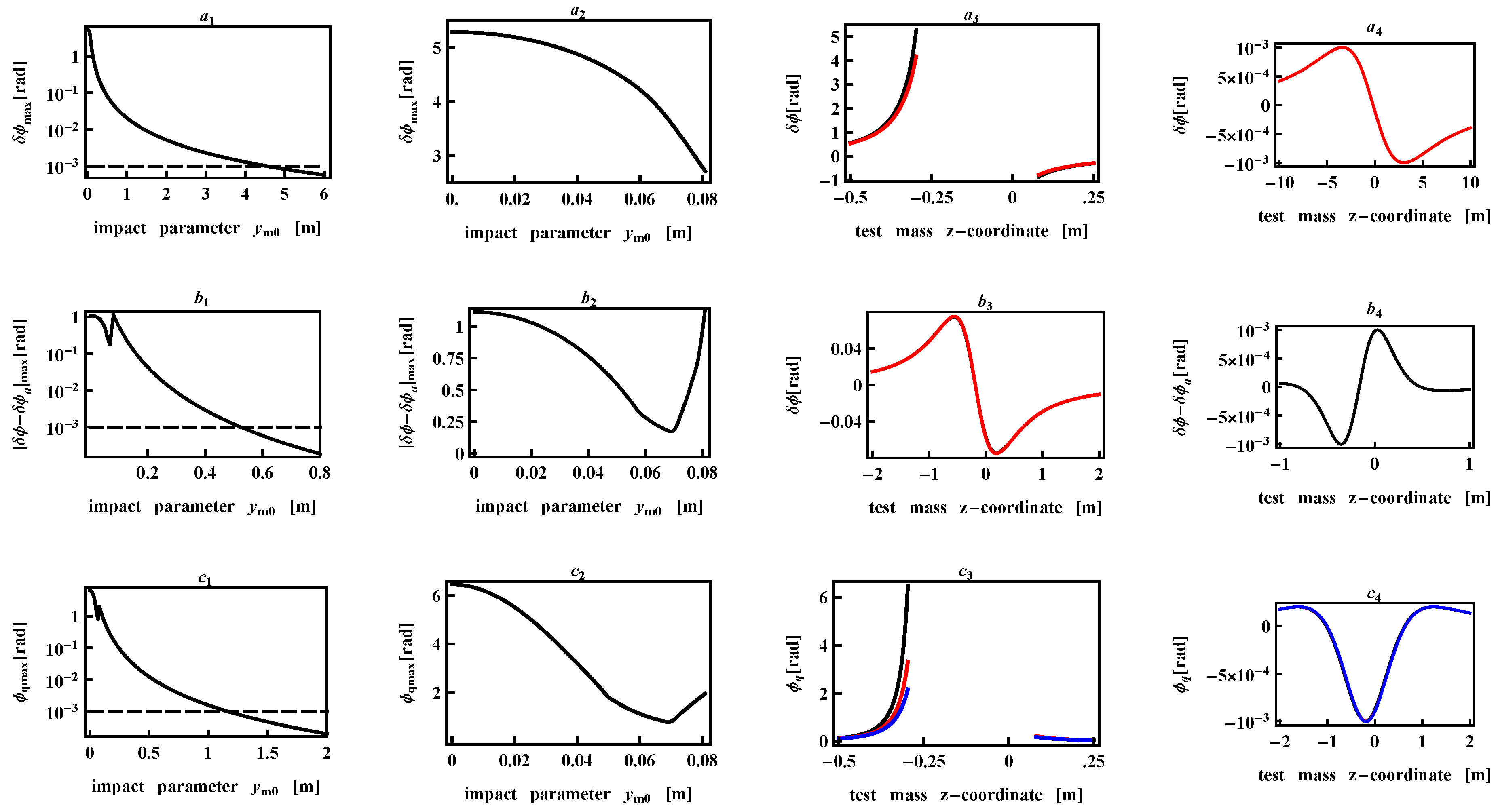
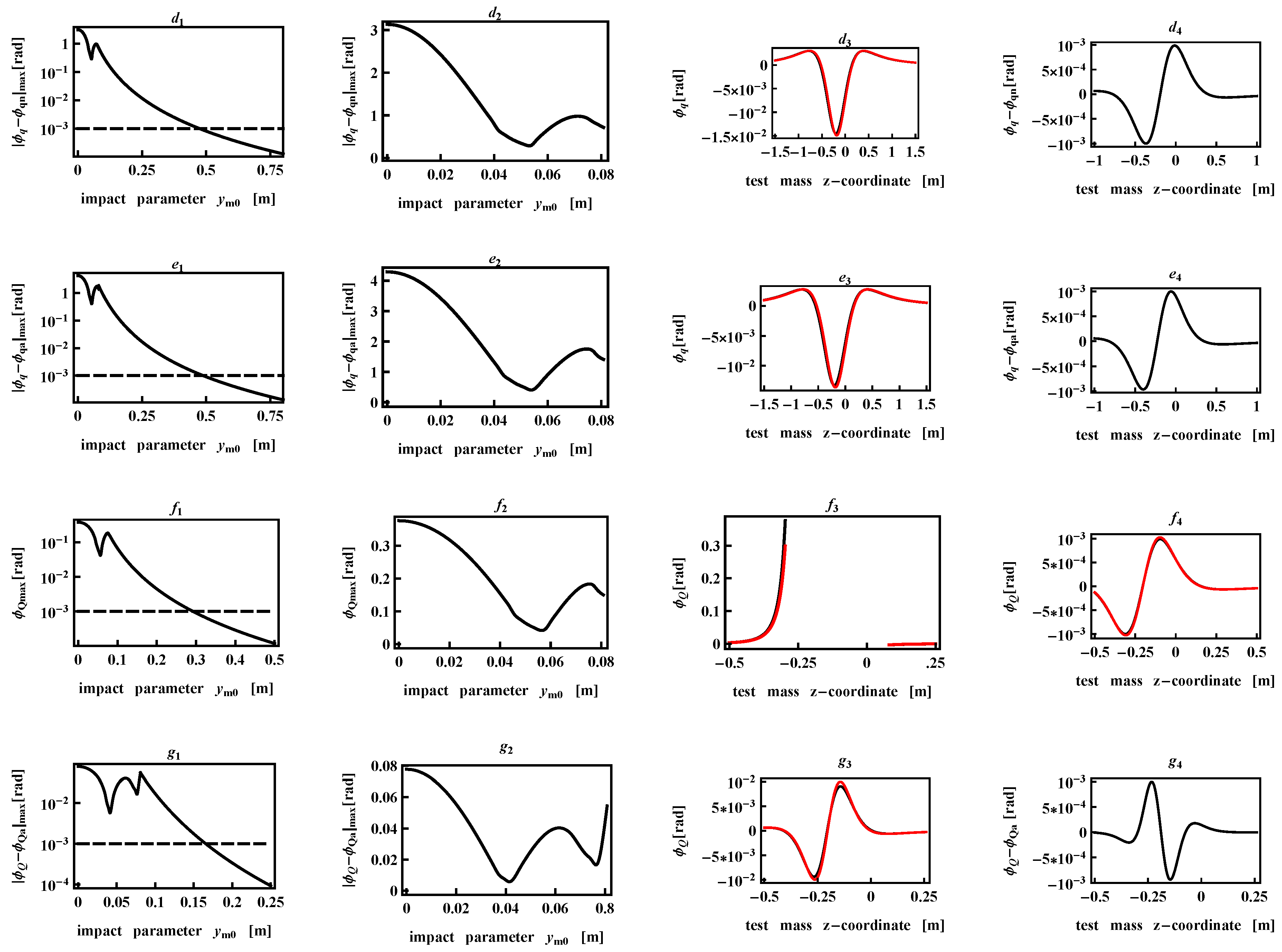
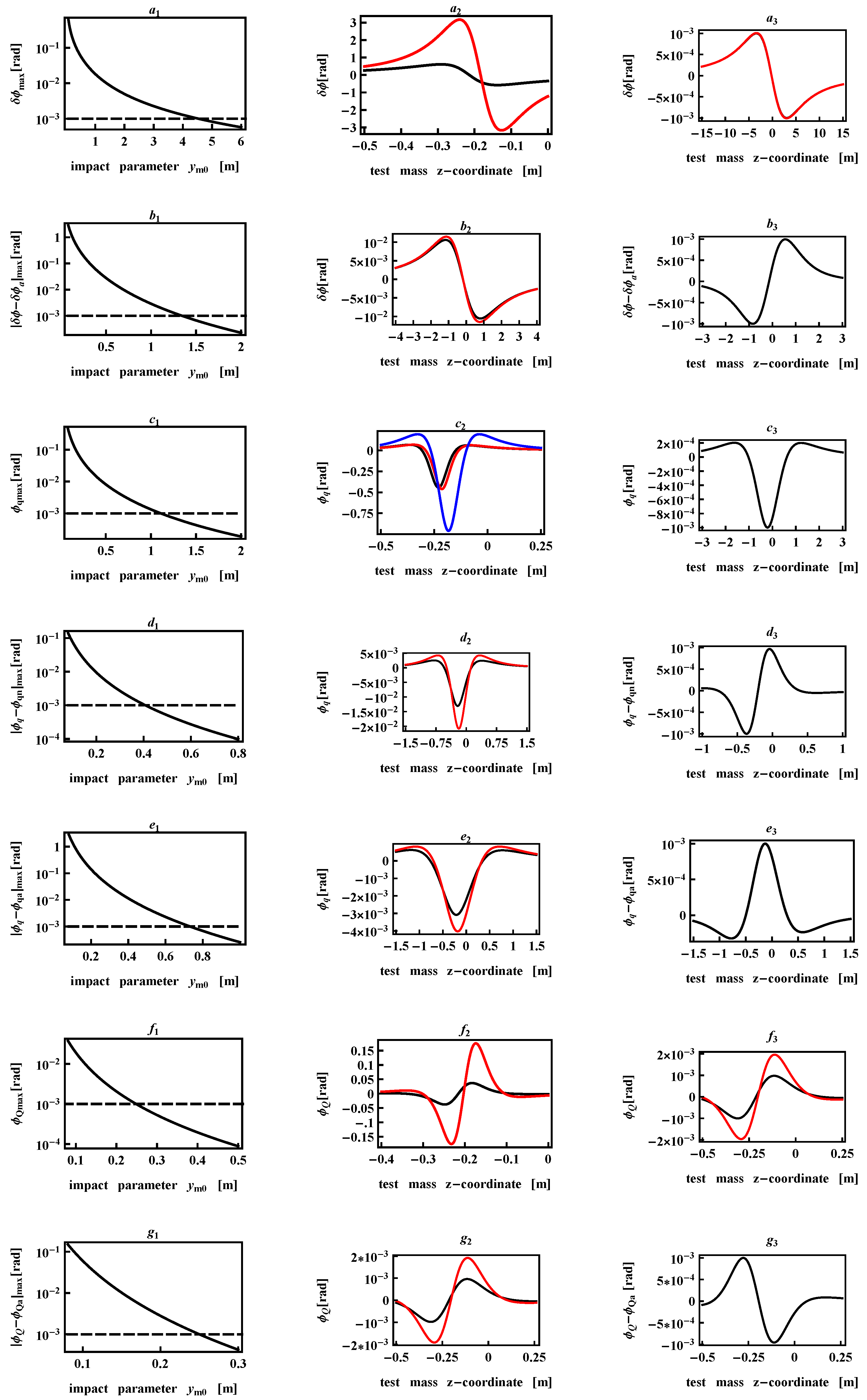
For each impact parameter and for the parameters given in Table 1, we explore various test mass positions and trajectories. The results of the calculations are illustrated graphically in Figure 2 for a stationary mass and in Figure 3 for a mass moving at constant velocity. Although the various plots may be difficult to read at standard magnification, they can be read easily using the zoom feature when read online in PDF format.
In the first two columns of Figure 2, we plot:
- (1)
- maximum of the magnitude of the phase obtained from Eqs. (62c) and (66), Plots aa;
- (2)
- maximum of the magnitude of the phase difference obtained from Eqs. (62c), (66), (70), (99a), Plots bb;
- (3)
- maximum of the magnitude of the quantum correction obtained from Eqs. (62d) and (73), Plots cc
- (4)
- maximum of the magnitude of the phase difference obtained from Eqs. (62d), (73), (75a) and (77), Plots dd;
- (5)
- maximum of the magnitude of the phase difference obtained from Eqs. (62d), (73), (81) and (99b), Plots ee;
- (6)
- maximum of the magnitude of the quantum correction obtained from Eq. (91), Plots ff;
- (7)
- maximum of the magnitude of the phase difference obtained from Eqs. (91), (94), and (99c), Plots gg.
In effect, Column 2 is a blow-up of Column 1 for values of Values of are allowed provided inequality (106) holds. For the stationary test mass, the maximum values of the various phases and phase differences occur if the mass is positioned as close as possible to the top of the cloud trajectory, without touching it. For the parameters given in Table 1 and the trajectory determined by Eqs. (98a) and (100), the top of the cloud trajectory occurs for m. As a consequence, the maximum phases occur for , m. That the maximum phases occur for is evident in Column 2. The plots in Column 1 of Figure 3 mirror those of Column 1 of Figure 2, except that Figure 3 is drawn for a test mass moving with constant velocity in Figure 3. The maximum phases in this case occur for .
Phases , and that lie above the dashed lines in these plots are measurable, since they exceed the noise level. On the other hand, phase differences between the exact and approximate results must lie below the dashed lines for the approximations to be good. For example, in Plot a, we see that the signal exceeds the noise only if m, and in Plot b, we see that the difference between the exact and approximate expressions is below the noise level only if m. By examining the plots in Column 1 of Figure 2 and Figure 3, we are able to determine the regions in which the interferometric signal rises above the noise and also to determine the range of validity of the various approximation expressions that we derived. The results are summarized below for the regions of listed in Table 2 that were obtained from Column 1 of Figure 2 and Figure 3.
- Region 1.
- One should use the exact expression, Eq. (91), for in this region; only outside this region are the approximate expressions given by Eqs. (94) and (99c) valid (see Plots in the figures);
- Region 2.
- The phase is negligible in this region (see Plots in the figures);
- Region 3.
- One should use the exact expressions, Eqs. (62d) and (73), for the quantum correction in this region; only outside this region does the approximate expression given by Eqs. (75a) and (77) become valid (see Plots in the figures);
- Region 4.
- One can use the approximate expressions for given by Eqs. (81) and (99b) in this region (see Plots in the figures);
- Region 5.
- One should use the exact expressions, Eqs. (62c) and (66), for the classical part of the phase ; only outside this region does the approximate expression given by Eqs. (70) and (99a) become valid (see Plots in the figures);
- Region 6.
- The phase is negligible in this region (see Plots in the figures);
- Region 7.
- The phase produced by the test mass falls below the phase noise , so the effect of the test mass cannot be measured in this region (see Plots in the figures).
Column 3 and 4 of Figure 2 and column 2 and 3 of Figure 3 give the dependence of the various phases and phase corrections as a function of the initial test mass z-coordinate, , for fixed . The value of is chosen either at a value that gives the maximum phase or at a value where the phase crosses the noise threshold, with the value of chosen that gives rise to the largest phase or phase difference. For example, in Plots a , c and f drawn for , we see that the maximum phases and occur , when the test mass is just above the zenith of the trajectory. Moreover, if , it follows from Inequality (106) that m and m. All of these features are seen in Plots a, c and f. Similar considerations apply for all of the other plots in Columns 3 and 4 of Figure 2 and column 2 and 3 of Figure 3.
4. Conclusion
These numerical calculations show that the approximate expressions that were obtained based on assumptions about the approximate homogeneity of the field in [51] for the classical contributions to the phase or on the approximate homogeneity of the field gradient and curvature for the quantum corrections to the phase become valid only in regions where the phases are smaller by 1–2 orders of magnitude of the maximum values for the phases that occur in regions where the field inhomogeneity plays an important role.
By using an effective wave vector that is 25-times larger than the wave vector of a two-field Raman pulse, we reach a limit where the quantum correction is comparable to the classical part of the phase, while the Q-term is still small. Further increase of the effective wave vector or time interval T between the pulses could bring us to a situation when quantum correction dominates over the classical part of the phase.
Supplementary Files
Supplementary File 1Acknowledgments
The authors would like to thank Mark Kasevich, Miro Shverdin, Brenton Young, Michael Matthews, Tom Loftus, Vijay Sonnad, and Alan Zorn for helpful discussions. This work was performed under the auspices of the Department of Homeland Security, Defense Nuclear Detection Office, Exploratory Research, CFP11-100-RTA-06-FP007, Contract HSHQDC-11-X-00550, by Lawrence Livermore National Laboratory, and the Defense Threat Reduction Agency by AOSense, Inc., under Contract HDTRA1-13-C-0047. Lawrence Livermore National Laboratory is operated by Lawrence Livermore National Security, LLC, for the U.S. Department of Energy, National Nuclear Security Administration, under Contract DE-AC52-07NA27344.
Author Contributions
Stephen Libby and Boris Dubetsky considered the recoil term and carried out numerical calculations of the classical and recoil contributions to the phase. Paul Berman and Boris Dubetsky derived and interpreted the various expressions for the phases and wrote the manuscript.
Conflicts of Interest
The authors declare that there are no conflicts of interest.
Appendix
In this Appendix, we show how we arrive at Eqs. (62) from Eqs. (58b) and (60).
To calculate the phase , we need an approximate expression for the propagator Using Eqs. (60) and (61), we find:
From Eqs. (60c) and (61), it follows that:
allowing us to rewrite:
Using the relationship:
we can write:
The propagator (60e) can be expressed as:
which coincides with the sum of the third, fourth and fifth terms on the right-hand side (rhs) of Eq. (A5) and reduces to:
The first term on the right-hand side of this equation is responsible for the phase produced by the Earth’s gravitational field. The second term corresponds to the recoil correction to the first term, but this contribution vanishes when Eq. (A7) is substituted into Eq. (58b); there is no quantum correction in a homogeneous field. The third term is responsible for the classical part of the phase produced by the test mass, while the fourth term is the recoil correction to the third term.
Substituting this result in the brackets of Eq. (58b) for the first and second terms, we arrive at Eq. (62).
References and Notes
- Dubetsky, B.; Kazantsev, A.P.; Chebotayev, V.P.; Yakovlev, V.P. Interference of atoms and formation of atomic spatial arrays in light fields. JETP Lett. 1984, 39, 649–651. [Google Scholar]
- Weiss, D.S.; Young, B.C.; Chu, S. Precision measurement of the photon recoil of an atom using atomic interferometry. Phys. Rev. Lett. 1993, 70, 2706–2709. [Google Scholar] [CrossRef] [PubMed]
- Estey, B.; Yu, C.; Müller, H.; Kuan, P.-C.; Lan, S.-Y. High-resolution atom interferometers with suppressed diffraction phases. Phys. Rev. Lett. 2015, 115, 083002. [Google Scholar] [CrossRef] [PubMed]
- Fixler, J.B.; Foster, G.T.; McGuirk, J.M.; Kasevich, M.A. Atom interferometer measurement of the newtonian constant of gravity. Science 2007, 315, 74–77. [Google Scholar] [CrossRef] [PubMed]
- Rosi, G.; Sorrentino, F.; Cacciapuoti, L.; Prevedelli, M.; Tino, G.M. Precision measurement of the Newtonian gravitational constant using cold atoms. Nature 2014, 510, 518–521. [Google Scholar] [CrossRef] [PubMed]
- Kasevich, M.; Chu, S. Atomic interferometry using stimulated raman transitions. Phys. Rev. Lett. 1991, 67, 181–184. [Google Scholar] [CrossRef] [PubMed]
- Cahn, S.B.; Kumarakrishnan, A.; Shim, U.; Sleator, T.; Berman, P.R.; Dubetsky, B. Time-domain de broglie wave interferometry. Phys. Rev. Lett. 1997, 79, 784–787. [Google Scholar] [CrossRef]
- Peters, A.; Chung, K.Y.; Chu, S. Measurement of gravitational acceleration by dropping atoms. Nature 1999, 400, 849–852. [Google Scholar]
- Mok, C.; Barrett, B.; Carew, A.; Berthiaume, R.; Beattie, S.; Kumarakrishnan, A. Demonstration of improved sensitivity of echo interferometers to gravitational acceleration. Phys. Rev. A 2013, 88, 023614. [Google Scholar] [CrossRef]
- Snadden, M.J.; McGuirk, J.M.; Bouyer, P.; Haritos, K.G.; Kasevich, M.A. Measurement of the earth’s gravity gradient with an atom interferometer-based gravity gradiometer. Phys. Rev. Lett. 1998, 81, 971–974. [Google Scholar] [CrossRef]
- McGuirk, J.M.; Foster, G.T.; Fixler, J.B.; Snadden, M.J.; Kasevich, M.A. Sensitive absolute-gravity gradiometry using atom interferometry. Phys. Rev. A 2002, 65, 033608. [Google Scholar] [CrossRef]
- Rosi, G.; Cacciapuoti, L.; Sorrentino, F.; Menchetti, M.; Prevedelli, M.; Tino, G.M. Measurement of the gravity-field curvature by atom interferometry. Phys. Rev. Lett. 2015, 114, 013001. [Google Scholar] [CrossRef] [PubMed]
- Riehle, F.; Kisters, T.; Witte, A.; Helmcke, J.; Borde, C.J. Optical ramsey spectroscopy in a rotating frame: Sagnac effect in a matter-wave interferometer. Phys. Rev. Lett. 1991, 67, 177–180. [Google Scholar] [CrossRef] [PubMed]
- Lenef, A.; Hammond, T.D.; Smith, E.T.; Chapman, M.S.; Rubenstein, R.A.; Pritchard, D.E. Rotation sensing with an atom interferometer. Phys. Rev. Lett. 1997, 78, 760–763. [Google Scholar] [CrossRef]
- Gustavson, T.L.; Bouyer, P.; Kasevich, M.A. Precision rotation measurements with an atom interferometer gyroscope. Phys. Rev. Lett. 1997, 78, 2046–2049. [Google Scholar] [CrossRef]
- Canuel, B.; Leduc, F.; Holleville, D.; Gauguet, A.; Fils, J.; Virdis, A.; Clairon, A.; Dimarcq, N.; Borde, C.J.; Landragin, A. Six-axis inertial sensor using cold-atom interferometry. Phys. Rev. Lett. 2006, 97, 010402. [Google Scholar] [CrossRef] [PubMed]
- Dubetsky, B.; Kasevich, M.A. Atom interferometer as a selective sensor of rotation or gravity. Phys. Rev. A 2006, 74, 023615. [Google Scholar] [CrossRef]
- Barrett, B.; Geiger, R.; Dutta, I.; Meunier, M.; Canuel, B.; Gauguet, A.; Bouyer, P.; Landragin, A. The Sagnac effect: 20 years of development in matter-wave interferometry. C. R. Physique 2014, 15, 875–883. [Google Scholar] [CrossRef]
- Wu, B.; Wang, Z.Y.; Cheng, B.; Wang, Q.Y.; Xu, A.P.; Lin, Q. Accurate measurement of the quadratic Zeeman coefficient of 87Rb clock transition based on the Ramsey atom interferometer. J. Phys. B At. Mol. Opt. Phys. 2014, 47, 015001. [Google Scholar] [CrossRef]
- Biedermann, G.W.; Wu, X.; Deslauriers, L.; Roy, S.; Mahadeswaraswamy, C.; Kasevich, M.A. Testing gravity with cold-atom interferometers. Phys. Rev. A 2015, 91, 033629. [Google Scholar] [CrossRef]
- Hamilton, P.; Jaffe, M.; Haslinger, P.; Simmons, Q.; Müller, H. Atom-interferometry constraints on dark energy. Science 2015, 349, 849–851. [Google Scholar] [CrossRef] [PubMed]
- Borde, C.J.; Howard, J.-C.; Karasiewicz, A. Relativistic phase shifts for Dirac particles interacting with weak gravitational fields in matter-wave interferometers. Lect. Notes Phys. 2001, 562, 403–438. [Google Scholar]
- Dimopoulos, S.; Graham, P.W.; Hogan, J.M.; Kasevich, M. A. General relativistic effects in atom interferometry. Phys. Rev. D 2008, 78, 042003. [Google Scholar] [CrossRef]
- Wicht, A.; Lä mmerzahl, C.; Lorek, D.; Dittus, H. Rovibrational quantum interferometers and gravitational waves. Phys. Rev. A 2008, 78, 013610. [Google Scholar] [CrossRef]
- Dubetsky, B. Optimization and Error Model for Atom Interferometry Technique to Measure Newtonian Gravitational Constant. 2014; arXiv:1407.7287. [Google Scholar]
- Zorn, A.; Sonnad, V.; Libby, S.B.; Dubetsky, B.; Shverdin, M. A semi-classical, closed form expression for the phase response of a vertical symmetric atomic fountain. 2016; in preparation. [Google Scholar]
- Higher order terms in the expansion of the potential have also been considered in Ref. [42].
- Wolf, P; Tourrenc, P. Gravimetry using atom interferometers: Some systematic effects. Phys. Lett. A 1999, 251, 241–246. [Google Scholar]
- Bongs, K.; Launay, R.; Kasevich, M.A. High-order inertial phase shifts for time-domain atom interferometers. Appl. Phys. B 2006, 84, 599–602. [Google Scholar] [CrossRef]
- Peters, A.; Chung, K.Y.; Chu, S. High-precision gravity measurements using atom interferometry. Metrologia 2001, 38, 25–61. [Google Scholar] [CrossRef]
- Kasevich, M.A.; Dubetsky, B. Kinematic Sensors Employing Atom Interferometer Phases. U.S. Patent 7,317,184, 8 January 2008. [Google Scholar]
- Dickerson, S.M.; Hogan, J.M.; Sugarbaker, A.; Johnson, D.M.S.; Kasevich, M.A. Multiaxis inertial sensing with long-time point source atom interferometry. Phys. Rev. Lett. 2013, 111, 083001. [Google Scholar] [CrossRef] [PubMed]
- Beausoleil, R.G.; Hansch, T.W. Ultrahigh-resolution two-photon optical Ramsey spectroscopy of an atomic fountain. Phys. Rev. A 1986, 33, 1661–1670. [Google Scholar] [CrossRef]
- Dubetsky, B.; (Hallandale, FL, USA). Gradiometer response on parallelepiped test mass. unpublished work. 2008. [Google Scholar]
- For a test mass density the field is of order . For inequality (2) to be satisfied, we must have
where and are Earth’s mass and radius, respectively, and we put m. Since the right-hand-side (rhs) of this inequality is 8 orders of magnitude larger than maximum atomic density existing on Earth, assumption (2) is reasonable.
- Kol’chenko, A.P.; Rautian, S.G.; Sokolovskii, R.I. Interaction of an atom with a strong electromagnetic field with the recoil effect taken into consideration. J. Exp. Theor. Phys. 1969, 28, 986–990. [Google Scholar]
- Landau, L.D.; Lifshitz, E.M. Statistical Physics, Part 1; Pergamon Press: New York, NY, USA, 1980; p. 20. [Google Scholar]
- Klimontovich, Y.L. Kinetic Theory of Nonideal Gases amd Nonideal Plasmas; Pergamon Press: New York, NY, USA, 1982; Chapter 12. [Google Scholar]
- Dubetsky, B.; Berman, P.R. Ground-state Ramsey fringes. Phys. Rev. A 1997, 56, R1091–R1094. [Google Scholar] [CrossRef]
- Berman, P.R.; Malinovsky, V.S. Prinsiples of Laser Spectroscopy and Quantum Optics; Prinston University Press: Prinston, NJ, USA, 2011; Section 18.5. [Google Scholar]
- Giese, E.; Zeller, W.; Kleinert, S.; Meister, M.; Tamma, V.; Roura, A.; Schleich, W.P. The interface of gravity and quantum mechanics illuminated by Wigner phase space Atom Interferometry. In Proceedings of the International School of Physics “Enrico Fermi”; Tino, G.N., Kasevich, M., Eds.; IOS Press: Amsterdam, The Netherlands, 2014; Volume 188, pp. 171–236. [Google Scholar]
- Hogan, J.M. Testing Gravity with Atom Interferometry. Talk in 39th SLAC Summer Institute. 2011. Available online: http://www-conf.slac.stanford.edu/ssi/2011/Hogan_080311.pdf (accessed on 29 March 2016).
- Giltner, D.M.; McGowan, R.W.; Lee, S.A. Theoretical and experimental study of the Bragg scattering of atoms from a standing light wave. Phys. Rev. A 1995, 52, 3966–3972. [Google Scholar] [CrossRef] [PubMed]
- Berman, P.R.; Dubetsky, B.; Cohen, J.L. High-resolution amplitude and phase gratings in atom optics. Phys. Rev. A 1998, 58, 4801–4810. [Google Scholar] [CrossRef]
- Dubetsky, B.; Berman, P.R. λ/4, λ/8, and Higher Order Atom Gratings via Raman Transitions. Laser Phys. 2002, 12, 1161–1170. [Google Scholar]
- Turlapov, A.; Tonyushkin, A.; Sleator, T. Talbot-Lau effect for atomic de Broglie waves manipulated with light. Phys. Rev. A 2005, 71, 043612. [Google Scholar] [CrossRef]
- Lévèque, T.; Gauguet, A.; Michaud, F.; Pereira Dos Santos, F.; Landragin, A. Enhancing the area of a Raman atom interferometer using a versatile double-diffraction technique. Phys. Rev. Lett. 2009, 103, 080405. [Google Scholar] [CrossRef] [PubMed]
- Chiow, S.; Kovachy, T.; Chien, H.; Kasevich, M.A. 102ℏk large area atom interferometers. Phys. Rev. Lett. 2011, 107, 130403. [Google Scholar] [CrossRef] [PubMed]
- Kovachy, T.; Asenbaum, P.; Overstreet1, C.; Donnelly, C.A.; Dickerson, S.M.; Sugarbaker, A.; Hogan, J.M.; Kasevich, M.A. Quantum superposition at the half-metre scale. Nature 2015, 528, 530–533. [Google Scholar]
- Dubetsky, B.; Berman, P.R. λ/8-period optical potentials. Phys. Rev. A 2002, 66, 045402. [Google Scholar] [CrossRef]
- Zorn, A.; (AOSense, Inc., Sunnyvale, CA, USA). unpublished work. 2011.
- Chemical Elements Listed by Density. Available online: http://www.lenntech.com/periodic-chart-elements/density.htm (accessed on 29 March 2016).
Figure 1.
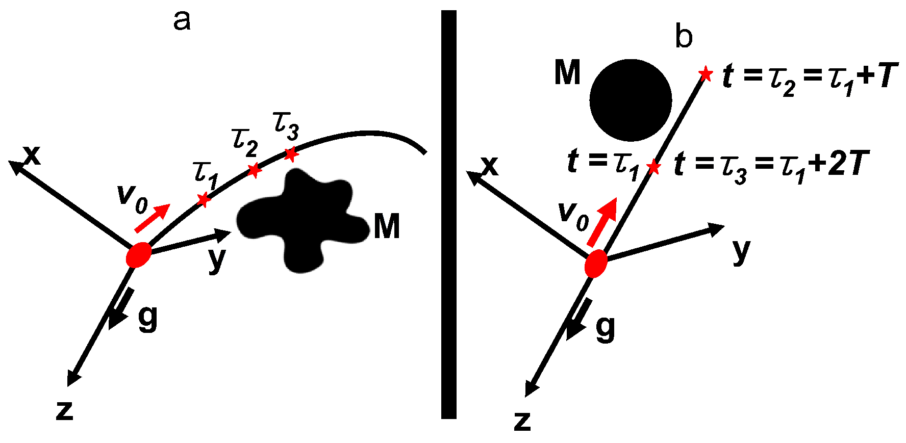
Schematic representation of an atom interferometer in the presence of a test mass M. The atom cloud of the interferometer is launched at with velocity and interacts with Raman pulses at times , and , indicated by the stars in the diagram. (a) A generic interferometer; (b) the fountain geometry used for the numerical calculations. In this case, the mass is a point mass or spherical mass having radius that is centered at position at time The case of a stationary test mass () and a test mass moving at constant velocity () are considered. The modification of the signal produced by the test mass would be a maximum if the atom cloud were to touch the test mass at the top of the cloud’s trajectory.
Figure 1.
Schematic representation of an atom interferometer in the presence of a test mass M. The atom cloud of the interferometer is launched at with velocity and interacts with Raman pulses at times , and , indicated by the stars in the diagram. (a) A generic interferometer; (b) the fountain geometry used for the numerical calculations. In this case, the mass is a point mass or spherical mass having radius that is centered at position at time The case of a stationary test mass () and a test mass moving at constant velocity () are considered. The modification of the signal produced by the test mass would be a maximum if the atom cloud were to touch the test mass at the top of the cloud’s trajectory.

Figure 2.
Stationary source. Plot , maximum of the phase magnitude given in Eqs. (62c) and (66) versus the impact parameter ; Plot , the same as Plot , but for ; Plot , dependence of the exact (black curve) and approximate (red curve) phases as a function of the initial z-coordinate () for , where the phase achieves its maximum magnitude; Plot , the same as Plot , but for , where the phase passes below the noise threshold ; Plots , the same as Plot , but for the maximum magnitude of the difference between exact and approximate phases given in Eqs. (62c), (66), (70) and (99a); Plot , the same as Plot , but for , where the magnitude of phase difference shown on Plot passes below ; Plot , the difference between black and red curves in Plot ; Plots , the same as Plots , but for the magnitude of the quantum correction given in Eqs. (62d) and (73); the values of are for and for , where the magnitude of the phase difference shown on Plot passes below ; exact quantum correction , approximations and are shown in black, red and blue, respectively. Plots , the same as Plots , but for the maximum magnitude of the difference between exact and approximate quantum corrections given in Eqs. (62d), (73), (75a) and (77); in Plot where the magnitude of the phase difference shown on Plot passes below Plots , the same as Plots , but for the maximum magnitude of the difference between exact and approximate quantum corrections given in Eqs. (62d), (73), (81) and (99b); in Plot , where the magnitude of the phase difference shown on Plot passes below . Plots , the same as Plots , but for the magnitude of the Q-term given in Eq. (91); values of are for and for , where the magnitude of the phase shown on Plot passes below Plots , the same as Plots , but for the maximum magnitude of the difference between exact and approximate Q-terms given in Eqs. (91), (94) and (99c); in Plot , where the magnitude of the difference shown on Plot passes below


Figure 3.
Test mass moving with constant velocity 5 m/s. Columns 1, 2 and 3 mirror Columns 1,3 and 4 of Figure 2. Values of are for Plots , , for Plot , for Plots for Plot for Plot for Plot for Plot for Plot and for Plot
Figure 3.
Test mass moving with constant velocity 5 m/s. Columns 1, 2 and 3 mirror Columns 1,3 and 4 of Figure 2. Values of are for Plots , , for Plot , for Plots for Plot for Plot for Plot for Plot for Plot and for Plot


| Earth’s gravitational field | |
| Multiple- beam splitter factor | |
| Effective wave vector | m |
| Time between launch and first Raman pulse | ms |
| Time between Raman pulses | ms |
| Launch velocity | |
| Error of atom interferometer phase measurement | rad |
| Test mass | kg |
| Atomic mass | 87 |
Table 2.
Locations of regions of validity of the exact and approximate expressions for the stationary and moving test mass. The regions refer to Regions 1–7 given in the text.
| Region | Stationary Test Mass | Test Mass Moving With Constant Velocity |
|---|---|---|
| 1 | m | m |
| 2 | m | m |
| 3 | m | m |
| 4 | m | m |
| 5 | m | m |
| 6 | m | m |
| 7 | m | m |
© 2016 by the authors; licensee MDPI, Basel, Switzerland. This article is an open access article distributed under the terms and conditions of the Creative Commons Attribution (CC-BY) license (http://creativecommons.org/licenses/by/4.0/).
Share and Cite
MDPI and ACS Style
Dubetsky, B.; Libby, S.B.; Berman, P. Atom Interferometry in the Presence of an External Test Mass. Atoms 2016, 4, 14. https://doi.org/10.3390/atoms4020014
AMA Style
Dubetsky B, Libby SB, Berman P. Atom Interferometry in the Presence of an External Test Mass. Atoms. 2016; 4(2):14. https://doi.org/10.3390/atoms4020014
Chicago/Turabian StyleDubetsky, Boris, Stephen B. Libby, and Paul Berman. 2016. "Atom Interferometry in the Presence of an External Test Mass" Atoms 4, no. 2: 14. https://doi.org/10.3390/atoms4020014
Note that from the first issue of 2016, this journal uses article numbers instead of page numbers. See further details here.