Influence of the p ¯ -p Nuclear Interaction on the Rate of the Low-Energy p ¯ + H μ → ( p ¯ p ) α + μ − Reaction

Abstract

The influence of an additional strong $\overline{\mathrm{p}}$-p nuclear interaction in a three-charge-particle system with arbitrary masses is investigated. Specifically, the system of $\overline{\mathrm{p}},{\mu }^{-}$, and p is considered in this paper, where $\overline{\mathrm{p}}$ is an antiproton, ${\mu }^{-}$ is a muon and p is a proton. A numerical computation in the framework of a detailed few-body approach is carried out for the following protonium (antiprotonic hydrogen) formation three-body reaction: $\overline{\mathrm{p}}+{\mathrm{H}}_{\mu }\left(1s\right)\to {\left(\overline{\mathrm{p}}\mathrm{p}\right)}_{\alpha }+{\mu }^{-}$. Here, ${\mathrm{H}}_{\mu }\left(1s\right)$ is a ground state muonic hydrogen, i.e., a bound state of p and ${\mu }^{-}$. A bound state of p and its antimatter counterpart $\overline{\mathrm{p}}$ is a protonium atom in a quantum atomic state $\alpha$, i.e., $Pn={\left(\overline{\mathrm{p}}\mathrm{p}\right)}_{\alpha }$. The low-energy cross sections and rates of the $Pn$ formation reaction are computed in the framework of coupled Faddeev-Hahn-type equations. The strong $\overline{\mathrm{p}}$-p interaction is included in these calculations within a first order approximation. It was found, that the inclusion of the nuclear interaction results in a quite significant correction to the rate of the three-body reaction.

1. Introduction

The first detection and exploration of antiprotons, $\overline{\mathrm{p}}$’s, [1] occurred more than a half of a century ago. Since that time this research field, which is related to stable baryonic particles, has seen substantial developments in both experimental and theoretical aspects. This field of particle physics represents one of the most important sections of such research work at CERN.

It will suffice to mention such experimental research groups as ALPHA [2], ATRAP [3], ASACUSA [4,5] and others, which carry out experiments with antiprotons. By using slow antiprotons it is then possible to create ground state antihydrogen atoms ${\overline{\mathrm{H}}}_{1s}$ (a bound state of $\overline{\mathrm{p}}$ and $e^{+}$, i.e., a positron) at low temperatures. The resulting two-particle atom at present can be viewed as one of the simplest and most stable anti-matter species [6]. A comparison of the properties of the resulting hydrogen atom H with $\overline{\mathrm{H}}$ reveals that this antiatom lends itself well to support testing of the fundamentals of physics [2]. Developments in regard to atomcules and $\overline{\mathrm{H}}$ atoms have increased interest in the protonium ($Pn$) atom as well. This atom can be viewed as a bound state of $\overline{\mathrm{p}}$ and p [7,8,9]. The two-heavy-charge-particle system can also be described as antiprotonic hydrogen. Its characteristics within the atomic scale are that it is a heavy and an extremely small system containing strong Coulomb and nuclear interactions. There is an interplay between these interactions inside the atom. This situation is responsible for the creation of interesting resonance and quasi-bound states in $Pn$ [10]. Thus, $Pn$ can be considered as a useful tool in the examination of the antinucleon-nucleon $\left(\overline{N}N\right)$ interaction potential [11,12,13,14] as well as the annihilation processes [15,16,17].

In other words, the interplay between Coulomb and nuclear forces contributes greatly to $\overline{\mathrm{p}}$ and p quantum dynamics [18]. Further, the $\overline{\mathrm{p}}+$p elastic scattering problem has also been examined in numerous papers. A good representative example would be paper [16]. It is also worthwhile to note that $Pn$ formation is related to charmonium-a hydrogen-like atom $\left(\overline{c}c\right)$, which is also known as a bound state of a c-antiquark $\left(\overline{c}\right)$ and c-quark [16]. In sum, the fundamental importance of protonium and problems related to its formation, i.e., bound or quasi-bound states, resonances and spectroscopy, have resulted in this two-particle atom gaining much attention in recent decades. Several few-charge-particle collisions can be used in order to produce low-energy $Pn$ atoms. The following reaction is, for instance, one of them:

$$\overline{\mathrm{p}}+\mathrm{H}\left(1s\right)\to {\left(\overline{\mathrm{p}}\mathrm{p}\right)}_{{\alpha }^{\prime }}+e^{-}.$$

(1)

This process is a Coulomb three-body collision which was computed in a few works in which different methods and techniques have been applied [19,20,21,22]. Because in this three-body process a heavy particle, i.e., a proton, is transferred from one negative “center”, $e^{-}$, to another, $\overline{\mathrm{p}}$, it would be difficult to apply a computational method based on an adiabatic (Born-Oppenheimer) approach [23]. Besides, experimentalists use another few-body reaction to produce $Pn$ atoms, i.e., a collision between a slow $\overline{\mathrm{p}}$ and a positively charged molecular hydrogen ion, i.e., H${}_2^{+}$:

$$\overline{\mathrm{p}}+{\mathrm{H}}_2^{+}\to {\left(\overline{\mathrm{p}}\mathrm{p}\right)}_{{\alpha }^{\prime }}+\mathrm{H}.$$

(2)

Nonetheless, this paper is devoted to another possible three-body process of the $Pn$ formation reaction in which we compute the cross-section and rate of a collision between $\overline{\mathrm{p}}$ and a muonic hydrogen atom H${}_{\mu }$, which is a bound state of p and a negative muon:

$$\overline{\mathrm{p}}+{\left(\mathrm{p}\mu \right)}_{1s}\to {\left(\overline{\mathrm{p}}\mathrm{p}\right)}_{\alpha }+{\mu }^{-}.$$

(3)

Here, $\alpha$ = $1s$, $2s$ or $2p$ is the final quantum atomic state of $Pn$. Since the participation of ${\mu }^{-}$ in (3), at low-energy collisions $Pn$ would be formed in a very small size—in the ground and close to ground states $\alpha$. It is obvious that in these states the hadronic nuclear force between $\overline{\mathrm{p}}$ and p will be strong and pronounced. In its ground state the $Pn$ atom has the following size: $a_0\left(Pn\right)={\hslash }^2/(e_0^2{m}_{\mathrm{p}}/2)\sim$ 50 fm, in which the Coulomb interaction between $\overline{\mathrm{p}}$ and p becomes extremely strong. The corresponding $Pn$’s binding energy without the inclusion of the nuclear $\overline{\mathrm{p}}$-p interaction is: $E_n\left(Pn\right)=-e_0^4{m}_{\mathrm{p}}/2/(2\hslash n^2)\sim -$10 keV. We take: $n=1$, ℏ is the Planck constant, $e_0$ is the electron charge, and $m_{\mathrm{p}}$ is the proton mass. Muons are already used as an effective tool to search for “new physics” and to carry out precise measurements of some fundamental constants [24]. For example, in the atomic analog of the reaction (3) $Pn$ would be formed at highly excited Rydberg states with ${\alpha }^{\prime }\approx 30$. Therefore, it is interesting to investigate the $\overline{\mathrm{p}}$-p nuclear interaction in the framework of the muonic three-body reaction (3) at low-energy collisions.

In this paper the reaction (3) is treated as a Coulomb three-body system (123) with arbitrary masses: $m_1,m_2$, and $m_3$. This is shown in Figure 1 and Figure 2. A few-body method based on a Faddeev-type equation formalism is used. In the next sections we will introduce notation pertinent to the few-body system (123), the basic equations, boundary conditions, and a brief derivation of the set of coupled one-dimensional integral-differential equations. The muonic atomic units (m.a.u. or m.u.) are used in this work, i.e., $e=\hslash =m_{\mu }=1$ and $m_{\mu }=206.769m_e$ is the mass of the muon, where $m_e$ is the electron mass. The proton (anti-proton) mass is $m_p=m_{\overline{p}}$ = 1836.152 $m_e$.

2. A Few-Body Approach

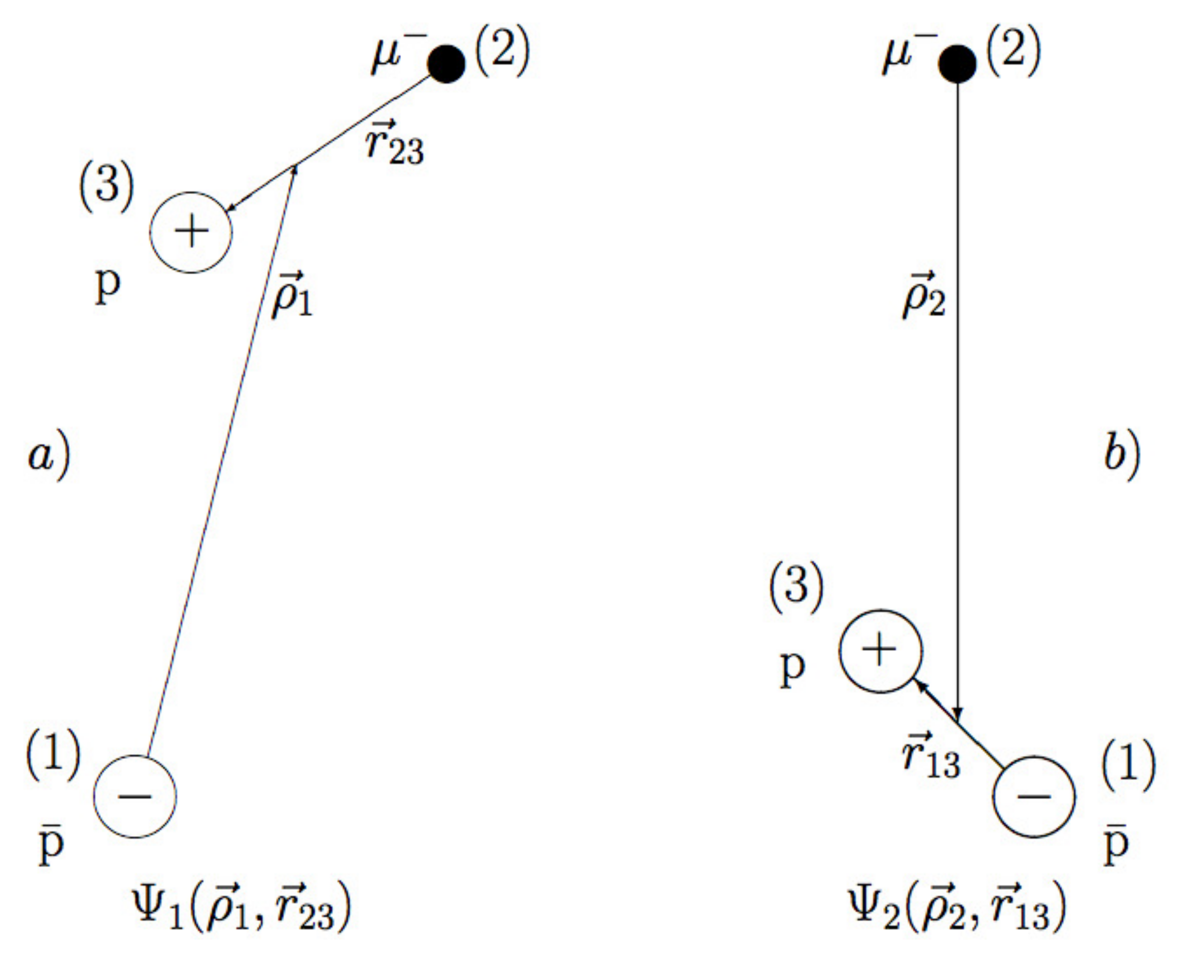
The main thrust of this paper is the three-body reaction (3). As we have already mentioned, a quantum-mechanical Faddeev-type few-body method is applied in this work. A coordinate space representation is used. In this approach the three-body wave function is decomposed into two independent Faddeev-type components [25]. Each component is determined by its own independent Jacobi coordinates. Since the reaction (3) is considered at low energies, i.e., well below the three-body break-up threshold, the Faddeev-type components are quadratically integrable over the internal target variables ${\overrightarrow{r}}_{23}$ and ${\overrightarrow{r}}_{13}$. They are shown in Figure 1 and Figure 2.

2.1. Coupled Integral-Differential Equations

In general, the Faddeev approach is based on a reduction of the total three-body wave function $\mathrm{\Psi }$ on three Faddeev-type components [25]. However, when one has two negative and one positive charges only two asymptotic configurations are possible below the system’s total energy $\left(E\right)$ break-up threshold. In the framework of an adiabatic hyperspherical close-coupling approach, the Coulomb three-body system has been considered in Ref. [26]. Nevertheless, one can also apply a few-body type method to the three-body system in which one can decompose $\mathrm{\Psi }$ on two components and devise a set of two coupled equations [27]. This is done in the current paper.

Additionally, it would be interesting to investigate and estimate the effect of the strong $\overline{\mathrm{p}}$-p nuclear interaction in the final state of the reaction (3). In this work, the nuclear $\overline{\mathrm{p}}$-p interaction is included approximately by shifting the Coulomb (atomic) energy levels in $Pn$. For a number of reasons the direct $\overline{\mathrm{p}}$-p annihilation channel in (3) is not included in the current calculations. This approximation is discussed at the end of this subsection. Next, a modified close coupling approach (MCCA) is applied in this work in order to solve the Faddeev-Hahn-type (FH-type) equations [28,29,30,31,32]. In other words, we carry out an expansion of the Faddeev-type components into eigenfunctions of the subsystem Hamiltonians [33,34]. This technique provides an infinite set of coupled one-dimensional integral-differential equations.

We denote an antiproton $\overline{\mathrm{p}}$ by 1, a negative muon ${\mu }^{-}$ by 2, and a proton p by 3, and use the following system of units: $e=\hslash =m_2=1$. The total Hamiltonian of the three-body system is:

$$\widehat{H}={\widehat{H}}_0+V_{12}\left({\overrightarrow{r}}_{12}\right)+V_{23}\left({\overrightarrow{r}}_{23}\right)+{\mathbb{V}}_{13}\left({\overrightarrow{r}}_{13}\right),$$

(4)

where ${\widehat{H}}_0$ is the total kinetic energy operator of the three-body system, $V_{12}\left({\overrightarrow{r}}_{12}\right)$ and $V_{23}\left({\overrightarrow{r}}_{23}\right)$ are Coulomb pair-interaction potentials between particles 12 and 23 respectively, and:

$${\mathbb{V}}_{13}\left({\overrightarrow{r}}_{13}\right)=V_{13}\left({\overrightarrow{r}}_{13}\right)+v_{13}^{\overline{N}N}\left({\overrightarrow{r}}_{13}\right)$$

(5)

is the Coulomb+nuclear interaction between particles 13, i.e., $\overline{\mathrm{p}}$ and p. $v_{13}^{\overline{N}N}\left({\overrightarrow{r}}_{13}\right)$ is the $\overline{N}N$ strong short-range interaction between the particles. The last potential is considered as an approximate spherical symmetric interaction in this work. The system is depicted in Figure 1 and Figure 2 together with the Jacobi coordinates $\{{\overrightarrow{r}}_{j3},{\overrightarrow{\rho }}_k\}$ and the different geometrical angles between the vectors:

$$\begin{array}{c}{\overrightarrow{r}}_{j3}={\overrightarrow{r}}_3-{\overrightarrow{r}}_j,\end{array}$$

(6)

$$\begin{array}{c}{\overrightarrow{\rho }}_k=\frac{(m_3{\overrightarrow{r}}_3+m_j{\overrightarrow{r}}_j)}{(m_3+m_j)}-{\overrightarrow{r}}_k,(j\ne k=1,2).\end{array}$$

(7)

Here ${\overrightarrow{r}}_{\xi }$, $m_{\xi }$ are the coordinates and the masses of the particles $\xi =1,2,3$ respectively. This circumstance suggests a few-body Faddeev formulation which uses only two components. A general procedure to derive such formulations is described in Ref. [27]. In this approach, the three-body wave function is represented as follows:

$$|\mathrm{\Psi }\rangle ={\mathrm{\Psi }}_1({\overrightarrow{r}}_{23},{\overrightarrow{\rho }}_1)+{\mathrm{\Psi }}_2({\overrightarrow{r}}_{13},{\overrightarrow{\rho }}_2),$$

(8)

where each Faddeev-type component is determined by its own Jacobi coordinates. Moreover, ${\mathrm{\Psi }}_1({\overrightarrow{r}}_{23},{\overrightarrow{\rho }}_1)$ is quadratically integrable over the variable ${\overrightarrow{r}}_{23}$, and ${\mathrm{\Psi }}_2({\overrightarrow{r}}_{13},{\overrightarrow{\rho }}_2)$ over the variable ${\overrightarrow{r}}_{13}$. To define $|{\mathrm{\Psi }}_l\rangle$, $(l=1,2)$ a set of two coupled Faddeev-Hahn-type equations would be:

$$\begin{array}{c}\left(E-{\widehat{H}}_0-V_{23}\left({\overrightarrow{r}}_{23}\right)\right){\mathrm{\Psi }}_1({\overrightarrow{r}}_{23},{\overrightarrow{\rho }}_1)=\left(V_{23}\left({\overrightarrow{r}}_{23}\right)+V_{12}\left({\overrightarrow{r}}_{12}\right)\right){\mathrm{\Psi }}_2({\overrightarrow{r}}_{13},{\overrightarrow{\rho }}_2),\end{array}$$

(9)

$$\begin{array}{c}\left(E-{\widehat{H}}_0-{\mathbb{V}}_{13}\left({\overrightarrow{r}}_{13}\right)\right){\mathrm{\Psi }}_2({\overrightarrow{r}}_{13},{\overrightarrow{\rho }}_2)=\left({\mathbb{V}}_{13}\left({\overrightarrow{r}}_{13}\right)+V_{12}\left({\overrightarrow{r}}_{12}\right)\right){\mathrm{\Psi }}_1({\overrightarrow{r}}_{23},{\overrightarrow{\rho }}_1).\end{array}$$

(10)

Here, ${\widehat{H}}_0$ is the kinetic energy operator of the three-particle system, $V_{ij}\left(r_{ij}\right)$ are paired Coulomb interaction potentials $(i\ne j=1,2,3)$, E is the total energy, and ${\mathbb{V}}_{13}\left({\overrightarrow{r}}_{13}\right)$ is represented in Equation (5). It is important to point out here that the constructed equations satisfy the Schrődinger equation exactly [27]. For the energies below the three-body break-up threshold, these equations exhibit the same advantages as the Faddeev equations [25], because they are formulated for the wave function components with correct physical asymptotes.

In addition, in the framework of these equations the two-particle atomic states, i.e., subsystems ($\mathrm{p}\mu$) and $\left(\overline{\mathrm{p}}\mathrm{p}\right)$, are considered in a similar way, and the Faddeev approach prevents the overcompleteness problem—two independent complete-basis expansion functions are used within a set of two coupled equations. Next, the kinetic energy operator ${\widehat{H}}_0$ in Equations (9) and (10) can be represented as: ${\widehat{H}}_0={\widehat{T}}_{{\rho }_i}+{\widehat{T}}_{r_{ij}}$, then one can re-write the Equations (9) and (10) in the following way:

$$\begin{array}{ccc}\hfill \left(E-{\widehat{T}}_{{\rho }_1}-{\widehat{h}}_{23}\left({\overrightarrow{r}}_{23}\right)\right){\mathrm{\Psi }}_1({\overrightarrow{r}}_{23},{\overrightarrow{\rho }}_1)& =& \left(V_{23}\left({\overrightarrow{r}}_{23}\right)+V_{12}\left({\overrightarrow{r}}_{12}\right)\right){\mathrm{\Psi }}_2({\overrightarrow{r}}_{13},{\overrightarrow{\rho }}_2),\hfill \end{array}$$

(11)

$$\begin{array}{ccc}\left(E-{\widehat{T}}_{{\rho }_2}-{\widehat{h}}_{13}^{\overline{N}N}\left({\overrightarrow{r}}_{13}\right)\right){\mathrm{\Psi }}_2({\overrightarrow{r}}_{13},{\overrightarrow{\rho }}_2)\hfill & =& \left(V_{13}\left({\overrightarrow{r}}_{13}\right)+v_{13}^{\overline{N}N}\left({\overrightarrow{r}}_{13}\right)+V_{12}\left({\overrightarrow{r}}_{12}\right)\right)\times {\mathrm{\Psi }}_1({\overrightarrow{r}}_{23},{\overrightarrow{\rho }}_1).\hfill \end{array}$$

(12)

The two-body target hamiltonians ${\widehat{h}}_{23}\left({\overrightarrow{r}}_{23}\right)={\widehat{T}}_{{\overrightarrow{r}}_{23}}+V_{23}\left({\overrightarrow{r}}_{23}\right)$ and ${\widehat{h}}_{13}^{\overline{N}N}\left({\overrightarrow{r}}_{13}\right)={\widehat{T}}_{{\overrightarrow{r}}_{13}}+V_{13}\left({\overrightarrow{r}}_{13}\right)+v_{13}^{\overline{N}N}\left({\overrightarrow{r}}_{13}\right)$ with an additional $\overline{\mathrm{p}}$-p nuclear interaction are represented explicitly in these equations. In order to solve Equations (11) and (12) a modified close-coupling approach is applied, which leads to an expansion of the system’s wave function components ${\mathrm{\Psi }}_1$ and ${\mathrm{\Psi }}_2$ into eigenfunctions ${\phi }_n^{\left(1\right)}\left({\overrightarrow{r}}_{23}\right)$ and ${\phi }_{n^{\prime }}^{\left(2\right)\overline{N}N}\left({\overrightarrow{r}}_{13}\right)$ of the subsystem (target) Hamiltonians:

$$\begin{array}{c}\hfill \left\{\begin{array}{c}{\mathrm{\Psi }}_1({\overrightarrow{r}}_{23},{\overrightarrow{\rho }}_1)\approx ({\displaystyle \int }+{\displaystyle \sum {)}_n}{f}_n^{\left(1\right)}\left({\overrightarrow{\rho }}_1\right){\phi }_n^{\left(1\right)}\left({\overrightarrow{r}}_{23}\right),\hfill \\ {\mathrm{\Psi }}_2({\overrightarrow{r}}_{13},{\overrightarrow{\rho }}_2)\approx ({\displaystyle \int }+{\displaystyle \sum {)}_{n^{\prime }}}{f}_{n^{\prime }}^{\left(2\right)}\left({\overrightarrow{\rho }}_2\right){\phi }_{n^{\prime }}^{\left(2\right)\overline{N}N}\left({\overrightarrow{r}}_{13}\right).\hfill \end{array}\right.\end{array}$$

(13)

This provides a set of coupled one-dimensional integral-differential equations after the partial-wave projection. The two complete sets of functions, i.e., $\{{\phi }_n^{\left(1\right)}\left({\overrightarrow{r}}_{23}\right)\}$ and $\{{\phi }_{n^{\prime }}^{\left(2\right)\overline{N}N}\left({\overrightarrow{r}}_{13}\right)\}$, represent the eigenfunctions of the two-body target hamiltonians ${\widehat{h}}_{23}\left({\overrightarrow{r}}_{23}\right)$ and ${\widehat{h}}_{13}^{\overline{N}N}\left({\overrightarrow{r}}_{13}\right)$ respectively:

$$\begin{array}{ccc}\hfill {\widehat{h}}_{23}\left({\overrightarrow{r}}_{23}\right){\phi }_n^{\left(1\right)}\left({\overrightarrow{r}}_{23}\right)& =& \left[{\widehat{T}}_{{\overrightarrow{r}}_{23}}+V_{23}\left({\overrightarrow{r}}_{23}\right)\right]{\phi }_n^{\left(1\right)}\left({\overrightarrow{r}}_{23}\right)={\epsilon }_n{\phi }_n^{\left(1\right)}\left({\overrightarrow{r}}_{23}\right)\hfill \end{array}$$

(14)

$$\begin{array}{ccc}\hfill {\widehat{h}}_{13}^{\overline{N}N}\left({\overrightarrow{r}}_{13}\right){\phi }_{n^{\prime }}^{\left(2\right)\overline{N}N}\left({\overrightarrow{r}}_{13}\right)& =& \left[{\widehat{T}}_{{\overrightarrow{r}}_{13}}+V_{13}\left({\overrightarrow{r}}_{13}\right)+v_{13}^{\overline{N}N}\left({\overrightarrow{r}}_{13}\right)\right]{\phi }_{n^{\prime }}^{\left(2\right)\overline{N}N}\left({\overrightarrow{r}}_{13}\right)={\mathcal{E}}_{n^{\prime }}{\phi }_{n^{\prime }}^{\left(2\right)\overline{N}N}\left({\overrightarrow{r}}_{13}\right)\hfill \end{array}$$

(15)

In addition to the Coulomb potential, the strong interaction, $v_{13}^{\overline{N}N}\left({\overrightarrow{r}}_{13}\right)$, is also included in Equation (15). Coulomb is a central symmetric potential. Therefore, the eigenfunctions ${\phi }_n^{\left(1\right)}$ and the corresponding eigenstates are [35]:

$$\begin{array}{c}{\phi }_n^{\left(1\right)}\left({\overrightarrow{r}}_{23}\right)={\sum }_{lm}{R}_{nl}^{\left(1\right)}\left(r_{23}\right)Y_{lm}\left({\overrightarrow{r}}_{23}\right),\end{array}$$

(16)

$$\begin{array}{c}{\epsilon }_n=-\frac{{\mu }_1}{2n^2}.\end{array}$$

(17)

The full potential between $\overline{\mathrm{p}}$ and p is more complex, because its second part, $v_{13}^{\overline{N}N}\left({\overrightarrow{r}}_{13}\right)$, possesses an asymmetric $\overline{N}N$ nuclear interaction [16,17]. We did not explicitly include the strong interaction in the current calculations. Therefore, in the case of the target $Pn$ eigenfunctions we used the two-body pure Coulomb (atomic) wave functions. Nonetheless, the strong $\overline{\mathrm{p}}$-p interaction is approximately taken into account in this work through the eigenstates ${\mathcal{E}}_{n^{\prime }}$ which have shifted values from the original Coulomb levels ${\epsilon }_{n^{\prime }}$ [36], that is:

$$\begin{array}{c}{\phi }_{n^{\prime }}^{\left(2\right)\overline{N}N}\left({\overrightarrow{r}}_{13}\right)\approx {\sum }_{l^{\prime }{m}^{\prime }}{R}_{n^{\prime }{l}^{\prime }}^{\left(2\right)\overline{N}N}\left(r_{13}\right)Y_{l^{\prime }{m}^{\prime }}\left({\overrightarrow{r}}_{13}\right)\approx {\sum }_{l^{\prime }{m}^{\prime }}{R}_{n^{\prime }{l}^{\prime }}^{\left(2\right)}\left(r_{13}\right)Y_{l^{\prime }{m}^{\prime }}\left({\overrightarrow{r}}_{13}\right)\end{array}$$

(18)

$$\begin{array}{c}{\mathcal{E}}_{n^{\prime }}\approx {\epsilon }_{n^{\prime }}+\Delta E_{n^{\prime }}^{\overline{N}N}=-\frac{{\mu }_2}{2n^{\prime 2}}+\Delta E_{n^{\prime }}^{\overline{N}N}.\end{array}$$

(19)

In Equations (16) and (18) $Y_{lm}\left(\overrightarrow{r}\right)$ are spherical functions [35] and $R_{nl}^{\left(i\right)}\left(r\right)$ $(i=1,2)$ is an analytical solution to the radial part of the two-charge-particle Schrődinger equation [35]. The method outlined above is a first order approximation. In the framework of this approach it would be interesting to estimate the level of influence of the strong $\overline{\mathrm{p}}$-p interaction on the three-charge-particle proton transfer reaction (3). Broadly speaking, the two-body Coulomb-nuclear wave functions of $Pn$, i.e., ${\phi }_{n^{\prime }}^{\left(2\right)\overline{N}N}\left({\overrightarrow{r}}_{13}\right)$ and corresponding eigenstates, ${\mathcal{E}}_{n^{\prime }}$, have been of a significant interest for a long time. To build these states one needs to solve the two-charge-particle Schrődinger equation with an additional strong short-range $\overline{N}N$ interaction, i.e., Equation (15), see for instance [14]. In Ref. [37] the authors explicitly included the nuclear $\overline{\mathrm{p}}$-p interaction in the framework of a variational approach for the case of an $\overline{\mathrm{H}}$ + H scattering problem. However, as a first step, one can also apply an approximate approach (Equations (16)–(18)) with an energy shift in the eigenstate of $Pn$ ${\mathcal{E}}_{n^{\prime }}$, i.e., Equation (19), ${\epsilon }_{n^{\prime }}$ is the Coulomb level and $\Delta E_{n^{\prime }}^{\overline{N}N}$ is its nuclear shift. It can be computed, for example, with the use of the following formula [36]:

$$\Delta E_{n^{\prime }}^{\overline{N}N}=-\frac{4}{n^{\prime }}\frac{a_s}{B_{Pn}}{\epsilon }_{n^{\prime }},$$

(20)

where $a_s$ is the strong interaction scattering length in the $\overline{\mathrm{p}}$ + p collision, i.e., without inclusion of the Coulomb interaction between the particles, $B_{Pn}$ is the Bohr radius of $Pn$. In the literature one can find other approximate expressions to compute $\Delta E_{n^{\prime }}^{\overline{N}N}$, see for example [38,39]. It would also be interesting to apply some of these formulas in conjunction with the relativistic effects in protonium, see for example works [40].

After determining a proper angular momentum expansion one can obtain an infinite set of coupled integral-differential equations for the unknown functions $f_{\alpha }^{\left(1\right)}\left({\rho }_1\right)$ and $f_{{\alpha }^{\prime }}^{\left(2\right)}\left({\rho }_2\right)$ [29]:

$$\begin{array}{c}\hfill \left[{\left(k_n^{\left(1\right)}\right)}^2+\frac{{\partial }^2}{\partial {\rho }_1^2}-\frac{\lambda (\lambda +1)}{{\rho }_1^2}\right]f_{\alpha }^{\left(1\right)}\left({\rho }_1\right)=g_1\sum _{{\alpha }^{\prime }}\frac{\sqrt{(2\lambda +1)(2{\lambda }^{\prime }+1)}}{2L+1}\\ \hfill \times {\int }_0^{\infty }d{\rho }_2{f}_{{\alpha }^{\prime }}^{\left(2\right)}\left({\rho }_2\right){\int }_0^{\pi }d\omega sin\omega R_{nl}^{\left(1\right)}\left(\right|{\overrightarrow{r}}_{23}\left|\right)\left[-\frac{1}{|{\overrightarrow{r}}_{23}|}+\frac{1}{|{\overrightarrow{r}}_{12}|}\right]R_{n^{\prime }{l}^{\prime }}^{\left(2\right)}\left(\right|{\overrightarrow{r}}_{13}\left|\right)\\ \hfill \times {\rho }_1{\rho }_2\sum _{m{m}^{\prime }}{D}_{m{m}^{\prime }}^L(0,\omega ,0)C_{\lambda 0lm}^{Lm}{C}_{{\lambda }^{\prime }0l^{\prime }{m}^{\prime }}^{L{m}^{\prime }}{Y}_{lm}({\nu }_1,\pi )Y_{l^{\prime }{m}^{\prime }}^{*}({\nu }_2,\pi ),\end{array}$$

(21)

$$\begin{array}{c}\hfill \left[{\left(k_n^{\left(2\right)}\right)}^2+\frac{{\partial }^2}{\partial {\rho }_2^2}-\frac{{\lambda }^{\prime }({\lambda }^{\prime }+1)}{{\rho }_2^2}\right]f_{\alpha }^{\left(2\right)}\left({\rho }_2\right)=g_2\sum _{{\alpha }^{\prime }}\frac{\sqrt{(2\lambda +1)(2{\lambda }^{\prime }+1)}}{2L+1}\\ \hfill \times {\int }_0^{\infty }d{\rho }_1{f}_{{\alpha }^{\prime }}^{\left(1\right)}\left({\rho }_1\right){\int }_0^{\pi }d\omega sin\omega R_{nl}^{\left(2\right)}\left(\right|{\overrightarrow{r}}_{13}\left|\right)\left[-\frac{1}{|{\overrightarrow{r}}_{13}|}+\frac{1}{|{\overrightarrow{r}}_{12}|}\right]R_{n^{\prime }{l}^{\prime }}^{\left(1\right)}\left(\right|{\overrightarrow{r}}_{23}\left|\right)\\ \hfill \times {\rho }_2{\rho }_1\sum _{m{m}^{\prime }}{D}_{m{m}^{\prime }}^L(0,\omega ,0)C_{\lambda 0lm}^{Lm}{C}_{{\lambda }^{\prime }0l^{\prime }{m}^{\prime }}^{L{m}^{\prime }}{Y}_{lm}({\nu }_2,\pi )Y_{l^{\prime }{m}^{\prime }}^{*}({\nu }_1,\pi ).\end{array}$$

(22)

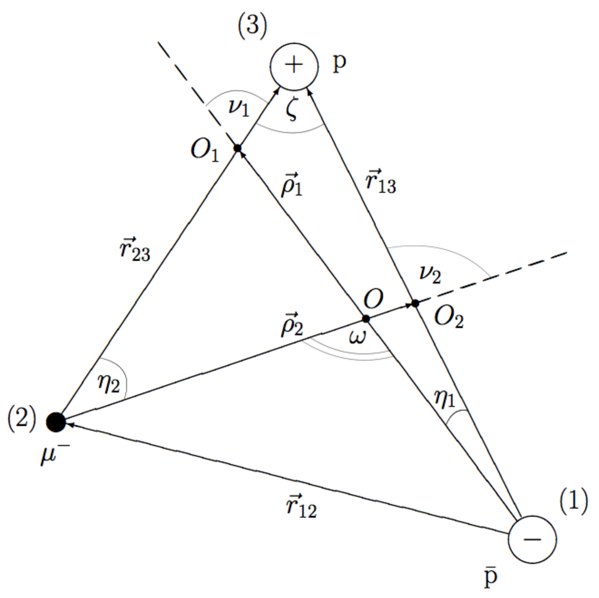
Here, $g_i=4\pi M_i/{\gamma }^3$ $(i=1,2)$, L is the total angular momentum of the three-body system, $\alpha =\left(nl\lambda \right)$ are quantum numbers of a three-body state, $k_n^{\left(i\right)}=\sqrt{2M_i(E-E_n^{\left(j\right)})}$, with $M_1=(m_2+m_3)m_1/(m_1+m_2+m_3)$, $M_2=(m_1+m_3)m_2/(m_1+m_2+m_3)$, $E_n^{\left(j\right)}$ is the binding energy of $\left(j3\right)$, $(i\ne j=1,2)$, $\gamma =1-m_1{m}_2/\left((m_1+m_3)(m_2+m_3)\right)$, $D_{m{m}^{\prime }}^L(0,\omega ,0)$ is the Wigner function [35], $C_{\lambda 0lm}^{Lm}$ is the Clebsh-Gordon coefficient [35], $\omega$ is the angle between the Jacobi coordinates ${\overrightarrow{\rho }}_i$ and ${\overrightarrow{\rho }}_{i^{\prime }}$, ${\nu }_i$ is the angle between ${\overrightarrow{r}}_{i^{\prime }3}$ and ${\overrightarrow{\rho }}_i$, ${\nu }_{i^{\prime }}$ is the angle between ${\overrightarrow{r}}_{i3}$ and ${\overrightarrow{\rho }}_{i^{\prime }}$. The following relationships are used for the numerical calculations: $sin{\nu }_i=({\rho }_{i^{\prime }}sin\omega )/\left(\gamma r_{i^{\prime }3}\right),cos{\nu }_i=({\beta }_i{\rho }_i+{\rho }_{i^{\prime }}cos\omega )\left(\gamma r_{i^{\prime }3}\right)$, where $(i\ne i^{\prime }=1,2).$ A detailed few-body treatment of the heavy-charge-particle reaction (3) is the main goal of this work. The geometric angles of the configurational triangle Δ123: ${\nu }_{1\left(2\right)}$, ${\eta }_{1\left(2\right)}$, $\zeta$, and $\omega$ are shown in Figure 2 together with the Jacobi coordinates, i.e., $\{{\overrightarrow{r}}_{j3},{\overrightarrow{\rho }}_k\}$ $(j\ne k=1,2)$ and ${\overrightarrow{r}}_{12}$. The center of mass of the (123) system is O. $O_1$ and $O_2$ are the center of masses of the targets. The Faddeev decomposition avoids over-completeness problems because the subsystems are treated in an equivalent way in the framework of the two-coupled equations.

In the framework of the first order approximation approach, the direct $\overline{\mathrm{p}}$-p annihilation channel in the reaction (3) is not included in this work. In the input channel of the reaction (3), $\overline{\mathrm{p}}$ + (p${}^{+}{\mu }^{-}{)}_{1s}$, the relatively heavy muon very effectively screens the strong Coulomb potential of the proton, and therefore it significantly prevents direct annihilation in (3) before the $Pn$ formation. In other words, the $Pn$ formation process dominates. However, it is another matter in the case of the atomic version of the $Pn$ formation reaction (1). Here, the electron cloud around the proton can also block the $\overline{\mathrm{p}}$ movement to p, but because of the quantum-tunneling effect the massive antiproton can penetrate with a significant probability through the light electron cloud and then directly annihilate with proton before protonium forms. Therefore, in the framework of the reaction (1) it would be necessary to take into account the tunneling effect. As far as we know, this is still not done in a suitable way.

In terms of the $Pn$ annihilation in the reaction (3) (which can occur after the two-body system formation) and an inclusion of this effect in calculations, it was mentioned above that in this case one needs to build precise Coulomb-nuclear $\overline{\mathrm{p}}$-p two-body wave functions ${\phi }_{n^{\prime }}^{\left(2\right)\overline{N}N}\left({\overrightarrow{r}}_{13}\right)$ from Equation (15). In this special case, one needs to consider not only the shifts of the Coulomb levels in Equation (19), but also their widths. However, in the current work, as a first order approximation the nuclear effect is considered only through Equations (19) and (20).

We believe that to some extent this approximation is justified. In this work, we were mostly interested in the $Pn$ atom formation process (3), where the values of the Coulomb-nuclear atomic levels at which the atom can form are important. As we mentioned, these levels have widths, but they are mostly responsible for the annihilation reaction that follows.

2.2. Boundary Conditions and Reaction cross Section

In order to reach the next step it is necessary to obtain a unique solution for Equations (21) and (22). While doing so it is important that the appropriate boundary conditions are chosen. They should be related to the physical situation of the system. In this paper we apply the same boundary conditions as in our previous papers [29,30]. In order to compute the cross sections we use the K-matrix formalism. This would appear to be a prudent step because this method has been successfully used to obtain solutions in various three-body problems within the framework of both the Schrődinger equation [41] and the coordinate space Faddeev equation [42,43]. Specifically, in regard to the rearrangement scattering problem $i+\left(j3\right)$ as the initial state within the asymptotic region it will be necessary to devise two solutions to Equations (21) and (22) which then will satisfy the boundary conditions that follow:

$$\begin{array}{c}\hfill \left\{\begin{array}{c}{f}_{nl}^{(i)}({\rho }_i)\underset{{\rho }_i\to 0}{\sim }0\hfill \\ f_{1s}^{(i)}({\rho }_i)\underset{{\rho }_i\to +\infty }{\sim }sin(k_1^{(i)}{\rho }_i)+K_{ii}cos(k_1^{(i)}{\rho }_i)\hfill \\ f_{1s}^{(j)}({\rho }_j)\underset{{\rho }_j\to +\infty }{\sim }\sqrt{v_i/v_j}{K}_{ij}cos(k_1^{(j)}{\rho }_j),\hfill \end{array}\right.\end{array}$$

(23)

where ${\mathit{K}}_{\mathit{ij}}$ represents the appropriate scattering coefficients, and $v_{i\left(j\right)}$ ($i\ne j=1,2$) is the $i\left(j\right)$ channel velocity between the particles. Next, one can use the following change of variables in Equations (21) and (22), i.e., ${\mathsf{f}}_{1s}^{\left(i\right)}\left({\rho }_i\right)=f_{1s}^{\left(i\right)}\left({\rho }_i\right)-sin(k_1^{\left(i\right)}{\rho }_i),(i=1,2).$ This substitution results in a modification of the variables and provides two sets of inhomogeneous equations which can now be conveniently solved numerically. The transition also allows the coefficients $K_{ij}$ to be gained by reaching a numerical solution for the previously described FH-type equations. The reaction cross section can be expressed as follows:

$${\sigma }_{ij}=\frac{4\pi }{k_1^{\left(i\right)2}}{\left|\frac{\mathbf{K}}{1-i\mathbf{K}}\right|}^2=\frac{4\pi }{k_1^{\left(i\right)2}}\frac{{\delta }_{ij}{D}^2+{\mathit{K}}_{ij}^2}{{(D-1)}^2+{({\mathit{K}}_{11}+{\mathit{K}}_{22})}^2},$$

(24)

where ($i,j=1,2$) refer to the two channels and $D=K_{11}{K}_{22}-K_{12}{K}_{21}$. Next, in accord with the quantum-mechanical unitarity principle the scattering matrix $\mathbf{K}=\left(\begin{array}{cc}{K}_{11}& K_{12}\\ K_{21}& K_{22}\end{array}\right)$ has an important feature: $K_{12}=K_{21}$, i.e., $\chi \left(E\right)=K_{12}/K_{21}=1$. The last equation has been checked for all considered collision energies within the framework of the 1s, 1s + 2s and 1s + 2s + 2p MCCA approximations, i.e., Equations (13).

3. Results and Conclusions

Below in this section we report our computational results. First of all, before attempting large scale production calculations one needs to investigate numerical convergence of the method and the computer program. It was very carefully undertaken in this work. The $Pn$ formation three-body reaction is computed at low energies. A Faddeev-like equation formalism Equations (11) and (12) has been applied. The few-body approach has been explained in previous sections. In order to solve the coupled equations, two different independent sets of target expansion functions have been employed (13). The goal of this paper is to carry out a reliable quantum-mechanical computation of the cross sections and corresponding rates of the $Pn$ formation reaction at low and very low collision energies. It is very interesting to estimate the influence of the strong short-range finale state $\overline{\mathrm{p}}$-p interaction on the rate of the reaction (3).

The three-body reaction (3) could, probably, be used to investigate the strong $\overline{\mathrm{p}}$-p nuclear potential and the annihilation process in future experiments with the anti-protonic hydrogen atom or protonium $Pn$. The coupled integral-differential Equations (21) have been solved numerically for the case of the total angular momentum $L=0$ in the framework of the two-level 2 × (1s), four-level 2 × (1s + 2s), and six-level 2 × (1s + 2s + 2p) close coupling approximations in Equation (13). The sign “2×” indicates that two different sets of expansion functions are applied. The $L=0$ computation is justified, because we are interested in a very low-energy collision: ${\epsilon }_{coll}\sim {10}^{-4}$ eV−10 eV. The following boundary conditions (23) have been applied. To compute the charge transfer cross sections the expression (24) has been used.

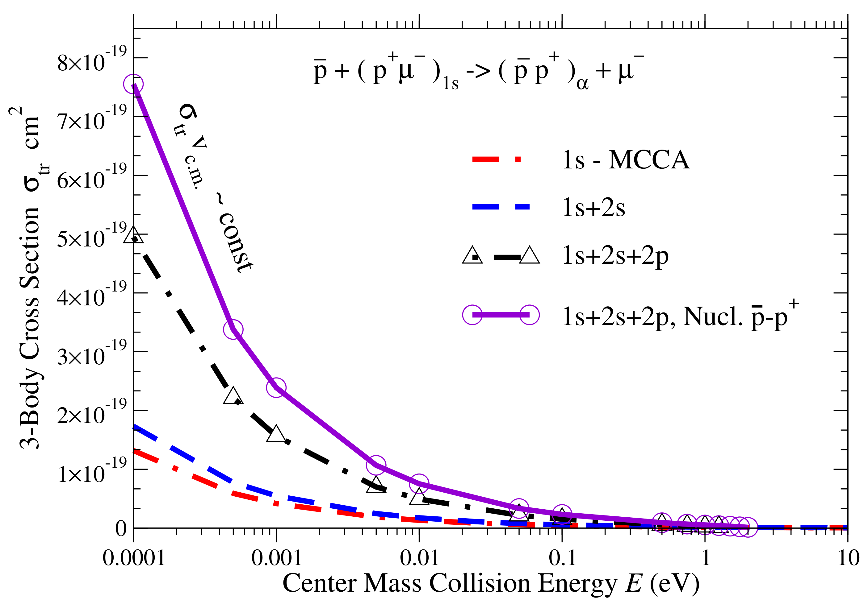
Because we compared the $Pn$ formation rates, ${\sigma }_{tr}{v}_{c.m.}$, of the process (3) with the corresponding results from Ref. [26], we also multiplied our data by factor of “$\times 5$”, as was done in [26]. We compared some of our findings with the corresponding data from the older work [26]. The $Pn$ formation cross section in the reaction (3) are shown in Figure 3. Here we use $1s$, $1s+2s$ and $1s+2s+2p$ states within the modified close-coupling approximation, i.e., MCCA approach. One can see that the contribution of the $2s$- and $2p$-states from each target is becoming even more significant while the collision energy becomes smaller. This is a well known fact that the $2p$-atomic-states are mostly responsible for the polarization effects in few-charge-particle systems. Our result from Figure 3 clearly depicts that this effect is becoming more important at low energy collisions.

It would also be useful to make a comment about the behavior of ${\sigma }_{tr}\left({\epsilon }_{coll}\right)$ at very low collision energies: ${\epsilon }_{coll}\sim 0$. From our calculations we found the following relationship in the proton transfer cross sections: ${\sigma }_{tr}\to \infty$ as ${\epsilon }_{coll}\to 0$. However, the proton transfer rates, ${\lambda }_{tr}$, are proportional to the product ${\sigma }_{tr}{v}_{c.m.}$ and this trends to a finite value as $v_{c.m.}\to 0$.

To compute the proton transfer rate the following formula ${\lambda }_{tr}={\sigma }_{tr}({\epsilon }_{coll}\to 0)v_{c.m.}$ can be used. Therefore, for process (3) we can compute the numerical value of the following important quantity: $\Lambda \left(Pn\right)={\sigma }_{tr}({\epsilon }_{coll}\to 0)v_{c.m.}\approx const$, which is proportional to the actual $Pn$ formation rate at low collision energies. In the framework of the $2\times (1s+2s+2p)$ MCCA approach, i.e., when six coupled Faddeev-Hahn-type integral-differential equations are solved, our result for the $Pn$ formation rate has the following value: ${\Lambda }_{1s2s2p}\left(Pn\right)\approx 0.32\mathrm{m}.\mathrm{a}.\mathrm{u}.$ The corresponding rate from work [26] is: ${\Lambda }^{\prime }\left(Pn\right)\approx 0.2$ m.a.u. Both of these results are in agreement with each other. For comparison purposes, our original result for ${\Lambda }_{1s2s2\mathrm{p}}\left(Pn\right)$ has been multiplied by a factor of “$\times 5$” to match work [26]. The unitarity relationship, i.e., $\chi \left(E\right)=K_{12}/K_{21}=1$, has been checked for different values of collision energies. It was shown, that $\chi$ always exhibits fairly constant values close to one. One of the main goals of this work is to investigate the effect of the $\overline{\mathrm{p}}$-p nuclear interaction on the rate of the reaction (3). In Figure 3 we additionally provide our cross sections for (3) including the nuclear effect in the final $Pn$ state. One can see, that the contribution of the strong interaction becomes even more substantial when the collision energy becomes lower. A few additional comments about the inclusion of the $\overline{\mathrm{p}}$-p nuclear interaction are appropriate. First of all, we neglected the $\overline{\mathrm{p}}$+p annihilation channel. This approximation has been discussed above. However, the effect of the strong nuclear forces on the reaction (3) is incorporated through the energy shifts $\Delta E_{n^{\prime }}^{\overline{N}N}$ to the original Coulomb energy levels in the $Pn$ atom, i.e., ${\epsilon }_{n^{\prime }}$ in Equation (19). To compute $\Delta E_{n^{\prime }}^{\overline{N}N}$ the expression (20) is used from [36]. The $\overline{\mathrm{p}}+$p elastic scattering length, i.e parameter $a_s$, was adopted from work [12] and equals 0.57 fm in our calculations. In [12] the Kohno-Weise strong interaction potential [44] has been applied. The next two Figure 4 and Figure 5 represent results in which we compare cross sections and rates computed with and without the inclusion of the strong potential within the different close-coupling approximation.

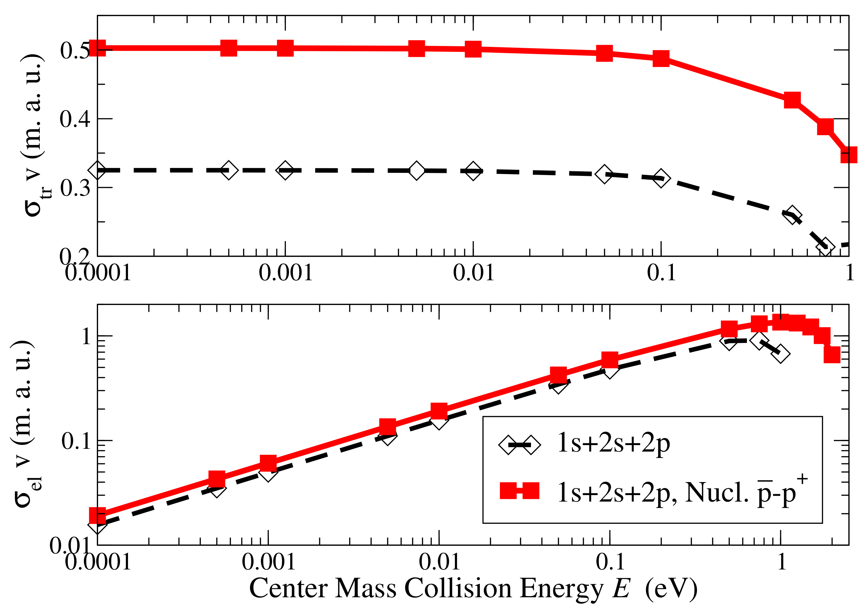
Figure 4 shows our results in the framework of the $1s$ and $1s+2s$ MCCA approaches. The results are numerically stable. It is seen that the contribution of the strong nuclear interaction is higher in the case of the $1s+2s$ approximation. For example, in this case the rate of the reaction (3) is about 0.12 m.a.u., however, with the inclusion of the nuclear interaction it becomes 0.15 m.a.u. The last figure in this paper, Figure 5, represents our computational data in the $1s+2s+2p$ approach. The very important polarization effect is included. The inclusion of the nuclear interaction brings a significant change to the rate of the reaction (3). At very low collision energies around ${10}^{-4}-{10}^{-2}$ eV, the rate is ∼0.5 m.a.u. It is important to restate that all calculations carried out in this work have been done for the ground-to-ground state of (3), i.e., $\alpha =1$.

In summation: the complexity of the few-body system and the method utilized necessitated that only the total orbital momentum $L=0$ be taken into account. However, the method was indeed adequate for the slow and ultraslow collisions discussed previously. Further, it is important to note that the devised few-body Equations (9) and (10) do exactly satisfy the Schrődinger equation. In cases in which the energies below the three-body break-up threshold occur, this methodology provides advantages similar to the Faddeev equations [25]. This is because these equations are formulated to include wave function components which contain the correct physical asymptotes. The solution of these equations begins by using a close-coupling approach. This then leads to an expansion of the system’s wave function components into eigenfunctions of the subsystem (target) Hamiltonians, which results in a set of one-dimensional integral-differential equations upon completion of the partial-wave projection. In an effort to expand the scope of the results a strong proton-antiproton interaction was included by appropriately shifting the Coulomb energy levels of the $Pn$ atom [14,36]. Interestingly, this process increased the magnitude of the resulting values of the reaction cross section and corresponding rate by ∼50%. Therefore, one further three-body reaction similar to (3) can also be of sufficient future interest:

$$\overline{\mathrm{p}}+{}^2{\mathrm{H}}_{\mu }\left(1s\right)\to {\left(\overline{\mathrm{p}}\mathrm{d}\right)}_{\alpha }+{\mu }^{-},$$

(25)

where ${}^2$H = d is the deuterium nucleus, ${\mu }^{-}$ and $\overline{\mathrm{p}}$ are muon and antiproton respectively. This is because of a possible effect of the isotopic few-body quantum dynamic differences between reactions (3) and (25), and the nuclear interaction differences between $\overline{\mathrm{p}}$ and p and $\overline{\mathrm{p}}$ and d. In the future, it would be very interesting to compare the cross sections of both reactions. Based on the results herein it seems logical for future work to include in Equations (13) the higher atomic target states as well as the continuum spectrum. Calculations of this type would be very interesting but challenging. The challenge is because at very low energy collisions the higher energy channels are closed and there is a significant energy gap between the states and the actual collision energies. Despite this limitation the primary contribution from s- and p-states (polarization) is still evaluated. In closing, the authors feel that including the strong $\overline{\mathrm{p}}$-p interaction explicitly in the numerical solution of Equations (11) and (12) could also provide an interesting and challenging direction for future theoretical research in this area.

References

- Chamberlain, O.; Segré, E.; Wiegand, C.; Ypsilantis, T. Observation of Antiprotons. Phys. Rev. 1955, 100, 947. [Google Scholar] [CrossRef]
- Ahmadi, M.; Alves, B.X.; Baker, C.J.; Bertsche, W.; Butler, E.; Capra, A.; Carruth, C.; Cesar, C.L.; Charlton, M.; Cohen, S.; et al. Observation of the 1S–2S transition in trapped antihydrogen. Nature 2017, 541, 506–510. [Google Scholar] [CrossRef] [PubMed]
- Gabrielse, G.; Kalra, R.; Kolthammer, W.S.; McConnell, R.; Richerme, P.; Grzonka, D.; Oelert, W.; Sefzick, T.; Zielinski, M.; Fitzakerley, D.W.; (ATRAP Collaboration). Trapped Antihydrogen in Its Ground State. Phys. Rev. Lett. 2012, 108, 113002. [Google Scholar] [CrossRef] [PubMed]
- Hori, M.; Hossein, A.-K.; Anna, S.; Daniel, B.; Andreas, D.; Ryugo, H. Takumi Kobayashi Buffer-gas cooling of antiprotonic helium to 1.5 to 1.7 K, and antiproton-to-electron mass ratio. Science 2016, 354, 610–614. [Google Scholar] [CrossRef] [PubMed]
- Kuroda, N.; Ulmer, S.; Murtagh, D.J.; Van, G.S.; Nagata, Y.; Diermaier, M.; Federmann, S.; Leali, M.; Malbrunot, C.; Mascagna, V.; et al. A source of antihydrogen for in-flight hyperfine spectroscopy. Nat. Commun. 2014, 5, 3089. [Google Scholar] [CrossRef] [PubMed]
- Amoretti, M.; Amsler, C.; Bonomi, G.; Bouchta, A.; Bowe, P.; Carraro, C.; Cesar, C.L.; Charlton, M.; Collier, M.J.T.; Doser, M.; et al. Production and detection of cold antihydrogen atoms. Nature 2002, 419, 456–459. [Google Scholar] [CrossRef] [PubMed]
- Zurlo, N.; ATHENA Collaboration. Evidence for the production of slow antiprotonic hydrogen in vacuum. Phys. Rev. Lett. 2006, 97, 153401. [Google Scholar] [CrossRef] [PubMed]
- Venturelli, L.; Amoretti, M.; Amsler, C.; Bonomi, G.; Carraroc, C.; Cesar, C.L.; Charlton, M.; Doser, M.; Fontana, A.; Funakosh, R.; et al. Protonium production in ATHENA. Nucl. Instrum. Methods Phys. Res. Sect. B 2007, 261, 40–43. [Google Scholar] [CrossRef]
- Rizzini, E.; Venturelli, L.; Zurlo, N.; Charlton, M.; Amsler, C.; Bonomi, G.; Canali, C.; Carraro, C.; Fontana, A.; Genova, P.; et al. Further evidence for low-energy protonium production in vacuum. Eur. Phys. J. Plus 2012, 127, 124. [Google Scholar] [CrossRef]
- Shapiro, I.S. The physics of nucleon-antinucleon systems. Phys. Rep. 1978, 35, 129–185. [Google Scholar] [CrossRef]
- Hrtánková, J.; Mareš, J. Interaction of antiprotons with nuclei. Nucl. Phys. A 2016, 945, 197–215. [Google Scholar]
- Carbonell, J.; Richard, J.-M.; Wycech, S. On the relation between protonium level shifts and nucleon-antinucleon scattering amplitudes. Z. Phys. A 1992, 343, 325–329. [Google Scholar] [CrossRef]
- Dover, C.B.; Richard, J.M. Spin observables in low energy nucleon-antinucleon scattering. Phys. Rev. C 1982, 25, 1952. [Google Scholar] [CrossRef]
- Richard, J.M.; Sainio, M.E. Nuclear effects in protonium. Phys. Lett. B 1982, 110, 349–352. [Google Scholar] [CrossRef]
- Desai, B.R. Proton-Antiproton Annihilation in Protonium. Phys. Rev. 1960, 119, 1385. [Google Scholar] [CrossRef]
- Klempt, E.; Bradamante, F.; Martin, A.; Richard, J.M. Antinucleon nucleon interaction at low energy: Scattering and protonium. Phys. Rep. 2002, 368, 119–316. [Google Scholar] [CrossRef]
- Klempt, E.; Batty, C.; Richard, J.M. The antinucleon-nucleon interaction at low energy: Annihilation dynamics. Phys. Rep. 2005, 413, 197–317. [Google Scholar] [CrossRef] [Green Version]
- Bogdanova, L.N.; Dalkarov, O.D.; Shapiro, I.S. Quasinuclear systems of nucleons and antinucleons. Ann. Phys. 1974, 84, 261–284. [Google Scholar] [CrossRef]
- Esry, B.D.; Sadeghpour, H.R. Ultraslow anti-p - H collisions in hyperspherical coordinates: Hydrogen and protonium channels. Phys. Rev. A 2003, 67, 012704. [Google Scholar] [CrossRef]
- Cohen, J.S. Reactive collisions of atomic antihydrogen with the H2 and H2+ molecules. J. Phys. B At. Mol. Opt. Phys. 2006, 39, 3561. [Google Scholar] [CrossRef]
- Tong, X.M.; Hino, K.; Toshima, N. State-Specified Protonium Formation in Low-Energy Antiproton-Hydrogen-Atom Collisions. Phys. Rev. Lett. 2006, 97, 243202. [Google Scholar] [CrossRef] [PubMed]
- Sakimoto, K. Unified treatment of hadronic annihilation and protonium formation in slow collisions of antiprotons with hydrogen atoms. Phys. Rev. A 2013, 88, 012507. [Google Scholar] [CrossRef]
- Born, M.; Oppenheimer, R. Zur Quantentheorie der Molekeln. Ann. Phys. Liepzig 1927, 84, 457–484. [Google Scholar] [CrossRef]
- Lauss, B. Fundamental measurements with muons—View from PSI. Nucl. Phys. A 2009, 827, 401c–407c. [Google Scholar] [CrossRef]
- Faddeev, L.D. Scattering theory for a three-particle system. Zh. Eksp. Teor. Fiz. 1960, 39, 1459–1467, (Transl. Sov. Phys. JETP 1961, 12, 1014–1019). [Google Scholar]
- Igarashi, A.; Toshima, N. Application of hyperspherical close-coupling method to antiproton collisions with muonic hydrogen. Eur. Phys. J. D 2008, 46, 425–430. [Google Scholar] [CrossRef] [Green Version]
- Hahn, Y.; Watson, K. Reduction Method and Distortion Potentials for Many-Particle Scattering Equations. Phys. Rev. A 1972, 5, 1718. [Google Scholar] [CrossRef]
- Sultanov, R.A.; Adhikari, S.K. Coordinate-space Faddeev-Hahn-type approach to three-body charge-transfer reactions involving exotic particles. Phys. Rev. A 2000, 61, 022711. [Google Scholar] [CrossRef]
- Sultanov, R.A.; Guster, D.; Adhikari, S.K. Three-body protonium formation in a collision between a slow antiproton () and muonic hydrogen: Hμ− Low energy + (pμ)1s → (p)1s + μ− reaction. Few-Body Syst. 2015, 56, 793–800. [Google Scholar] [CrossRef]
- Sultanov, R.A.; Guster, D. Integral-Differential Equations Approach to Atomic Three-Body Systems. J. Comp. Phys. 2003, 192, 231. [Google Scholar] [CrossRef]
- Sultanov, R.A.; Guster, D. Antihydrogen () and muonic antihydrogen () formation in low energy three-charge-particle collisions. J. Phys. B At. Mol. Opt. Phys. 2013, 46, 215204. [Google Scholar] [CrossRef]
- Sultanov, R.A.; Guster, D. Nuclear effects in protonium formation low-energy three-body reaction: + (pμ)1s → (p)1s + μ−. EPJ Web of Conf. 2016, 122, 09004. [Google Scholar] [CrossRef]
- Yakovlev, S.L.; Filikhin, I.N. Low-energy scattering in four nucleon systems. Method of Cluster Reduction. Few-Body Syst. Suppl. 1999, 10, 37–40. [Google Scholar]
- Sultanov, R.A. A few-body treatment of low energy atomic collisions involving exotic particles. Few-Body Syst. Suppl. 1999, 10, 281–284. [Google Scholar]
- Landau, L.D.; Lifshitz, E.M. Quantum Mechanics, Non-Relativistic Theory, 3rd ed.; Butterworth-Heinemann: Oxford, UK, 2003. [Google Scholar]
- Deser, S.; Goldberger, M.L.; Baumann, K.; Thirring, W. Energy Level Displacements in Pi-Mesonic Atoms. Phys. Rev. 1954, 96, 774. [Google Scholar] [CrossRef]
- Armour, E.A.G.; Liu, Y.; Vigier, A. Inclusion of the strong interaction in low-energy hydrogen-antihydrogen scattering using a complex potential. Phys. B At. Mol. Opt. Phys. 2005, 38, L47. [Google Scholar] [CrossRef]
- Trueman, T.L. Energy level shifts in atomic states of strongly-interacting particles. Nucl. Phys. 1961, 26, 57–67. [Google Scholar] [CrossRef]
- Popov, V.S.; Kudryavtsev, A.E.; Mur, V.D. Model-independent description of the dt and (d3He) systems near low-energy resonances. Sov. Phys. JETP 1979, 50, 865. [Google Scholar] [CrossRef]
- Thaler, J. Coulomb-nuclear interference in hadronic atoms. J. Phys. G Nucl. Phys. 1983, 9, 1009. [Google Scholar] [CrossRef]
- Cohen, J.S.; Struensee, M.C. Improved adiabatic calculation of muonic-hydrogen-atom cross sections. I. Isotopic exchange and elastic scattering in asymmetric collisions. Phys. Rev. A 1991, 43, 3460. [Google Scholar] [CrossRef] [PubMed]
- Kvitsinsky, A.A.; Hu, C.Y.; Cohen, J.S. Faddeev calculations of muonic-atom collisions: Scattering and fusion in flight. Phys. Rev. A 1996, 53, 255. [Google Scholar] [CrossRef] [PubMed]
- Kvitsinsky, A.A.; Carbonell, J.; Gignoux, C. s-wave positron-hydrogen scattering via Faddeev equations: Elastic scattering and positronium formation. Phys. Rev. A 1995, 51, 2997. [Google Scholar] [CrossRef] [PubMed]
- Kohno, M.; Weise, W. Proton-antiproton scattering and annihilation into two mesons. Nucl. Phys. A 1986, 454, 429–452. [Google Scholar] [CrossRef]
Figure 1.
The three-body system or “123” is depicted in this figure. The only possible two asymptotic spacial configurations before the three-body break-up channel are presented together with their few-body Jacobi coordinates , where . and are the few-body Faddeev-type components of the total wave function of the three-body system: .
Figure 2.
Configurational triangle Δ123 of the three-body system and p is presented in this figure together with the few-body Jacobi coordinates (vectors): {} and {}, is the vector between two negative particles in the system. The angles between the vectors such as and are also depicted here.
Figure 3.
This figure shows final results (after numerical convergence test calculations) for the low-energy proton transfer reaction 3-body integral cross section , i.e., . Here, is a muonic hydrogen atom: a bound state of a proton and a negative muon. The reaction’s final channel with = 1s is only considered in this paper in the framework of the 1s, 1s + 2s and 1s + 2s + 2p MCCA approach. The solid line with open circles is the result with an approximate inclusion of the final state strong - nuclear interaction.
Figure 4.
Upper plot: integral cross sections in the reaction (3) with and without inclusion of the -p strong interaction. Only the and approximations are used. Lower plot: corresponding results as on the top plot, but for the low-energy reaction rate: multiplied by the collision velocity v .
Figure 5.
Upper plot: the reaction rate, i.e., integral cross sections of the reaction (3) multiplied by the collision velocity v with and without inclusion of the -p strong interaction for comparison purposes. Only the MCCA method is used in these calculations. Lower plot: corresponding results as on the top plot, but for the elastic scattering cross section of the process (3), , multiplied by the collision velocity v .
© 2018 by the authors. Licensee MDPI, Basel, Switzerland. This article is an open access article distributed under the terms and conditions of the Creative Commons Attribution (CC BY) license (http://creativecommons.org/licenses/by/4.0/).
Share and Cite
MDPI and ACS Style
Sultanov, R.A.; Guster, D.; Adhikari, S.K. Influence of the p ¯ -p Nuclear Interaction on the Rate of the Low-Energy p ¯ + H μ → ( p ¯ p ) α + μ − Reaction. Atoms 2018, 6, 18. https://doi.org/10.3390/atoms6020018
AMA Style
Sultanov RA, Guster D, Adhikari SK. Influence of the p ¯ -p Nuclear Interaction on the Rate of the Low-Energy p ¯ + H μ → ( p ¯ p ) α + μ − Reaction. Atoms. 2018; 6(2):18. https://doi.org/10.3390/atoms6020018
Chicago/Turabian StyleSultanov, Renat A., Dennis Guster, and Sadhan K. Adhikari. 2018. "Influence of the p ¯ -p Nuclear Interaction on the Rate of the Low-Energy p ¯ + H μ → ( p ¯ p ) α + μ − Reaction" Atoms 6, no. 2: 18. https://doi.org/10.3390/atoms6020018
Note that from the first issue of 2016, this journal uses article numbers instead of page numbers. See further details here.