Broadening of the Neutral Helium 492 nm Line in a Corona Discharge: Code Comparisons and Data Fitting

Abstract

Passive plasma spectroscopy is a well-established non-intrusive diagnostic technique. Depending on the emitter and its environment which determine the dominant interactions and effects governing emission line shapes, passive spectroscopy allows the determination of electron densities, emitter and perturber temperatures, as well as other quantities like relative abundances. However, using spectroscopy requires appropriate line shape codes retaining all the physical effects governing the emission line profiles. This is required for line shape code developers to continuously correct or improve them to increase their accuracy when applied for diagnostics. This is exactly the aim expected from code–code and code–data comparisons. In this context, the He i 492 nm line emitted in a helium corona discharge at room temperature represents an ideal case since its profile results from several broadening mechanisms: Stark, Doppler, resonance, and van der Waals. The importance of each broadening mechanism depends on the plasma parameters. Here the profiles of the He i 492 nm in a helium plasma computed by various codes are compared for a selected set of plasma parameters. In addition, preliminary results related to plasma parameter determination using an experimental spectrum from a helium corona discharge at atmospheric pressure, are presented.

1. Introduction

There are a number of diagnostic techniques allowing the characterization of plasmas, i.e., inferring their electron densities and temperatures, the temperatures of the other constituents (emitters and ions), as well as other quantities like the relative abundances. However, the widely used one is the technique relying on passive spectroscopy which takes advantage from its non-intrusive nature [1,2]. It is based on the analysis and modeling of the profiles of emission lines, which are affected by the interactions of the radiator and its environment. As it is based on them, plasma spectroscopy needs appropriate line shape codes retaining all the physical effects governing the emission line profiles. Therefore, line shape code developers need to continuously correct, update, and improve their codes with the aim of increasing their accuracy when applied for diagnostics. In that context, spectral line shape in plasmas code comparison workshops [3,4]—in which line profile codes are not only compared against each other through well identified cases but also against experimental data—contribute to the achievement of such an aim. The He i 492 nm line emitted in a helium corona discharge at room temperature represents a rather unique case since its profile results from several broadening mechanisms whose relative importance depends on the plasma parameters. Generally, in such plasmas created by corona discharges in helium, a small amount of hydrogen is introduced for spectroscopic diagnostics like those based on the hydrogen Balmer-β line spectra, which is a subject of a separate paper in this issue [5]. Therefore, in this kind of plasmas, in addition to the plasma electrons and ions, there are also hydrogen and helium neutrals. The ion population is dominated by singly ionized helium ions, i.e., He⁺ ions. Also often such plasmas are not at thermodynamic equilibrium and ions, neutrons, and electrons may have different temperatures. These circumstances are favorable to many broadening mechanisms which compete in the formation of shapes of lines like the He i 492 nm one. Therefore in addition to Stark broadening due to the interaction of the neutral helium emitters with the plasma electrons and ions and to Doppler broadening due to the emitter own thermal motion, this line may be subject to both resonance and van der Waals broadenings due to interactions of the emitters with neutrals of the same species or presence of any dc magnetic fields. More details on these mechanisms will be given later. Experimental spectra containing this line (492 nm) and its neighbor hydrogen H-β line (486 nm) were proposed as a challenge requiring codes to infer the plasma parameters if possible from both lines for consistency. The spectra were obtained for pressures in the range 1–5 bars. In an ideal treatment of these spectra, both lines have to be fitted simultaneously using the same plasma parameters as they are sharing the same emission region. However, this was not respected by the SLSP4 workshop [4] participants: many contributors have analyzed only the H-β line of the available experimental spectra and among the few ones who have considered the He i 492 nm line, in their majority they did it in a preliminary way and separately from the H-β line. For that reason, it has been decided to dedicate this paper to the He i 492 nm line only. Therefore, this paper is focused on comparisons of the profiles of the He i 492 nm in a helium plasma computed by various codes for a selected set of plasma parameters corresponding to a non-equilibrium plasma. In addition, preliminary results related to plasma parameter determination using experimental spectra from a helium corona discharge at a low pressure of 1.5 bars will be presented.

The paper is divided in two parts. The first part focuses on the profiles of the He i 492 nm line emitted by neutral helium atoms perturbed by the electrons and He⁺ ions of a helium plasma as well as other neutrals (hydrogen and helium atoms). Here profiles of the He i 492 nm line broadened by only Stark effect are compared for a selected set of plasma parameters corresponding to or close to conditions met in corona discharges in a helium gas with some traces of hydrogen. More precisely, a prescribed grid of six electron density and temperature pairs called subcases were proposed: n_e = 10¹⁵ and 10¹⁶ cm⁻³ for the electron density while the values 0.1, 0.2 and 0.4 eV have been proposed for the electron and ion temperatures assumed to be equal (T_e = T_i). In this way, calculations of theoretical profiles allow to point out any differences between codes that may result from the various treatment of the ionic and electronic contributions to Stark broadening, the treatment of other broadening mechanisms being common to all codes. The second part of this paper deals with preliminary comparisons with some experimental spectra of the same line measured in a corona discharge in helium.

2. Description of the Atomic System and the Line Shape Codes

In this section, we present some basic atomic physics allowing the definition of the radiator system and introduce the codes involved in the study of the six subcases mentioned in the previous section (i.e., the He i 492 nm line profile calculations for n_e = 10¹⁵ and 10¹⁶ cm⁻³ and T_e = 0.1, 0.2 and 0.4 eV). For an isolated neutral helium atom, the 492 nm line is the result of an allowed transition of the optical electron between two singlet levels, with the upper and lower levels being respectively 1s4d ¹D and 1s2p ¹P°. To avoid further complications in the identification of the reasons of any possible differences between the various codes, only levels connected to the line upper level 1s4d ¹D by electric dipole transitions were selected for the calculations, i.e., singlet levels 1s4p ¹P° and 1s4f ¹F. However, since the QC model assumes a degenerate H-like atomic system, in the case of QC_FFM all n = 4 levels were implicitly included. In a plasma, the couplings of these singlet levels to the 1s4d ¹D level due to the electric microfield—i.e., 1s4d ¹D-1s4f ¹F and 1s4d ¹D-1sp ¹P°—lead to the appearance of the originally forbidden transitions 1s2p ¹P°-1s4f ¹F and 1s2p ¹P°-1s4p ¹P°. These forbidden transitions appear as lateral components accompanying the 492 nm line whose intensities increase with increasing electron density. Four codes, including one numerical simulation method, were involved in this case. The simulation code is SimU for which good descriptions may be found for instance in [6,7]. The remaining three codes are PPP [8], QC_FFM [9] and the references therein and a new code called ZEST [10] which relies on a quasi-static description of the ions and an impact approximation for the electrons. At the time of calculations, ZEST neglected the collisional shift due to the electrons, the interference terms between upper and lower states, the non-diagonal terms of the collision operator and the frequency dependence of the impact width. At the time of the calculations presented here, the ZEST code did not include the ion dynamics effects but now, in its most recent version it does [10], the ion dynamics effects being modeled within the framework of the fast FFM [11]. In the next section, we compare the calculated profiles and the widths at half-maximum for the two electron densities (lower density n_e = 10¹⁵ cm⁻³ and higher density n_e = 10¹⁶ cm⁻³).

3. Code Comparison through Profiles and Line Widths

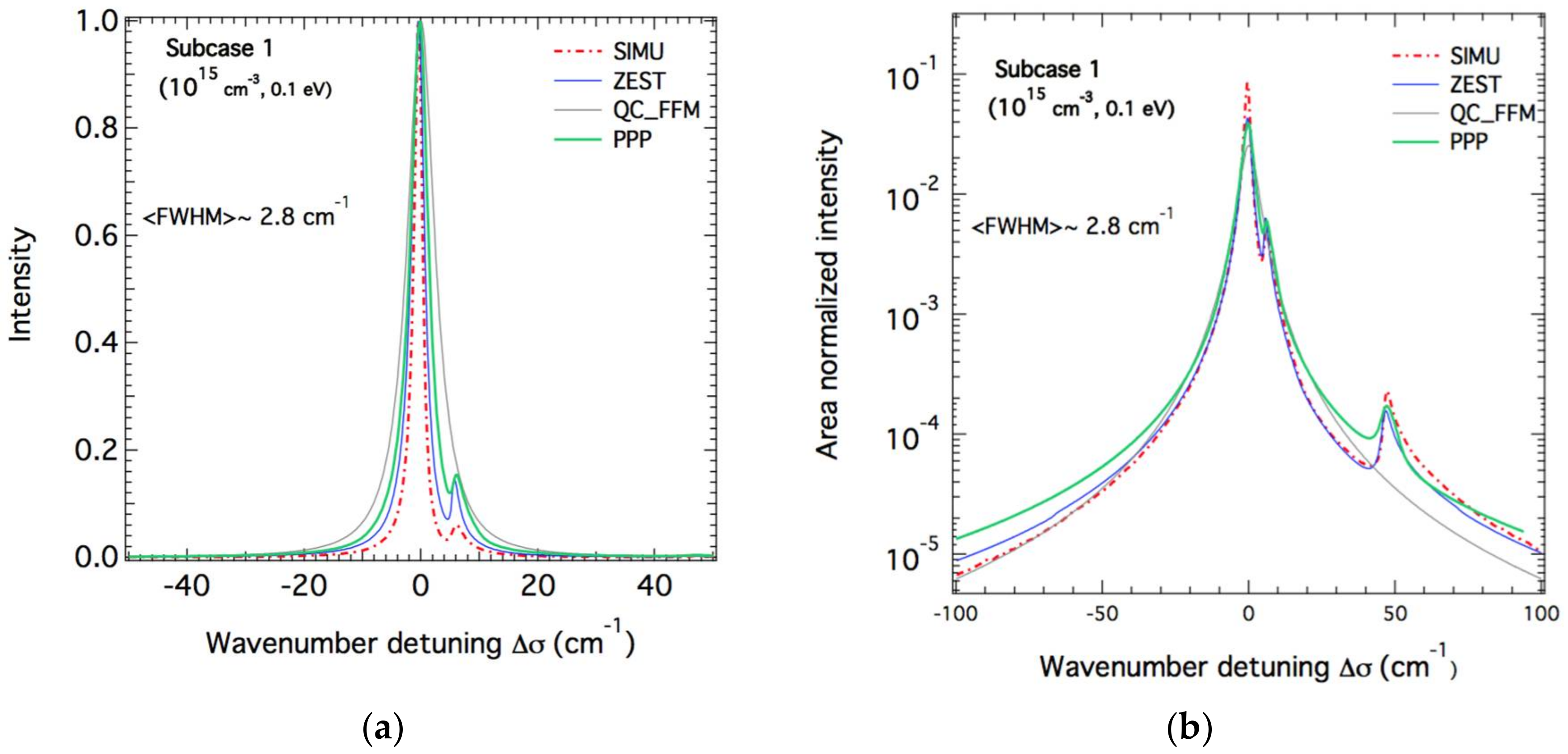
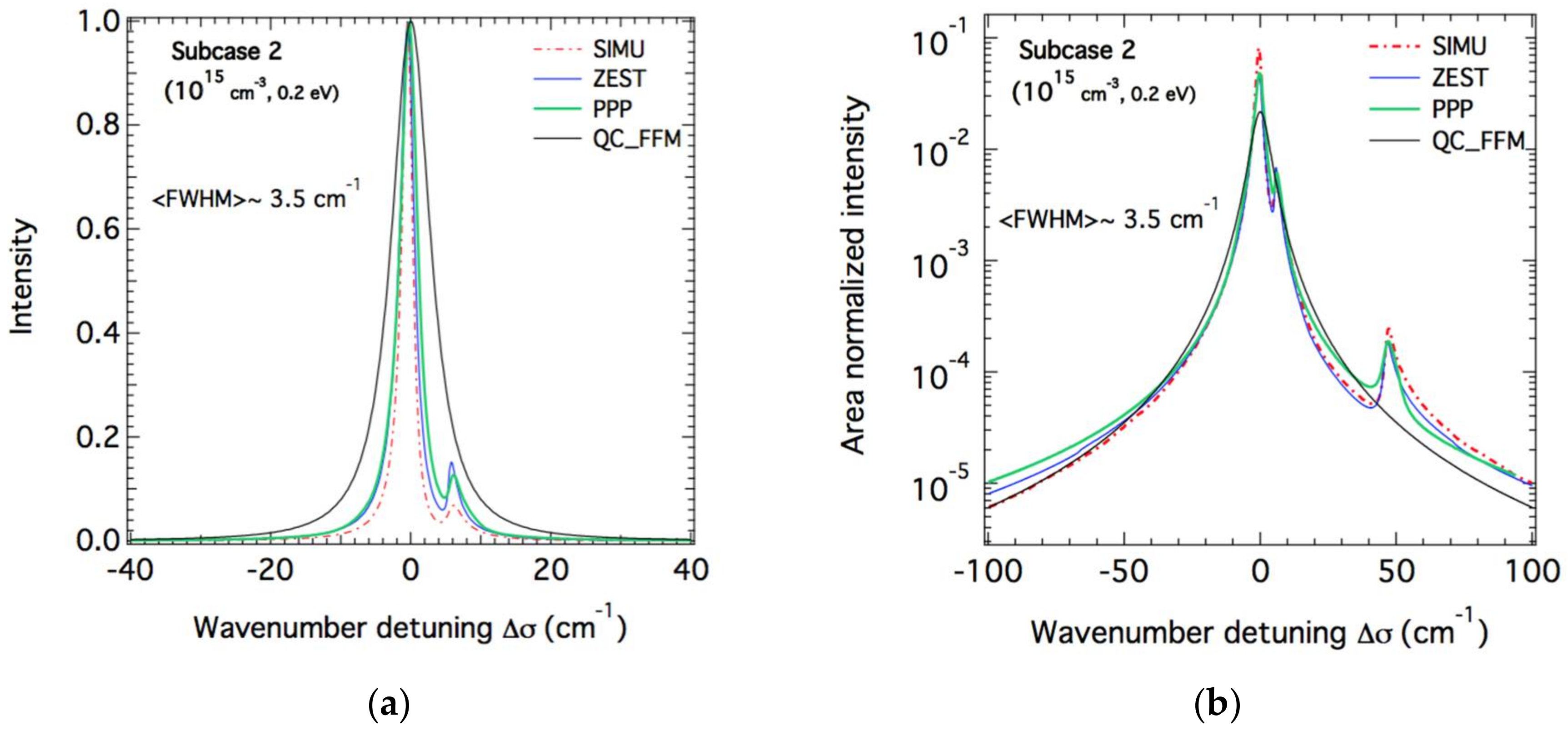
3.1. He i 492 nm Line Profiles for the Lowest Density

The results of the code calculations for the lower density case (n_e = 10¹⁵ cm⁻³) are respectively illustrated for equal ion and electron temperatures of 0.1, 0.2 and 0.4 eV in Figure 1, Figure 2 and Figure 3. For each figure corresponding to a subcase (Subcase 1: 0.1 eV, Subcase 2: 0.2 eV and Subcase 3: 0.4 eV), the profiles were plotted using a logarithmic scale together with the linear scale to point out more clearly the differences. As it can be seen from Figure 1, the calculations carried out by PPP, ZEST, and SimU codes are comparable and agree to some extent. Of course they give different widths with SimU calculations providing the lowest FWHM followed closely by ZEST and PPP. This relative agreement is also seen on the forbidden components. Indeed, the three codes give profiles showing the lateral forbidden components already mentioned previously. The highest lateral peak (closest peak to the line center) represents the 1s2p ¹P°-1s4f ¹F transition while the weakest peak (located far from the line center) refers to the 1s2p ¹P°-1s4p ¹P° transition. An average full width at half maximum (FWHM) of about 2.8 cm⁻¹ has been estimated for this subcase. The profile calculated by QC_FFM is different from all the others. As expected, QC_FFM gave much broader profiles with no forbidden components. Indeed, recall that the QC model is derived assuming (i) a H-like (fully degenerate) atomic system and (ii) a transition with $\Delta n\gg 1$. For these reasons, neither forbidden components nor detailed line core structure (such as a dip in H-β line) can be reproduced. As a result, since the He i n = 4 singlet states at lower densities are far from being degenerate, QC_FFM is very inaccurate and should not be used in real-life scenarios. However, as the plasma density is increased (see below), the atomic system approaches the degenerate-case assumption and the results of QC_FFM become more reliable. Similarly, in the far wings (at detunings exceeding the 1s4d–1s4f separation), the QC model becomes reasonably accurate even for lower densities. This can be seen in the semi-log plots in the figures. When it comes to the second case corresponding to 0.2 eV shown on Figure 2, the situation is identical for SimU, PPP, and ZEST whose calculations are in a relative overall agreement with ZEST calculations being more closer to those of PPP than to those of SimU. All three codes agree in showing forbidden components in terms of positions even though there are differences in their widths and shapes. The weak forbidden component 1s2p ¹P°-1s4p ¹P° is visible on both linear and logarithmic scales while the most central forbidden component 1s2p ¹P°-1s4f ¹F is visible only on the logarithmic scale. The situation is worse for QC_FFM with a large overestimation of the width which is at least two or three times the average one of about 3.5 cm⁻¹ shown on Figure 2. For the last subcase corresponding to a temperature of 0.4 eV shown on Figure 3, again QC_FFM calculations are completely different from all others with a clear overestimation of the broadening. In terms of FWHM, there is no change with respect to the previous subcase with the same average FWHM of 3.5 cm⁻¹. Again one can see the agreement between PPP, ZEST, and SimU which is even better in terms of widths. There are still some small differences in the shapes of the forbidden components.

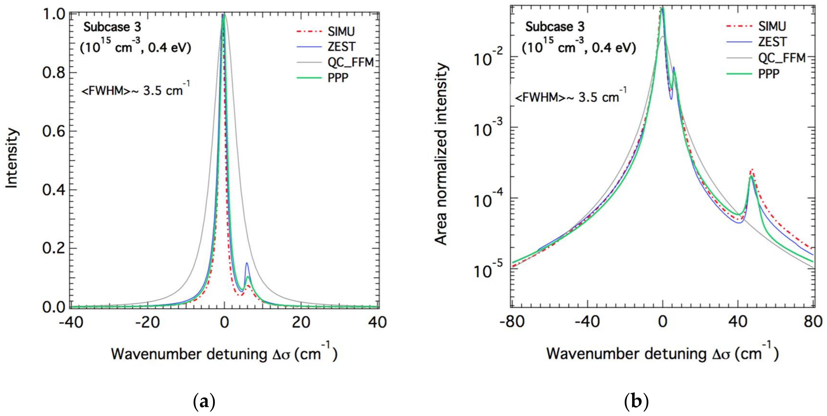
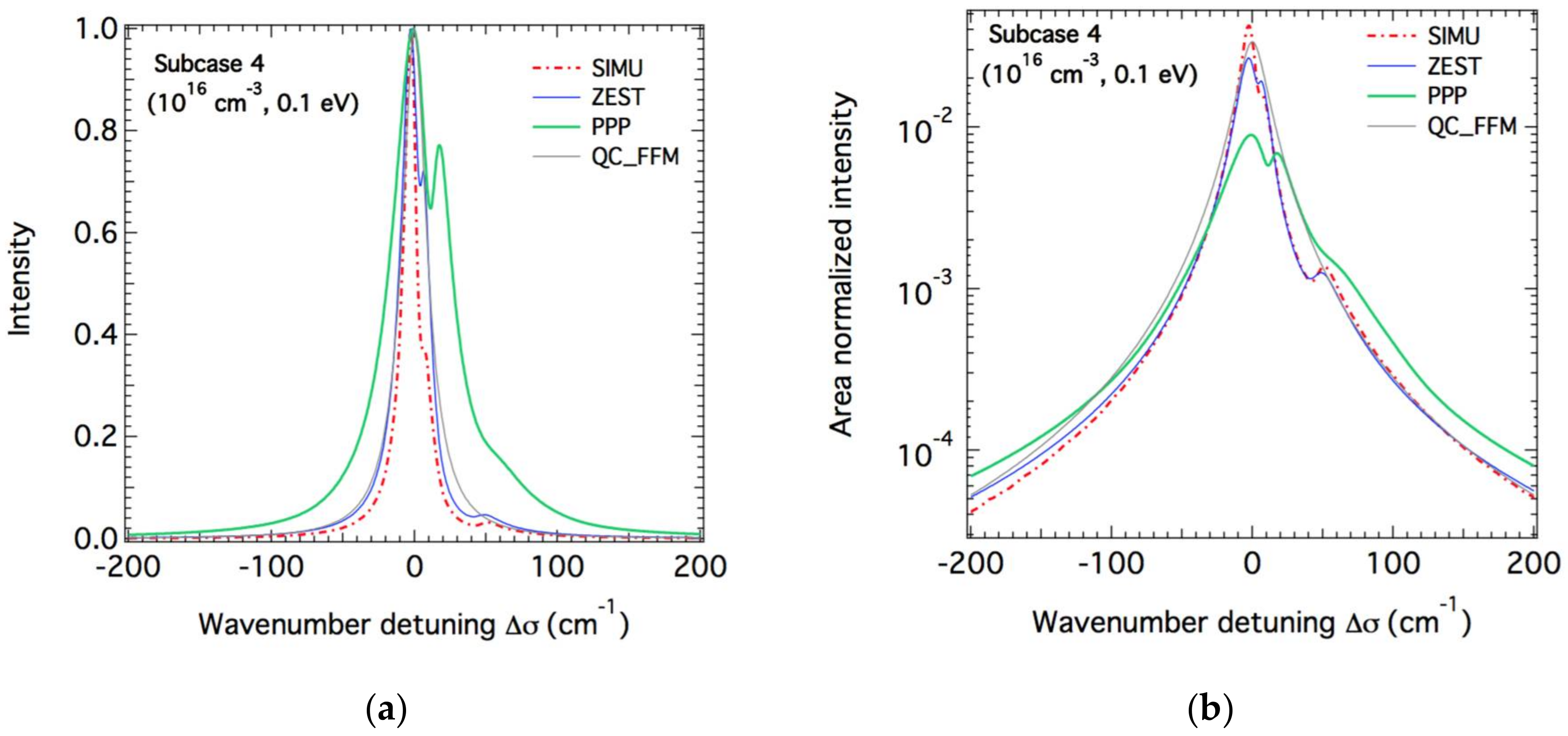
3.2. He i 492 nm Line Profiles for the Highest Density

As for the previous case, the results of code calculations for the higher density case (n_e = 10¹⁶ cm⁻³) with the same temperatures 0.1 (Subcase 4), 0.2 (SUBCASE 5) and 0.4 eV (subcase 6) are respectively shown in Figure 4, Figure 5 and Figure 6. Unlike the previous case, by showing a broadening about twice than the other code calculations, the profiles given by PPP seem to be inadequate for the conditions of this subcase. This is attributed to the frequency independence of the GBK (Griem–Blaha–Kepple) formulation of the [12] collision operator used in this PPP version to treat the line electron broadening electron broadening and to the use of a Holtsmark field distribution for the ions. This demonstrate that the use of a frequency-dependent collision operator may show up narrower profiles as compared to those calculated by a frequency independent operator. For this density, the expected discrepancy between the calculations carried out by the PPP code using the GBK collision operator and those of the other codes are more pronounced confirming the non-validity of this form of collision operators at high densities and low temperatures. One can see that for the remaining calculations, SimU is close to ZEST in terms of widths but differs significantly when it comes to the intensity of the forbidden components. QC_FFM shows higher widths than ZEST and SimU. Similar remarks can be said for the calculations of the second subcase of Figure 4 (0.2 eV). However, the subcase of Figure 6 seems more favorable for all codes. These conditions correspond in terms of results to those of Figure 1, Figure 2 and Figure 3. Except the intensity of the forbidden components, SimU and ZEST, give very close results, especially at the line wings. The widths of the PPP profiles are close to those of QC_FFM.

3.3. Comparison of the FWHM of the He i Line

The FWHM of the He i line vs the electron temperature (0.1, 0.2 and 0.4 eV) deduced from all the synthetic profiles are shown on Figure 7 for two values of the electron density n_e = 10¹⁵ and 10¹⁶ cm⁻³. In part (a) of Figure 7, we can see that the widths deduced from QC_FFM calculations are about twice the average one. The values deduced from the remaining codes agree at higher electron temperatures but show a dispersion with a factor of two at the lowest temperature. In Figure 7b, the value of the FWHM at the lowest electron temperature is much higher than in comparison to other codes. The other widths show some dispersion with a factor 2 to 3 between the codes.

4. Preliminary Comparisons with Experimental Spectra

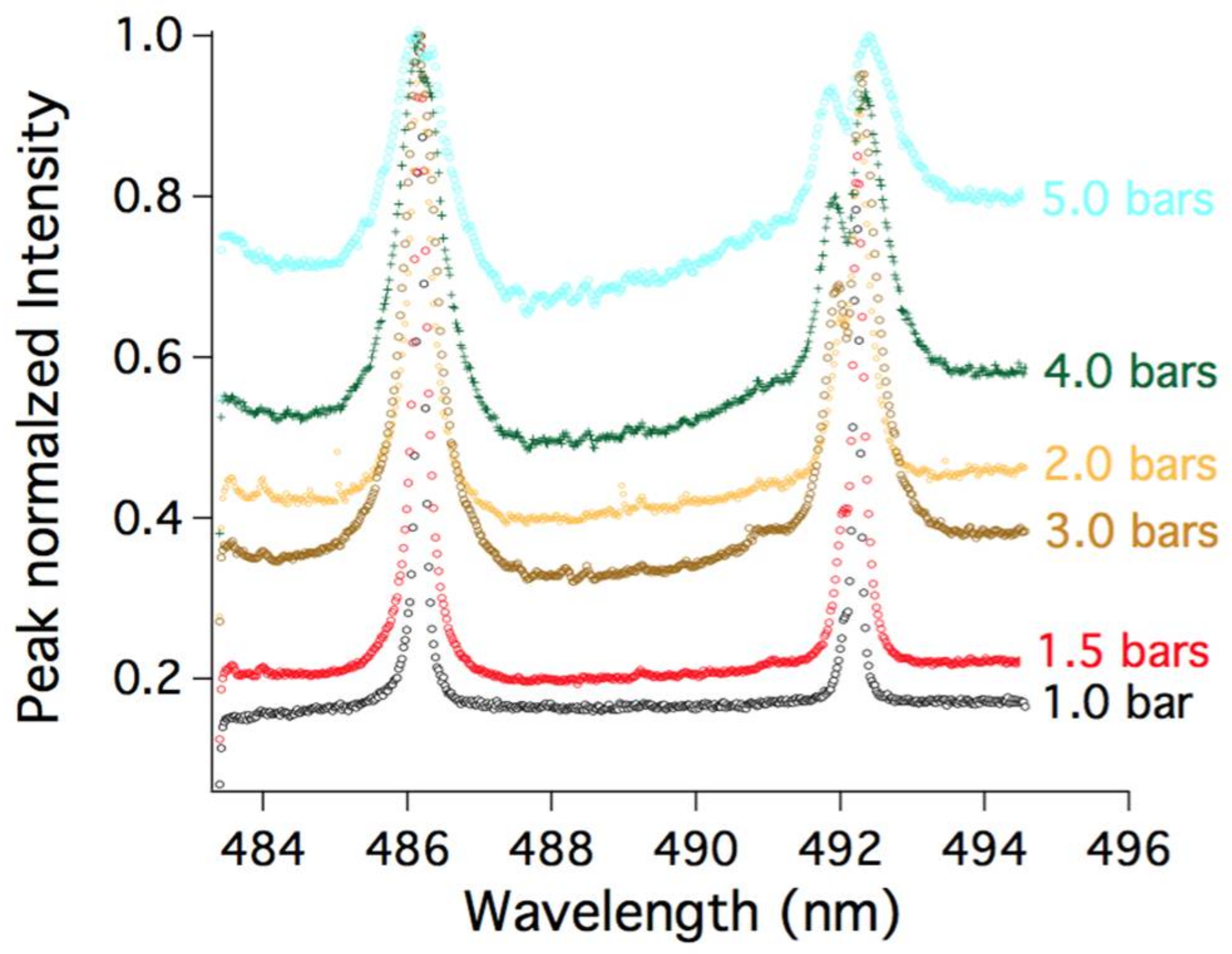
4.1. Experimental Spectra

The experimental spectra proposed for analysis were measured in a corona discharge in helium performed in an electrical engineering laboratory for the study of the dielectric properties of insulators [13,14]. Spectra of the neutral helium 492 nm and its neighboring hydrogen H-β (486.1 nm) lines were measured at room temperature for various values of the pressure. A quartz lens was used to focus the light into a 500-mm-focal-length triple grating spectrograph (Acton Research Corporation; Spectra-Pro-2500i with 1800 groves/mm and 1200/groove/mm gratings). A liquid-N₂-cooled charge coupled device (CCD; Princeton Instruments model 2DCCDTKB-UV/AR) was installed at the exit plane of the spectrograph. The spectral resolution with the 1800 groove/mm grating was 0.09 nm as determined from the spectral profiles of Helium lamp lines. Spectra corresponding to six values of the pressure in the range 1–5 bars are shown in Figure 8. One can see that both helium and hydrogen lines become broader as the pressure is increased indicating an increase in the Stark broadening of both lines. More specifically, it can be also seen that the helium line right peak of each spectrum) presents an increasing asymmetry which is partially due to the forbidden components. Therefore, high pressure spectra with complex features are difficult to reproduce by calculations. That is why only few cases were considered, mainly spectra at pressures of 1 and 1.5 bars. Therefore, the comparisons code-experimental data which are presented here are preliminary and are only used for illustration.

4.2. Broadening of the Neutral Helium Line

The 492 nm line emitted by neutral helium atoms in a corona discharge is broadened by several mechanisms. For the experimental data considered here, the instrumental function was estimated from a helium calibration lamp to be a Gaussian with a FWHM of 0.09 nm [14]. Besides the instrumental function and the natural broadening which are very small, the line may be subject to Stark, Doppler, resonance, and van der Waal broadenings. Resonance and van der Waals broadenings [15], which are due to collisions between neutrals, can be represented by Lorentzian shapes whose FWHM depend on the ratio (P/T) as follows: $\Delta {\lambda }_{res}\propto \left(P/T\right)$ and $\Delta {\lambda }_{vdW}\propto \left(\frac{P}{T^{0.7}}\right)$, where P and T are respectively the pressure and the neutral temperature. For the experimental conditions of the spectra of Figure 8, resonance broadening may be comparable to the other contributing broadenings. However, as this broadening was not retained by all the participating codes, it is ignored here. To evaluate the FWHM of the van der Waals broadening, we have used the expression [16]

$$\Delta {\lambda }_{vdW}=8.18\times {10}^{-26}{\lambda }_0^2\alpha {\overline{R}}^2{}^{2/5}{\left(\frac{T}{\mu }\right)}^{3/10}N,$$

(1)

where is $\mu$ and ${\lambda }_0$ are respectively the reduced mass of the colliding atoms and the central wavelength of the line. ${\overline{R}}^2$ is the average difference of the square radii of the emitter between its upper and lower levels in Bohr radius units while $\alpha$ represents the polarizability of the neutral perturber which is about 2 × 10⁻²⁵ cm⁻³ for helium neutrals. $T$ and $N$ are the gas temperature and density. By introducing the pressure $P$ as a function of $T$ and $N$ for an ideal gas, the van der Waals FWHM (in nm units) reduces to the expression

$$\Delta {\lambda }_{vdW}=2.74\times {10}^{-5}\left(\frac{P}{T^{0.7}}\right),$$

(2)

Values of the van der Waals FWHM calculated with Equation (2) for the conditions of each of the six experimental spectra are shown in

Table 1. Summary of the FWHM of the van der Waals broadening compared with the experimental FWHM of the six experimental spectra of the He i 492 nm line

Pressure (Bars)	$\mathbf{\Delta }{\mathit{\lambda }}_{\mathit{v}\mathit{d}\mathit{W}}$ (nm)	$\mathbf{\Delta }{\mathit{\lambda }}_{\mathit{e}\mathit{x}\mathit{p}}$ (nm)	$\mathbf{\Delta }{\mathit{\lambda }}_{\mathit{v}\mathit{d}\mathit{W}}/\mathbf{\Delta }{\mathit{\lambda }}_{\mathit{e}\mathit{x}\mathit{p}}$ (%)
1	0.045	0.150	30
1.5	0.068	0.228	30
2	0.091	0.283	30
3	0.136	-	-
4	0.182	-	-
5	0.227	-	-

. The van der Waals broadening represents about 30% of the total broadening of the line.

4.3. Preliminary Comparison with an Experimental Spectrum

We present here only a preliminary comparison of some theoretical profiles calculated by three codes PPP, QC_FFM, and ZEST for the case of spectrum 15 b corresponding to a pressure of 1.5 bars. This is illustrated on Figure 9. This figure illustrates the difficulty to fit this spectrum and the difficulty is even higher for the cases of higher pressures. These spectra have been very recently fitted with a genetic algorithm coupled to the PPP code and the fitting results can be found in [17]. However, as the present comparisons of code calculations to the experimental spectra are aimed to highlight any differences between the codes and as resonance broadening was ignored in the fitting of experimental spectra, we cannot draw any reliable conclusion about the inferred plasma densities. One should note that other authors support that the conditions considered in this paper are more relevant to the electric field measurements than to electron density diagnostics [18]. However, this is another issue which deserves to be addressed but it is beyond the scope of this paper.

5. Conclusions

Theoretical pure Stark profiles of the neutral helium 492 nm line calculated by four codes have been compared for plasma conditions supposed to cover those of a corona discharge in helium with traces of hydrogen. These conditions correspond to plasmas of singly ionized helium ions with electron densities of 10¹⁵ and 10¹⁶ cm⁻³ and equal ions and neutral temperatures of 0.1, 0.2 and 0.4 eV. For the lowest density, three codes are in a relative agreement: PPP, SimU, and ZEST showing comparable widths sometimes within a factor up to two with a relatively good agreement concerning the appearance of the forbidden components (lateral components) unlike QC_FFM which overestimates the broadening. For the highest density, the surprise comes from PPP which overestimates in this case the broadening especially at 0.1 eV even if this discrepancy tends to disappear for temperatures higher than 0.4 eV. This discrepancy was expected for two reasons: the use of non-frequency collision operator instead of frequency-dependent one and the use of a Holtsmark field distribution which may not be valid. There is an overall agreement between ZEST, SimU, and QC_FFM (although the later, evidently, is not able to model any forbidden component). For the comparisons with experimental spectra, the task was hard and only few attempts were tried. This is due to the complexity of the spectra showing an asymmetry increasing with increasing pressure in addition to the appearance of the forbidden components whose intensity depends on the pressure too. Only a preliminary comparison has been presented for an illustrative purpose. Since the time these calculations and comparisons have been done, other more recent works have been done and will be published.

References

1. Griem, H.R. Principles of Plasma Spectroscopy; Cambridge University Press: Cambridge, UK, 1997. [Google Scholar]
2. Griem, H.R. Spectral Line Broadening by Plasmas; Academic Press: New York, NY, USA, 1974. [Google Scholar]
3. Stambulchik, E. Review of the 1st spectral line shapes in plasmas code comparison workshop. High Energy Density Phys. 2013, 9, 528. [Google Scholar] [CrossRef]
4. 4th SLSP Workshop. Available online: http://plasma-gate.weizmann.ac.il/projects/slsp/slsp4/ (accessed on 22 February 2018).
5. Sheeba, R.R.; Koubiti, M.; Bonifaci, N.; Gilleron, F.; Mossé, C.; Pain, J.-C.; Stambulchi, E. H-β line in a corona helium plasma: A muli-code line shape comparison. Atoms 2018. in progress. [Google Scholar] [CrossRef]
6. Stambulchik, E.; Maron, Y. A study of ion-dynamics and correlation effects for spectral line broadening in plasma: K-shell lines. J. Quant. Spectrosc. Radiat. Transf. 2006, 99, 730–749. [Google Scholar] [CrossRef]
7. Stambulchik, E.; Alexiou, S.; Griem, H.R.; Kepple, P.C. Stark broadening of high principal quantum number hydrogen Balmer lines in low-density laboratory plasmas. Phys. Rev. E 2007, 75, 016401. [Google Scholar] [CrossRef] [PubMed]
8. Calisti, A.; Khelfaoui, F.; Stamm, R.; Talin, B.; Lee, R.W. Model for the line shapes of complex ions in hot and dense plasmas. Phys. Rev. A 1990, 42, 5433–5440. [Google Scholar] [CrossRef] [PubMed]
9. Stambulchik, E.; Maron, Y. Quasicontiguous frequency-fluctuation model for calculation of hydrogen and hydrogenlike Stark-broadened line shapes in plasmas. Phys. Rev. E 2013, 87, 053108. [Google Scholar] [CrossRef] [PubMed]
10. Gilleron, F.; Pain, J.-C. ZEST: A fast code for simulating Zeeman-Stark line-shape functions. Atoms 2018, 6, 11. [Google Scholar] [CrossRef]
11. Calisti, A.; Mossé, C.; Ferri, S.; Talin, B.; Rosmej, F.; Bureyeeva, L.A.; Lisitsa, V.S. Dynamic Stark broadening as the Dicke narrowing effect. Phys. Rev. E 2010, 81, 016406. [Google Scholar] [CrossRef] [PubMed]
12. Griem, H.R.; Blaha, M.; Kepple, P.C. Stark-profile calculations for Lyman-series lines of one-electron ions in dense plasmas. Phys. Rev. A 1979, 19, 2421. [Google Scholar] [CrossRef]
13. Li, Z.-L.; Bonifaci, N.; Aitken, F.; Denat, A.; von Haeften, K.; Atrazhev, V.M.; Shakhatov, V.A. Spectroscopic investigation of liquid helium excited by a corona discharge: Evidence for bubbles and “red satellites”. Eur. Phys. J. Appl. Phys. 2009, 47, 2821. [Google Scholar] [CrossRef]
14. Rosato, J.; Bonifaci, N.; Li, Z.; Stamm, R. Line shape modeling for the diagnostic of the electron density in a corona discharge. Atoms 2017, 5, 35. [Google Scholar] [CrossRef]
15. Laux, C.O.; Spence, T.G.; Kruger, C.H.; Zare, R.N. Optical diagnostics of atmospheric pressure air plasmas. Plasma Sources Sci. Technol. 2003, 12, 125–138. [Google Scholar] [CrossRef]
16. Yubero, C.; Dimitrijević, M.S.; Garcia, M.C.; Calzada, M.D. Using the van der Waals broadening of the spectral atomic lines to measure the gas temperature of an argon microwave plasma at atmospheric pressure. Spectrochim. Acta B 2007, 62, 169–176. [Google Scholar] [CrossRef]
17. Mossé, C.; Génésio, P.; Bonifaci, N.; Calisti, A. A new procedure to determine the plasma parameters from a genetic algorithm coupled with the spectral line shape PPP. Atoms 2018. submitted. [Google Scholar]
18. Obradović, B.M.; Cvetanović, N.; Ivković, S.S.; Sretenović, G.B.; Kovačević, V.V.; Krstić, I.B.; Kuraica, M.M. Methods for spectroscopic measurement of electric field in atmospheric pressure helium discharges. Eur. Phys. J. Appl. Phys. 2017, 7, 30802. [Google Scholar] [CrossRef]
Figure 1. Theoretical Stark profiles of the He i 492 nm line calculated for helium plasma with an electron density of 1015 cm−3 and a temperature of 0.1 eV for both plasma He+ ions and electrons corresponding to subcase 1. The profiles are centered at 492 nm and expressed as wavenumbers using cm−1 units. (a) Linear scale. (b) The profiles are the same but they are area normalized and plotted using a semi-logarithmic scale to highlight the differences between the different calculations. In both (a,b), the average FWHM is shown. Red dot-dashed line: SimU, solid blue: ZEST, solid green: PPP, solid grey: QC_FFM.
Atoms 06 00019 g001
Figure 2. Same as Figure 1 but for Te = Ti = 0.2 eV.
Atoms 06 00019 g002
Figure 3. Same as Figure 1 and Figure 2 but for Te = Ti = 0.4 eV.
Atoms 06 00019 g003
Figure 4. Theoretical Stark profiles of the He i 492 nm line calculated for a helium plasma with an electron density of 1016 cm−3 and a temperature of 0.1 eV for both plasma He+ ions and electrons. The profiles are centered at 492 nm and expressed as wavenumbers in cm−1 units. Blue: ZEST, green: PPP, grey: QC_FFM, red dot-dashed: SimU. (a) Linear scale. (b) Same profiles but area normalized and plotted using a semi-logarithmic scale.
Atoms 06 00019 g004
Figure 5. Same as Figure 4, but for Te = Ti = 0.2 eV. Same line styles and code colors as Figure 4.
Atoms 06 00019 g005
Figure 6. Same as Figure 4 and Figure 5 with the same line styles and code colors but for Te = Ti = 0.4 eV.
Atoms 06 00019 g006
Figure 7. The He i line full width at half maximum (FWHM) versus the electron temperature as deduced from the profiles calculated by the four codes PPP, QC_FFM, SimU and ZEST. (a) Lowest density (ne = 1015 cm−3). (b) Highest density (ne = 1016 cm−3).
Atoms 06 00019 g007
Figure 8. Superposition of six experimental spectra of the He i 492 nm (right peak) and H-β 486.2 nm (left peak) lines measured at room temperature for pressures in the range 1–5 bars. Black: 1 bar, red: 1.5 bars, light brown: 2 bars, dark brown: 3 bars, green: 4 bars, and blue: 5 bars.
Atoms 06 00019 g008
Figure 9. Preliminary comparisons of the helium 492 nm line profiles calculated by PPP, QC_FFM, and ZEST corresponding to a pressure P = 1.5 bars.
Atoms 06 00019 g009