A New Implementation of the STA Method for the Calculation of Opacities of Local Thermodynamic Equilibrium Plasmas


Racah Institute of Physics, The Hebrew University, 9190401 Jerusalem, Israel
*
Author to whom correspondence should be addressed.
Atoms 2018, 6(3), 35; https://doi.org/10.3390/atoms6030035
Submission received: 10 April 2018
/
Revised: 15 June 2018
/
Accepted: 15 June 2018
/
Published: 21 June 2018
(This article belongs to the Special Issue Atomic and Molecular Opacity Data for Astrophysics)
Abstract
:We present opacity calculations with the newly developed STAR code, which implements the Super-Transition-Array (STA), with various improvements. The model is used to calculate and analyze local thermodynamic equilibrium opacities of mid and high Z elements and of the solar interior plasma. We briefly review the underlying computational model and present calculations for iron and neodymium over a wide range of temperature and density.
1. Introduction
The calculation of atomic opacities from first principles is an important part in the modeling of various astrophysical phenomena, and especially the physics of stellar interior. Opacities quantify the strong coupling between radiation and matter in a hot dense plasma, and therefore, are directly related to the radiative thermal conductivity in stellar interior.
In recent years, a solar composition problem has emerged [1,2], as a result of a revision in the solar photospheric abundances, in which the metallic abundance was significantly decreased [3]. Metallic elements have a significant contribution to the opacity in the solar interior, although they only constitute a few percent of the mixture, since these metallic elements are not completely ionized and give rise to strong bound-bound and bound-free absorption. This gives rise to a connection between the solar composition problem and the theoretical uncertainty in the calculation of opacities at stellar interior conditions [4,5,6,7].
We have recently developed [6,7,8,9,10] the atomic code STAR (STA-Revised), for the calculation of opacities of local thermodynamic equilibrium plasmas, by the STA method [11]. The code was used to investigate and analyze sensitivities and uncertainties in the calculation of solar interior opacities.
In this paper we describe the underlying computational model and present the computational capabilities of STAR. We calculate the opacity spectra of iron, neodymium and the solar mixture, as well as Rosseland and Planck mean free paths for a wide range of temperature and density. We also present maps for the contributions of the different atomic processes to the Rosseland opacity.
2. The Model
The monochromatic opacity is given as a sum of four different processes: (i) photon scattering and (ii) free-free (iii) bound-free and (iv) bound-bound absorption. The cross-section for photon-absorption (including stimulated emission) for the ith component of a mixture plasma at temperature T and density , is written as:
where is Boltzmann’s constant. The monochromatic opacity is by definition the absorption coefficient per unit mass:
where is the atomic mass of the i component and is Avogadro’s constant. The total monochromatic opacity of the mixture is given by the sum of the individual opacities, weighted by the mass fraction:
The Rosseland mean opacity is given by:
with the Rosseland weight function:
where .
A simple way to measure fractional contributions, such as the contribution of different elements in a mixture or different atomic processes, to the total Rosseland mean, is the following: given N individual spectral contributions:
we define the fractional Rosseland contributions by:
where is the Rosseland mean (4) of the cumulative spectra , while for the first contributer .
The photon scattering cross section is written as (see Refs. [10,12] and references therein):
where is the average number of free electrons, is the reduced chemical potential and the Thomson cross-section is
with the fine structure constant and the Bohr radius. , where , corrects the Klein–Nishina cross-section due to the finite temperature and contains corrections for inelastic scattering. The factor contains corrections due to the Pauli blocking as a result of partial degeneracy and includes a relativistic electron dispersion relation. The factor is a correction due to plasma collective effects.
The free-free photoabsorption cross section is calculated via a screened-hydrogenic approximation with a multiplicative degeneracy correction, and is given by:
where the Kramers cross-section is:
with the free electron number density. For the (thermal) averaged free-free Gaunt factor , we use a screened-hydrogenic approximation and a Maxwellian distribution via the tables given in Ref. [13]. Degeneracy is incorporated using the correction factor (see Ref. [10] and references therein).
In principle, the photoexcitation opacity can result from all possible allowed transitions between pairs of bound-states, from all populated electronic configurations in the plasma. In practice, for mid and high-Z elements, typical configurations may contain a huge number of lines [14,15], so that Detailed-Line-Accounting codes [16,17,18,19,20], and the Unresolved-Transition-Array (UTA) method is used to group this huge number of lines [9,21,22,23,24,25]. However, in many situations, for hot-dense plasmas and for , there is an intractable number of populated configurations, and a detailed accounting of all UTAs in the spectra is computationally impossible. In Refs. [10,26] the number of populated relativistic configurations was estimated by the formula:
where:
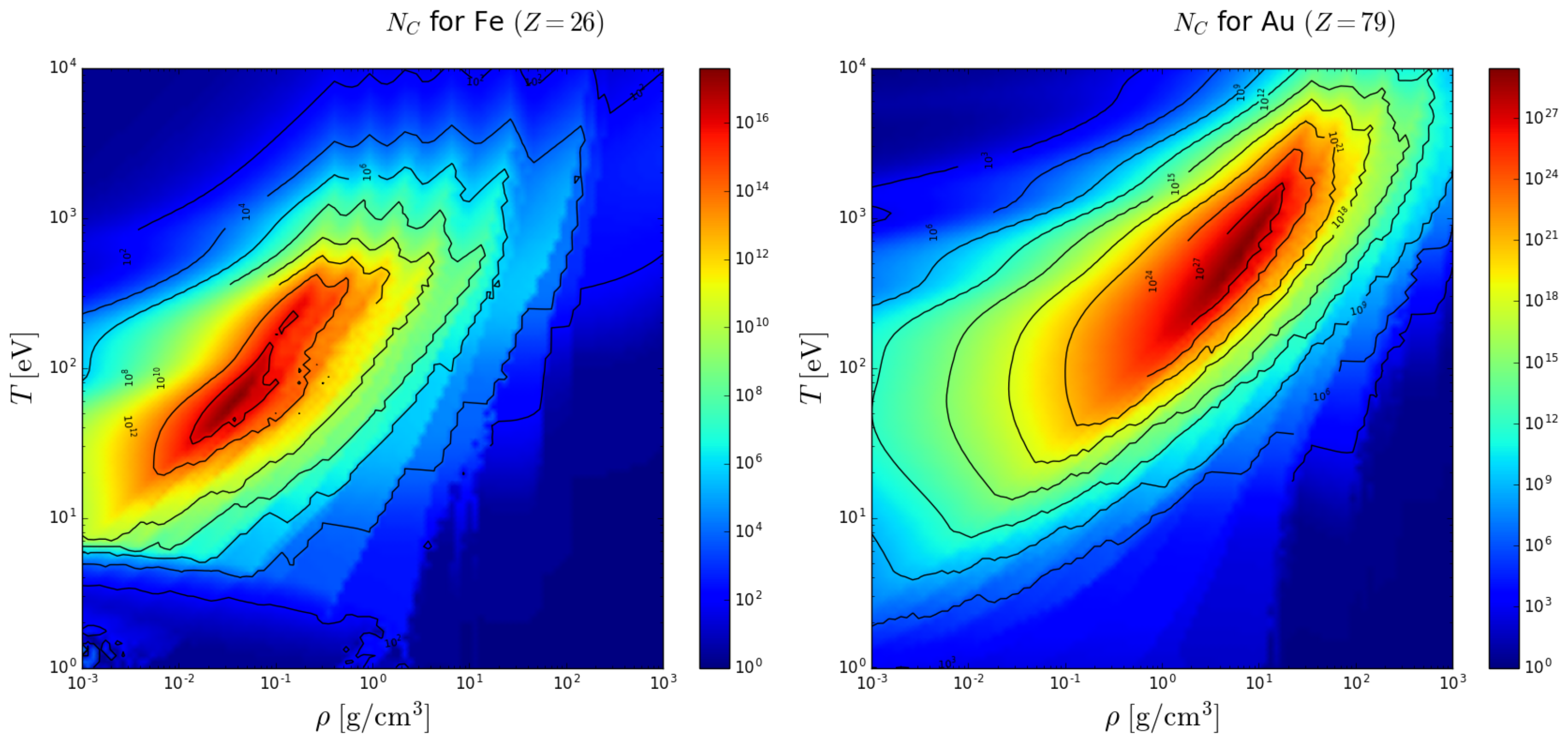
is the variance of the population of shell s, is the Fermi–Dirac distribution, is the orbital degeneracy, is the orbital energy and is the chemical potential. It is seen from Equation (12) that the occupation numbers of shells whose energies are near the Fermi-Dirac step fluctuate, while the other shells are either filled or empty. Thus, when the temperature is high enough, such that there are multiple shells that lie within the Fermi-Dirac step, the number of populated configurations can become huge. A calculation of for iron () and gold () in a wide range of temperature and density is given in Figure 1. The calculations were performed via the ion-sphere model implemented in STAR. It is evident that for iron the number of populated configurations can become larger than ∼, while for gold, this number can become larger than ∼. It is also evident that has a single maximum in temperature for each density, and in density for each temperature. This is explained by the fact that shells become ionized for high temperatures or full for low temperatures, and pressure ionized for high densities. For low densities, shell populations become non-degenerate—which reduces the fluctuations in shells occupation numbers. It is also seen, as expected, that the maximum of for gold has a larger temperature and density than iron has, due to the higher nuclear attraction and number of bound shells.
STAR implements the STA method [11] for the calculation of bound-bound and bound-free photoabsorption spectra. The STA method enables the grouping of the huge number of lines between the enormous number of configurations into large sets, called Super-Transition-Arrays (STAs). The STA moments are calculated analytically via the partition function algebra, and are split into smaller STAs until convergence is achieved. This procedure enables the handling of situations where the number of populated configurations is too large, as shown in Figure 1. STAR also implements several additional advanced capabilities, such as (i) an adaptive integration of resonances in the electronic density of state [27,28,29,30], which has an effect on the bound-free structure and on the self-consistent field average-atom calculation, (ii) ion-sphere and ion-correlation models for the plasma environment [7,27,31,32,33,34] and (iii) stable recursive calculation of partition functions, as in Refs. [8,35,36,37].
3. Opacity Calculations
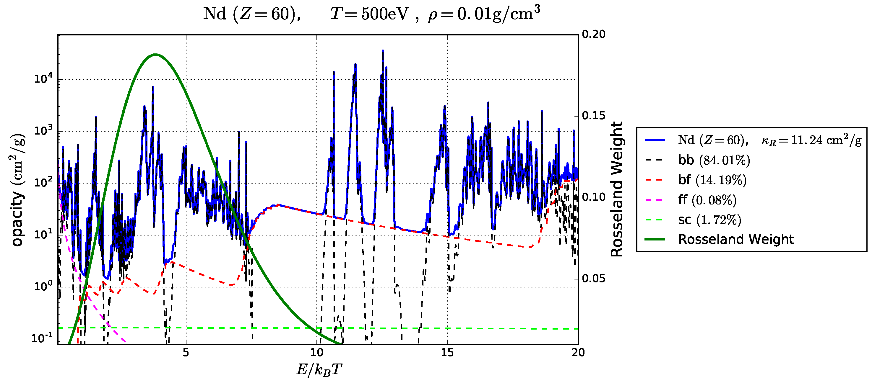
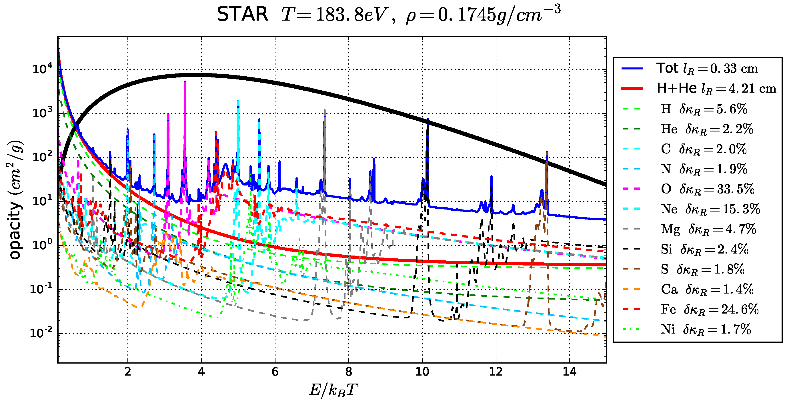
In Figure 2 and Figure 3, spectral opacities for iron () and neodymium () are presented in detail. It is seen in Figure 3 how for neodymium, lines are “condensed” into transition arrays due to the huge number of lines. Figure 4 shows in detail the opacity spectra of the solar mixture at (near the convection zone). It is evident that the opacity contribution of the fully ionized hydrogen and helium, which consist more than of the mixture, is only less than . On the other hand, it is seen that most of the opacity is due to bound-bound and bound-free photoabsorption of various mid-Z elements such as oxygen and neon (via K-shell absorption), as well as iron (via L-shell absorption).
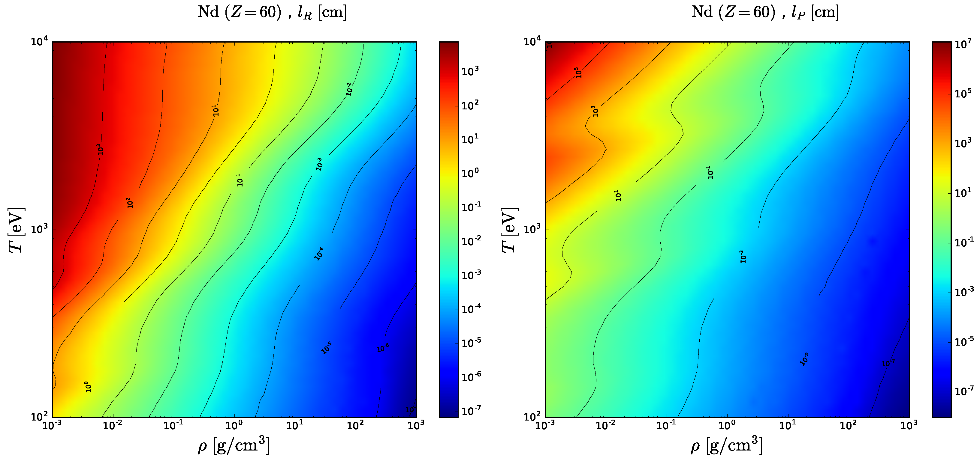
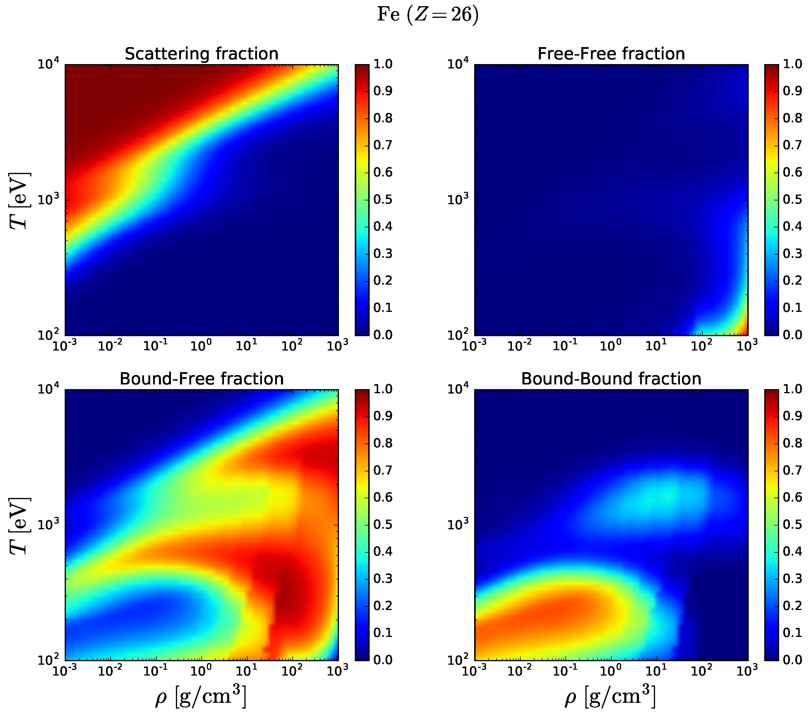
In Figure 5 and Figure 6 we present maps of the Rosseland and Planck mean free paths for iron and neodymium, respectively, over a wide range of temperature (100 –10 ) and density (0.001–1000 ). In Figure 7 and Figure 8 maps for the contributions of the atomic fractions (scattering, free-free, bound-free and bound-bound) to the Rosseland opacity are shown. It is evident that in both cases the bound-bound and bound-free processes are major contributers over most of the temperature-density range, and that the bound-bound contribution is much more dominant for neodymium, due to its higher atomic number.
We note that extensive comparisons between STAR and other widely used opacity codes (specifically, OP [16], OPAL [17] and OPAS [38]), were performed in Ref. [10] for the case solar opacities. These comparisons resulted in a very satisfactory agreement in the Rosseland opacity of the solar mixture of about throughout the solar interior. Spectral opacities and ionic populations of several metallic elements were also compared at the thermodynamic conditions of the solar convection zone, and good agreement was reached.
4. Summary
The new opacity code STAR was presented. The code was used to calculate local thermodynamic equilibrium opacities for iron and neodymium over a wide range of temperature and density. Comparisons of STAR with other widely used atomic codes where performed in a previous publication [10], and a good agreement was reached. We conclude that stellar interior opacities can be calculated and analyzed successfully with the STAR code.
Author Contributions
Equal contribution.
Funding
This research received no external funding.
Conflicts of Interest
The authors declare no conflicts of interest.
References
- Bahcall, J.N.; Basu, S.; Pinsonneault, M.; Serenelli, A.M. Helioseismological implications of recent solar abundance determinations. Astrophys. J. 2005, 618, 1049. [Google Scholar] [CrossRef]
- Bergemann, M.; Serenelli, A. Solar abundance problem. In Determination of Atmospheric Parameters of B-, A-, F- and G-Type Stars; Springer: Cham, Switzerland, 2014; pp. 245–258. [Google Scholar]
- Asplund, M.; Grevesse, N.; Sauval, A.J.; Scott, P. The chemical composition of the sun. arXiv, 2009; arXiv:0909.0948. [Google Scholar] [CrossRef]
- Christensen-Dalsgaard, J.; di Mauro, M.P.; Houdek, G.; Pijpers, F. On the opacity change required to compensate for the revised solar composition. Astron. Astrophys. 2009, 494, 205–208. [Google Scholar] [CrossRef]
- Villante, F.L.; Serenelli, A.M. A quantitative analysis of the solar composition problem. Phys. Procedia 2015, 61, 366–375. [Google Scholar] [CrossRef]
- Krief, M.; Feigel, A.; Gazit, D. Line broadening and the solar opacity problem. Astrophys. J. 2016, 824, 98. [Google Scholar] [CrossRef]
- Krief, M.; Kurzweil, Y.; Feigel, A.; Gazit, D. The effect of ionic correlations on radiative properties in the solar interior and terrestrial experiments. Astrophys. J. 2018, 856, 135. [Google Scholar] [CrossRef]
- Krief, M.; Feigel, A. The effect of first order superconfiguration energies on the opacity of hot dense matter. High Energy Density Phys. 2015, 15, 59–66. [Google Scholar] [CrossRef]
- Krief, M.; Feigel, A. Variance and shift of transition arrays for electric and magnetic multipole transitions. High Energy Density Phys. 2015, 17 (Pt B), 254–262. [Google Scholar] [CrossRef]
- Krief, M.; Feigel, A.; Gazit, D. Solar opacity calculations using the super-transition-array method. Astrophys. J. 2016, 821, 45. [Google Scholar] [CrossRef]
- Bar-Shalom, A.; Oreg, J.; Goldstein, W.H.; Shvarts, D.; Zigler, A. Super-transition-arrays: A model for the spectral analysis of hot, dense plasma. Phys. Rev. A 1989, 40, 3183. [Google Scholar] [CrossRef]
- Huebner, W.F.; Barfield, W.D. Opacity; Springer: Cham, Switzerland, 2014. [Google Scholar]
- Van Hoof, P.A.M.; Williams, R.J.R.; Volk, K.; Chatzikos, M.; Ferland, G.J.; Lykins, M.; Porter, R.L.; Wang, Y. Accurate determination of the free–free gaunt factor–i. non-relativistic gaunt factors. Mon. Not. R. Astron. Soc. 2014, 444, 420–428. [Google Scholar] [CrossRef]
- Gilleron, F.; Pain, J.-C. Efficient methods for calculating the number of states, levels and lines in atomic configurations. High Energy Density Phys. 2009, 5, 320–327. [Google Scholar] [CrossRef]
- Scott, H.A.; Hansen, S.B. Advances in NLTE modeling for integrated simulations. High Energy Density Phys. 2010, 6, 39–47. [Google Scholar] [CrossRef] [Green Version]
- Seaton, M.J.; Yan, Y.; Mihalas, D.; Pradhan, A.K. Opacities for stellar envelopes. Mon. Not. R. Astron. Soc. 1994, 266, 805–828. [Google Scholar] [CrossRef] [Green Version]
- Iglesias, C.A.; Rogers, F.J. Updated OPAL opacities. Astrophys. J. 1996, 464, 943. [Google Scholar] [CrossRef]
- Bar-Shalom, A.; Klapisch, M.; Oreg, J. HULLAC, an integrated computer package for atomic processes in plasmas. J. Quant. Spectrosc. Radiat. Transf. 2001, 71, 169–188. [Google Scholar] [CrossRef]
- Gu, M.F. The flexible atomic code. Can. J. Phys. 2008, 86, 675–689. [Google Scholar] [CrossRef]
- Fontes, C.J.; Zhang, H.L.; Abdallah, J., Jr.; Clark, R.E.H.; Kilcrease, D.P.; Colgan, J.; Cunningham, R.T.; Hakel, P.; Magee, N.H.; Sherrill, M.E. The Los Alamos suite of relativistic atomic physics codes. J. Phys. B: Atom. Mol. Opt. Phys. 2015, 48, 144014. [Google Scholar] [CrossRef]
- Moszkowski, S.A. On the energy distribution of terms and line arrays in atomic spectra. Prog. Theor. Phys. 1962, 28, 1–23. [Google Scholar] [CrossRef]
- Bauche-Arnoult, C.; Bauche, J.; Klapisch, M. Variance of the distributions of energy levels and of the transition arrays in atomic spectra. Phys. Rev. A 1979, 20, 2424. [Google Scholar] [CrossRef]
- Bauche-Arnoult, C.; Bauche, J.; Klapisch, M. Variance of the distributions of energy levels and of the transition arrays in atomic spectra. II. configurations with more than two open subshells. Phys. Rev. A 1982, 25, 2641. [Google Scholar] [CrossRef]
- Bauche-Arnoult, C.; Bauche, J.; Klapisch, M. Variance of the distributions of energy levels and of the transition arrays in atomic spectra. III. case of spin-orbit-split arrays. Phys. Rev. A 1985, 31, 2248. [Google Scholar] [CrossRef]
- Bauche-Arnoult, C.; Bauche, J. Statistical approach to the spectra of plasmas. Phys. Scr. 1992, 1992, 58. [Google Scholar] [CrossRef]
- Nikiforov, A.F.; Novikov, V.G.; Uvarov, V.B. Quantum-Statistical Models of Hot Dense Matter: Methods for Computation Opacity and Equation of State; Springer Science & Business Media: Basel, Switzerland, 2006; Volume 37. [Google Scholar]
- Liberman, D.A. Self-consistent field model for condensed matter. Phys. Rev. B 1979, 20, 4981. [Google Scholar] [CrossRef]
- Wilson, B.; Sonnad, V.; Sterne, P.; Isaacs, W. Purgatorio a new implementation of the Inferno algorithm. J. Quant. Spectrosc. Radiat. Transf. 2006, 99, 658–679. [Google Scholar] [CrossRef]
- Pénicaud, M. An average atom code for warm matter: application to aluminum and uranium. J. Phys. Condens. Matter 2009, 21, 095409. [Google Scholar] [CrossRef] [PubMed]
- Ovechkin, A.A.; Loboda, P.A.; Novikov, V.G.; Grushin, A.S.; Solomyannaya, A.D. RESEOS—A model of thermodynamic and optical properties of hot and warm dense matter. High Energy Density Phys. 2014, 13, 20–33. [Google Scholar] [CrossRef]
- Rozsnyai, B.F. Relativistic Hartree-Fock-Slater calculations for arbitrary temperature and matter density. Phys. Rev. A 1972, 5, 1137–1149. [Google Scholar] [CrossRef]
- Rozsnyai, B.F. Photoabsorption in hot plasmas based on the ion-sphere and ion-correlation models. Phys. Rev. A 1991, 43, 3035. [Google Scholar] [CrossRef] [PubMed]
- Starrett, C.E.; Saumon, D.; Daligault, J.; Hamel, S. Integral equation model for warm and hot dense mixtures. Phys. Rev. E 2014, 90, 033110. [Google Scholar] [CrossRef] [PubMed]
- Blenski, T.; Piron, R. Free-energy functional of the debye–hückel model of two-component plasmas. High Energy Density Phys. 2017, 24, 28–32. [Google Scholar] [CrossRef]
- Wilson, B.G.; Liberman, D.A.; Springer, P.T. A deficiency of local density functionals for the calculation of self-consistent field atomic data in plasmas. J. Quant. Spectrosc. Radiat. Transf. 1995, 54, 857–878. [Google Scholar] [CrossRef]
- Wilson, B.G.; Gilleron, F.; Pain, J.-C. Further stable methods for the calculation of partition functions in the superconfiguration approach. Phys. Rev. E 2007, 76, 032103. [Google Scholar] [CrossRef] [PubMed]
- Gilleron, F.; Pain, J.-C. Stable method for the calculation of partition functions in the superconfiguration approach. Phys. Rev. E 2004, 69, 056117. [Google Scholar] [CrossRef] [PubMed]
- Blancard, C.; Cossé, P.; Faussurier, G. Solar Mixture Opacity Calculations Using Detailed Configuration and Level Accounting Treatments. Astrophys. J. 2012, 745, 10. [Google Scholar] [CrossRef]
Figure 1.
Maps on the temperature-density plane of the number of occupied relativistic configurations (see Equation (12)) for iron (upper pane) and gold (lower pane).
Figure 1.
Maps on the temperature-density plane of the number of occupied relativistic configurations (see Equation (12)) for iron (upper pane) and gold (lower pane).

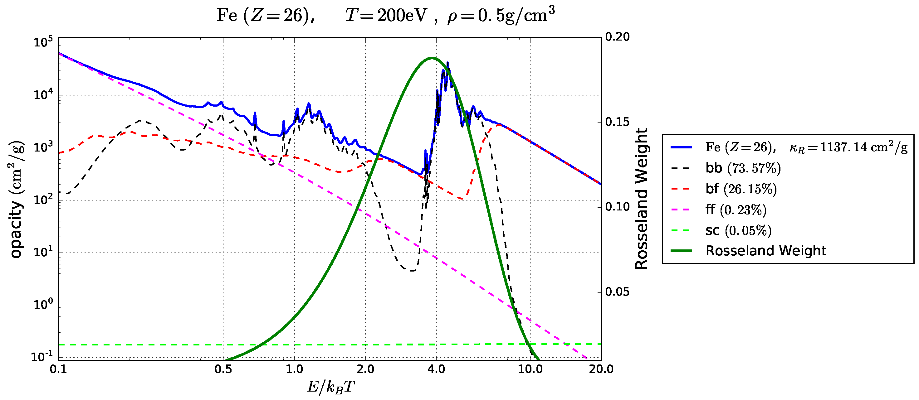
Figure 2.
Opacity spectrum, calculated by STAR, for iron () at T = 200 and = 0.5 . The total (blue), as well as the bound-bound (black), bound-free (red), free-free (magenta) and scattering (lime) opacity spectra are shown (left axis), together with the Rosseland wieght function (green, right axis). The Rosseland mean opacity and the processes contributions to it, are given in the legend.

Figure 3.
Same as Figure 2, for neodymium () at T = 500 and = 0.01 .
Figure 3.
Same as Figure 2, for neodymium () at T = 500 and = 0.01 .

Figure 4.
The opacity spectrum for the solar mixture at the conditions found at (near the solar convection-zone) where T = 183.8 and = 0.1745 . The total opacity due to all element in the solar mixture (solid blue) is compared to the opacity due to hydrogen and helium only (solid red), and the spectra of various individual elements, with a Rosseland opacity contribution that is larger than (dashed lines). The Rosseland mean free path and the Rosseland opacity contributions , are listed in the legend. The Rosseland weight function (solid black) is also shown.

Figure 5.
Maps on the temperature-density plane of the Rosseland (left pane) and Planck (right pane) photon absorption mean free paths.
Figure 5.
Maps on the temperature-density plane of the Rosseland (left pane) and Planck (right pane) photon absorption mean free paths.

Figure 6.
Same as Figure 5, for neodymium.
Figure 6.
Same as Figure 5, for neodymium.

Figure 7.
Maps on the temperature-density plane of the scattering (upper left pane), free-free (upper right pane), bound-free (lower left pane) and bound-bound (lower right pane) atomic processes contributions to the Rosseland opacity for iron.
Figure 7.
Maps on the temperature-density plane of the scattering (upper left pane), free-free (upper right pane), bound-free (lower left pane) and bound-bound (lower right pane) atomic processes contributions to the Rosseland opacity for iron.

Figure 8.
Same as Figure 7, for neodymium.
Figure 8.
Same as Figure 7, for neodymium.

© 2018 by the authors. Licensee MDPI, Basel, Switzerland. This article is an open access article distributed under the terms and conditions of the Creative Commons Attribution (CC BY) license (http://creativecommons.org/licenses/by/4.0/).
Share and Cite
MDPI and ACS Style
Krief, M.; Feigel, A.; Gazit, D. A New Implementation of the STA Method for the Calculation of Opacities of Local Thermodynamic Equilibrium Plasmas. Atoms 2018, 6, 35. https://doi.org/10.3390/atoms6030035
AMA Style
Krief M, Feigel A, Gazit D. A New Implementation of the STA Method for the Calculation of Opacities of Local Thermodynamic Equilibrium Plasmas. Atoms. 2018; 6(3):35. https://doi.org/10.3390/atoms6030035
Chicago/Turabian StyleKrief, Menahem, Alexander Feigel, and Doron Gazit. 2018. "A New Implementation of the STA Method for the Calculation of Opacities of Local Thermodynamic Equilibrium Plasmas" Atoms 6, no. 3: 35. https://doi.org/10.3390/atoms6030035
Note that from the first issue of 2016, this journal uses article numbers instead of page numbers. See further details here.