Review of Recent Advances in the Analytical Theory of Stark Broadening of Hydrogenic Spectral Lines in Plasmas: Applications to Laboratory Discharges and Astrophysical Objects

Physics Department, 206 Allison Lab, Auburn University, Auburn, AL 36849, USA
Atoms 2018, 6(3), 50; https://doi.org/10.3390/atoms6030050
Submission received: 26 June 2018
/
Revised: 22 July 2018
/
Accepted: 1 August 2018
/
Published: 3 September 2018
(This article belongs to the Special Issue Stark Broadening of Spectral Lines in Plasmas)
Abstract
:There is presented an overview of the latest advances in the analytical theory of Stark broadening of hydrogenic spectral lines in various types of laboratory and astrophysical plasmas. They include: (1) advanced analytical treatment of the Stark broadening of hydrogenic spectral lines by plasma electrons; (2) center-of-mass effects for hydrogen atoms in a nonuniform electric field: applications to magnetic fusion, radiofrequency discharges, and flare stars; (3) penetrating-ions-caused shift of hydrogenic spectral lines in plasmas; (4) improvement of the method for measuring the electron density based on the asymmetry of hydrogenic spectral lines in dense plasmas; (5) Lorentz–Doppler broadening of hydrogen/deuterium spectral lines: analytical solution for any angle of observation and any magnetic field strength, and its applications to magnetic fusion and solar physics; (6) Revision of the Inglis-Teller diagnostic method; (7) Stark broadening of hydrogen/deuterium spectral lines by a relativistic electron beam: analytical results and applications to magnetic fusion; (8) Influence of magnetic-field-caused modifications of the trajectories of plasma electrons on shifts and relative intensities of Zeeman components of hydrogen/deuterium spectral lines: applications to magnetic fusion and white dwarfs; (9) Influence of magnetic-field-caused modifications of trajectories of plasma electrons on the width of hydrogen/deuterium spectral lines: applications to white dwarfs; (10) Stark broadening of hydrogen lines in plasmas of electron densities up to or more than Ne~1020 cm−3; and, (11) The shape of spectral lines of two-electron Rydberg atoms/ions: a peculiar Stark broadening.
Table of Contents
- Introduction
- Advanced Analytical Treatment of the Stark Broadening of Hydrogenic Spectral Lines by Plasma Electrons
- Center-of-Mass Effects for Hydrogen Atoms in a Nonuniform Electric Field: Applications to Magnetic Fusion, Radiofrequency Discharges, and Flare Stars.
- New Source of Shift of Hydrogenic Spectral Lines in Plasmas: Analytical Treatment of the Effect of Penetrating Ions
- Revision of the Method for Measuring the Electron Density Based on the Asymmetry of Hydrogenic Spectral Lines in Dense Plasmas
- Lorentz–Doppler Broadening of Hydrogen/Deuterium Spectral Lines: Analytical Solution for Any Angle of Observation and any Magnetic Field Strength, and Its Applications to Magnetic Fusion and Solar Physics
- Revision of the Inglis-Teller Diagnostic Method
- Stark Broadening of Hydrogen/Deuterium Spectral Lines by a Relativistic Electron Beam: Analytical Results and Applications to Magnetic Fusion
- Influence of Magnetic-Field-Caused Modifications of Trajectories of Plasma Electrons on Shifts and Relative Intensities of Zeeman Components of Hydrogen/Deuterium Spectral Lines: Applications to Magnetic Fusion and White Dwarfs
- Influence of Magnetic-Field-Caused Modifications of trajectoRies of Plasma Electrons on the Width of Hydrogen/Deuterium Spectral Lines: Applications to White Dwarfs
- Stark Broadening of Hydrogen Lines in Plasmas of Electron Densities up to or More Than Ne~1020 cm−3
- The Shape of Spectral Lines of Two-Electron Rydberg Atoms/Ions: A Peculiar Stark Broadening
- Conclusions
1. Introduction
Stark broadening of hydrogenic spectral lines remains as an important tool for spectroscopic diagnostics of various types of laboratory and astrophysical plasmas. This is because laboratory and astrophysical plasmas contain various types of electric fields, such as the ion microfield, the electron microfield, fields of different kinds of the electrostatic plasma turbulence, and laser/maser fields penetrating into plasmas. All of these kinds of electric fields, differing by their statistical properties, strength, frequency, and possible polarization, cause a garden variety of the types of Stark broadening of spectral lines in plasmas.
Therefore, this research area is very important both fundamentally and practically, the latter being due to numerous applications of plasmas. The practical applications range from the controlled thermonuclear fusion to plasma-based lasers and plasma sources of incoherent X-ray radiation, as well as technological microwave discharges.
Studies that are related to this research area over its lifetime are too numerous to be listed here in their entirety. So, we refer here to seven books [1,2,3,4,5,6,7], published over the last 25 years, and to the references therein.
Our review focuses at latest advances in the analytical theory of the Stark broadening of hydrogenic spectral lines in plasmas. Studying the Stark broadening of hydrogenic lines is important from the theoretical point of view for two reasons: (1) it is a deeply fundamental problem of the simplest, two-particle bound Coulomb system immersed in a multi-particle Coulomb system of free charges (plasma) exhibiting long-range interactions—as was noted by Lisitsa [8]; (2) hydrogenic atoms/ions possess a higher algebraic symmetry than its geometrical symmetry, thus allowing for significant analytical advances in the Stark broadening problem, and therefore yielding a deep physical insight.
The Stark broadening of hydrogenic spectral lines in plasmas has also a great practical importance. This is because hydrogenic spectral lines are employed for diagnosing plasmas in magnetic fusion and laser fusion machines, as well as in powerful Z-pinches (used for producing X-ray and neutron radiation, ultra-high pulsed magnetic fields), in X-ray lasers, in low-temperature technological discharges for plasma processing, and in astrophysics (especially in solar physics and in physics of flare stars and white dwarfs).
As for focusing at the advances in the analytical theory (versus simulations), the following should be noted. Of course, simulations are important as the third powerful research methodology—in addition to theories and experiments: large-scale codes have been created to simulate lots of complicated phenomena. However, first, not all large-scale codes are properly verified and validated, as illustrated by some well-known failures of large-scale codes (see, e.g., [9,10]). Second, fully-numerical simulations are generally not well-suited for capturing the so-called emergent principles and phenomena, such as, e.g., conservation laws and preservation of symmetries, as explained in [9]. Third, as any fully-numerical method, they lack the physical insight.
2. Advanced Analytical Treatment of the Stark Broadening of Hydrogenic Spectral Lines by Plasma Electrons
The theory of the Stark broadening of hydrogenlike spectral lines by plasma electrons, developed by Griem and Shen [11] and are later presented also in books [12,13], is usually referred to as the Conventional Theory, hereafter CT, also known as the standard theory. (Further advances in the theory of the Stark broadening of hydrogenlike spectral lines by plasma electrons can be found, e.g., in books [5,7] and references therein.) In the CT, the perturbing electrons are considered moving along hyperbolic trajectories in the Coulomb field of the effective charge Z − 1 (in atomic units), where Z is the nuclear charge of the radiating ion. In other words, in the CT, there was made a simplifying assumption that the motion of the perturbing electron can be described in frames of a two-body problem, one particle being the perturbing electron and the other “particle” being the charge Z − 1.
However, in reality, one have to deal with a three-body problem: the perturbing electron, the nucleus, and the bound electron. Therefore, trajectories of the perturbing electrons should be more complicated.
In paper [14], the authors took this into account by using the standard analytical method of separating rapid and slow subsystems—see, e.g., book [15]. The characteristic frequency of the motion of the bound electron around the nucleus is much higher than the characteristic frequency of the motion of the perturbing electron around the radiating ion. Therefore, the former represents the rapid subsystem and the latter represents the slow subsystem. This approximate analytical method allows for a sufficiently accurate treatment in situations where the perturbation theory fails—see, e.g., book [15].
By applying this method, the authors obtained in [14] more accurate analytical results for the electron broadening operator than in the CT. They showed by examples of the electron broadening of the Lyman lines of He II that the allowance for this effect increases with the electron density Ne, becomes significant already at Ne~1017 cm−3 and very significant at higher densities. Here, are some details.
The first step in the method of separating rapid and slow subsystems is to “freeze” the slow subsystem (perturbing electron) and to find the analytical solution for the energy of the rapid subsystem (the radiating ion) that would depend on the frozen coordinates of the slow subsystem (in the case studied in [14] it was the dependence on the distance R of the perturbing electron from the radiating ion). To the first non-vanishing order of the R-dependence, the corresponding energy in the parabolic quantization was given by
where and = n1 − n2 are the principal and electric quantum numbers, respectively, of the Stark state of the radiating ion; n1 and n2 are the parabolic quantum numbers of that state.
The next step in this method is to consider the motion of the slow subsystem (perturbing electron) in the “effective potential” Veff(R), consisting of the actual potential plus Enq(R). Since the constant term in Equation (2.1) does not affect the motion, the effective potential for the motion of the perturbing electron could be represented in the form
For the spectral lines of the Lyman series, since the lower (ground) state b of the radiating ion remains unperturbed (up to/including the order ~1/R2), the coefficient β is
For other hydrogenic spectral lines, for taking into account both the upper and the lower states of the radiating ion, the coefficient β can be expressed as
The motion in the potential from Equation (2.2) allows an exact analytical solution. In particular, the relation between the scattering angle and the impact parameter becomes (see, e.g., book [16])
Here, and are the energy and the angular momentum of the perturbing electron, respectively. Since the angular momentum can be written in terms of the impact parameter as
then a slight rearrangement of Equation (2.5) yielded
In the CT, after calculating the S matrices for weak collisions, the electron broadening operator becomes (in atomic units)
where is the scattering angle for the collision between the perturbing electron and the radiating ion and the operator is
Here, f(v) is the velocity distribution of the perturbing electrons, is the reduced mass of the system “perturbing electron—radiating ion”; r is the radius-vector operator of the bound electron (which scales with Z as 1/Z).
So, after solving Equation (2.7) for and substituting the outcome in Equation (2.8), a more accurate expression for the electron broadening operator can be obtained. In [14], to get the message across in the simplest form, the authors solved Equation (2.7) by expanding it in powers of β.
After combining the contributions from weak and strong collisions, the authors obtained the following final results for the electron broadening operator:
for the non-Lyman lines and
for the Lyman lines. Here, and below log[…], stands for the natural logarithm.
For determining the significance of the effect of non-hyperbolic trajectories manifested by the third term in braces in Equation (2.10) or Equation (2.11), the authors evaluated the ratio of that term to the first two terms in the same braces
for the non-Lyman lines or the ratio
for the Lyman lines.
Table 1 presents the values of the ratio from Equation (2.13) for several Lyman lines of He II at the temperature T = 8 eV and the electron density cm−3 [14].
Figure 1 shows the ratio from Equation (2.13) versus the electron density Ne for the Stark components of the electric quantum number |q| = 1 of Lyman-alpha (n = 2), Lyman-beta (n = 3), and Lyman-gamma (n = 4) lines of He II at the temperature T = 8 eV.
It is seen that, for the electron broadening of the Lyman lines of He II, the allowance for the effect considered in [14] is indeed becomes significant already at electron densities Ne~1017 cm−3 and it increases with the growth of the electron density. The authors noted that when the ratio, formally calculated by Equation (2.13), becomes comparable to unity, this is the indication that the approximate analytical treatment based on expanding Equation (2.7) up to the first order of parameter β, is no longer valid. In this case, the calculations should be based on solving Equation (2.7) with respect to ρ without such approximation.
3. Center-of-Mass Effects for Hydrogen Atoms in a Nonuniform Electric Field: Applications to Magnetic Fusion, Radiofrequency Discharges, and Flare Stars
In the recent paper [17], there was studied whether or not the Center-of-Mass (CM) motion and the relative motion can be separated for hydrogen atoms in a nonuniform electric field. For hydrogenic atoms/ions in a uniform electric field, it was well-known that the CM and relative motions can be separated rigorously (exactly)—see, e.g., [18]. As for hydrogenic atoms/ions in a nonuniform electric field, there seemed to be nothing about the separation (or non-separation) of the CM and relative motions in the literature, to the best knowledge of the author of [17].
So, the author of [17] first treated a general case by considering a system of two charges e1 and e2 of masses m1 and m2, respectively, in a nonuniform electric field that is represented by the potential φ. After substituting
so that R and r are the coordinates that are related to the CM motion and the relative motion, and proceeding from the Lagrangian L to the Hamiltonian H, there was obtained the following expression for the latter [17]:
R = (m1r1 + m2r2)/(m1 + m2),
r = r2 − r1,
H = HCM(R, P) + U(R, r) + Hr(r, p)
Here,
is the Hamiltonian of the CM, P being the momentum of the CM motion;
is the Hamiltonian of the relative motion, p being the momentum of the relative motion;
is the coupling of the CM and relative motions. In Equation (3.6)
is the reduced mass of the two particles, and
is a nonuniform electric field (in the expansion of the electric potential, the terms higher than the dipole one were disregarded). In Equation (3.6) and below, for any two vectors A and B, the notation AB stands for the scalar product (also known as the dot-product) of the two vectors.
HCM(R, P) = P2/[2(m1 + m2)] + (e1 + e2)φ(R)
Hr(r, p) = p2/(2μ) + e1e2/r
U(R, r) = μ(e1/m1 − e2/m2)rF(R)
μ = m1m2/(m1 + m2)
F(R) = −dφ(R)/dR
Thus, Equations (3.3) and (3.6) showed that at the presence of a nonuniform electric field, the CM motion and the relative motion are coupled (by U(R, r) from Equation (3.6)), and therefore, rigorously speaking, they cannot be separated. However, in the case where m1 << m2, the CM and relative motions can be separated by using the approximate analytical method of separating rapid and slow subsystems: in this case, the characteristic frequency of the relative motion is much greater than the characteristic frequency of the CM motion, so that the former and the latter are the rapid and slow subsystems, respectively. By applying this method (details of this method that can be found, e.g., in [15]) the author of [17] achieved the pseudoseparation of the CM motion and the relative motion and obtained the following expression for the effective Hamiltonian of the CM motion:
HCM,eff(R, P) = P2/[2(m1 + m2)]+(e1 + e2)φ(R) − (3n|q|ħ2/2)[1/(m1e2) + 1/(m2|e1|)] F(R)cos[θ(R)]
Here, θ(R) is the polar angle of the vector F(R), the z-axis being chosen along the unperturbed Runge-Lenz vector A; q is the electric quantum number (q = n1 − n2, where n1 and n2 are the parabolic quantum numbers).
The author of [17] emphasized that he treated the CM coordinate R as the dynamical variable (which generally depends on time) and that the Hamiltonian HCM,eff(R, P) from Equation (3.9) can be used to solve for the CM motion. This was the primary distinction of his work from papers where the CM coordinate of a hydrogenic atom/ion in a nonuniform electric fields was considered to be fixed.
In the particular case of hydrogen atoms, one has
where e > 0 is the electron charge, me and mp are the electron and proton masses, respectively. Then, Equation (3.9) simplifies to [17]:
e1 = e, e2 = −e, μ = memp/(me + mp)
HCM,eff(R, P) = P2/(2m) − [3n|q|ħ2/(2μe)] F(R)cos[θ(R)], m = (me + mp)
Next, the author of [17] considered the situation where the nonuniform electric field is due to the nearest (to the hydrogen atom) ion of the positive charge Ze and mass mi in a plasma that is located at the distance R from the hydrogen atom. Then, the Hamiltonian from Equation (3.11) was rewritten as
HCM,eff(R, P) = P2/(2m) − (D/R2)cosθ, D = [3n|q|ħ2/(2μ)] Z, cosθ = AR/AR
This Hamiltonian represents a particle of mass m in the dipole potential. Since this particle is relatively heavy (m >> me), its motion can be described classically and the corresponding classical solution is well-known—see, e.g., paper [19]. For this physical system, the radial motion can be exactly separated from the angular motion resulting in the following radial equation:
where ECM is the total energy of the particle. This equation allows for the following exact general solution:
m[R(dR/dt) + (dR/dt)2] = ECM
R(t) = (2ECMt2/m + 2R0v0t + R02)1/2, R0 = R(0), v0 = (dR/dt)t=0
It was well-known that in plasmas of relatively low electron densities Ne, the Stark broadening of the most intense hydrogen lines, i.e., the lines corresponding to the radiative transitions between the levels of the low principal quantum numbers (such as, e.g., Ly-alpha, Ly-beta, H-alpha, etc.), is dominated by the ion dynamical broadening—see, e.g., publications [5,20,21,22,23,24,25]. The corresponding validity condition is presented in Appendix of paper [17]. In the so-called “conventional theory” of the dynamical Stark broadening (also known as the “standard theory”) [26,27,28,29], the relative motion within the pair “radiator—perturber” was assumed to occur along a straight line—as for a free motion (in our case the radiator is a hydrogen atom and the perturber is the perturbing ion).
However, from the preceding discussion in paper [17] it followed that in the more advanced approach, the relative motion within the pair “radiator-perturber” should be treated as the motion in the dipole potential—(D/R2)cosθ, as seen from Equation (3.12). This approach modifies the cross-sections σ(V0) of so-called optical collisions, i.e., the cross-sections of collisions leading to virtual transitions inside level a between its sublevels and to virtual transitions inside level b between its sublevels, resulting in the broadening of Stark components of the hydrogen spectral line. The ion dynamical broadening operator Φab is related to σ(V0), as follows
where V0 is the relative velocity within the pair “radiator-perturber” at t = 0.
Φab(t) = −∫ dV0 f(V0) Ni V0 σ(V0)
By considering the motion within the pair “radiator-perturber” in the reference frame where the perturbing ion is at rest, the authors of [17] obtained the following analytical expression for the matrix elements of the operator σ
where Q0
and
and
and
where
and C is the so-called strong collision constant (C ≤ 2). In the utmost right part of Equation (3.20), the temperature T is in eV and the electron density Ne is in cm−3.
αβ(σ)βα,A,D = 2π·αβ(K2)βαQ0{ln[(exp(2b2) − 1)1/2(1/w4 − 1)1/4/21/2] − b2/2 + [1/(4w2)]ln[(1 + w2)/(1 − w2)]}
Q0 = 2Z2ħ2/(3μ2V02)
αβ(K2)βα = (9/8)[n2(n2 + q2 − m2 − 1) − 4nqn`q` + n`2(n`2+q`2 − m`2 − 1)]
b = [2C/(3Z)]1/2(n2 + n`2)1/2/(n2 − n`2)
w = [2eħ/(μT)][(n2 + n`2)ZmrNe]1/2 = 8.99 × 10⁻¹⁰[(n2 + n`2)ZNemr/mp ]1/2/T
mr = (me + mp)mi/(me + mp+ mi)
For presenting the effect of the CM motion in the universal form, it is convenient (as the authors of [17] did) to introduce the ratio of the cross-section αβ(σ)βα,A,D to the corresponding cross-section αβ(σ)βα,G from the conventional theory by Griem [29]. The ratio of the cross-sections is essentially the same as the ratio of widths γαβ,A,D/γαβ,G:
ratio = αβ(σ)βα,A,D/αβ(σ)βα,G = γαβ,A,D/γαβ,G = {ln[(exp(2b2) − 1)1/2(1/w4 − 1)1/4/21/2] − b2/2 + [1/(4w2)]ln[(1 + w2)/(1 − w2)]}/{ln[b/(wC1/2)] + 0.356}
This ratio is a universal function of just two dimensionless parameters w and b that are applicable for any set of the five parameters Ne, T, n, n`, and C.
The authors of [17] provided numerical examples for some laboratory and astrophysical plasmas where the allowance for the CM motion significantly affects the ion dynamical Stark width. The first example was edge plasmas of magnetic fusion machines (such as, e.g., tokamaks), characterized by the electron density Ne = (1014–1015) cm−3 and the temperature of one or few eV (see, e.g., review [30]). For these plasma parameters, the Stark broadening of the most intense hydrogen spectral lines (Ly-alpha, Ly-beta, H-alpha, etc.) can be dominated by the ion dynamical broadening (see, e.g., [5,20,21,22,23,24,25]).
The second example was plasmas in the atmospheres of flare stars. They are characterized by practically the same range of plasma parameters as the edge plasmas of magnetic fusion machines—see, e.g., book [31] and paper [32].
Figure 2 presents this ratio (for the Hα line emitted from a hydrogen plasma) versus the electron density Ne at T = 1 eV for C = 2 (solid line) and for C = 3/2 (dashed line). It is seen that the allowance for the CM motion increases the ion dynamical Stark width of the Hα line in these kinds of plasmas by up to (15–20)%.
Another example from [17] relates to the plasmas of radiofrequency discharges, such as, e.g., those studied in papers [33,34,35]. The plasma parameters, e.g., in the experiments [33,34], are Ne = 1.2 × 1013 cm−3 and T = (1850–2000) K, i.e., T = (0.16–0.17) eV. Figure 3 presents this ratio (for the Hα line emitted from a hydrogen plasma) versus the electron density Ne at T = 0.17 eV for C = 2 (solid line) and for C = 3/2 (dashed line). It is seen that the allowance for the CM motion increases the ion dynamical Stark width of the Hα line in these kinds of plasmas by up to (15–20)%.
Thus, in addition to the fundamental importance, the results paper [17] seem to also have practical importance for spectroscopic diagnostics of laboratory and astrophysical plasmas.
4. New Source of Shift of Hydrogenic Spectral Lines in Plasmas: Analytical Treatment of the Effect of Penetrating Ions
4.1. Preamble
Red shifts of spectral lines (hereafter, SL) play an important role in astrophysics. Indeed, the relativistic (cosmological and gravitational) red shifts (see, e.g., book by Nussbaumer and Bieri [36]) are at the core of models of the Universe and of tests for the general relativity. However, for inferring the relativistic red shifts from the observed red shifts it is required to allow for the Stark shift of SL. Hydrogen and hydrogenlike (hereafter, H-like) SL in plasmas are usually shifted to the red by electric microfields—see, e.g., books by Griem [2] and by Oks [5] and references therein. Besides, in laboratory plasmas, measurements of the Stark shift can supplement measurements of the Stark width and thus enhance the plasma diagnostics—specifically the determination of the electron density (see, e.g., paper by Parigger et al. [37]).
In papers [38,39], there was described a new source of the Stark shift of hydrogenic SL—in addition to the previously known sources of the shift (we call the latter “standard shifts”). The new source of shift is due to configurations where the perturbing ion is within the bound electron cloud (“penetrating configurations”). The contribution to the shift from penetrating configurations is a product of two factors. The first fact is the statistical weight of penetrating configurations, which is relatively small. The second factor—the shift relevant to penetrating configurations—is relatively large. In papers [38,39] it was shown that the product of these two factors could exceed (sometimes, very significantly) the total standard shift.
In paper [38] the focus was at highly-excited (high-n) hydrogen SL, such as, e.g., Balmer lines of n = 13–17, studied in astrophysical and laboratory observations at the electron density Ne~1013 cm−3 by Bengtson and Chester [34]. Specifically, the authors of [34] presented the red shifts of these SL observed in the spectra from Sirius and in the spectra from a radiofrequency discharge plasma in the laboratory: both types of the observations yielded red shifts that exceeded the corresponding “standard” theoretical shifts by orders of magnitude. In paper [38], it was shown that for the high-n hydrogen lines, the contribution to the red shift from penetrating configurations is by orders of magnitude greater than the standard theoretical and that the allowance for this additional red shift removes the existed huge discrepancy between the observed and theoretical shifts of those high-n hydrogen SL.
In paper [39], the focus was on the contribution to the shift from penetrating configurations for hydrogenlike (H-like) SL. As an example, the authors of [39] compared their theoretical results with the experimental shift of the Balmer-alpha SL of He II 1640 A measured in a laboratory plasma by Pittman and Fleurier [40]. It was shown in [39] that the allowance for this new additional red shift leads to a good agreement with the measured shift from [40] for the entire range of the electron density being employed in that experiment, while without this new shift the standard shifts underestimated the measured shift by factors between two and five.
4.2. “Standard” Shifts of Hydrogenic Spectral Lines
One of the most significant “standard” contributions to the shift of H-like SL is caused by quenching, non-zero Δn (Griem paper [41]), and elastic, zero Δn (Boercker and Iglesias paper [42]) collisions with plasma electrons—hereafter, the electronic shift (see also Griem paper [43]).
For H-like lines, one should also take into account a so-called plasma polarization shift (PPS). It plays an important role in explaining the observed shifts of the high-n H-like SL—see, e.g., books by Griem [2] and by Salzman [9] and paper by Renner et al. [44]. The PPS is less significant for the low-n H-like SL. Physically, the PPS is caused by the redistribution of plasma electrons due to the attraction to the radiating ion. When only plasma electrons inside the orbit of the bound electron were taken into account, the resulting theoretical PPS was blue (such as, e.g., in paper by Berg et al. [45]). Later, it was found that after the allowance for redistributed plasma electrons both outside and inside the bound electron orbit, the resulting theoretical PPS becomes red. However, theoretical results for red PPS by different authors differ by a factor of two—more details and the references will be provided below, while comparing the theoretical and experimental results.
Then, there is a controversial issue of the “standard’ shift caused by plasma ions-hereafter, the standard ionic shift. Various existing calculations were based on the multipole expansion with respect to the ratio rrms/R (in the binary description of the ion microfield) or with respect to the analogous parameter rrmsF1/2 (in the multi-particle description of the ion microfield F). Here, rrms is the root-mean-square value of the radius-vector of the atomic electron (rrms~n2/Z1, where Z1 is the nuclear charge), and R is the separation between the nucleus of the radiating atom/ion and the nearest perturbing ion. We use the atomic units here and below.
The dipole term of the expansion (~1/R2 or ~F) does not lead to any shift of a hydrogenic SL. Indeed, each pair of the Stark components, as characterized by the electric quantum numbers q and −q, is symmetric with respect to the unperturbed frequency ω0 of the hydrogenic line—symmetric concerning both the displacement from ω0 and the intensity. Here, q = n1 − n2, where n1and n2 are the first two of the three parabolic quantum numbers (n1n2 m). The next, quadrupole term of the expansion (~1/R3 or ~F3/2) does not shift the center of gravity of hydrogenic lines. This was rigorously proven in paper [46]. Namely, after allowing for the quadrupole corrections to both the energies/frequencies and the intensities, and then summing up over all the Stark components of a hydrogenic SL, the center of gravity shift becomes exactly zero at any fixed value of R or F.
Thus, within the approach based on the multipole expansion, the first non-vanishing ionic contribution to the shift of hydrogenic SL is supposed to originate from the next term of the multipole expansion: from the term ~1/R2 or ~F2. In processing this term, many authors considered only the quadratic Stark (QS) effect—see papers by Griem [43] and by Könies and Günter [47,48]:
Here, Z2 is the charge of perturbing ions; the superscript (4) at ΔEQS specifies that this term is of the fourth order with respect to the small parameter rrms/R.
However, first, the corrections of this order to the energies are of the same order as the corrections to the intensities, as noted in paper by Demura et al. [49]. Therefore, calculations in Könies and Günter papers [47,48] were inconsistent because they took into account the quadratic Stark corrections only to energies.
Second, there is an even more important flaw in papers by Griem [43] and by Könies and Günter [47,48], as follows. The above Equation (4.1) was obtained by using the dipole term of the multipole expansion treated in the second order of the perturbation theory. However, the quadrupole term, processed in the second order of the perturbation theory, and the octupole term, processed in the 1st order of the perturbation theory, in fact also yield energy corrections ~1/R4—this was shown as early as in 1969 by Sholin [50]. The rigorous energy correction of the order ~1/R4 can be obtained in the form (given in Sholin paper [50] and presented also in book by Komarov et al. [51]):
Apparently, it is inconsistent to allow for one term and to neglect two other terms of the same order of magnitude.
Nevertheless, from table III of Griem paper [43] it is clear that the ionic shift ΔE(4) due to the quadratic Stark effect is by one or more orders of magnitude smaller than the corresponding electronic shift (and that while the latter is red, the former is blue). A more consistent calculation of the ionic shift ΔE(4) does not change the fact that it is just a very small correction to the corresponding electronic shift and is even a smaller correction to the sum of the corresponding electronic shift and the PPS.
An intermediate summary: the standard shift can be represented with the accuracy, sufficient for comparison with experiments/observations, by the electronic shift for hydrogen SL, or by the sum of the electronic shift and the PPS for H-like SL, while the standard ionic shift can be neglected.
Table 2 presents the electronic shift Se of the hydrogen SL H13–H17, calculated by formulas from papers by Griem [41,43], and their comparison with the shifts from paper by Bengtson & Chester [34] observed in astrophysical and laboratory plasmas, the latter being a radofrequency discharge of Ne~1013 cm−3. It is seen that the electronic shift is by orders of magnitude smaller than both the shift of the SL H14, H15, H17 observed in the spectrum of Sirius and the shift of the SL H13, H15, and H17 observed in the laboratory plasma.
4.3. New Source of the Red Shift and the Comparison with Experiments/Observations
The standard approaches to calculating the ionic contribution to the shift of hydrogenic SL, discussed in the previous section, used the multipole expansion in terms of the parameter rrms/R that was considered to be small. All the terms of the multipole expansion, starting from the quadrupole term, at the averaging over the distribution of the separation R between the nucleus of the radiating atom/ion and the nearest perturbing ion, led to integrals diverging at small R. These diverging integrals were evaluated one way or another, e.g., by introducing cutoffs. However, the mere fact that the integrals were diverging was an indication that the standard approach did not provide a consistent complete description of the ionic contribution to the shift.
The fact is that the standard approaches disregarded configurations where rrms/R > 1, i.e., where the nearest perturbing ion is within the radiating atom/ion (below we call them “penetrating configurations”). The contribution to the ionic shift from penetrating configurations is a product of two factors. The first fact is the statistical weight of penetrating configurations, which is relatively small. The second factor—the shift relevant to penetrating configurations—is relatively large. In papers [38,39] it was shown that the product of these two factors could exceed the total standard shift.
For penetrating configurations, it is appropriate to use the expansion in terms of the parameter R/rrms < 1 in the basis of the spherical wave functions of the so-called “united atom”, which is a hydrogenic ion of the nuclear charge Z1 + Z2. The energy expansion has the form (see, e.g., book by Komarov et al. [51], Equations (5.10)–(5.12)):
E = −(Z1 + Z2)2/(2n2) + O(R2/rrms2)
Therefore, the first non-vanishing contribution to the shift of the energy level is
S(n) = −(Z1 + Z2)2/(2n2) − [−Z12/(2n2)] = −(2Z1Z2 + Z22)/(2n2)
While S(n) scales ~1/n2, the statistical weight I(n) increases with growing n more rapidly than ~n2, as shown in [38,39]. Therefore, the sign of the shift of the spectral line is determined by the sign of the shift of the upper level: it is negative in the frequency scale, so that it is positive in the wavelength scale—the red shift.
The final step is the integration over the distribution of the interionic distances, which can be obtained from the distribution of the ion microfield that is presented in papers by Held [52] and Held et al. [53], where these authors took into account ion-ion correlations and the screening by plasma electrons. The upper limit of the integration could be taken as the root mean square size of the bound electron cloud.
The results of calculating this contribution to the shift of the hydrogen SL H13–H17 by for the parameters corresponding to the observations from by Bengtson and Chester [34] (Ne = 1.2 × 1013 cm−3, Z1 = Z2 = 1), are shown in Table 3 in the column Si,penetr—according to paper [39]. The sum Si,penetr + Se is shown in the column Stot. The theoretical error margin is shown only for the latter and it is primarily due to the approximate way of estimating Si,penetr.
The following can be seen from Table 3.
- For the SL H13, there is an excellent agreement between the total theoretical shift Stot and the experimental shift Sexp. No data for the shift of this SL from Sirius.
- For the SL H14, there is a good agreement of the total theoretical shift with the shift of this SL observed from Sirius and a satisfactory agreement (within the error margins) with the experimental shift of this SL.
- For the SL H15, there is a good agreement of the total theoretical shift with the shift of this SL observed from Sirius and a satisfactory agreement (almost within the error margins) with the experimental shift of this SL.
- For the SL H16, there is a satisfactory agreement (within the error margins) of the total theoretical shift with both the shift of this SL as observed from Sirius and the experimental shift of this SL.
- For the SL H17, there is a satisfactory agreement (within the error margins) of the total theoretical shift with the shift of this SL observed from Sirius, but a disagreement with the experimental shift of this SL; however, the latter disagreement is not anymore by two orders of magnitude, as it was the case before the allowance for the shift by penetrating ions, but rather just by a factor of two (after allowing for the error margins).
As another example taken from paper [39], here is the comparison of various theoretical sources of the shift (including the shift by penetrating ions) for the He II Balmer- line with the experimental shift of this line that was obtained by Pittman and Fleurier [40] for the electron densities in the range of Ne = (0.3 − 2.3) × 1017 cm−3. In Figure 4, the experimental shifts Δλexp are shown by circles. The theoretical shift by Griem [41,43] ΔλGriem, with which Pittman and Fleurier [40] compared their experimental results, is shown by the dashed blue line.
It is seen that there was a huge discrepancy between the experimental red shift Δλexp and the theoretical red shift by Griem. The discrepancy is by a factor of 2.6 at Ne = 1017 cm−3 and is increasing to almost a factor of five at Ne = 2.2 × 1017 cm−3.
In Figure 4, the PPS ΔλPPS is shown by the dotted red line. The sum ΔλGrie + ΔλPPS is shown by the dash-dotted brown line. It is seen that even after adding the PPS to Griem’s shift, their sum still underestimates the experimental shift at least by a factor of two.
The shift due to penetrating ions ΔλPI is shown by the solid green line. The sum ΔλGriem+ ΔλPPS + ΔλPI is presented in Figure 4 by the dashed purple band (the width of the band reflects the theoretical error of this sum, originated from the relative inaccuracy of the relatively simple model from [39] and from the theoretical uncertainty of the PPS). It is seen that adding the shift due to the penetrating ions brings the total shift into a good agreement with the experimental shift.
5. Revision of the Method for Measuring the Electron Density Based on the Asymmetry of Hydrogenic Spectral Lines in Dense Plasmas
In paper [54], there was previously proposed and experimentally implemented a new diagnostic method for measuring the electron density Ne while using the asymmetry of hydrogenic spectral lines in dense plasmas. In that paper, in particular, from the experimental asymmetry of the C VI Lyman-delta line that was emitted by a vacuum spark discharge, the electron density was deduced to be Ne = 3 × 1020 cm−3. This value of Ne was in good agreement with the electron density that was determined from the experimental widths of C VI Lyman-beta and Lyman-delta lines.
Later, this diagnostic method was employed also in the experiment presented in paper [55]. In that laser-induced breakdown spectroscopy experiment, the electron density Ne~3 × 1017 cm−3 was determined from the experimental asymmetry of the H I Balmer-beta (H-beta) line.
When compared to the traditional method of deducing Ne from the experimental widths of spectral lines, the new method has the following advantages. First, the traditional method requires measuring widths of at least two spectral lines (to isolate the Stark broadening from competing broadening mechanisms), while for the new diagnostic method it is sufficient to obtain the experimental profile of just one spectral line. Second, the traditional method would be difficult to implement if the center of the spectral lines is optically thick, while the new diagnostic method can still be used even in this case.
In the theory underlying this new diagnostic method, the contribution of plasma ions to the spectral line asymmetry was calculated only for configurations where the perturbing ions are outside the bound electron cloud of the radiating atom/ion (non-penetrating configurations). In paper [56], the authors took into account the contribution to the spectral line asymmetry from penetrating configurations, where the perturbing ion is inside the bound electron cloud of the radiating atom/ion. While calculating the corresponding corrections to the wave functions and to the intensity of spectral line components, they employed the robust perturbation theory developed in paper [57].
The theory from paper [57], which is applicable to degenerate quantum systems, constructs the perturbation approach to the operator of an additional conserved quantity (rather than to the Hamiltonian operator). This theory avoids infinite summations that are encountered in the standard perturbation theory. For the problem considered in paper [56], the additional conserved quantity was the super-generalized Runge-Lenz vector in the two-Coulomb center problem [58].
Using this advanced approach, the authors of paper [56] showed analytically that, in high density plasmas, the allowance for penetrating ions can result in significant corrections to the electron density deduced from the spectral line asymmetry. Since paper [56] is published in the same Special Issue as this review, here we would only outline very briefly the main result of paper [56].
Table 4 (which reproduces Table 1 from [56]) presents the following quantities for the He II Balmer-alpha line at five different values of the actual electron density:
- -
- the theoretical degree of asymmetry ρact calculated with the allowance for penetrating ions,
- -
- the theoretical degree of asymmetry ρquad calculated without the allowance for penetrating ions,
- -
- the electron density Ne,quad that would be deduced from the experimental asymmetry degree while disregarding the contribution of the penetrating ions, and
- -
- the relative error |Ne,quad–Ne,act|/Ne,act in determining the electron density from the experimental asymmetry degree while disregarding the contribution of the penetrating ions.
It is seen that in high density plasmas, the allowance for penetrating ions can indeed result in significant corrections to the electron density deduced from the spectral line asymmetry.
6. Lorentz–Doppler Broadening of Hydrogen/Deuterium Spectral Lines: Analytical Solution for Any Angle of Observation and Any Magnetic Field Strength, and Its Applications to Magnetic Fusion and Solar Physics
6.1. Preamble
Strongly-magnetized plasmas are encountered both in astrophysics (e.g., in Sun spots, in the vicinity of white dwarfs etc.) and in laboratory plasmas (e.g., in magnetic fusion devices). In such plasmas, as hydrogen/deuterium atoms move across the magnetic field B with the velocity v, they experience a Lorentz electric field EL = v × B/c in addition to other electric fields. The Lorenz field has a distribution because the atomic velocity v has a distribution. So, for radiating hydrogen/deuterium atoms this becomes an additional source of the broadening of spectral lines.
In paper [59], there were described situations where the Lorentz broadening serves as the primary broadening mechanism of Highly-excited Hydrogen/deuterium Spectral Lines (HHSL). One example that is discussed in paper [59] was HHSL that was emitted from edge plasmas of tokamaks. In laboratory plasmas, HHSL are used for measuring the electron density at the edge plasmas of tokamaks (see, e.g., papers [60,61] and Section 4.3 of review [62]) and in radiofrequency discharges (see, e.g., paper [63] and book [5]).
Another example that is discussed in paper [59] was HHSL emitted from the solar chromosphere. They are observed and used for measuring the electron density in the solar chromosphere (see, e.g., paper [64]).
One of the most interesting features of these situations is that the combination of Lorentz and Doppler broadenings cannot be taken into account simply as a convolution of these two broadening mechanisms, as it was pointed out for the first time in paper [65]. The Lorentz and Doppler broadening intertwine in a more complicated way. Indeed, let us consider a Stark component of HHSL. Its Lorentz–Doppler profile in the frequency scale is proportional (in the laboratory reference frame) to δ[Δω − (ω0v/c) cosα − (kXαβBv/c) sinϑ], where in the argument of this δ-function the quantity α is the angle between the direction of observation and the atomic velocity v, and ϑ is the angle between vectors v and B.
In paper [59], there was derived a general expression for the Lorentz–Doppler profiles of HHSL for the arbitrary strength of the magnetic field B and for the arbitrary angle of the observation ψ with respect B. More specific analytical results were obtained in paper [57], only for ψ = 0 and ψ = 90 degrees. It was shown that a relatively strong magnetic field causes a significant suppression of π-components when compared to σ-components for the observation at ψ = 90 degrees, which was a counterintuitive result.1
In the subsequent paper [66], the authors obtain specific analytical results for the Lorentz–Doppler profiles of HHSL for the arbitrary strength of the magnetic field B and for an arbitrary angle of the observation ψ. In particular, it was shown in [66] that the effect of the suppression of π-components at a relatively strong magnetic field rapidly diminishes as the angle of observation ψ decreases from 90 degrees. Another finding in [66] was that the width of the Lorentz–Doppler profiles is a non-monotonic function of the magnetic field for observations perpendicular to B, which was yet another counterintuitive result. So, the results presented below should be important for spectroscopic diagnostics of magnetic fusion plasmas [67] and for solar plasmas.
6.2. Analytical Results
For an arbitrary angle ψ between the direction of observation and the magnetic field, the relative configuration of vectors B, EL, and v, as well as the choice of the reference frame is shown in Figure 5.
In paper [59], for obtaining universal analytical results the following dimensionless notations were introduced:
Here, w is the scaled detuning from the unperturbed frequency ω0 or from the unperturbed wavelength λ0 of a hydrogen spectral line, b is the scaled magnetic field, and u is the atomic velocity scaled with respect to the atomic thermal velocity vT. The quantities k and Xαβ in Equation (6.1) are
where n1, n2 are the parabolic quantum numbers, and n is the principal quantum numbers of the upper (subscript α) and lower (subscript β) Stark sublevels involved in the radiative transition.
A general expression for the Lorentz–Doppler profiles of components of HHSL for the arbitrary strength of the magnetic field B and for the arbitrary angle of the observation ψ with respect B was derived in paper [59], in the form of the following triple integral
where
and are factors different for - and -components:
We note that the functions fz(uz) and fR(uR) are, respectively, the one-dimensional and the two-dimensional Maxwell distributions of the scaled atomic velocity u = v/vT.
In paper [66], all three integrations in Equation (6.3) were performed analytically. The result is:
where
In paper [66], the authors presented five different figures the Lorentz–Doppler profiles of π-components and another five different figures the Lorentz–Doppler profiles of σ-components of HHSL as calculated by Equations (6.6) and (6.7). Each figure shows profiles for five values of the angle ψ (in degrees): 0, 20, 45, 70, and 90. The figures differed from each other by the value of the scaled magnetic field b (defined in Equation (6.1)): b = 0.2, 0.5, 1, 2, and 5.
As an example, we reproduce below only two out of those ten figures. Namely, in Figure 6 and Figure 7, the Lorentz–Doppler of π- and σ-components, respectively, are presented for b = 0.2.
From Figure 6 and Figure 7 it is seen that, as the angle of the observation ψ increases from 0 to 90 degrees, the π-components are suppressed, while the σ-components are not; actually, the σ-components even becomes slightly more intense as ψ increases from 0 to 90 degrees. The suppression of the π-components is an important counterintuitive result.
Another interesting result from paper [66] is the following. The width of the Lorentz–Doppler profiles is a non-monotonic function of the scaled magnetic field b for observations perpendicular to B. As |b| increases from zero, the width first decreases, then reaches a minimum at |b| = 1 (i.e., when the shift in the Lorentz field is equal to the Doppler shift), and then increases—as presented in Figure 8 while using the Ly-beta line as an example. This is yet another counterintuitive result.
The decreasing part of the FWHM dependence on the magnetic field corresponds to relatively small magnetic fields: |b| < 1. In this range of |b|, the line profile has the bell shape. In this range of |b|, the complicated entanglement of the Doppler and Lorentz-filed mechanisms (that cannot be described as their convolution) causes the FWHM to decrease as |b| increases. This narrowing effect has a limited analogy with the well-known Dicke narrowing. Namely, in the Dicke case, the correlations between the Doppler mechanism and collisions cause the narrowing, while in our case, the correlations (the complicated entanglement) between the Doppler mechanism and the Lorentz-field mechanisms cause the narrowing. At relatively large magnetic fields, where |b| > 1, the line profile has the two-peak shape (one in the red part of the symmetric profile, another in the blue part of the symmetric profile). In this range of |b|, the Lorentz-field mechanism dominates over the Doppler mechanism. Therefore, as |b| increases in this range, the two peaks of the profile move further apart and the FWNM increases.
6.3. Validity and Applications
The above results become practically important when one can neglect the Stark broadening by the ion microfield and the Zeeman splitting. Here, are the corresponding validity conditions presented in paper [59].
The average Lorentz field
(vT = (2T/M)1/2 is the atomic thermal velocity) can exceed the most probable ion microfield Ei when the magnetic field B exceeds the following critical value:
ELT = BvT/c = 4.28 × 10⁻³ B[T(K)]1/2
Bc = 4.69 × 10⁻⁷ Ne2/3/[T(K)]1/2
(in Equations (6.8) and (6.9), B is in Tesla). For example, in the solar chromosphere the typical plasma parameters are Ne~1011 cm−3 and T~104 K (except solar flares where Ne can be higher by two orders of magnitude)—see, e.g., [64,68]. In this case, from Equation (6.7) one gets Bc = 0.2 T. A more accurate estimate for this example can be obtained by taking into account that non-thermal velocities vnonth in the solar chromosphere can be ~ several tens of km/s, so that the total velocity vtot = (vT2 + vnonth2)1/2 − (15–30) km/s. Then, EL = Eimax already at B~0.05 Tesla, while B can reach 0.4 T in sunspots.
Another example is edge plasmas of tokamaks. For a low-density discharge in Alcator C-Mod [60], where Ne~3 × 1013 cm−3 and T~5 × 10⁴ K, we get Bc = 4 T, while the actual magnetic field was 8 T.
The ratio of the Zeeman width of hydrogen lines ΔωZ to the corresponding “halfwidth” of the n-multiplet due to the Lorentz broadening ΔωL.
where n is the principal quantum number of the upper level that is involved in the radiation transition and the atomic temperature T is in Kelvin. For example, for the typical temperature at the edge plasmas of tokamaks T~5 × 10⁴ K, Equation (6.10) yields ΔωZ/ΔωL = 25.4/[n(n − 1)]: so that the Lorentz width exceeds the Zeeman width for hydrogen lines of n > 5, while Balmer lines up to n = 16 were observed, e.g., at Alcator C-Mod [60]. Another example: for the typical temperature in the solar chromosphere T~104 K, Equation (6) yields ΔωZ/ΔωL = 56.8/[n(n − 1)]. So, the Lorentz width exceeds the Zeeman width for hydrogen lines of n > 8, while the Balmer lines up to n~30 were observed [64,68].
ΔωZ = eB/(2mec), ΔωL = 3n(n − 1)ħBvT/(2meec), ΔωZ/ΔωL = 5680/[n(n − 1)T1/2]
7. Revision of the Inglis-Teller Diagnostic Method
In non-turbulent magnetized plasmas, the Lorentz broadening can predominate over other broadening mechanisms for highly-excited hydrogen lines. In the previous section, it was shown that the Lorentz broadening can significantly exceed both the Stark broadening by the plasma microfield and the Zeeman splitting for high-n hydrogen lines. Below, is the estimate the ratio of the Lorentz and Doppler broadenings from paper [59].
The Doppler Full Width and Half Maximum (FWHM) is
where ω0 is the unperturbed frequency of the spectral line. For highly-excited hydrogen lines, where nα >> nβ, one can use the expression ω0 = mee4/(2nβ2ħ3).
(ΔωD)1/2 = 2(ln2)1/2ω0vT/c = 1.665ω0vT/c
The Lorentz field EL is confined in the plane perpendicular to B where it has the following distribution
WL(EL)dEL = (2EL/ELT2) exp(−EL2/ELT2)dEL, ELT = vTB/c
Here, ELT is the average Lorentz field expressed via the thermal velocity vT of the radiating atoms of mass M. The distribution WL actually reproduces the shape of the two-dimensional Maxwell distribution of atomic velocities in the plane perpendicular to B. This is because the absolute value of the Lorentz field EL = v × B/c is EL = vRB/c, where vR is the component of the atomic velocity perpendicular to B.
The Lorentz-broadened profile of a Stark component of a hydrogen line reproduces the shape of the Lorentz field distribution from Equation (7.2)
Sαβ(Δω) = (2Δω/ΔωLαβ2) exp(−Δω2/ΔωLαβ2), ΔωLαβ = kXαβBvT/c
Its FWHM is
(ΔωLαβ)1/2 = 2.715 ΔωLαβ
The corresponding FWHM (ΔωL)1/2 of the entire hydrogen line can be estimated by using in Equations (7.3) and (7.4) the average value < k|Xαβ|> = (nα2 − nβ2)ħ/(mee), which for nα >> nβ becomes <k|Xαβ| ≥ nα2ħ/(mee). Therefore, for the ratio of the FWHM by these two broadening mechanisms one gets
(ΔωL)1/2/(ΔωD)1/2 = nα2nβ2B(Tesla)/526
It should be noted that this ratio does not depend on the temperature.
For Balmer lines (nβ = 2) Equation (7.5) becomes
(ΔωL)1/2/(ΔωD)1/2 = nα2B(Tesla)/131
So, e.g., for the egde plasmas of tokamaks, where Balmer lines of nα~(10–16) have been observed, the Lorentz broadening dominates over the Doppler broadening when the magnetic field exceeds the critical value Bc~1 Tesla. This condition is fulfilled in the modern tokamaks and it will be fulfilled also in the future tokamaks.
Another example: in solar chromosphere, where Balmer lines of nα~(25–30) have been observed, the Lorentz broadening dominates over the Doppler broadening when the magnetic field exceeds the critical value Bc~(0.15–0.2) Tesla. This condition can be fulfilled in sunspots where B can be as high as 0.4 Tesla.
Therefore, it is practically useful to calculate pure Lorentz-broadened profiles of highly-excited Balmer lines. This has been done in paper [59]. By the calculating profiles of an extensive set of hydrogen lines, the following practically important result was derived in [59] for highly excited Balmer lines.
For any two adjacent high-n Balmer lines (such as, e.g., H16 and H17, or H17 and H18), the sum of their half widths at half maximum in the frequency scale, the sum being denoted here simply as Δω1/2, turned out to be
where the constant A depends on the direction of observation, as follows:
Δω1/2 = A [3n2ħBvT/(2meec)]
A = 0.80 (observation perpendicular to B)
A = 1.00 (observation parallel to B)
A = 0.86 (“isotropic” observation)
Here, by the “isotropic” observation is meant the situation where along the line of sight there are regions with various directions of the magnetic field, which could be sometimes the case in astrophysics.
The results that are presented in Equations (7.7)–(7.10) lead to a revision of the diagnostic method based on the principal quantum number nmax of the last observed line in the spectral series of hydrogen lines, such as, e.g., Lyman, or Balmer, or Paschen lines (though typically Balmer lines are used). This method was first proposed by Inglis and Teller [69]. The idea of the method was that the Stark broadening of hydrogen lines by the ion microfield (in case it is quasistatic) in the spectral series scales as ~n2. Therefore, at some value n = nmax, the sum of the Stark half widths at half maximum of the two adjacent lines becomes equal to the unperturbed separation of these two lines, so that they (and the higher lines) merge into a quasicontinuum. Since the Stark broadening is controlled by the ion density Ni (equal to the electron density Ne for hydrogen plasmas), this had led previously to the following simple reasoning.
At the electric field E, for the multiplet of the principal quantum number n >> 1, the separation Δω(n) of the most shifted Stark sublevel from the unperturbed frequency ω0(n) is Δω(n) = 3n2ħE/(2mee). Then, the sum of the “halfwidths” of the two adjacent Stark multiplets of the principal quantum numbers n and n + 1 is
Δω1/2(n) = 3n2ħE/(mee)
The unperturbed separation (in the frequency scale) between the hydrogen spectral lines, originating from the highly-excited levels n and n + 1 is
ω0(n + 1) − ω0(n) = mee4/(n3ħ3)
By equating (7.11) and (7.12), one finds
(Eat = 1.714 × 10⁷ CGS = 5.142 × 10⁹ V/cm is the atomic unit of electric field). For the field E, Inglis and Teller [69] used the most probable field of the Holtsmark distribution, which they estimated as Eimax. = 3.7eNi2/3 = 3.7eNe2/3, and obtained from Equation (7.13) the following relation:
where a0 is the Bohr radius. It should be noted that Hey [70], by using a more accurate value of the most probable Holtsmark field Eimax = 4.18eNe2/3, obtained a slightly more accurate numerical constant in the right side of Equation (7.14), namely 0.0225/a03, while Griem [12] suggested this constant to be even twice smaller.
nmax5 E = Eat/3 = 5.71 × 10⁶ CGS, Eat = m2e5/ħ4
Nenmax15/2 = 0.027/a03 = 1.8 × 1023 cm−3
Thus, Inglis-Teller relation (7.14) constituted a simple method for measuring the electron density by the number nmax of the observed lines of a hydrogen spectral series. The simplicity of this method is the reason why, despite the existence of more sophisticated (but more demanding experimentally) spectroscopic methods for measuring Ne, this method is still used in both laboratory and astrophysical plasmas. For example, Welch et al. [60] used it (with the constant in the right side of Equation (7.14), as suggested by Griem [12]) for determining the electron density in the low-density discharge at Alcator C-Mod.
However, in magnetized plasmas the Lorentz field EL can significantly exceed the most probable Holtsmark field Emax, as shown in Section 6 of this review (following paper [59]). In this situation, the number nmax of the last observable hydrogen line will not be controlled by the electron density, but rather by different parameters, as shown below. Let us first conduct a simplified reasoning along the approach of Inglis and Teller [69]. By substituting E = EL in the left side of Equation (7.13), the following relation was obtained in paper [59]:
where B is the magnetic field in Tesla; M and Mp are the atomic and proton masses, respectively.
nmax10B2 T(K) = 1.78 × 10¹⁸ M/Mp or nmax10B2 T(eV) = 1.54 × 10¹⁴ M/Mp
More accurate relations were derived in [59] while using the results of the calculations of Lorentz-broadened profiles of high-n Balmer lines by the author of [59] and the corresponding formulas (7.7)–(7.10) for the sum of the half widths at half maximum of two adjacent Balmer lines. In this more accurate, the following relations were obtained in [59].
For the observation perpendicular to B:
nmax10B2 T(K) = 2.79 × 10¹⁸ M/Mp or nmax10B2 T(eV) = 2.40 × 10¹⁴ M/Mp
For the observation parallel to B:
nmax10B2 T(K) = 1.78 × 10¹⁸ M/Mp or nmax10B2 T(eV) = 1.54 × 10¹⁴ M/Mp
For the “isotropic” case (the meaning of which was explained after Equation (7.10)):
nmax10B2 T(K) = 2.38 × 10¹⁸ M/Mp or nmax10B2 T(eV) = 2.05 × 10¹⁴ M/Mp
Thus, the above formulas, by using the observable quantity nmax, allow to measure the atomic temperature T, if the magnetic field is known, or the magnetic field B, if the temperature is known.2
8. Stark Broadening of Hydrogen/Deuterium Spectral Lines by a Relativistic Electron Beam: Analytical Results and Applications to Magnetic Fusion
8.1. Preamble
The interaction of a Relativistic Electron Beam (REB) with plasmas has both the fundamental importance for understanding physics of plasmas and practical applications. The latter include (but not limited to) plasma heating, inertial fusion, generation of high-intensity coherent microwave radiation, acceleration of charged particles in plasmas—see, e.g., papers [73,74,75], and references therein.
The latest (though negative) application relates to magnetic fusion and deals with runaway electrons. In some discharges in tokamaks, the plasma current decays and it is partly replaced by runaway electrons that reach relativistic energies: this poses danger to the mission of the next generation tokamak ITER—see, e.g., papers [76,77,78] and references therein. At various discharges at different tokamaks, such as, e.g., those presented in papers [79,80,81], the energy of the runaway electrons was measured in the range ~(0.2–10) MeV and the ratio of their density to the density of the bulk plasma electrons was measured in the range ~(10−1–10−4).
Therefore developing diagnostics of a REB and its interaction with plasmas should be important. In the particular case of tokamaks, the development of a REB should be timely detected to allow the mitigation of the problem.
Diagnostics based on the analysis of spectral line shapes have known advantages over others. They are not intrusive and allow measuring plasma parameters and parameters of various fields in plasmas without perturbing the parameters to be measured—see, e.g., books [1,2,3,4,5,6,7].
In paper [82], there was presented a theory of the Stark broadening of hydrogen/deuterium spectral lines by a REB. The theory was developed analytically by using an advanced formalism. The authors of paper [82] discussed the possible application of these analytical results to magnetic fusion edge plasmas, taking into account also the major outcome of the interaction of a REB with plasmas: the development of strong Langmuir waves.3
8.2. Analytical Results and Applications to Magnetic Fusion
The presence of a REB introduces anisotropy in the process of the Stark broadening of spectral lines in plasmas. A different kind of anisotropic Stark broadening was first considered by Seidel in 1979 [21] for the following situation. If hydrogen atoms radiate from a plasma consisting mostly of much heavier ions, then in the reference frame moving with the velocity v of the radiating hydrogen atom, the latter “perceives” a beam of the much heavier ions moving with the velocity v. Seidel [21] treated this situation by applying the so-called standard (or conventional) theory of the impact broadening of hydrogen lines, which is also known as Griem’s theory [13]. Therefore, while Seidel [21] should be given credit for pioneering the anisotropic Stark broadening, his specific calculations had a weakness that plagues the standard theory: the inherent divergence at small impact parameters causing the need for a cutoff defined only by an order of magnitude.
Later in paper [24], the authors considered the same situation as Seidel [21], but applied a more advanced theory of the Stark broadening, called the generalized theory that is developed in paper [84] and also presented = in books [5,7]. (It should be emphasized that, in paper [24], it was the application of the “core” generalized theory from paper [84] without the additional effects that were introduced later and were the subject of discussions in the literature.) The authors of paper [24] took into the exact account (in all the orders of the Dyson expansion) the projection of the dynamic, heavy-ion-produced electric field onto the velocity of the radiator exactly. As a result, there was no divergence at small impact parameters, and thus no need for the imprecise cutoff.
In paper [82], the results from which we outline below, the authors used the formalism from paper [24] to treat the Stark broadening of hydrogen/deuterium spectral lines by a REB in plasmas. There are two major distinctions from paper [24]: (1) the broadening is by a beam of electrons rather than ions; (2) the electrons are relativistic.
The relativistic counterparts Cr+ and Cr− of the broadening functions C+ and C−, as calculated in [82] by the core generalized theory from [84], became as follows:
Here, Z is the scaled impact parameter:
where n is the principal quantum number of the upper level and ρ is the impact parameter; the quantity
is the relativistic factor. For the real parts Ar± = Re Cr±, the double integral in Equation (8.1) can be calculated analytically. It yields:
where H−1(1/s) and J1(1/s) are Struve and Bessel functions, respectively. Below, we omit the suffix “r” for brevity.
Z = 2mevρ/(3nħ)
γ = 1/(1 − v2/c2)1/2
Ar− = (π/2)2 [H−1(1/s) + J1(1/s)], Ar+ = (π/2)2 [H−1(1/s) − J1(1/s)], s = Z/γ
The width of spectral line components is controlled by the subsequent integral over the scaled impact parameter Z:
Figure 9 shows the plot of the integrand A−(s)/s versus s. It is seen that the corresponding integral a− does not diverge at small impact parameters.
Figure 10 presents the plot of the integrand A−(s)/s versus s and Figure 11 shows a magnified part of this plot at small impact parameters. It is seen that the corresponding integral a+ also does not diverge at small impact parameters.
Thus, the integrals over the scale impact parameter Z in Equation (8.5) converge at small impact parameters—in distinction to what would have resulted from the standard theory. At large Z, the integral diverge (just as what would have resulted from the standard theory), which is physically because of the long-range nature of the Coulomb interaction between the charged particles. However, due to the Debye screening in plasmas, there is a natural upper cutoff Zmax:
Zmax = uZ0, u = v/c = (1 − 1/γ2)1/2, Z0 = 2mecρD/(3nħ)
Here
is the Debye radius; Te and Ne are the temperature and the density of bulk electrons, respectively.
ρD = [Te/(4πe2Ne)]1/2
The integration in Equation (8.5) can be performed analytically because the integrals in Equation (8.5) have the following antiderivatives
where MeijerG[…] and 1F2(…) are the MeijerG function and the generalized hypergeometric function, respectively. Thus, the following analytical results for the width functions were obtained in [82]:
j±(s) = ∫ A± (s)ds/s = (π2/8){ (2/π)MeijerG[{{0},{1}},{{0,0},{−1/2,1/2}},1/(4s2] + H−12(1/s) + H02(1/s) ± [1 − 1F2(1/2; 1,2; −1/s2)]
a± = j±(Zmax/γ) − j±(0)
As an example, the authors of paper [82] explicitly calculated the shape I(Δω,γ) of the spectral line Ly-alpha broadened by a REB, where Δω is the detuning from the unperturbed frequency of the spectral line. Similarly, to paper [24], after inverting the spectral operator, they obtained:
where Γπ and Γσ are the half-widths at half-maximum of the π- and σ-components of the Ly-alpha line, respectively. They are expressed, as follows:
where
Γσ = [η0/(1 − 1/γ2)1/2][ j− (Zmax/γ) − j−(0)]
η0 = 4πħ2Ne/(me2c) = 5.618 × 10⁻¹⁰ Ne(cm−3) s−1
It is worth noting that, in Equation (8.12), the upper limit of the integration is infinity. This is because for the π-component of the Ly-alpha line the width in Equation (8.12) is proportional to the difference of diagonal and nondiagonal matrix elements of the broadening operator, so that the corresponding integral converges not only at small, but also at large impact parameters, yielding the following relatively simple expression for the width:
Γπ = π2η0/[4(1 − 1/γ2)1/2]
Figure 12 (which reproduces Figure 4 from [82]) shows the plot of the scaled width of the σ-component Γσ/η0 (upper curve) and of the scaled width of the π-component Γπ/η0 (lower curve) of the Ly-alpha line that is broadened by a REB versus the relativistic factor γ at Ne = 1015 cm−3 and Te = 2 eV. It is seen that as γ increases from unity, both widths significantly decrease.
Figure 13 (which reproduces Figure 5 from [82]) presents the ratio Γσ/Γπ versus the relativistic factor γ at Ne = 1015 cm−3 and Te = 2 eV. It is seen that as γ increases from unity, this ratio increases, then reaches the maximum, and then decreases. The maximum ratio Γσ/Γπ = 5.39 corresponds to γ = 21/2.
Separate measurements of the widths of the σ- and π-components (and thus of the ratio Γσ/Γπ) can be performed for the observation perpendicular to the REB velocity by placing a polarizer into the optical system: when the axis of the polarizer would be perpendicular or parallel to the REB velocity, then one would be able to measure Γσ or Γπ, respectively. By monitoring the dynamics of the ratio Γσ/Γπ, it would be possible, at least in principle, to detect the development of a REB in tokamaks and to engage the mitigation of the problem.
Figure 14 (which reproduces Figure 6 from [82]) shows the theoretical profiles of the entire Ly-alpha line, corresponding to the observation that is perpendicular to the REB velocity without the polarizer, at Ne = 1015 cm−3 and Te = 2 eV. The profiles were calculated using Equations (8.10)–(8.13) and presented versus the scaled detuning Δω/Γπ denoted as d. Due to the scaled detuning, the profiles are “universal” in the sense that they are independent of the beam electron density. The solid curve corresponds to γ = 21/2, while the dashed curve—to γ = 1. In the case of γ = 21/2, the profile is by 12% narrower than for the case of γ = 1. Detecting the development of a REB via such relatively small decrease of the width seems to be less advantageous when compared to the polarization analysis of the width that is discussed above, where the widths ratio Γσ/Γπ could increase by an order of magnitude as a REB develops in the plasma.
The above theoretical results represented the Stark broadening of hydrogen/deuterium spectral lines only by a REB without allowing for other factors affecting the lineshapes. This was done in the first part of paper [82] for presenting the effect of a REB on the lineshape in the “purest” form. In the second part of [82], the authors removed this restriction, as follows4.
The major outcome of the interaction of a REB with plasmas is the development of strong Langmuir waves—see, e.g., book [85]. The maximum amplitude E0 of the Langmuir wave electric field is [85]:
E0 = [8πmec2γ2Nb4/3/Ne1/3]1/2, γNb1/3/Ne1/3 << 1
For the case of Ne = 1015 cm−3, Nb = 6 × 109 cm−3, and γ = 21/2, corresponding to an early stage of the development of a REB in tokamaks, Equation (8.14) yields E0 = 20 kV/cm.
The primary manifestation of Langmuir waves in the profiles of hydrogen/deuterium or hydrogenlike spectral lines is the appearance of some local structures (called L-dips) at certain locations of the spectral line profile. This phenomenon arises when radiating atoms/ions are subjected simultaneously to a quasistatic field F and to a quasimonochromatic electric field E(t) at the characteristic frequency ω, where E < F. In the heart of this phenomenon is the dynamic resonance between the Stark splitting of hydrogenic spectral lines and the frequency ω or its harmonics. There is a rich physics behind the L-dip phenomenon: even when the applied electric field is monochromatic, there occurs a nonlinear dynamic resonance of multifrequency nature involving all of the harmonics of the applied field—as it was explained in detail in paper [86]. Further details on the theory of the L-dips can be found in books [1,7].
As for the experimental studies of the L-dips, books [1,7] and later reviews [87,88,89] summarize all such studies with applications to plasma diagnostics. The practical significance of studies of the L-dips is threefold. First, they provide the most accurate passive spectroscopic method for measuring the electron density Ne in plasmas, e.g., more accurate than the measurement from the line broadening. This passive spectroscopic method for measuring Ne does not differ in its high accuracy from the active spectroscopic method—more complicated experimentally—using the Thompson scattering [90]. Second, they provide the only one non-perturbative method for measuring the amplitude of Langmuir waves in plasmas [1]. Third, in laser-produced plasmas, they facilitate revealing physics behind the laser-plasma interaction [91,92,93].
The resonance between the Stark splitting of hydrogenic spectral lines and the frequency ω of the Langmuir wave (which is close to the plasma electron frequency ωpe) or its harmonics, translates into specific locations of L-dips in spectral line profiles, which depend on Ne since ωpe depends on Ne. In particular, for relatively low density plasmas (like in magnetic fusion machines) or in the situation, where the quasistatic field F is dominated by the low-frequency electrostatic turbulence (e.g., the ion acoustic turbulence), for the Ly-lines, the distance of an L-dip from the unperturbed wavelength λ0 can be expressed as
Δλdip(qk, Ne) = [λ02/(2πc)]qkωpe (Ne)
Here, λ0 is the unperturbed wavelength of the spectral line and q = n1 − n2 is the electric quantum number that is expressed via the parabolic quantum numbers n1 and n2: q = 0, ±1, ±2, …, ±(n − 1). The electric quantum number labels Stark components of Ly-lines. Equation (8.16) shows that for a given electron density Ne, the locations of L-dips are controlled by the product qk.
It should be emphasized that the abbreviation “L-dip” refers to a local structure consisting of the central minimum and (generally) two adjacent bumps surrounding the central minimum—the latter is called “dip” for brevity. Equation (8.16) specifies the locations of the central minima (dips) of these structures: it is from the locations of the central minima that the electron density can be determined experimentally. The dip-bump separation is controlled by the Langmuir field amplitude E0 and thus allows for the experimental determination of E0 [1].
For finishing this brief excerpt from the L-dip theory necessary for understanding the next paragraphs, it should be also noted that when a bump-dip-bump structure is superimposed with the inclined part of the spectral line profile, this might lead to the appearance of a secondary minimum of no physical significance. Also, when the L-dip is too close to the unperturbed wavelength, its bump that is nearest to the unperturbed wavelength might have zero or little visibility. These subtleties were observed numerous times [1,87,88,89] and will also be relevant below.
So, the authors of [82] used the Ly-delta line of deuterium as an illustrative example of possible diagnostics of the early stage of the development of a REB in tokamaks. The Ly-delta line has four Stark components in each wing, corresponding to q = ±1, ±2, ±3, ±4. Therefore, according to Equation (8.16), the L-dip in the profile of the component of q = 1 due to the four-quantum resonance (k = 4) coincides by its location with the L-dip in the profile of the component of q = 2 due to the two-quantum resonance (k = 2), and with the L-dip in the profile of the component of q = 4 due to the one-quantum resonance (k = 1). The superposition of three different L-dips at the same location results in the L-super-dip of the significantly enhanced visibility.
Also, according to Equation (8.16), the L-dip in the profile of the component of q = 1 due to the two-quantum resonance (k = 2) coincides by its location with the L-dip in the profile of the component of q = 2 due to the one-quantum resonance (k = 1). The superposition of two different L-dips at the same location results also enhances the visibility of the resulting structure.
For diagnostic purposes, it is important to choose the spectral line where superpositions of several L-dips at the same location in the profile are expected. This is because due to competing broadening mechanisms (such as, e.g., the dynamical broadening by electrons and some ions, as well as the Doppler broadening), a single L-dip could be washed out, but a superposition of two or especially three L-dips at the same location could “survive” the competition.
Figure 15 (which reproduces Figure 7 from [82]) presents the theoretical profile of the Ly-delta line of deuterium, calculated with the allowance for all broadening mechanisms and for the effect of strong Langmuir waves (in distinction to the Ly-alpha profile in Figure 14 that illustrated the pure effect of the broadening by the REB only), at the following parameters: Ne = 1015 cm−3, Nb = 6 × 109 cm−3, γ = 21/2 (corresponding to the beam kinetic energy of 210 keV), and Te = 2 eV. The solid curve corresponds to the presence of the strong Langmuir waves of E0 = 20 kV/cm that are caused by a REB (according to Equation (8.16)), while the dashed curve corresponds to the absence of the REB. The detuning Δλ (denoted “dlambda” in Figure 15) is in Angstrom.
The theoretical profile shown by the solid curve exhibits two L-dip structures at both the red and blue parts of the profile. The central minimum of the L-super-dips of qk = ±4 is at Δλ = ±0.338 A. This L-super-dip structure is very pronounced: the central minimum is relatively deep and both of the adjacent bumps are clearly visible. (Being superimposed with the inclined part of the profile, it creates also secondary minima of no physical significance at Δλ = ±0.275 A).
The L-dip structure of qk = ±2, whose central minimum is at Δλ = ±0.169 A, is also visible. However, it is less pronounced (as compared with the L-super-dip of qk = ±4) and its bump closest to the unperturbed wavelength has practically zero visibility. This is due to the fact that because of the proximity of this L-dip to the unperturbed wavelength, the ion dynamical broadening is more significant than for the L-super dip at Δλ = ±0.338 A.
In this example, the ratio of the energy density of the Langmuir waves to the thermal energy density of the plasma (the ratio called sometimes the “degree of the turbulence”) was E02/(8πNeTe)~0.06. Since E02/(8πNeTe) >> me/M~0.0003 (where M is the mass of deuterium atoms), these Langmuir waves qualify as the strong turbulence.
Thus, the monitoring the shape of deuterium spectral lines (such as, e.g., Ly-delta, or Balmer-beta, or Balmer-delta, or Paschen-beta, or Paschen-delta) and the observation of the formation of the L-dips in the experimental profile would constitute the detection of the early stage of the development of a REB in tokamaks. The detection of the early stage of the development of a REB would allow for mitigating the problem in a timely manner.
As for the final stage of the development of the REB (where the beam electron density Nb could become just of one or two orders of magnitude below the electron density Ne of bulk electrons), would be manifested—and thus could be detected, at least in principle—by a decrease of the width of hydrogen/deuterium spectral lines. In paper [82], there was demonstrated that especially sensitive to the final stage of the development of the REB would be the ratio of widths of σ- and π-components, which could be determined by the polarization analysis.
9. Influence of Magnetic-Field-Caused Modifications of Trajectories of Plasma Electrons on Shifts and Relative Intensities of Spectral Line Components: Applications to Magnetic Fusion and White Dwarfs
In many types of plasmas—such as, e.g, tokamak plasmas (see, e.g., [60]), laser-produced plasmas (see, e.g., [94]), capacitor-produced plasmas [95], and astrophysical plasmas [96,97]—there are strong magnetic fields. In a strong magnetic field B, perturbing electrons basically spiral along magnetic field lines. Therefore, their trajectories are not rectilinear in the case of neutral radiators or not hyperbolic in the case of charged radiators. This was taken into account in paper [98], which we briefly follow here. In paper [98], the presentation started from the general framework for calculating shapes of hydrogen (or deuterium) spectral lines in strongly-magnetized plasmas allowing for spiraling trajectories of perturbing electrons.
In a plasma containing a strong magnetic field B, the author of [98] chose the z-axis along B. For the case of neutral radiators, the radius-vector of a perturbing electron can be represented in the form
where the x-axis is chosen along the impact parameter vector ρ. Here, vz is the electron velocity along the magnetic field and
where vp is the electron velocity in the plane perpendicular to B; ωB is the Larmor frequency.
R(t) = ρex + vztez + rBp [ex cos(ωBt+φ) + ey sin(ωBt+φ)]
rBp = vp/ωB, ωB = eB/(mec)
For the atomic electron to experience the spiraling nature of the trajectories of perturbing electrons, it requires ρDe/rBp > 1, where ρDe is the electron Debye radius. Taking into account that the average over the 2D-Maxwell distribution <1/vp> = π1/2/vTe, where vTe = (2Te/me)1/2 is the mean thermal velocity of perturbing electrons, the condition ρDe/rBp > 1 can be rewritten in the form π1/2ωB/ωpe > 1 (where ωpe is the plasma electron frequency) or
where Ne is the electron density. For example, for the edge plasmas in tokamaks, at Ne = 1014 cm−3, the condition (9.3) becomes B > 1.8 Tesla, which is fulfilled in modern tokamaks. Another example is DA white dwarfs: at Ne = 1017 cm−3, condition (9.3) becomes B > 50 Tesla, which is fulfilled in many DA white dwarfs [99]. Also, the condition (9.3) is easily fulfilled in capacitor-produced plasmas [95] and in plasmas that are produced by high-intensity lasers [94] (in the latter case, radiators would be charged rather than neutral).
B > Bcr = c(4meNe)1/2, Bcr(Tesla) = 1.81 × 10⁻⁷ [Ne(cm−3)]1/2
We consider the situation where the temperature T of the radiators satisfies the condition
where M is the radiator mass, MH is the mass of hydrogen atoms, n is the principal quantum number of the energy levels, from which the spectral line originates. Under this condition, the Lorentz field effects can be disregarded compared to the “pure” magnetic field effects.
T << (11.12 keV/n)(M/MH)2
To get the message across in a relatively simple form, the author of [98] limited himself by the Lyman lines. Then, matrix elements of the electron broadening operator in the impact approximation have the form
where Wp(vp) is the two-dimensional (2D)-Maxwell distribution of the perpendicular velocities, Wz(vz) is the one-dimensional (1D)-Maxwell (Boltzmann) distribution of the longitudinal velocities, ρmax = ρDe is the maximum impact parameter, S is the scattering matrix, <...> stands for averaging; α and α` label sublevels of the upper energy level involved in the radiative transition.
In the first order of the Dyson expansion one gets
where r is the radius-vector of the atomic electron, rαα` R is the scalar product (also known as the dot-product). Here, ωαα` is the energy difference between the energy sublevels α and α` divided by ħ; for the adjacent energy sublevels, we have
|ωαα`| = ωB/2
The following notations were introduced in [98]:
s = ρ/rBp, g = vz/vp, w = vzt/rBp
In these notations, Equation (9.6) can be rewritten as
where δαα` is the Kronecker-delta (the parabolic quantization is used here).
In the integrand in Equation (9.9), the terms containing zαα` is the odd function of w, so that the corresponding integral vanishes. The term containing yαα` vanishes after averaging over the phase φ. As for the term containing xαα`, after averaging over the phase φ, it becomes as follows (it should be noted that in this setup the angular averaging of vector ρ is irrelevant—in distinction to the rectilinear trajectories).
where K(u) and E(u) are the elliptic integrals, and
j(w,s) = w2 + (1+s)2
In paper [98], it was denoted:
u = ρDe/rBp
Then, combining Equations (9.5) and (9.10), the first order of the nondiagonal elements of the electron broadening operator Φαα`(1) can be represented in the form (the diagonal elements of Φ(1) vanish because the diagonal elements of the x-coordinate are zeros):
where
It should be noted that Φαα`(1) scales with the electron density as Ne1/2.
For obtaining results in the simplest form, in [98] there was calculated the average <g> = <vz/vp>
and denoted f0(1, u) = f(u). The argument can be represented as u = B/Bcr, where Bcr is the critical value of the magnetic field defined in Equation (9.3). Figure 16 shows this universal function f(u) that controls the phenomenon under consideration.
It is seen that f(u) starts growing at B/Bcr > 1, reaches the maximum at B/Bcr = 3, and it then gradually diminishes as B/Bcr further increases.
The presence of the maximum of f(u) can be physically understood, as follows. At ρDe < rBp the effect is absent because the radius of the spirals of the trajectory of perturbing electrons exceeds the Debye radius. In the opposite limit, i.e., at ρDe >> rBp, the radius of the spirals of the trajectory is so small (compared to the Debye radius), that the atomic electron perceives the trajectory almost as a straight line (the straight line of a “width”~rBp), so that Φαα`(1) gradually goes to the limit of zero, i.e., to the limit corresponding to rectilinear trajectories of perturbing electrons.
The real and imaginary parts of Φαα` relate to the width and shift of spectral components of hydrogen/deuterium lines, respectively, as it is well-known from the fundamentals of the line broadening theory (see, e.g., books [5,13]). Since the above first order contribution Φαα`(1) is purely imaginary, it is clear in advance that it should translate primarily into an additional shift of Zeeman components of hydrogen/deuterium lines. While the above analytical results were obtained for Lyman lines, it is obvious that for any hydrogen/deuterium line of any spectral series (Balmer, Paschen etc.) there should be an additional shift of the Zeeman components of the line that is caused by the spiraling trajectories of perturbing electrons.
In paper [98], the Ly-alpha line was chosen for illustrative examples. It was shown that the primary effect of spiraling trajectories of perturbing electrons is a significant change of the ratio of the intensity of the central peak to the intensity of either one of the two lateral peaks. The secondary effect is an additional shift of the lateral components. Here are some details.
Figure 17 shows the comparison of the spectra of the entire Lyα line for the example of tokamak T-10 with the allowance for the spiraling trajectories of the perturbing electrons (solid line) and without this allowance (dotted line). The plasma parameters corresponded to the edge plasmas of tokamak T-10 in the experiment that was described in [100]: B = 1.65 Tesla, Ne = 2 × 1013 cm−3, T = (10–15) eV. The spectra were calculated for the observation at the angle of 45 degrees with respect to the magnetic field. The primary effect of the allowance for the spiraling trajectories of the perturbing electrons is that the ratio of the intensity of the central peak to the intensity of any of the two lateral peaks increased by 82% (from 0.56 to 1.02). The secondary effect is that the shift of the lateral (σ-) components increased by 23%.
Figure 18 shows the comparison of the spectra of the entire Lyα line for the example of tokamak EAST with the allowance for the spiraling trajectories of the perturbing electrons (solid line) and without this allowance (dotted line). The plasma parameters correspond to the edge plasmas of tokamak EAST: B = 2 Tesla, Ne = 5 × 1013 cm−3, T = 8 eV. The spectra were calculated for the observation at the angle of 20 degrees with respect to the magnetic field, which is the actual angle of the diagnostic window at EAST. The primary effect of the allowance for the spiraling trajectories of the perturbing electrons is that the ratio of the intensity of the central peak to the intensity of any of the two lateral peaks increased by 150% (from 0.137 to 0.341). The secondary effect is that the shift of the lateral components increased by 11%.
As the next example, the author of [98] considered parameters that are relevant to the DA white dwarfs (i.e., the white dwarfs emitting hydrogen lines) [99]: B = 100 Tesla, Ne = 1017 cm−3, Te = 5 eV. In this situation, the ratio is 2a/d = 0.4. The primary effect of the allowance for the spiraling trajectories of the perturbing electrons is that the ratio of the intensity of the central peak to the intensity of any of the two lateral peaks increased by 23% (from 1 to 1.23). The secondary effect is that the shift of the lateral (σ-) components increased by 8%.
Thus, both for magnetic fusion plasmas and plasmas of DA white dwarfs (which are physically very different objects), the allowance for the spiraling trajectories of perturbing electrons can play a significant role. In particular, the ratio of the intensity of the central peak to the intensity of any of the two lateral peaks could increase by up to 60%.
10. Influence of Magnetic-Field-Caused Modifications of Trajectories of Plasma Electrons on Shifts and Relative Intensities of Zeeman Components of Hydrogen/Deuterium Spectral Lines: Applications to Magnetic Fusion and White Dwarfs
10.1. Preamble
In paper [98], as reviewed in the above Section 9, there was developed a general framework for calculating shapes of Hydrogen or Deuterium Spectral Lines (HDSL) in strongly-magnetized plasmas with the allowance for helical trajectories of perturbing electrons. The focus of paper [98] was at the relative intensities of the Zeeman components and on their shifts.
In paper [101], the author considered the direct effect of helical trajectories of perturbing electrons on the width of HDSL. The focus was at the case of a strong magnetic field B, such that the non-adiabatic Stark width practically vanishes and only the adiabatic Stark width remains. Such strong magnetic fields encountered, e.g., in white dwarfs. There was calculated analytically the adiabatic Stark width for this case and compared with the adiabatic Stark width for the rectilinear trajectories of perturbing electrons, the latter being relevant to the case of vanishingly small magnetic fields. It was shown that the adiabatic Stark width calculated with the allowance for helical trajectories of perturbing electrons does not depend on the magnetic field if the magnetic field is sufficiently strong.
In paper [101] it was demonstrated that, depending on the particular HDSL and on plasma parameters, the adiabatic Stark width, as calculated with the allowance for helical trajectories of perturbing electrons, can be either by orders of magnitude smaller, or of the same order, or several times higher than the adiabatic Stark width, calculated for rectilinear trajectories of perturbing electrons. It was shown that for the range of plasma parameters typical for DA white dwarfs (i.e., for white dwarfs emitting hydrogen lines), the neglect for the actual, helical trajectories of perturbing electrons can lead to the overestimation of the Stark width by up to one order of magnitude for the alpha- and beta-lines of the Lyman and Balmer series, or to the underestimation of the Stark width by several times for the delta- and higher-lines of the Balmer series. Therefore, the results from paper [101] should motivate astrophysicists for a very significant revision of all the existing calculations of the broadening of various hydrogen lines in DA white dwarfs.
It was also explained in paper [101] that experimental/observational studies, for which the effect of helical trajectories of perturbing electrons on the Stark width might be significant, are not limited by white dwarfs, but can be performed in a variety of laboratory and astrophysical plasmas emitting the hydrogen or deuterium Ly-alpha line.
Below, we reproduce the results from paper [101].
10.2. Analytical Results
For hydrogen/deuterium atoms in a strongly magnetized plasma, the radius-vector R(t) of a perturbing electron and the electric field E(t) it creates at the location of the radiating atom, can be represented in the form
where the z-axis is chosen along the magnetic field B; ρxB stands for the cross-product (also known as the vector product) of the impact parameter vector ρ and the magnetic field B; e is the electron charge. Here,
where vp is the electron velocity in the plane perpendicular to B; ωB is the Larmor frequency (also known as the cyclotron frequency).
R(t) = vztB/B + ρ[1 + (rBp/ρ) cos(ωBt + φ)] + ρxB [rBp/(ρB)] sin(ωBt + φ)
E(t) = eR(t)/[R(t)]3
rBp = vp/ωB, ωB = eB/(mec)
Without the allowance for helical trajectories of perturbing electrons, the effect of the magnetic field on the width of HDSL becomes noticeable where the magnetic field exceeds certain critical value Bcr, The author of paper [101] briefly reminded the physical reason for this. In the so-called Conventional Theory (CT) of the Stark broadening of HDSL (which is frequently referred to as Griem’s theory—as presented in Kepple-Griem paper [26] and in Griem’s book [13]) the electron impact broadening operator Φab (where a and b label, respectively, the upper and lower states that are involved in the radiative transition) is a linear function of the following integral over impact parameters:
This integral diverges both at large and small ρ, so that in the CT the integration got truncated by some ρmin at the lower limit and by some ρmax at the upper limit. The lower limit ρmin is chosen such as to preserve the unitarity of S-matrices involved in the calculation and in then called Weisskopf radius ρWe (discussed in more detail below). At the absence of the magnetic field, the upper limit ρmax is chosen from the requirement that the characteristic frequency v/ρ of the variation of the electric field of the perturbing ion should exceed the plasma electron frequency ωpe according to the general plasma property to screen electric fields at frequencies that were lower than ωpe. So, it is chosen ρmax = v/ωpe, which after substituting the perturbing electron velocity v by the mean thermal velocity vT, becomes the Debye radius ρD.
The uniform magnetic field B reduces the spherical symmetry of the problem to the axial symmetry. The fundamental consequence is that in this situation the electron broadening operator Φab (and the corresponding Stark width) should be subdivided into two distinct parts: the adiabatic part Φad,ab and the nonadiabatic part Φna,ab. The adiabatic part is controlled by the component of the electric field (of the perturbing electron) parallel to B, while the nonadiabatic part is controlled by the component of the electric field (of the perturbing electron) perpendicular to B.
Physically, the nonadiabatic contribution to the broadening is due to the virtual transitions between the adjacent Zeeman sublevel separated by ΔωB = ωB/2. For the nonadiabatic contribution to be effective, the characteristic frequency v/ρ of the variation of the electric field of the perturbing ion should exceed ΔωB. This leads to the modified upper cutoff for the integral (10.3):
which becomes smaller than v/ωpe when
or
where Ne is the electron density. Obviously, the greater the ratio B/Bcr, the smaller the nonadiabatic contribution to the width becomes. Such inhibition of the nonadiabatic contribution to the width was studied in detail in paper [23]—see also Section 4 of review [102].
ρmax = min(v/ωpe, v/ΔωB) = min(v/ωpe, 2v/ωB)
ΔωB = ωB/2 > ωpe
B > Bthreshold = 4c(meNe)1/2, Bthreshold(Tesla) = 3.62 × 10⁻⁷ [Ne(cm−3)]1/2
In distinction, the adiabatic contribution to the width is not affected by the fulfilment of condition (10.5) or (10.6). Physically this is because the adiabatic contribution is not related to the quantum effect of the virtual transitions between the adjacent Zeeman sublevels. Rather, the physics behind the adiabatic contribution is the phase modulation of the atomic oscillator by the parallel to B component of the electric field of the perturbing electron (the phase modulation being, in essence, a classical effect—see. e.g., review [8]).
Thus, it is clear that, as B/Bthreshold becomes much greater than unity, practically the entire width becomes due to the adiabatic contribution. This happens when ρmax = v/ΔωB diminishes to the value significantly below ρmin = ρWe, i.e., when ΔωB > v/ρWe, which after substituting v by vT = (2Te/me)1/2, Te being the electron temperature, becomes
where ΩWe is called the Weiskopf frequency, or
ΔωB > ΩWe = vT/ρWe
B > Bcr = 2mecvT/(eρWe)
The focus of paper [101] was at very strong magnetic fields that were satisfying the condition (10.8), which will be reformulated more explicitly below. In this situation, the effect of helical trajectories of the perturbing electrons can be presented in the purest form—without the interplay with the magnetic-field-caused inhibition of the nonadiabatic contribution studied in paper [23].
For the purpose of the comparison, in paper [101], first there was calculated the adiabatic contribution for rectilinear trajectories of perturbing electrons in the case of a vanishingly small magnetic field B—in the spirit of the CT, but slightly more accurately. By using the parabolic coordinated with the z-axis along B, the adiabatic part (Φad,rec)ab of the electron broadening operator can be represented in the form (the suffix “rec” stands for “rectilinear trajectories”)
where <…>vel stands for averaging over the distribution of velocities of perturbing electrons and 1/2 stands for the contribution of the so-called strong collisions (i.e., the collisions with the impact parameters ρ < ρmin(v). In Equation (10.9), Z is the operator of the z-projection of the radius-vector of the atomic electron. In the parabolic coordinates, this operator has only diagonal matrix elements in the manifold of the fixed principal quantum number n, so that the operator (Φad,rec)ab also has only diagonal matrix elements, which we denote αβ(Φad,rec)βα. Here, α and β correspond, respectively, to upper and lower sublevels of the levels a and b that are involved in the radiative transition.
Then, the adiabatic width γαβ,rec = −Re[αβ(Φad,rec)βα] can be expressed, as follows
where
where n1 and n2 are the parabolic quantum numbers (while q is often called the electric quantum number). Here, γαβ,rec is the half-width at half maximum of the corresponding component of the line. As for the quantity Xαβ, it is the standard label of Stark components of HDSL, but for avoiding any confusion, it was emphasized that in paper [101] there was considered the Zeeman triplet of HDSL, consisting of the central (unshifted) π-component and two σ-components symmetrically shifted to the red and blue parts of the line profile.
Xαβ = naqα − nbqβ, qα = (n1 − n2)α, qα = (n1 − n2)α,
For the adiabatic width, one has ρmax(v) = v/ωpe, as explained above. As for ρmin(v), its role is played by the adiabatic Weisskopf radius
ρWad(v) = kad/v, kad = 3|Xαβ|ħ/me
The adiabatic Weisskopf radius arises naturally without any uncertainty as a result of the exact calculation of the adiabatic Stark width in paper [86]. This is the primary distinction of the adiabatic Weisskopf radius from the Weisskopf radius ρWG in Griem’s theory. In the latter, it was chosen from the requirement to preserve the unitarity of the S-matrices entering the calculation:
where the symbol * stands for the complex conjugation.
|1 − Sa(ρ, v) Sb*(ρ, v)| ≤ 2
Therefore, the choice of ρWG in Griem’s theory
has an inherent uncertainty by a factor of 2 (for the detailed discussion of this uncertainty see, e.g., paper [103] or Appendix B from book [7]). Below, while calculating the velocity average in Equation (10.9), there was used
where k would be either kad from Equation (10.11) or kG from Equation (10.13), so that for the ratio ρmax(v)/ρmin(v) one has
ρWG(v) = kG/v, kG = ħ(na2 − nb2)/me
ρmin(v) = ρW(v) = k/v
ρmax(v)/ρmin(v) = v2/(kωpe)
Then, the result of the integration over the impact parameters in Equation (10.10) can be expressed, as follows
ln[(v2/vT2)/D], D = kωpe/vT2
While using k = kad defined in Equation (10.12), the dimensionless constant D becomes
D = 3|Xαβ|ħωpe/(mevT2) = 3|Xαβ|ħωpe/(2Te) = 5.57 × 10⁻¹¹|Xαβ|[Ne(cm−3)]1/2/Te(eV)
At this point, the author of paper [101] calculated the velocity average in Equation (10.10) by employing the three-dimensional isotropic Maxwell distribution f3(p)dp = (4/π1/2)p2exp(−p2), where p = v/vT:
where Γ = 0.5772 is the Euler constant. So, finally, the adiabatic width in the case of rectilinear trajectories becomes:
where D was defined in Equation (10.18).
<{ln[(v2/vT2)/D] + 1/2}/v] > vel = (2/π1/2)[ln(1/D) +1/2 − Γ] = (2/π1/2)[ln(1/D) − 0.0772]
γαβ,rec = [6π1/2ħ2Xαβ2Ne/(me2 vT)] [ln(1/D) − 0.0772], vT = (2Te/me)1/2
Then, the author of paper [101] started calculating the adiabatic width γαβ,hel for the case of the actual trajectories (i.e., helical trajectories) of perturbing electrons, the suffix “hel” standing for “helical trajectories”. Again, there were considered strong magnetic fields satisfying the condition (10.8). By using the explicit expression (10.12) for the adiabatic Weisskopf radius and by substituting v by vT, the condition (10.8) can be reformulated more explicitly, as follows
where λc = ħ/(mec) = 2.426 × 10⁻¹⁰ cm is the Compton wavelength of electrons.
B > Bcr, Bcr = 2Te/(3|Xαβ|eλc) or Bcr(Tesla) = 9.2 × 10²Te(eV)/|Xαβ|Tesla
Such strong magnetic fields are encountered, for example, in plasmas of DA white dwarfs (i.e., white dwarfs emitting hydrogen lines). According to observations, the magnetic field in plasmas of white dwarfs can range from 103 Tesla to 105 Tesla (see, e.g., papers [104,105]), thus easily exceeding the critical value from Equation (10.21)—given that Te~1 eV in the white dwarfs plasmas emitting hydrogen lines.
For completeness, it should be mentioned that, in paper [101], there was considered the situation where the temperature Ta of the radiating atoms satisfies the condition
where M is the mass of the radiating atom, MH is the mass of hydrogen atoms, and n is the principal quantum number of the energy level, from which the spectral line originates. Under this condition, the Lorentz field effects can be disregarded compared to the “pure” magnetic field effects.
Ta << (11.12 keV/n)(M/MH)2
It was also noted in paper [101] that at any value of the magnetic field (no matter how large or small), the Stark width of the central (unshifted) component of the Ly-alpha Zeeman triplet has practically only the adiabatic contribution—because the non-adiabatic contribution vanishes within the accuracy of about 1%, as shown in detail in paper [23]. So, the experimental/observational studies, for which the effect of helical trajectories of perturbing electrons on the Stark width might be significant, are not limited by white dwarfs, but they can be performed in a variety of laboratory and astrophysical plasmas emitting the hydrogen or deuterium Ly-alpha line (by using the polarization analysis).
Based on Equation (10.1), the z-component (i.e., the component parallel to B) of the electric field of the perturbing electron at the location of the radiating atom can be represented in the form
Ez(t) = e(vzt)/[ρ2 + vz2t2 + vp2/ωB2 + 2(ρvp/ωB) cos(ωBt + φ)]3/2
For comparison, in the case of the rectilinear trajectories for vanishingly small B it was
where ez is the unit vector along the z-axis. Here and below, for any two vectors a and b, the notation ab stands for their scalar product (also known as the dot-product). It should be noted that Equation (10.23) in the limit of B = 0 does not reduce to Equation (10.24). This is because Equation (10.23) adequately describes the situation only for the strong magnetic fields defined by the condition
Ez,rec(t) = e(ρez + vezt)/(ρ2 + v2t2)3/2
(vp/ωB)2 << [ρWad(vz)]2
It can be reformulated as
which after substituting vp2 by its average value over the two-dimensional Maxwell distribution <vp2> = vT2 and vz2 by its average value over the one-dimensional Maxwell distribution <vz2> = vT2/2, can be rewritten as
[me/(3XαβeλcB)]2vp2vz2 << 1
B >> Bmin = 21/2mevT2/(6|Xαβ|eλc) = 21/2Te/(3|Xαβ|eλc) or Bmin(Tesla) = 6.5 × 10²Te(eV)/|Xαβ|
This condition is similar to the condition (10.8) or (10.21), under which practically the entire width of HDSL becomes due to the adiabatic contribution only.
The starting formula for the adiabatic width in the case of helical trajectories of perturbing electrons γαβ,hel = −Re[αβ(Φad,hel)βα] (the suffix “hel” stands for “helical trajectories”)
where the operator σ(vz, vp), which is physically the cross-section of the so-called optical collisions that are responsible for the broadening of the spectral line, has the form:
Here, f1(v) and f2(v) are the 1D- and 2D-Maxwell distributions, respectively; Sa and Sb are the corresponding scattering matrices; the symbol […]φ stands for the average over the phase φ entering Equation (10.23). In the spirit of the CT, one gets
where Ez(t) is given by Equation (10.23).
It is important to emphasize the following. The double integral in Equation (10.30) vanishes for the odd part of Ez(t), while for the even part of Ez(t) it is equal to the one half of the square of
Therefore it is sufficient to calculate the double integral just for the even part of Ez(t), i.e., for
Ez(t)even = [Ez(t) − Ez(−t)]/2
Before doing this, the author of paper [101] broke the integration over the impart parameters in Equation (10.29) into the following two parts
where
σ(vz, vp) = σ1(vz, vp) + σ2(vz, vp)
Here
ρ0 = vp/ωB
While expanding Ez(t)even from Equation (10.31), in terms of the small parameter ρ0/ρ = vp/(ωBρ) and keeping the first non-vanishing term of the expansion, one obtains
Ez(t)even = (sin φ) (3eρvpvz/ωB) t[sin(ωBt)]/(ρ2 + vz2t2)5/2
Then,
where K1(s) is the modified Bessel function of the second kind. After averaging over the phase φ in Equation (10.37), one gets
[1 − Sa(ρ,vz, vp) Sb*(ρ, vz, vp)]φ = [3Xαβħ/(2me)]2 (ωB2vp2/vz6)[K1(ωBρ/|vz|)]2
After substituting the expression (10.38) into Equation (10.33) and integrating over the impact parameters, we obtain
where MeijerG[…] is the Meijer G-function.
σ1(vz, vp) = (9π3/2/8) (Xαβħ/me)2(vp2/vz4) MeijerG[{{},{3/2}},{{0,0,2},{}}, vp2/vz2]
Then, the author of paper [101] proceeded to calculating σ2(vz, vp) defined by Equation (10.34). While expanding Ez(t)even from Equation (10.31) in terms of the small parameter ρ/ρ0 = ωBρ/vp and keeping the first non-vanishing term of the expansion, one obtains
Ez(t)even = (sin φ) (3eρvpvz/ωB) t[sin(ωBt)]/(vp2/ωB2 + vz2t2)5/2
Then,
After averaging over the phase φ in Equation (10.41), we get
[1 − Sa(ρ,vz, vp) Sb*(ρ, vz, vp)]φ = [3Xαβħ/(2me)]2 (ωB4ρ2/vz6){K1[(vp2/vz2)1/2]}2
After substituting the expression (10.42) into Equation (10.34) and integrating over the impact parameters, one obtains
σ2(vz, vp) = (9π/8) (Xαβħ/me)2(vp4/vz6) {K1[(vp2/vz2)1/2]}2
By combining Equations (10.39) and (10.43), one gets:
σ(vz, vp) = σ1(vz, vp) + σ2(vz, vp) = (9π/8)(Xαβħ/me)2(vp2/vz4){π1/2MeijerG[{{},{3/2}},{{0,0,2},{}},vp2/vz2]+(vp/vz)2
K1[(vp2/vz2)1/2]2}
K1[(vp2/vz2)1/2]2}
According to Equation (10.28), the adiabatic width in the case of helical trajectories of perturbing electrons is
where <…>veloc stands for the average over velocities vp and vz. In order to get the message across in a relatively uncomplicated form, the author of paper [101] simply substituted vp2 by its average value over the two-dimensional Maxwell distribution <vp2> = vT2 and vz2 by its average value over the one-dimensional Maxwell distribution <vz2> = vT2/2. As a result, he obtained the final expression:
γαβ,hel = Ne <(vz2 + vp2)1/2 σ(vz, vp) > veloc
γαβ,hel = 7.9(Xαβħ/me)2Ne/vT or γαβ,hel(s−1) = 1.8 × 10⁻⁷ Xαβ2[Ne(cm−3)]/[Te(eV)]1/2, vT = (2Te/me)1/2
It should be noted that γαβ,hel does not depend on the magnetic field in the case where the magnetic field is strong enough to satisfy the condition (10.27).
The role of the allowance for helical trajectories of perturbing electrons can be best understood by considering the ratio of γαβ,hel from Equation (10.46) to γαβ,rec from Equation (10.20):
ratio = γαβ,hel/γαβ,hel = 0.74/[ln(1/D) − 0.0772]
Figure 19 shows this ratio versus the dimensionless parameter D, which is defined by Equation (10.18) and that is physically the ratio ρWad(vT)/ρD. It is seen that for D < 0.44, the allowance for helical trajectories of perturbing electrons decreases the adiabatic width, while for D > 0.44, the allowance for helical trajectories of perturbing electrons increases the adiabatic width. The fact that, the allowance for helical trajectories of perturbing electrons could lead to two different outcomes (i.e., to either decreasing or increasing the adiabatic width of HDSL) is a counterintuitive result.
Figure 20 shows the ratio γαβ,hel/γαβ,hel from Equation (10.47) versus the electron density Ne for the range of Ne relevant to the DA white dwarfs at Te = 1 eV. The lower curve is for the Lyman-alpha line, for which the adiabatic width is non-zero only for the two π-components of |Xαβ| = 2. The upper curve is for the Balmer-beta line—specifically for its two intense π-components of |Xαβ| = 10.
Figure 21 shows more clearly the ratio γαβ,hel/γαβ,hel for the electron densities below 2 × 1017 cm−3 for the Lyman-alpha line (the lower curve) and for the two intense π-components of |Xαβ| = 10 of the Balmer-beta line (the middle curve). The upper curve shows the ratio γαβ,hel/γαβ,hel for the two most intense π-components of |Xαβ| = 28 of the Balmer-delta line.
In paper [101], there were also presented explicit practical formulas for the adiabatic width (with the allowance for helical trajectories of perturbing electrons in the case of strong magnetic fields satisfying the condition (10.27)) in the wavelength scale for the following five HDSL—namely, the Full Width at Half Maximum (FWHM) Δλ1/2,ad.
For Lyman-alpha:
Δλ1/2,ad(nm) = 1.1 × 10⁻²⁰Ne(cm−3)/[Te(eV)]1/2
For Balmer-alpha line components:
Δλ1/2,ad(nm) = 8.1 × 10⁻²⁰ Xαβ2Ne(cm−3)/[Te(eV)]1/2
For Balmer-beta line components:
Δλ1/2,ad(nm) = 4.5 × 10⁻²⁰ Xαβ2Ne(cm−3)/[Te(eV)]1/2
For Balmer-gamma line components:
Δλ1/2,ad(nm) = 3.7 × 10⁻²⁰ Xαβ2Ne(cm−3)/[Te(eV)]1/2
For Balmer-delta line components:
Δλ1/2,ad(nm) = 3.2 × 10⁻²⁰ Xαβ2Ne(cm−3)/[Te(eV)]1/2
It should be reminded that Xαβ is the combination of the parabolic quantum numbers that are defined in Equation (10.11).
Finally, it should be noted that under the condition (10.21), the Stark profile of the entire HDSL is simply the sum of Lorentzians corresponding to each Stark component
Here, jαβ is the relative intensity of the Stark component labeled “αβ”, W(F) is the distribution of the quasistatic field F, γαβ,nat is the natural (radiative) width of the particular Stark component. The summation is over both π- and σ-components, but for the latter γαβ,hel = 0.
10.3. Comparison with the Existing Simulation
In 2018, Rosato et al. published a brief paper [106] containing just one simulation of the effect of helical trajectories of perturbing electrons on the adiabatic width of the π-component of the Lyman-alpha line only at one set of plasma parameters: B = 2000 Tesla, Ne = 1017 cm−3, Te = 1 eV. (There was no reference in their paper on paper [101] of 2017 that provided the analytical solution of the same effect for any hydrogen (or deuterium) spectral line for any electron density Ne and any electron temperature Te). The simulated FWHM of the π-component of the Lyman-alpha line, as obtained by Rosato et al. [106] for the above one set of plasma parameters was 1.6 pm (as can be deduced from the simulated line profile in their Figure 2a). From the analytical result from paper [106], represented by Equation (10.48) above, the corresponding FWHM is 1.1 pm.
The difference between the simulated FWHM and the analytically calculated FWHM for this spectral line at this set of plasma parameters is about 30%. So, this simulation basically confirmed the above analytical result. As for the reasons for the 30% difference, there could be one of the two or both of the following.
First, B = 2000 Tesla exceeds Bmin(Te=1 eV, Xαβ=2) = 325 Tesla from Equation (10.27) only by six times. In other words, B = 2000 Tesla might not be strong enough for the theoretical result to be very accurate.
Second, (but more probably) there could have been an error in the simulation by Rosato et al. from paper [106]. In the past, there were numerous errors in various simulations by Rosato et al., producing outcomes that contradicted rigorous analytical results by various authors, as demonstrated in review [102] and in paper [98].5
There are also conceptual errors in paper [106]. For the values of the parameter D < 0.44 (where D = 5.57 × 10⁻¹¹|Xαβ|[Ne(cm−3)]1/2/Te(eV) according to Equation (10.18)), including the set of Ne = 1017 cm−3, Te = 1 eV, Xαβ = 2, the allowance for the helical trajectories of perturbing electrons decreases the adiabatic width when compared to the corresponding result for rectilinear trajectories, as it was shown analytically in paper [101] in 2017. When Rosato et al. [106] in 2018 tried to give a physical explanation of this kind of the result of their simulation (while claiming erroneously that they were the first to discover this effect), they referred to the upper cutoff (for the integration over impact parameters) ρmax = min(v/ωpe, v/ΔωB) = v/ΔωB in case of ΔωB > ωpe. However, in reality, this cutoff is effective only for the non-adiabatic contribution to the width, but has no effect on the adiabatic contribution to the width, the latter being the subject of their paper [106] (as well as of paper [101]).
Another conceptual error by Rosato et al. [106] was to imply that in strongly magnetized plasmas, the allowance for helical trajectories of perturbing electrons always decreases the adiabatic width, regardless of Ne and Te. However, in reality for the values of the parameter
D > 0.44, the adiabatic width is greater than if it were calculated for rectilinear trajectories of perturbing electrons. This conceptual error by Rosato et al. [106] stems from the general inferiority of simulations as compared to the analytical theory: simulations are unable to provide the functional dependence of the effect under consideration on various input parameters (in distinction to the analytical theory), and thus often miss the big picture—see, e.g., [9,10].
There was yet another conceptual error by Rosato et al. [106]. They wrote: “The Zeeman central component of Lyman α has been considered within an adiabatic model, suitable for strong magnetic field regimes where interactions between Δm = ±1 levels are negligible”. However, in reality the Zeeman central component of the Lyman-alpha line has practically only the adiabatic width not just for strong magnetic fields, but for any magnetic field—because the non-adiabatic contribution to the width of this component vanishes within the accuracy of 1%, as it was rigorously shown analytically in paper [23].
10.4. Closing Remarks
In paper [101], there was considered the effect of helical trajectories of perturbing electrons on the width of HDSL for the case of strong magnetic fields, such that the non-adiabatic Stark width practically vanishes and only the adiabatic Stark width remains. Such strong magnetic fields encountered, e.g., in white dwarfs. There was calculated analytically the adiabatic Stark width for this case and its ratio to the adiabatic Stark width for the rectilinear trajectories of perturbing electrons. It was demonstrated that the adiabatic Stark width calculated with the allowance for helical trajectories of perturbing electrons does not depend on the magnetic field for the case of strong magnetic fields under consideration.
It was shown in paper [101] that, depending on the particular HDSL and on plasma parameters, the adiabatic Stark width, calculated with the allowance for helical trajectories of perturbing electrons, can be either by orders of magnitude smaller, or of the same order, or several times higher than the adiabatic Stark width, as calculated for rectilinear trajectories of perturbing electrons. Such a variety of outcomes is a counterintuitive result. It was also demonstrated that for the range of plasma parameters typical for DA white dwarfs (i.e., for white dwarfs emitting hydrogen lines), the neglect for the actual, helical trajectories of perturbing electrons can lead to:
- -
- the overestimation of the Stark width by up to one order of magnitude for the alpha- and beta-lines of the Lyman and Balmer series;
- -
- the underestimation of the Stark width by several times for the delta- and higher-lines of the Balmer series.
Therefore, the results from paper [101] should motivate astrophysicists for a very significant revision of all the existing calculations of the broadening of hydrogen lines in DA white dwarfs.
The last but not least: at any value of the magnetic field (no matter how large or small), the Stark width of the central (unshifted) component of the Ly-alpha Zeeman triplet has practically only the adiabatic contribution, as shown in detail in paper [23]. So, the experimental/observational studies, for which the effect of helical trajectories of perturbing electrons on the Stark width might be significant, are not limited by white dwarfs, but can be performed in a variety of laboratory and astrophysical plasmas emitting the hydrogen or deuterium Ly-alpha line (by using the polarization analysis).
11. Stark Broadening of Hydrogen Lines in Plasmas of Electron Densities up to or More than Ne~1020 cm−3
11.1. Preamble
All through the long history of experimental and theoretical studies of the Stark Broadening of Hydrogen Spectral Lines (SBHSL) in plasmas, benchmark experiments (i.e., experiments where plasma parameters were measured independently of the Stark broadening) played a very important role. As a new benchmark experiment was performed at some novel plasma source at the range of the electron densities Ne higher than for the previous benchmark experiment performed at a different plasma source, almost always discrepancies were found with existing theories. In this way, benchmark experiments stimulated developing more advanced theories—the theories allowing for various high-density effects.
The most recent benchmark experiment by Kielkopf and Allard (hereafter, KA) [109], where the SBHSL was tested while using the Hα line, was performed at a laser-produced pure-hydrogen plasma reaching Ne = 1.4 × 1020 cm−3. This exceeded by two orders of magnitude the highest values of Ne~ (3–4) × 1018 cm−3 reached by the corresponding previous benchmark experiments: by Kunze group (Büscher et al. [110]) at the gas-liner pinch6 and by Vitel group (Flih et al. [112]) at the flash tube plasma.
At the electron densities reached in the KA experiment [109], no theoretical calculations of the Full Width at Half Maximum (FWHM) of the Hα line existed. Indeed, the highest value of Ne in the tables of FWHM of the Hα line by Gigosos and Cardenoso [113], produced by fully-numerical simulations, was 4.64 × 1018 cm−3 (their simulations are considered by the research community as the most advanced). In the frames of the so-called standard (or conventional) analytical theory, Kepple and Griem [28] calculated the FWHM of the Hα line up to Ne = 1019 cm−3, because, at higher values of Ne, the standard theory becomes invalid. (The primary distinction between the standard analytical theory [28] and Gigosos-Cardenoso simulations [113] is that the latter allowed for the ion dynamics in distinction to the former; however, the role of the ion dynamics diminishes as Ne increases and it becomes practically insignificant at values of Ne ~ 1019 cm−3 and higher.) All other simulations and analytical methods (except the one discussed in the next paragraph), reviews of which can be found, e.g., in book [5] and paper [114], listed the FWHM of the Hα line either up to Ne~4 × 1018 cm−3 or lower.
As for the theory by Kielkopf and Allard, in their paper [109] extended above Ne > 1020 cm−3, it is inconsistent because it completely neglects the contribution of plasma electrons to the Stark broadening. If Kielkopf and Allard would have attempted including the broadening by electrons, their theoretical widths would have increased by about (50–60)%, and thus would have overestimated the experimental widths at Ne > 1019 cm−3 by about (50–60)%. By the way, at the lowest density of Kielkopf-Allard experiment Ne = 8.65 × 1017 cm−3, the experimental width is by 50% greater than their theoretical width, so that the inclusion of the broadening by electrons would bring their theoretical width in agreement with the experimental width for Ne < 1019 cm−3, and is thus in agreement with other theories for Ne < 1019 cm−3; this fact further underscores the inconsistent nature of Kielkopf-Allard theory. The contributions of ions and electrons to the broadening are of the same order of magnitude. For the above reason, the “agreement” of their theory with their experimental widths at Ne > 1019 cm−3 is fortuitous.
Therefore, in paper [115], the results of which we present here, the author developed a consistent analytical theory that is relevant to the range of the electron densities reached in KA experiment [109]. At this range of Ne, a new factor becomes significant for the SBHSL—the factor that is never taken into account in any previous simulations or analytical theories of the SBHSL. This new factor is a rising contribution of the Electrostatic Plasma Turbulence (EPT) at the thermal level of its energy density.
The EPT at any level of its energy density is represented by oscillatory electric fields Ft arising when the waves of the separation of charges propagate through plasmas: they correspond to collective degrees of freedom in plasmas—in distinction to the electron and ion microfields that correspond to individual degrees of freedom of charged particles. In relatively low density plasmas, various kinds of the EPT at the supra-thermal levels of its energy density, specifically at the levels that are several orders of magnitude higher than the thermal level, were discovered experimentally via the enhanced (“anomalous”) SBHSL in numerous experiments/observations that were performed by different groups at various plasma sources [90,116,117,118,119,120,121,122,123,124,125,126,127,128,129], some of these experiments being summarized in books [5,7].
As for the EPT at the thermal level of its energy density (hereafter, “thermal EPT”), their contribution to the SBHSL in relatively low density plasmas is by several orders of magnitude smaller than the contribution of the electron and ion microfields, so that their effect was negligibly small, and therefore never detected spectroscopically. However, at the range of the electron densities reached in KA experiment [109], the contribution to the SBHSL from the thermal EPT becomes comparable to the contribution of the electron and ion microfields.
So, in paper [115], the author took into account the contribution to the SBHSL from the thermal EPT. As a result, the theoretical FWHM of the Hα line became in a very good agreement with the experimental FWHM of the Hα line by KA [109] in the entire range of their electron densities, including the highest electron density Ne = 1.4 × 1020 cm−3.
11.2. Theory and the Comparison with the Experiment
According to Bohm and Pines [130], the number of collective degrees of freedom in a unit volume of a plasma is Ncoll = 1/(6π2rD3), where rD is the Debye radius. Therefore, the energy density of the oscillatory electric fields at the thermal level is Ft2/(8π) = NcollT/2, so that
where T is the temperature and e is the electron charge.
Ft2 = 16π1/2e3Ne3/2/(3T1/2)
At the absence of a magnetic field, there are only two types of the EPT: Langmuir waves/turbulence and ion acoustic waves/turbulence (a.k.a. ionic sound). Langmuir waves are the high-frequency branch of the EPT. Its frequency is approximately the plasma electron frequency
ωpe = (4πe2Ne/me)1/2 = 5.64 × 10⁴ Ne1/2
Ion acoustic waves are the low-frequency branch of the EPT. They are represented by a broadband oscillatory electric field, whose frequency spectrum is below or of the order of the ion plasma frequency.
where Ni is the ion density, Z is the charge state; me, mp, and mi are the electron, proton, and ion masses, respectively. In the “practical” parts of Equations (11.2) and (11.3), CGS units are used. Below we set Z = 1, so that Ni = Ne.
ωpi = (4πe2NiZ2/mi)1/2 = 1.32 × 10³ Z(Nimp/mi)1/2
The thermal energy density of the collective degrees of freedom Etot2/(8π) = NcollT/2 is distributed in equal parts between the high- and low-frequency branches:
where F0, E0, and Etot are the root-mean-square (rms) thermal electric fields of the ion acoustic turbulence, the Langmuir turbulence, and the total turbulence, respectively.
F02 = E02 = Etot2/2
In paper [115], there was first discussed the contribution of the thermal ion acoustic turbulence to the SBHSL. It is useful to begin by estimating a ratio of the rms thermal electric field F0 of the ion acoustic turbulence to the standard characteristic value FN of the ion microfield, where
FN = 2π(4/15)2/3eNe2/3 = 2.603 eNe2/3 = 3.751 × 10⁻⁷ [Ne(cm−3)]2/3 V/cm
Using Equations (11.1), (11.4) and (11.5), in paper [115], there was obtained:
where the temperature T is in Kelvin. At the highest density point of KA experiment [109] (Ne = 1.39 × 1020 cm−3, T = 34486 K), Equation (11.6) yields F0/FN = 0.59. This shows that in the conditions of KA experiment [109], the rms thermal electric field of the ion acoustic turbulence becomes comparable to the standard ion microfield.
F0/FN = 0.1689 Ne1/12/[T(K)]1/4
In a broad range of plasma parameters, especially at the range of densities of KA experiment [109], radiating hydrogen atoms perceive oscillatory electric fields of the ion acoustic turbulence as quasistatic. In any code that is designed for calculating shapes of spectral lines from plasmas, an important task becomes the averaging over the ensemble distribution W(F) of the total quasistatic field F = Ft + Fi, where Fi is the quasistatic part of the ion microfiled (for the range of densities of KA [109] almost the entire ion microfiled is quasistatic). In other words, the key part of the problem becomes the calculation of W(F).
For the distribution of the quasistatic part of the ion microfield Wi(u) in Equation (11.7), in paper [115], there was used the APEX distribution [132].
Then, the author of paper [115] discussed the contribution of the thermal Langmuir turbulence to the SBHSL. The Langmuir turbulence, being the high-frequency one, causes a dynamical SBHSL—similar to the dynamical SBHSL by the electron microfield. In paper [133] there was derived analytically the Langmuir-turbulence-caused contribution (additional to the electron microfield contribution) to the real part Γ = −Re Φ of the dynamical broadening operator Φ. In particular, diagonal elements of Γ have the form
where
Γαβ = Γα + Γβ − dαα dββ E02γp/[3ħ2(γp2 + ωpe2)]
Γα = [E02γp/(12ħ2)]{2dαα2/(γp2+ωpe2) + (|dα,α−1|2 + |dα,α+1|2)[1/(γp2 + (ωF − ωpe)2) + 1/(γp2 + (ωF + ωpe)2)]}
The formula for Γβ entering Equation (11.9) can be obtained from Equations (11.10) by substituting the subscript α by β. Here, α and β label Stark sublevels of the upper (a) and lower (b) levels involved in the radiative transition, respectively; ωF = 3nαħF/(2mee) is the separation between the Stark sublevels caused by the total quasistatic electric field F; the matrix elements of the dipole moment operator d are given in Equation (14) from [115]. In Equation (11.10), in the subscripts it was used the notation α + 1 and α − 1 for the Stark sublevels of the energies +ħωF and −ħωF, respectively (as compared to the energy of the sublevel α).
The quantity γp in Equations (11.9) and (11.10) is the sum of the characteristic frequencies of the following processes in plasmas: the electron-ion collision rate γei (see, e.g., [134]), the average Landau damping rate γL (see, e,g, [135]), and the characteristic frequency γind of the nonlinear mechanism of the induced scattering of Langmuir plasmons on ions (see, e.g., [136]):
γp = γei + γL + γind
The frequency γp controls the width of the power spectrum of the Langmuir turbulence.
At the highest density point of KA experiment [109] (Ne = 1.39 × 1020 cm−3, T = 34486 K), the ratio of the thermal-Langmuir-turbulence-caused contribution to the dynamical Stark width of the Hα line to the corresponding contribution by the electron microfield reaches the value ~0.1.
In paper [115], there were calculated Stark profiles of the Hα line with the allowance for the above two effects of the thermal EPT. The formalism of the core generalized theory of the SBHSL [5,7,86] (also allowing for incomplete collisions) was used.
The author of paper [115] modified the formalism of the generalized theory from to allow for the thermal EPT. Namely, he used the distribution of the total quasistatic microfield given by Equation (11.7), thus allowing for the low-frequency thermal EPT, and also added the contribution of the high-frequency thermal EPT to the dynamical broadening operator Φ.
Figure 22 shows the comparison of the experimental FWHM of the Hα line from KA experiment [109] (dots) with the corresponding FWHM yielded by the analytical theory from [115] (solid line). It is seen that the agreement is very good. Even at the highest density point of KA experiment [109] (Ne = 1.39 × 1020 cm−3, T = 34486 K), the theoretical FWHM from [115] differs by just 4.5% from the most probable experimental value and is well within the experimental error margin.
11.3. Closing Remarks
Being motivated by the recent benchmark measurements of the FWHM of the Hα line by Kielkopf and Allard [109], which reached the electron densities by two orders of magnitude greater than the corresponding previous benchmark experiments, the author of paper [115] took into account the contribution to the Stark broadening from the thermal electrostatic plasma turbulence. It was shown in [115] that this contribution becomes comparable to the corresponding contribution by electron and ion microfields at this range of electron density. As a result, the theoretical FWHM of the Hα line became in a very good agreement with the experimental FWHM of the Hα line by Kielkopf–Allard [109] in the entire range of their electron densities, including the highest electron density Ne = 1.4 × 1020 cm−3.
It was noted in paper [115] that the screening by plasma electrons was taken into account three times. The first time—while separating the collective and individual modes in plasmas: the boundary between them is controlled by the screening by electrons. The second time—while utilizing the APEX distribution for the ion microfield within the modified core generalized theory: the APEX distribution employs plasma ions screened by plasma electrons. The third time—as one of the competing upper cutoffs for the integration over impact parameters of plasma electrons.
The analytical theory from [115] can be also used for calculating Stark profiles and the FWHM of other hydrogen spectral lines. It should be kept in mind though that in the range of Ne ~ (1019 − 2 × 10²⁰) cm−3, only three hydrogen spectral lines “survive”: Hα, Lyα, and Lyβ. All of the higher spectral lines of hydrogen merge into a quasicontinuum because of the large Stark broadening at this range of densities. Similarly, in the range of Ne~(2 × 10²⁰–1022 cm−3) cm−3, the only one “surviving” spectral line of hydrogen would be Lyα.
12. The Shape of Spectral Lines of Two-Electron Rydberg Atoms/Ions: A Peculiar Stark Broadening
12.1. Preamble
Effects of the rotating electric field on a hydrogenic atom/ion with the application to the Stark broadening of hydrogen lines in plasmas were studied by various authors. Almost 80 years ago, Spitzer [137,138,139] found the wave functions of the first excited level (n = 2) of a hydrogenic ion in the field produced by a passing ion in the approximation where the passing ion has a rectilinear trajectory (while in reality its trajectory is hyperbolic). In 1967, Ishimura [140] calculated the splitting of the hydrogen Ly-α line in a constant by magnitude electric field rotating with a constant angular velocity. Ishimura considered this kind of the electric field as a model when compared to the real case of the electric field produced by a passing charged particle. The analytical results by Spitzer or by Ishimura, obtained by the direct solution of the corresponding Schrödinger equation, were specific to n = 2 and was practically impossible to extend to higher quantum numbers.
In 1970, Lisitsa [141] pointed out the possibility of obtaining the corresponding analytical solution for any principal quantum number n of a hydrogen atom for the case of Ishimura’s model electric field, by using the O4 symmetry of hydrogen atoms that were discovered by Fock [142]. The O4 symmetry is manifested by the existence of an additional conserved vector quantity: the Runge-Lenz vector [143], also known as Hermann–Bernoulli–Laplace–Runge–Lenz vector [144]. Specifically, Lisitsa showed that this model problem can be reduced to the problem of a hydrogen atom in crossed electric and magnetic fields, whose analytical solution was presented by Demkov, Monozon, and Ostrovsky in 1969 [145]. (Later Lisitsa [8] pointed out that Ishimura’s model electric field could be realized for a hydrogen atom in a circularly-polarized laser field.) In 1971, Lisitsa and Sholin [146] used the O4 symmetry of hydrogen atoms for obtaining the exact analytical solution for the Stark broadening of any hydrogen spectral lines that are caused by one flight of a passing free electron (the binary case). Explicit results were obtained in [146] for the shape of the Ly-αlpha line. In 1975, Greene, Cooper, and Smith [147] extended Lisitsa-Sholin’s solution to spectral lines of hydrogenic ions under one flight of a passing electron (i.e., also the binary case). In 1996, Derevianko and Oks [148] removed the binary assumption, used by Lisitsa and Sholin, and found the exact analytical solution for the most general, multi-particle description of the interaction of hydrogen atoms with the electron or ion microfield in plasmas. A specific example of the application of the latter formalism was given in [148] for the hydrogen Ly-alpha line. Later, Derevianko and Oks [149] also provided an example of the application of that general formalism to the hydrogen Ly-beta line.
In paper [150] the author used the O4 symmetry of hydrogenic atoms/ions while considering an isolated two-electron Rydberg atom/ion: namely, the system Z + e + e* (Z being the nuclear charge in atomic units), where the average distance rav of the inner electron e from the nucleus is much smaller than the average distance Rav of the outer, Rydberg electron e* from the nucleus. Since the average distance scales with the principal quantum number as n2, then for the inequality rav << Rav to be satisfied, it is sufficient that the principal quantum number n2 of the electron e* would be just several times greater than the principal quantum number n1 of the electron e. Under the condition rav << Rav, the orbit of the electron e* is very close to the Kepler ellipse of an electron in a hydrogenic atom/ion of the nuclear charge (Z − 1). Therefore, the hydrogenic subsystem Z + e is under the rotating electric field whose magnitude and the angular velocity vary in time.
In paper [150], the results of which we represent here, there was obtained analytically the shape of any spectral line emitted by the subsystem Z + e in this situation. As a particular example, in [150], there was studied in detail the shape of the Ly-alpha line. The obtained analytical expressions yielded, in particular, a peculiar result. Namely, as the spectral line splits into several components, the most intense components exhibit a quadratic Stark effect with respect to the electric field of the outer electron (though it is linear with respect to the dipole moment of the inner electron), while one would intuitively expect a linear dependence on the electric field of the outer electron since the subsystem Z + e is hydrogenic. In paper [150], there was provided a physical explanation of this peculiar result—the explanation that will be presented below.
12.2. Instantaneous Eigenvalues (“Energies”) and Instantaneous Eigenfunctions of the Inner Electron
In paper [150], two-electron Rydberg atoms/ions (i.e., systems Z + e + e*) were treated semiclassically. Namely, there was combined the quantal treatment of the inner electron e with the classical treatment of the outer, Rydberg electron e*.
These atoms/ions emit two sets of spectral lines, such that the frequencies of the spectral lines of one set differ by several orders of magnitude from the frequencies of the spectral lines of the other set. One set of spectral lines is emitted by the outer, Rydberg electron e* at the frequencies equal to sΩ (s = 1, 2, 3, …), where Ω is the Kepler frequency of the electron e*. These spectral lines correspond to the radiative transitions between the levels of the principal quantum number n2 and the principal quantum numbers (n2 − s), where s << n2. In the semiclassical approach, analytical expressions for energy levels of the electron e**, including the quantum defect correction, were found, e.g., by Nikitin and Ostrovsky [151], thus allowing for easily obtaining more accurate (than sΩ) results for the radiation frequencies.
This is one of the reasons why in paper [150] the focus was at the spectral lines that were emitted by the inner electron eat the frequencies
where m is the mass of the nucleus and n0 is the principal quantum number of the lower level that is involved in the radiative transition. Here and below, atomic units are used.
ω = [Z2(1 + 1/m)/2] (1/n02 − 1/n12)
Since n2 >> n1, then the frequencies of the spectral lines emitted by the inner electron e are by several orders of magnitude greater than the frequencies of the spectral lines emitted by the outer electron e*. Therefore, it should be easier to observe the inner electron spectral lines and especially their structure/splitting—because the frequencies of the lines could be in the optical range—as compared to the outer electron spectral lines, whose frequencies could be, e.g., in the radiofrequency range. This is another reason why in paper [150] the focus was at the shape of spectral lines emitted by the inner electron.
The Hamiltonian of the relative motion of the inner electron e in the Z + e subsystem is as follows
where dF is the scalar product (also known as the dot-product) of the dipole moment vector and the vector of the electric field due to the outer electron e*. Here and below, the notation AB stands for the scalar product of any two vectors A and B.
H(t) = p2(1 + 1/m)/2 − Z/r − dF(t), d = − (1 + Z/m)r/(1 + 1/m)
The Kepler frequency of the electron e* is
where R0 is the major semi-axis of the elliptical orbit of the electron e*. At this point, the author of paper [150] proceeded to the reference frame rotating with the time-dependent angular velocity Ω2(t) of the electron e* around the direction of the angular momentum M. In this rotating frame, the Hamiltonian of the relative motion of the electron e* in the Z + e* subsystem acquires an additional term (see, e.g., book [152]).
where M is the angular momentum of the relative motion of the electron e* in the Z + e* subsystem and MΩ2 is its scalar product with the angular velocity vector Ω2. (In [150] it was noted in passing that in papers [8,141,146], the interaction V(t) erroneously had the opposite sign.) The additional term is equivalent to some of the effective magnetic interaction, so that the Hamiltonian can be rewritten in the form
where
μ being the magnetic dipole moment. In Equation (12.5), the vector Feff(t) stands for
where ε is the eccentricity of the Kepler ellipse of the electron e* and β is the initial phase.
Ω = {[(Z − 1)(1 + 2/m)]/[R03(1 + 1/m)]}1/2
H(t) = p2(1 + 1/m)/2 − Z/r + V(t), V(t) = − dF(t) − MΩ2(t)
H(t) = p2(1 + 1/m)/2 − Z/r − rFeff(t) − μBeff
Beff(t) = −2c(1 + 1/m) Ω2(t)/(1 − Z/m2), μ = −(1 − Z/m2)M/[2c(1 + 1/m)]
Feff(t) = −(1 + Z/m)F(t)/(1 + 1/m), F(t) = [1 + ε cos(Ωt + β)]2/[(1 − ε2)2R02 ]R/R
At any fixed instant of time t, the Hamiltonian in Equations (12.4) or (12.5) corresponds to the Hamiltonian of a hydrogenic atom/ion in crossed electric and magnetic fields, both fields being time-dependent. For the case, where the crossed electric and magnetic fields are time-independent, the classical analytical solution was presented as early as in 1925 in Born’s book [153], while the quantum analytical solution for both the energies and the eigenfuctions was obtained by Demkov, Monozon, and Ostrovsky [147] in 1969. Both the classical and quantum solutions that were employed the O4 symmetry of hydrogenic systems and the Runge-Lenz vector [143]
A = pxM − Zr/r (classically), A = (pxM − Mxp)/2 − Zr/r (quantally)
Lisitsa and Sholin [146], while considering a different problem (a hydrogen atom under one flight of a passing free electron), pointed out that the time-dependent crossed electric and magnetic fields for their problem possess an important property: while, the magnitudes of both fields vary in time, their ratio remains time-independent. The consequence was the existence of the two fixed “directions of quantization”. This property allowed Lisitsa and Sholin [146] to reduce the calculation in the rotating frame to just a phase modulation of the atomic oscillator.
While treating the problem considered in paper [150], the author found out a similar situation. Both the electric field F(t), imposed by the outer electron e* on the subsystem Z + e, and its angular frequency Ω2(t) have the same time dependence, so that the ratio F(t)/Ω2(t) remains time-independent. This is a consequence of the fact that Ω2(t) = (1 + 2/m)M/[(1 + 1/m)R2(t)] = const/R2(t) and F(t) = 1/R2(t), where R(t) is the absolute value of the radius-vector of the outer, Rydberg electron e*.
In paper [150], there was denoted
where the reduced mass m0 of the inner electron is
ΩF(t) = (3/2)[r0/(m0Z)]1/2Feff(t), N = (m0r0/Z)1/2A, r0 = n2/(m0Z)
m0 = 1/(1 + 1/m)
Physically, the quantity r0 in Equation (12.9) is the characteristic size of the subsystem Z+e; classically it would correspond to the size of the major semi-axis of the elliptical orbit of the inner electron e. As for the vector ΩF, which is perpendicular to the vector Ω2, physically, its absolute value ΩF is the instantaneous separation of the Stark sublevels at the instantaneous field-strength Feff; classically, ΩF is the instantaneous frequency of the precession of the Kepler ellipse of the inner electron around the direction of the field Feff.
Following the procedure that is similar to the one from papers [145,146], in paper [150], there were introduced the following four vectors7:
Ji(t) = [M + (−1)i+1N(t)]/2, ωi(t) = Ω2(t) + (−1)i+1ΩF(t); i = 1, 2
Then, the interaction in Equation (12.4) can be rewritten in the form:
V(t) = −J1(t)ω1 (t) − J2(t)ω2(t)
Since the ratio q = ΩF(t)/Ω2(t) = const F(t)/Ω2(t) is time-independent, the directions of the vectors ωi(t) do not depend on time. Therefore, the Hamiltonian from Equation (12.4) with the interaction V(t) from Equation (12.12) can be diagonalized using the instantaneous wave functions unn’n’’, which correspond to a definite instantaneous projection of J1 on ω1 (characterized by the quantum number n’) and to a definite instantaneous projection of J2 on ω2 (characterized by the quantum number n’’)—similarly to papers [147,148]. Each of the quantum numbers n’ and n’’ takes values −(n − 1)/2, −(n − 1)/2 + 1, −(n − 1)/2 + 2, …, (n − 1)/2. The instantaneous eigenvalues (“energies”) are as follows
Enn’n’’(t) = −Z2/[2n2(1 + 1/m)] − (n’ + n’’)ω(t),
The quantity ω(t) in Equation (12.13) is
where
ω(t) = |ω1(t)| = |ω2(t)| = [1 + q2(n)]1/2 Ω2(t)
q(n) = const F(t)/Ω2(t) = [(1 + 1/m)r0/Z]1/2 3(1 + Z/m)/[2(1 + 2/m)M] = 3n(1 + Z/m)(1 + 1/m)/[2(1 + 2/m)ZM]
If one would use the semiclassical expression for the angular momentum of the outer electron M = L + 1/2, where L is the corresponding quantum number, then
q(n) = 3n(1 + Z/m)(1 + 1/m)/[2(1 + 2/m)Z(L + 1/2)]
It is important to emphasize that
as long as
q(n) ~ n/[Z(L + 1/2)] << 1
L >> n/Z
Under this condition, the directions of the vectors ωi constitute small angles ~ q with the direction of the vector Ω2. If it were not for the factor Z, the condition (12.18) would be physically equivalent to the requirement that the outer electron does not penetrate the subsystem Z + e, but the factor Z weakens the latter physical requirement. Of course, the semiclassical treatment of the outer, Rydberg electron implies L >> 1.
The instantaneous eigenfunctions in the rotating frame are as follows
where ω0 is the unperturbed frequency of the spectral line that is corresponding to the radiative transition of the inner electron between the upper level n1 and the lower level n0. Since Ω2(t) = dθ/dt, where θ(t) is the angular variable describing the motion of the outer, Rydberg electron along its elliptical orbit, then Equation (12.18) can be represented in the form:
χ(t) = unn’n’’ exp{−iω0t + i(n’ + n’’) [1 + q2(n)]1/2 [θ(t) − θ(t0)]}
12.3. Spectral Lineshape
The shape S(Δω) of the corresponding spectral line is given by the Fourier transform of the correlation function Φ(τ) of the dipole moments of the subsystem Z + e (see, e.g., book [156]). Here, Δω is the frequency that is counted from the unperturbed frequency ω0 of the spectral line. For obtaining analytical results for S(Δω) in a universal form, below, the author of paper [150] measured Δω in units of the Kepler frequency Ω of the outer electron (given by Equation (12.3)) and the time variables in units of 1/Ω.
In our case the lineshape can be represented in the form
where j denotes a set of four quantum numbers (n1’, n1’’, n0’, n0’’) and dk are the spherical components of the dipole moment defined according to Wigner [157] (in particular, 21/2d–1 = dx + idy = –21/2d+1). The quantity Jk in Equation (12.21) is the following double integral that includes averaging over the initial instant t0:
where the integrals are taken over any interval of the length 2π (which is the period of the revolution of the outer electron in units of 1/Ω) and
λj = (n0’ + n0’’) [1 + q2(n0)]1/2 − (n1’ + n1’’) [1 + q2(n1)]1/2
The presence of k (where k = −1, 0, 1) in the factor (λj + k) in Equation (12.22) is due to the transition from the instantaneous eigenfunctions χ(t) in the rotating frame (given by Equation (20)) to the corresponding eigenfunctions in the laboratory frame. This transition is facilitated by Wigner’s D-matrix D(1)(0, 0, −θ(t))—similarly to how this was done in Lisitsa–Sholin’s paper [146].
In paper [150], the double integral in Equation (12.22) was reduced to the square of a single integral:
where ε is the eccentricity of the elliptical orbit of the outer, Rydberg electron (it should be mentioned that the imaginary part of Ikl, which was formally present in Equation (12.22), is actually zero). It is worth noting that, semiclassically, the eccentricity of the orbit of the outer electron can be expressed through the corresponding quantum numbers as ε = [1 − (L + 1/2)2/n22]1/2.
Thus, in paper [150], there was obtained a universal analytical expression for the shape Skj(Δω) of the components of the spectral lines, emitted by the inner electron, in terms of the square Jkj = Ikj2 of a single integral Ikj(Δω). The integral Ikj(Δω) depends on two parameters: on the eccentricity ε of the elliptical orbit of the outer electron and on λj given by Equation (12.23). The latter depends on the combination of quantum numbers, identifying each component of the spectral line, and on the dimensionless parameters q(n1) and q(n0), where q(n) is given by Equation (12.15).
In paper [150], the above general results were illustrated by the example of the Ly-alpha line (n1 = 2, n0 = 1). For this spectral line, Equation (12.23) yields only the following three quantities
λ = 0, ±[1 + q2(2)]1/2
The relative intensities of the line components are the same as calculated by Lisitsa and Sholin [146]. They are presented below in Table 5. The sum of relative intensities of all the components is set to unity. The components are identified by their “central frequency” λj + k, which significantly controls the integral in Equation (12.24). It is the frequency, at which the component has the primary maximum of the intensity for ε = 0. We remind that the frequencies are in units of the Kepler frequency Ω of the outer electron (given by Equation (12.3)) and they are counted from the unperturbed frequency of the spectral line.
Figure 23 shows the central frequencies of the spectral line components (in units of Ω) versus the parameter q as follows. Components at the central frequencies ±[(1 + q2)1/2 − 1], ±[(1 + q2)1/2 + 1], and ±1 are shown by solid, dashed, and dotted lines, respectively. Of course, the frequency of the 0-component coincides with the abscissa axis.
Figure 24 presents the relative intensities of the Ly-alpha line components versus the parameter q, as follows. Intensities of the components having the central frequencies ±[(1 + q2)1/2 − 1], ±[(1 + q2)1/2 + 1], ±1, and 0 are shown by solid, dashed, dotted, and dash-dotted lines, respectively.
It is seen that at q2 << 1, about 80% the entire intensity of the spectral line is represented by the components at the central frequencies ±[(1 + q2)1/2 − 1]. At q2 << 1, the central frequency is approximately equal to q2/2. Since q = ΩF(t)/Ω2(t) = const F(t)/Ω2(t), the central frequency is proportional to the square F2(t) of the instantaneous electric field that is produced by the outer, Rydberg electron. In other words, at q2 << 1—which is the actual case as long as L2 >> (n/Z)2, according to Equation (12.18)—the primary result of the electric field produced by the outer electron is the quadratic Stark effect, which is counter-intuitive. Indeed, intuitively one would think that since the subsystem Z + e is hydrogenic, the Stark effect in an external electric field should be linear.
This small quadratic shift of the maximum of the profile of the component labeled as [(1 + q2)1/2 − 1], which is the primary blue component, as illustrated in Figure 25. It shows a magnified part of the profile (Sbprimary) of this component, calculated, as an example, at ε = 0 and q2 = 1/10, close to the unperturbed frequency.
The physical explanation of this counter-intuitive result is that at L >> n/Z, the dominant effect is the rotation of the electric field that is produced by the outer electron. As a consequence, the primary effect in the splitting of the spectral line is due to the amplitude modulation of the (Z+e)-oscillator by the rotating electric field (i.e., the change in the amplitude of the emitted electromagnetic wave) and it results in the quadratic Stark effect. The other two well-known contributions of electrons to the lineshape, described, e.g., in review [8]—the phase modulation (caused by the time variation of the absolute value of the electric field) and the nonadiabatic effects (causing the virtual transitions between the Stark sublevels)—are secondary in this situation.
The shape of the entire Ly-alpha line is as follows:
where the integrals Ijk(Δω, ε, λj + k) are given in Equation (12.24). In the last term in Equation (12.26), δ(Δω) is the Dirac δ-function, reflecting the fact that the rotating electric field that is produced by the outer electron does not broaden the “unshifted” component of the Ly-alpha line. Physically, this “unshifted” component has the natural width, i.e., the component has a relatively narrow Lorentzian profile whose width is the inverse of the natural lifetime of the n = 2 state of the Z+e subsystem.
J(Δω, ε) = {[(1 + q2)1/2 + 1]/[10(1 + q2)]} {I2[Δω, ε, (1 + q2)1/2 − 1] + I2[Δω, ε, 1 − (1+q2)1/2]} + {[(1 + q2)1/2 − 1]/[10(1 + q2)]} {I2[Δω, ε, (1 + q2)1/2 + 1] + I2[Δω, ε, − (1+q2)1/2 − 1]} + {q2/[5(1 + q2)]} {I2[Δω, ε, 1] + I2[Δω, ε, − 1]} + (1/5) δ(Δω)
Figure 26 presents, as an example, the total profile (Stot) of all “shifted” components at ε = 0 and two values of q2: q2 = 1/5 (solid line) and q2 = 1/25 (dashed line). It is seen that at q2 = 1/5, the profile exhibits a pedestal (or “shoulders”) at |Δω| = (1 − 1.4), while at q2 = 1/25, secondary maxima show up more distinctly.
Figure 27 shows, as an example, the total profile (Stot) of all “shifted” components at q2 = 1/5 and two values of ε: ε = 0.9 (solid line) and ε = 0 (dashed line). It is seen that a relatively large eccentricity (ε = 0.9) of the orbit of the outer electron makes the secondary maxima more pronounced when compared to the circular orbit.
Finally, in paper [150], the above dynamical Stark broadening (of the spectral lines of the subsystem Z + e) by the Rydberg electron (for brevity, DSBRE) was compared with competing broadening mechanisms/models both for purely atomic (no plasma) experiments and for some important astrophysical and laboratory plasmas. As an example, there was used the Ly-alpha line of the ionized helium (He II 30.38 nm) that was emitted by the Z + e subsystem that experiences the DSBRE, the outer electron having the principal quantum number n = 10. (The ratio of the average distance of the outer electron from the nucleus to the average distance of the inner electron from the nucleus is (10/2)2 = 25 >> 1.)
The width due to the DSBRE ΔωDSBRE is approximately equal to the Keppler frequency of the outer electron:
where ωau is the atomic unit of frequency.
ΔωDSBRE ~ ωau/n3 = 4.13 × 10¹⁶ s−1/103 = 4.13 × 10¹³ s−1
The natural width is Δωnat = 1.25 × 10⁹ s−1, so that the DSBRE ΔωDSBRE exceeds the natural width by four orders of magnitude.
The Doppler width for purely atomic (no plasma) experiments at the room temperature, i.e., T = 0.026 eV, is ΔωD = 0.958 × 10¹¹ s−1.
The Doppler width for the conditions of He II emitting regions of solar flares (chromosphere and transition region plasmas), where T~2 eV, is ΔωD = 8.42 × 10¹¹ s−1.
The Doppler width for the conditions of edge plasmas of magnetic fusion devices, where T~4 eV, is ΔωD = 1.19 × 10¹² s−1.
Thus, in all of the above three situations, the DSBRE ΔωDSBRE exceeds the Doppler broadening by one or two orders of magnitude.
Then, in paper [150], the DSBRE was compared with the dynamical Stark broadening by plasma electrons (DSBE) and with the dynamical Stark broadening by plasma ions (DSBI) – for the conditions of He II emitting regions of solar flares, where the electron density is ~1013 cm−3 and T = 2 eV, and for the conditions of edge plasmas of magnetic fusion devices, where the electron density is ~1014 cm−3 and T = 4 eV.
For the conditions of He II emitting regions of solar flares, the DSBE width is ΔωDSBE = 1.2 × 10⁸ s−1 and the DSBI is ΔωDSBI = 1.9 × 10⁹ s−1.
For the conditions of the edge plasmas of magnetic fusion devices, the DSBE width is ΔωDSBE = 4.6 × 10⁸ s−1 and the DSBI is ΔωDSBI = 1.3 × 10¹⁰ s−1.
Thus, in both of the above important astrophysical and laboratory plasmas situations the DSBRE ΔωDSBRE exceeds the DSBE and the DSBI by three or four or five orders of magnitude.
It is important to emphasize that the DSBRE and the DSBE/DSBI are different kinds of the Stark broadening, and that the DSBRE was never included in the DSBE/DSBI.
12.4. Closing Remarks
In paper [150], there was considered an isolated two-electron Rydberg atom/ion, namely the system Z + e + e*, where the average distance rav of the inner electron e from the nucleus is much smaller than the average distance Rav of the outer, Rydberg electron e* from the nucleus. There was analytically calculated the shape of spectral lines that are emitted by the inner electron under the rotating electric field of the outer electron—by using the O4 symmetry of hydrogenic atoms/ions.
The obtained analytical expressions for the shape of the Ly-alpha line, which was used as an example for the detailed study, yielded, in particular, a peculiar result. Namely, as the spectral line splits into several components, the most intense components exhibit a quadratic Stark effect with respect to the electric field of the outer electron (though it is linear with respect to the dipole moment of the inner electron), while one would intuitively expect a linear dependence of the electric field of the outer electron, since the subsystem Z + e is hydrogenic. The physical reason is that the rotation of the electric field that is produced by the outer electron causes the predominant effect to be the amplitude modulation of the (Z + e)-oscillator, and it results in the quadratic Stark effect.
The obtained spectral line shapes differ from the line shapes due to the dynamical Stark broadening in plasmas (by plasma electrons and by plasma ions). The dynamical Stark broadening in plasmas can lead to a variety of line shapes: from the simplest Lorentzian (corresponding to the simplest effect where the upper state of the radiating atom/ion exponentially falls in time getting “killed” by collisions with plasma electrons) to much more complicated shapes (corresponding to the combinations of the phase modulation, the amplitude modulation, and the nonadiabatic effects)—see, e.g., the exact analytical results from papers [146,147,148,149] and the review in book [5]. From the physical point of view, the primary distinction between the DSBP and the broadening that is calculated in the paper [150] is that in the former the motion of perturbing plasma electrons is aperiodic, while in the latter the motion of the perturbing outer electron is periodic or quasi-periodic. This physical difference translates into the difference in line shapes. It should be noted that the spectral line broadening that is calculated in the paper [150] is generally much greater than the natural broadening, so that the latter has been neglected.
A final remark: the influence of the inner electron on the outer electron translates into the allowance for the fact that the outer electron moves in a dipole potential of the subsystem “nucleus + inner electron”. Studies of this effect (see, e.g., paper [103] and references therein) showed that the result is a relatively small correction to the motion of the outer electron. In the present paper, the focus is on how the motion of the outer electron modulates the motion of the inner electron. The modulation is a correction to the unperturbed motion of the inner electron. In paper [150] this correction (the modulation) has been calculated for the elliptical trajectory of the outer electron. The allowance for dipole potential of the subsystem “nucleus + inner electron” leads to relatively small changes of the elliptical trajectory of the outer electron. The allowance of the effect of such changes on the modulation of the motion of the inner electron would constitute a correction to the correction. Therefore, it was legitimate to consider in paper [150] the first non-vanishing effect of the modulation and to disregard the higher order corrections.
13. Conclusions
The analytical results that were reviewed in this paper can be best summarized by subdividing them in the following groups.
13.1. Fundamental Results for Atomic Physics
It was shown that, for hydrogen/deuterium atoms in a nonuniform electric field, the center-of-mass motion, generally speaking, could not be separated from the relative motion. However, it was also shown that these two motions can be separated by using the approximate analytical method of separating rapid and slow subsystems. This has also practical applications noted in Section 13.3 below.
Also it was demonstrated that for isolated two-electron Rydberg atoms/ion, the shape of spectral lines exhibits a peculiar Stark broadening. Namely, as the spectral line splits into several components, the most intense components exhibit a quadratic Stark effect with respect to the electric field of the outer electron (though it is linear with respect to the dipole moment of the inner electron), while one would intuitively expect a linear dependence on the electric field of the outer electron, since the subsystem Z + e is hydrogenic.
13.2. Fundamental Results for Plasma Spectroscopy
It was shown that for the Stark broadening of hydrogenic spectral lines by plasma electrons, the allowance for the more realistic, non-rectilinear trajectories of plasma electrons (caused by their interaction with the dipole moment of the radiating atom) becomes significant already at Ne~1017 cm−3, and very significant at higher densities.
Also, it was demonstrated that the allowance for penetrating ions (i.e., the ions inside the bound electron cloud of the radiating atom) causes an additional red shift of hydrogenic spectral lines spectral lines. This shift can be greater that even the sum of all standard, previously known shifts, and can eliminate a huge discrepancy (by factor between two and five) between the previous theories and experiments.
Further, it was shown that for the Stark broadening of hydrogen lines in plasmas of electron densities up to or more than Ne~1020 cm−3, the electrostatic plasma turbulence at the thermal level makes a significant contribution the Stark width. Previously, there were no theories of the Stark broadening of hydrogen lines in plasmas of electron densities Ne~1019 cm−3 and higher. The allowance for the electrostatic plasma turbulence at the thermal level is very important for this kind of electron densities and it leads to a very good agreement with the benchmark experiment.
13.3. Practical Applications
It was shown that magnetic-field-caused modifications of trajectories of plasma electrons (i.e., the allowance for the fact that the trajectory becomes helical) lead to a quite dramatic change of the ratio of the intensities of the π-component to the σ-component of the Zeeman triplet, and also to some additional shift of these components. In laboratory plasmas, it is important for magnetic fusion. In astrophysical plasmas, it is important for white dwarfs.
In addition, it was demonstrated that the Stark width of hydrogen/deuterium spectral lines, calculated with the allowance for helical trajectories of perturbing electrons does not depend on the magnetic field for the case of sufficiently strong magnetic fields. Further, it was shown that, depending on the particular spectral line and on plasma parameters, the Stark width, as calculated with the allowance for helical trajectories of perturbing electrons, can be either by orders of magnitude smaller, or of the same order, or several times higher than the corresponding Stark width, calculated for rectilinear trajectories of perturbing electrons. Such a variety of outcomes is a counterintuitive result and it should motivate astrophysicists for a very significant revision of all the existing calculations of the broadening of hydrogen lines in DA white dwarfs.
Also there were calculated analytically Lorentz–Doppler profiles of hydrogen/deuterium spectral lines for any angle of observation (with respect to the magnetic field) and any magnetic field strength. Two counterintuitive results have been obtained. First, at the perpendicular or close to the perpendicular direction of observation, the π-components of the hydrogen/deuterium spectral lines get suppressed compared to the σ-components. Second, the width of the Lorentz–Doppler profiles turned out to be a non-monotonic function of the magnetic field for observations that are perpendicular to B. In laboratory plasmas, these results are important for magnetic fusion. In astrophysics, these results are important for solar plasmas.
Further, there was developed an advanced analytical theory of the Stark broadening of hydrogen/deuterium spectral lines by a Relativistic Electron Beam (REB). It was demonstrated that, especially sensitive to the final stage of the development of the REB, would be the ratio of widths of σ- and π-components, which could be determined by the polarization analysis and to serve as the detection tool. It was also shown that the early stage of the development of the REB could be detected by observing the formation of the L-dips in spectral line profiles. The observation of the L-dips, which manifest the development of strong Langmuir waves caused by the REB, could be an important tool for the early detection and the mitigation of the problem of REB in magnetic fusion machines, such as, e.g., tokamaks.
It was also demonstrated that, in strongly-magnetized plasmas, the Inglis–Teller diagnostic method (based on the principal quantum number of the last observed line in the spectral series of hydrogen/deuterium lines) yields the quantity B2T, where B is the magnetic field and T is the atomic temperature. This is in distinction to non- or weakly-magnetized plasmas, where this method yielded the electron temperature. In laboratory plasmas, this result is important for magnetic fusion. In astrophysics this result is important for solar plasmas.
Further, the method for measuring the electron density based on the asymmetry of hydrogenic spectral lines in dense plasmas was revised by allowing for the contribution on the penetrating ions to the asymmetry. It was shown that, without this allowance, there would be significant errors in deducing the electron density by this methods in plasmas of Ne~1018 cm−3 and higher.
Finally, it should be noted that the fundamental result of the approximate analytical separation of the center-of-mass and relative motions in hydrogen/deuterium atoms in a non-uniform electric field, presented in detail in Section 3 and mentioned in Section 13.1 of conclusions, also has practical applications to the ion dynamical Stark broadening of hydrogen/deuterium lines in plasmas. In laboratory plasmas, it is important for magnetic fusion plasmas and radiofrequency discharges. In astrophysical plasmas, it is important for atmospheres of flare stars.
Conflicts of Interest
The author declares no conflict of interest.
References
- Oks, E. Plasma Spectroscopy: The Influence of Microwave and Laser Fields; Series on Atoms and Plasmas; Springer: New York, NY, USA, 1995; Volume 9. [Google Scholar]
- Griem, H.R. Principles of Plasma Spectroscopy; Cambridge University Press: Cambridge, UK, 1997. [Google Scholar]
- Salzman, D. Atomic Physics in Hot Plasmas; Oxford University Press: Oxford, UK, 1998. [Google Scholar]
- Fujimoto, T. Plasma Spectroscopy; Clarendon Press: Oxford, UK, 2004. [Google Scholar]
- Oks, E. Stark Broadening of Hydrogen and Hydrogenlike Spectral Lines in Plasmas: The Physical Insight; Alpha Science International: Oxford, UK, 2006. [Google Scholar]
- Kunze, H.-J. Introduction to Plasma Spectroscopy; Springer: Berlin, Germany, 2009. [Google Scholar]
- Oks, E. Diagnostics of Laboratory and Astrophysical Plasmas Using Spectral Lines of One-, Two-, and Three-Electron Systems; World Scientific: Hackensack, NJ, USA, 2017. [Google Scholar]
- Lisitsa, V.S. Stark broadening of hydrogen lines in plasmas. Sov. Phys. Uspekhi 1977, 122, 603. [Google Scholar] [CrossRef]
- Post, D.E.; Votta, L.G. Computational science demand a new paradigm. Phys. Today 2005, 58, 35–41. [Google Scholar] [CrossRef]
- Oks, E. Theories, experiments, and simulations of spectral line shapes: Pitfalls in the network. AIP Conf. Proc. 2010, 1290, 6–13. [Google Scholar]
- Griem, H.R.; Shen, K.Y. Stark broadening of hydrogenic ion lines in a plasma. Phys. Rev. 1961, 122, 1490–1496. [Google Scholar] [CrossRef]
- Griem, H.R. Plasma Spectroscopy; McGraw-Hill: New York, NY, USA, 1964. [Google Scholar]
- Griem, H.R. Spectral Line Broadening by Plasmas; Academic Press: Cambridge, MA, USA, 1974; Chapter II.3b. [Google Scholar]
- Sanders, P.; Oks, E. Allowance for more realistic trajectories of plasma electrons in the Stark broadening of hydrogenlike spectral lines. J. Phys. Commun. 2018, 2, 035033. [Google Scholar] [CrossRef] [Green Version]
- Galitski, V.; Karnakov, B.; Kogan, V.; Galitski, V., Jr. Exploring Quantum Mechanics; Oxford University Press: Oxford, UK, 2013. [Google Scholar]
- Kotkin, G.L.; Serbo, V.G. Collection of Problems in Classical Mechanics; 1971; Pergamon: Oxford, UK, problem 2.3. [Google Scholar]
- Oks, E. Center-of-mass effects for hydrogen atoms in a nonuniform electric field: Applications to magnetic fusion, radiofrequency discharges, and flare stars. J. Phys. Commun. 2018, 2, 045005. [Google Scholar] [CrossRef]
- Kotkin, G.L.; Serbo, V.G. Collection of Problems in Classical Mechanics; Pergamon: Oxford, UK, 1971; problem 2.22. [Google Scholar]
- Fox, K. Classical motion of an electron in an electric-dipole field II. Point dipole case. J. Phys. A 1968, 1, 124–127. [Google Scholar] [CrossRef]
- Abramov, V.A.; Lisitsa, V.S. Sov. J. Plasma Phys. 1977, 3, 451.
- Seidel, J. Hydrogen stark broadening by ion impacts on moving emitters. Z. Naturforsch. 1979, 34, 1385–1397. [Google Scholar] [CrossRef]
- Stehle, C.; Feautrier, N. Stark broadening of the Hα line of hydrogen at low densities: Quantal and semiclassical results. J. Phys. B 1984, 17, 1477–1490. [Google Scholar] [CrossRef]
- Derevianko, A.; Oks, E. Generalized theory of ion impact broadening in magnetized plasmas and its applications for tokamaks. Phys. Rev. Lett. 1994, 73, 2059–2062. [Google Scholar] [CrossRef] [PubMed]
- Derevianko, A.; Oks, E. Ion impacts on moving emitters: A convergent theory of anisotropic broadening in high-temperature plasmas. J. Quant. Spectr. Radiat. Transf. 1995, 54, 137–142. [Google Scholar] [CrossRef]
- Derevianko, A.; Oks, E. Dual purpose diagnostics of edge plasmas of tokamaks based on a novel spectroscopic effect. Rev. Sci. Instrum. 1997, 68, 998–1001. [Google Scholar] [CrossRef]
- Kolb, A.C.; Griem, H.R. Theory of line broadening in multiplet spectra. Phys. Rev. 1958, 111, 514–521. [Google Scholar] [CrossRef]
- Baranger, M. Problem of overlapping lines in the theory of pressure broadening. Phys. Rev. 1958, 111, 494–504. [Google Scholar] [CrossRef]
- Kepple, P.; Griem, H.R. Improved stark profile calculations for the hydrogen lines Hα, Hβ, Hγ, and Hδ. Phys. Rev. 1968, 173, 317–325. [Google Scholar] [CrossRef]
- Griem, H.R. Spectral Line Broadening by Plasmas; Academic Press: Cambridge, MA, USA, 1974; Chapter II.3a. [Google Scholar]
- Pospieszczyk, A. Spectroscopic diagnostics of tokamak edge plasmas. Phys. Scr. 2005, 2005, 71–82. [Google Scholar] [CrossRef]
- Gershberg, R.E. Solar-Type Activity in Main-Sequence Stars; Springer: Berlin, Germany, 2005. [Google Scholar]
- Oks, E.; Gershberg, R.E. Flare stars—A favorable object for studying mechanisms of nonthermal astrophysical phenomena. Astrophys. J. 2016, 819, 16. [Google Scholar] [CrossRef]
- Bengston, R.D.; Tannich, J.D.; Kepple, P. Comparison between measured and theoretical stark-broadened profiles of H6–H12 emitted from a low-density plasma. Phys. Rev. A 1970, 1, 532–533. [Google Scholar]
- Bengtson, R.D.; Chester, G.R. Observation of shifts of hydrogen lines. Astrophys. J. 1972, 178, 565–569. [Google Scholar] [CrossRef]
- Himmel, G. Plasma effects in the spectrum of high Balmer lines. J. Quant. Spectrosc. RadIAT. Transf. 1976, 16, 529–536. [Google Scholar] [CrossRef]
- Nussbaumer, H.; Bieri, L. Discovering the Expanding Universe; Cambridge University Press: Cambridge, UK, 2009. [Google Scholar]
- Parigger, C.G.; Plemmons, D.H.; Oks, E. Balmer series H-beta measurements in a laser-induced hydrogen plasma. Appl. Opt. 2003, 42, 5992–6000. [Google Scholar] [CrossRef] [PubMed]
- Oks, E. New source of the red shift of highly-excited hydrogenic spectral lines in astrophysical and laboratory plasmas. J. Astrophys. Aerosp. Technol. 2017, 5. [Google Scholar] [CrossRef]
- Sanders, P.; Oks, E. Estimate of the Stark shift by penetrating ions within the nearest perturber approximation for hydrogenlike spectral lines in plasmas. J. Phys. B 2017, 50, 245002. [Google Scholar] [CrossRef] [Green Version]
- Pittman, T.L.; Fleurier, C. Plasma shifts of the He II Hα and Pα lines. Phys. Rev. A 1986, 33, 1291–1296. [Google Scholar] [CrossRef]
- Griem, H.R. Shift of hydrogen lines from electron collisions in dense plasmas. Phys. Rev. A 1983, 28, 1596–1601. [Google Scholar] [CrossRef]
- Boercker, D.B.; Iglesias, C.A. Static and dynamic shifts of spectral lines. Phys. Rev. A 1984, 30, 2771–2774. [Google Scholar] [CrossRef]
- Griem, H.R. Shift of hydrogen and ionized-helium lines from Δn = 0 interactions with electrons in dense plasmas. Phys. Rev. A 1988, 38, 2943–2952. [Google Scholar] [CrossRef]
- Renner, O.; Salzmann, D.; Sondhauss, P.; Djaoui, A.; Krousky, E.; Förster, E. Experimental evidence for plasma shifts in Lyman series of aluminum. J. Phys. B 1998, 31, 1379–1390. [Google Scholar] [CrossRef]
- Berg, H.F.; Ali, A.W.; Lincke, R.; Griem, H.R. Measurements of Stark profiles of neutral and ionized helium and hydrogen lines from shock-heated plasmas in electromagnetic T tubes. Phys. Rev. 1962, 125, 199–206. [Google Scholar] [CrossRef]
- Oks, E. New type of shift of hydrogen- and hydrogenlike spectral lines. J. Quant. Spectrosc. Radiat. Transf. 1997, 58, 821–826. [Google Scholar] [CrossRef]
- Könies, A.; Günter, S. Asymmetry and shifts of the Lα- and Lβ-lines of hydrogen. J. Quant. Spectrosc. Radiat. Transf. 1994, 52, 825–830. [Google Scholar] [CrossRef]
- Günter, S.; Könies, A. Shifts and asymmetry parameters of hydrogen Balmer lines on dense plasmas. Phys. Rev. E 1977, 55, 907–911. [Google Scholar] [CrossRef]
- Demura, A.V.; Helbig, V.; Nikolic, D. Spectral Line Shapes, 16th ICSLS; Back, C.A., Ed.; AIP Conference Proceedings; American Institute of Physics: New York, NY, USA, 2002; Volume 645. [Google Scholar]
- Sholin, G.V. On the nature of the asymmetry of the spectral line profiles of hydrogen in dense plasmas. Opt. Spectosc. 1969, 26, 275–282. [Google Scholar]
- Komarov, I.V.; Ponomarev, L.I.; Yu, S. Slavyanov, Spheroidal and Coulomb Spheroidal Functions; Nauka: Moscow, Russia, 1976. [Google Scholar]
- Held, B. Electric microfield distribution in multicomponent plasmas. J. Phys. 1984, 45, 1731–1750. [Google Scholar] [CrossRef]
- Held, B.; Deutsch, C.; Gombert, M.-M. Low-frequency electric microfield in dense and hot multicomponent plasmas. Phys. Rev. A 1984, 29, 880–895. [Google Scholar] [CrossRef]
- Podder, N.K.; Clothiaux, E.J.; Oks, E. A method for density measurements employing an asymmetry of lineshapes in dense plasmas and its implementation in a vacuum spark discharge. J. Quant. Spectrosc. Radiat. Transf. 2000, 65, 441–453. [Google Scholar] [CrossRef]
- Parigger, C.G.; Swafford, L.D.; Woods, A.C.; Surmick, D.M.; Witte, M.J. Asymmetric hydrogen beta electron density diagnostics of laser-induced plasma. Spectrochim. Acta Part B 2014, 99, 28–33. [Google Scholar] [CrossRef]
- Sanders, P.; Oks, E. Improving the method of measuring the electron density via the asymmetry of hydrogenic spectral lines in plasmas by allowing for penetrating ions. Atoms 2018, 6, 21. [Google Scholar] [CrossRef]
- Oks, E.; Uzer, T. A robust perturbation theory for degenerate states based on exact constants of the motion. Europhys. Lett. 2000, 49, 554–557. [Google Scholar] [CrossRef]
- Kryukov, N.; Oks, E. Super-generalized Runge-Lenz vector in the problem of two Coulomb or Newton centers. Phys. Rev. A 2012, 85. [Google Scholar] [CrossRef]
- Oks, E. Role of Lorentz-Stark broadening of hydrogen spectral lines in magnetized plasmas: Applications to magnetic fusion and solar physics. J. Quant. Spectr. Radiat. Transf. 2015, 156, 24–35. [Google Scholar] [CrossRef]
- Welch, B.L.; Griem, H.R.; Terry, J.; Kurz, C.; LaBombard, B.; Lipschultz, B.; Marmar, E.; McCracken, J. Density measurements in the edge, divertor, and X-point regions of Alcator C-Mod from Balmer series emission. Phys. Plasmas 1995, 2, 4246–4251. [Google Scholar] [CrossRef]
- Brooks, N.H.; Lisgo, S.; Oks, E.; Volodko, D.; Groth, M.; Leonard, A.W.; DIII-D Team. Benchmarking of alternate theories for Stark broadening against experimental data from DIII-D diagnostics. Plasma Phys. Rep. 2009, 35, 112–117. [Google Scholar] [CrossRef]
- Oks, E. Atomic Processes in Basic and Applied Physics; Shevelko, V., Tawara, H., Eds.; Springer: Heidelberg, Germany, 2012; Chapter 15. [Google Scholar]
- Oks, E.; Bengtson, R.D.; Touma, J. Application of the generalized theory of Stark broadening to experimental highly-excited Balmer lines from a radio-frequency discharge. Contrib. Plasma Phys. 2000, 40, 158–161. [Google Scholar] [CrossRef]
- Feldman, U.; Doschek, G.A. The emission spectrum of the hydrogen Balmer series observed above the solar limb from SKYLAB. II. Active regions. Astrophys. J. 1977, 212, 913–922. [Google Scholar] [CrossRef]
- Galushkin, Y.I. Electrodynamic broadening of the spectral lines with the linear Stark effect. Sov. Astron. 1970, 14, 301–309. [Google Scholar]
- Sanders, P.; Oks, E. Lorentz–Doppler profiles of hydrogen/deuterium lines for magnetic fusion: Analytical solution for any angle of observation and any magnetic field strength. J. Phys. Commun. 2017, 1, 055011. [Google Scholar] [CrossRef]
- Neu, R.; Summers, H.P.; Ralchenko, Y. Spectroscopic diagnostics of magnetic fusion plasmas. J. Phys. B 2010, 43, 140201. [Google Scholar] [CrossRef] [Green Version]
- Rosenberg, F.D.; Feldman, U.; Doschek, G.A. The emission spectrum of the hydrogen Balmer series observed above the solar limb from SKYLAB. I. A quiet Sun and a polar coronal hole. Astrophys. J. 1977, 212, 905–912. [Google Scholar] [CrossRef]
- Inglis, D.R.; Teller, E. Ionic depression of series limits in one-electron spectra. Astrophys. J. 1939, 90, 439–448. [Google Scholar] [CrossRef]
- Hey, J. Does atomic polarizability play a role in hydrogen radiorecombination spectra from Galactic H II regions? J. Phys. B 2013, 46, 175702. [Google Scholar] [CrossRef]
- Oks, E. Aspects of Lorentz-Stark broadening of hydrogen spectral lines in magnetized, turbulent and non-turbulent plasmas important for magnetic fusion and solar physics Intern. Rev. Atom. Mol. Phys. 2013, 4, 105–119. [Google Scholar]
- Rosato, J.; Marandet, Y.; Stamm, R. Stark broadening by Lorentz fields in magnetically confined plasmas. J. Phys. B 2014, 47, 105702. [Google Scholar] [CrossRef]
- Guenot, D.; Gustas, D.; Vernier, A.; Beaurepaire, B.; Böhle, F.; Bocoum, M.; Losano, M.; Jullien, A.; Lopez-Martins, A.; Lifschitz, A.; et al. Relativistic electron beams driven by kHzsingle cycle light pulses. Nat. Photonics 2017, 11, 293–296. [Google Scholar] [CrossRef]
- Kurkin, S.A.; Hramov, A.E.; Koronovskii, A.A. Microwave radiation power of relativistic electron beam with virtual cathode in the external magnetic field. Appl. Phys. Lett. 2013, 103, 043507. [Google Scholar] [CrossRef]
- De Jagher, P.C.; Sluijter, F.W.; Hopman, H.J. Relativistic electron beams and beam-plasma interactions. Phys. Rep. 1988, 167, 177–239. [Google Scholar] [CrossRef]
- Boozer, A.H. Runaway electrons and ITER. Nucl. Fusion 2017, 57, 056018. [Google Scholar] [CrossRef] [Green Version]
- Decker, J.; Hirvijoki, E.; Embreus, O.; Peysson, Y.; Stahl, A.; Pusztai, I.; Fülöp, T. Numerical characterization of bump formation in the runaway electron tail. Plasma Phys. Control. Fusion 2016, 58, 025016. [Google Scholar] [CrossRef]
- Smith, H.; Helander, P.; Eriksson, L.-G.; Anderson, D.; Lisak, M.; Andersson, F. Runaway electrons and the evolution of the plasma current in tokamak disruptions. Phys. Plasmas 2006, 13, 102502. [Google Scholar] [CrossRef]
- Minashin, P.V.; Kukushkin, A.B.; Poznyak, V.I. Reconstruction of superthermal electron velocity distribution function from electron cyclotron spectra at down-shifted frequencies in tokamak T-10. Eur. Phys. J. Conf. 2012, 32, 01015. [Google Scholar] [CrossRef] [Green Version]
- Kurzan, B.; Steuer, K.-H.; Suttrop, W. Runaway electrons in a tokamak: A free-electron maser. Rev. Sci. Instrum. 1997, 68, 423–426. [Google Scholar] [CrossRef]
- Ide, S.; Ogura, K.; Tanaka, H.; Iida, M.; Hanada, K.; Itoh, T.; Iwamasa, M.; Sakakibara, H.; Minami, T.; Yoshida, M.; et al. Investigation of high energy electrons in lower hybrid current drive plasma with electron cyclotron emission measurement in the WT-3 tokamak. Nucl. Fusion 1989, 29, 1325–1338. [Google Scholar] [CrossRef]
- Oks, E.; Sanders, P. Stark broadening of hydrogen/deuterium spectral lines by a relativistic electron beam: Analytical results and possible applications to magnetic fusion edge plasmas. J. Phys. Commun. 2018, 2, 015030. [Google Scholar] [CrossRef]
- Rosato, J.; Pandya, S.P.; Logeais, C.; Meireni, M.; Hannachi, I.; Reichle, R.; Barnsley, R.; Marandet, Y.; Stamm, R. A study for Stark broadening for the diagnostic of runaway electrons in ITER. AIP Conf. Proc. 2017, 1811, 110001. [Google Scholar] [CrossRef]
- Ispolatov, Y.; Oks, E. A convergent theory of Stark broadening of hydrogen lines in dense plasmas. J. Quant. Spectrosc. Radiat. Transf. 1994, 51, 129–138. [Google Scholar] [CrossRef]
- Krasovitskiy, V.B. Instabilities of Relativistic Electron Beam in Plasma; Nova Publishers: New York, NY, USA, 2008. [Google Scholar]
- Gavrilenko, V.P.; Oks, E. A new effect in the Stark spectroscopy of atomic Hydrogen: Dynamic resonance. Sov. Phys. JETP 1981, 53, 1122–1127. [Google Scholar]
- Dalimier, E.; Oks, E.; Renner, O. Review of Langmuir-wave-caused dips and charge-exchange-caused dips in spectral lines from plasmas and their applications. Atoms 2014, 2, 178–194. [Google Scholar] [CrossRef]
- Dalimier, E.; Faenov, A.Y.; Oks, E.; Angelo, P.; Pikuz, T.A.; Fukuda, Y.; Andreev, A.; Koga, J.; Sakaki, H.; Kotaki, H.; et al. X-ray spectroscopy of super-intense laser-produced plasmas for the study of nonlinear processes. Comparison with PIC simulations. J. Phys. Conf. Ser. 2017, 810, 012004. [Google Scholar] [CrossRef] [Green Version]
- Dalimier, E.; Oks, E.; Renner, O. Dips in spectral line profiles and their applications in plasma physics and atomic physics. AIP Conf. Proc. 2017, 1811. [Google Scholar] [CrossRef]
- Oks, E.; Böddeker, S.; Kunze, H.-J. Spectroscopy of atomic hydrogen in dense plasmas in the presence of dynamic fields: Intra-Stark spectroscopy. Phys. Rev. A 1991, 44, 8338–8347. [Google Scholar] [CrossRef] [PubMed]
- Renner, O.; Dalimier, E.; Oks, E.; Krasniqi, F.; Dufour, E.; Schott, R.; Foerster, E. Experimental evidence of Langmuir-wave-caused features in spectral lines of laser-produced plasmas. J. Quant. Spectr. Radiat. Transf. 2006, 99, 439–450. [Google Scholar] [CrossRef]
- Oks, E.; Dalimier, E.; Faenov, A.Y.; Pikuz, T.; Fukuda, Y.; Jinno, S.; Sakaki, H.; Kotaki, H.; Pirozhkov, A.; Hayashi, Y.; et al. Two-plasmon decay instability’s signature in spectral lines and spectroscopic measurements of charge exchange rate in a femtosecond laser-driven cluster-based plasma. Fast Track Communications. J. Phys. B 2014, 47, 221001. [Google Scholar] [CrossRef]
- Oks, E.; Dalimier, E.; Faenov, A.Y.; Angelo, P.; Pikuz, S.A.; Tubman, E.; Butler, N.M.H.; Dance, R.J.; Pikuz, T.A.; Skobelev, I.Y.; et al. Using X-ray spectroscopy of relativistic laser plasma interaction to reveal parametric decay instabilities: A modeling tool for astrophysics. Opt. Express 2017, 25, 1958–1972. [Google Scholar] [CrossRef] [PubMed]
- Wagner, U.; Tatarakis, M.; Gopal, A.; Beg, F.N.; Clark, E.L.; Dangor, A.E.; Evans, R.G.; Haines, M.G.; Mangles, S.P.D.; Norreys, P.A.; et al. Laboratory measurements of 0.7 GG magnetic fields generated during high intensity laser interactions with dense plasmas. Phys. Rev. E 2004, 70. [Google Scholar] [CrossRef] [PubMed]
- Fujioka, S.; Zhang, Z.; Ishihara, K.; Shigemori, K.; Hironaka, Y.; Johzaki, T.; Sunahara, A.; Yamamoto, N.; Nakashima, H.; Watanabe, T.; et al. Kilotesla magnetic field due to a capacitor-coil target driven byhigh power laser. Sci. Rep. 2013, 3, 1170. [Google Scholar] [CrossRef] [PubMed]
- Silvers, L.J. Magnetic fields in astrophysical objects. Phil. Trans. R. Soc. A 2008, 366, 4453–4464. [Google Scholar] [CrossRef] [PubMed] [Green Version]
- Schekochihin, A.A.; Cowley, S.C.; Yousef, T.A. MHD turbulence: Nonlocal, anisotropic, nonuniversal? In Magnetohydrodynamics—Historical Evolution and Trends; Molokov, S., Moreau, R., Moffett, H.K., Eds.; Springer: Berlin, Germany, 2007. [Google Scholar]
- Oks, E. Influence of magnetic-field-caused modifications of trajectories of plasma electrons on spectral line shapes: Applications to magnetic fusion and white dwarfs. J. Quant. Spectrosc. Radiat. Transf. 2016, 171, 15–27. [Google Scholar] [CrossRef]
- Tremblay, P.-E.; Bergeron, P. Spectroscopic analysis of DA white dwarfs: Stark broadening of hydrogen lines including non-ideal effects. Astrophys. J. 2009, 696, 1755–1770. [Google Scholar] [CrossRef]
- Oks, E.; Rantsev-Kartinov, V.A. Spectroscopic observation and analysis of plasma turbulence in a Z-pinch. Sov. Phys. JETP 1980, 52, 50–58. [Google Scholar]
- Oks, E. Effect of helical trajectories of electrons in strongly magnetized plasmas on the width of hydrogen/deuterium spectral lines: Analytical results and applications to white dwarfs. Int. Rev. At. Mol. Phys. 2017, 8, 61–72. [Google Scholar]
- Oks, E. Latest advances in the semiclassical theory of the Stark broadening of spectral lines in plasmas. J. Phys. Conf. Ser. 2017, 810, 012006. [Google Scholar] [CrossRef] [Green Version]
- Oks, E. Refinement of the semiclassical theory of the Stark broadening of hydrogen spectral lines in plasmas. J. Quant. Spectrosc. Radiat. Transf. 2015, 152, 74–83. [Google Scholar] [CrossRef]
- Franzon, B.; Schramm, S. Effect of the magnetic field in white dwards. J. Phys. Conf. Ser. 2017, 861, 012015. [Google Scholar] [CrossRef]
- Reimers, D.; Jordan, S.; Koester, D.; Bade, N.; Köhler, T.; Wisotzki, L. Discoveryof four white dwarfs with strong magnetic fields by the Hamburg/ESO survey. Astron. Astrophys. 1996, 311, 572–578. [Google Scholar]
- Rosato, J.; Ferri, S.; Stamm, R. Influence of helical trajectories of perturbers on Stark line shapes in magnetized plasmas. Atoms 2018, 6, 12. [Google Scholar] [CrossRef]
- Rosato, J.; Capes, H.; Godbert-Mouret, L.; Koubiti, M.; Marandet, Y.; Stamm, R. Accuracy of impact broadening models in low-density magnetized hydrogen plasmas. J. Phys. B 2012, 45, 165701. [Google Scholar] [CrossRef] [Green Version]
- Sholin, G.V.; Demura, A.V.; Lisitsa, V.S. Theory of Stark broadening of hydrogen lines in plasmas. Sov. Phys. JETP 1973, 37, 1057–1065. [Google Scholar]
- Kielkopf, J.F.; Allard, N.F. Shift and width of the Balmer series Hα line at high electron density in a laser-produced plasma. J. Phys. B 2014, 47, 155701. [Google Scholar] [CrossRef]
- Büscher, S.; Wrubel, T.; Ferri, S.; Kunze, H.-J. The Stark width and shift of the hydrogen Hα line. J. Phys. B 2002, 35, 2889–2897. [Google Scholar] [CrossRef]
- Böddeker, S.; Günter, S.; Könies, A.; Hitzschke, L.; Kunze, H.-J. Shift and width of the Hα line of hydrogen in dense plasmas. Phys. Rev. E 1993, 47, 2785–2791. [Google Scholar] [CrossRef]
- Flih, S.A.; Oks, E.; Vitel, Y. Comparison of the Stark widths and shifts of the H-alpha line measured in a flash tube plasma with theoretical results. J. Phys. B 2003, 36, 283–296. [Google Scholar] [CrossRef]
- Gigosos, M.A.; Cardenoso, V. New plasma diagnosis tables of hydrogen Stark broadening including ion dynamics. J. Phys. B 1996, 29, 4795–4838. [Google Scholar] [CrossRef]
- Gigosos, M.A. Stark broadening models for plasma diagnostics. J. Phys. D 2014, 47, 343001. [Google Scholar] [CrossRef]
- Oks, E. Effect of thermal collective modes on the Stark broadening of hydrogen spectral lines in strongly coupled plasmas. J. Phys. B 2016, 49, 065701. [Google Scholar] [CrossRef]
- Antonov, A.S.; Zinov’ev, O.A.; Rusanov, V.D.; Titov, A.V. Broadening of hydrogen spectral lines during turbulent heating of a plasma. Sov. Phys. JETP 1970, 31, 838–839. [Google Scholar]
- Zagorodnikov, S.P.; Smolkin, G.E.; Striganova, E.A.; Sholin, G.V. Determination of the turbulence level in a collisionless magnetosonic shock wave by measuring the Stark broadening of the Balmer Hβ line. JETP Lett. 1970, 11, 323–326. [Google Scholar]
- Zagorodnikov, S.P.; Smolkin, G.E.; Striganova, E.A.; Sholin, G.V. A method of measurement of nonequilibrium electric fields in turbulent plasma based on Stark broadening of hydrogen spectral lines. Sov. Phys. Dokl. 1970, 195, 1065–1068. [Google Scholar]
- Zavojskij, E.K.; Kalinin, Y.G.; Skorjupin, V.A.; Shapkin, V.V.; Sholin, G.V. Measurement of electric fields in turbulent plasma based on Stark broadening of hydrogen spectral lines. Sov. Phys. Dokl. 1970, 194, 55–58. [Google Scholar]
- Zavojskij, E.K.; Kalinin, Y.G.; Skorjupin, V.A.; Shapkin, V.V.; Sholin, G.V. Observation of asymmetry of the distribution of turbulent electric fields in a direct discharge pIasma by means of the polarization in the Stark profile of the Hα line. JETP Lett. 1970, 13, 12–14. [Google Scholar]
- Levine, M.A.; Gallagher, C.C. Stark broadening for turbulence studies in a confined plasma. Phys. Lett. 1970, A32, 14–15. [Google Scholar] [CrossRef]
- Ben-Yosef, N.; Rubin, A.G. Optical investigations of electrostatic turbulence in plasmas. Phys. Lett. 1970, A33, 222–223. [Google Scholar] [CrossRef]
- Zakatov, I.P.; Plakhov, A.G.; Shapkin, V.V.; Sholin, G.V. Measurement of noise level of Langmuir oscillations in the plasma—Beam system according to Stark broadening of hydrogen spectral lines. Sov. Phys. Dokl. 1971, 198, 1306–1309. [Google Scholar]
- Berezin, A.B.; Dubovoj, A.V.; Ljublin, B.V. Sov. Phys. Tech. Phys. 1971, 41, 2323.
- Babykin, M.V.; Zhuzhunashvili, A.I.; Oks, E.; Shapkin, V.V.; Sholin, G.V. Polarization spectroscopic analysis of noise produced in a turbulent plasma upon annihilation of oppositely moving magnetic fields. Sov. Phys. JETP 1974, 38, 86–92. [Google Scholar]
- Volkov, Y.F.; Djatlov, V.G.; Mitina, A.I. Sov. Phys. Tech. Phys. 1974, 44, 1448.
- Zhuzhunashvili, A.I.; Oks, E. Technique of optical polarization measurements of the plasma Langmuir turbulence spectrum. Sov. Phys. JETP 1977, 46, 1122–1132. [Google Scholar]
- Berezin, A.B.; Ljublin, B.V.; Jakovlev, D.G. Sov. Phys. Tech. Phys. 1983, 53, 642.
- Koval, A.N.; Oks, E. Some results of searching for low-frequency plasma turbulence in large chromospheric flares. Bull. Crimean Astrophys. Obs. 1983, 67, 78–89. [Google Scholar]
- Bohm, D.; Pines, D. A collective description of electron interactions: III. Coulomb interactions in a degenerate electron gas. Phys. Rev. 1953, 92, 609–625. [Google Scholar] [CrossRef]
- Oks, E.; Sholin, G.V. On Stark profiles of hydrogen lines in a plasma with low-frequency turbulence. Sov. Phys. Tech. Phys. 1977, 21, 144–151. [Google Scholar]
- Iglesias, C.A.; DeWitt, H.E.; Lebowitz, J.L.; MacGowan, D.; Hubbard, W.B. Low-frequency electric microfield distributions in plasmas. Phys. Rev. A 1985, 31, 1698–1702. [Google Scholar] [CrossRef]
- Oks, E.; Sholin, G.V. On Stark profiles of hydrogen spectral lines in a plasma with Langmuir Turbulence. Sov. Phys. JETP 1975, 41, 482–490. [Google Scholar]
- Huba, J.D. NRL Plasma Formulary; Naval Research Laboratory: Washington, DC, USA, 2013. [Google Scholar]
- Bellan, P.M. Fundamentals of Plasma Physics; Cambridge University Press: Cambridge, UK, 2006. [Google Scholar]
- Kadomtsev, B.B. Collective Phenomena in Plasma; Nauka: Moscow, Russia, 1988. [Google Scholar]
- Spitzer, L. Stark-effect broadening of hydrogen lines. Phys. Rev. 1939, 55, 699–708. [Google Scholar] [CrossRef]
- Spitzer, L. Stark-effect broadening of hydrogen lines. II. Observable profiles. Phys. Rev. 1939, 56, 39–47. [Google Scholar] [CrossRef]
- Spitzer, L. Impact broadening of spectral lines. Phys. Rev. 1940, 58, 348–357. [Google Scholar] [CrossRef]
- Ishimura, T. Stark effect of the Lymann alpha line by a rotating electric field. J. Phys. Soc. Jpn. 1967, 23, 422–429. [Google Scholar] [CrossRef]
- Lisitsa, V.S. Hydrogen atom in a rotating electric field. Opt. Spectrosc. 1971, 31, 468–469. [Google Scholar]
- Fock, V. Zur Theorie des Wasserstoffatoms. Z. Phys. 1935, 98, 145–154. [Google Scholar] [CrossRef]
- Hughes, J.W.B. Stark states and O(4) symmetry of hydrogenic atoms. Proc. Phys. Soc. 1967, 91, 810–818. [Google Scholar] [CrossRef]
- Goldstein, H. More on the prehistory of the Laplace or Runge-Lenz vector. Am. J. Phys. 1976, 44, 1123–1124. [Google Scholar] [CrossRef]
- Demkov, Y.N.; Monozon, B.S.; Ostrovsky, V.N. Energy levels of a hydrogen atom in crossed electric and magnetic fields. Sov. Phys. JETP 1970, 30, 775–776. [Google Scholar]
- Lisita, V.S.; Sholin, G.V. Exact solution of the problem of the broadening of the hydrogen spectral lines in the one-electron theory. Sov. Phys. JETP 1972, 34, 484–489. [Google Scholar]
- Greene, R.L.; Cooper, J.; Smith, E.W. A unified theory of Stark broadening for hydrogenic ions—I: A general theory (including time ordering). J. Quant. Spectrosc. Radiat. Transf. 1975, 15, 1025–1036. [Google Scholar] [CrossRef]
- Derevianko, A.; Oks, E. Exact solution for the impact broadening of hydrogen spectral lines. In Physics of Strongly Coupled Plasmas; Kraeft, W.D., Schlanges, M., Eds.; World Scientific: Singapore, 1996. [Google Scholar]
- Derevianko, A.; Oks, E. Exact solution for the impact broadening of the hydrogen lines Lyman-beta and Lyman-gamma. AIP Conf. Proc. 1999, 467, 148–149. [Google Scholar]
- Oks, E. The shape of spectral lines of two-electron Rydberg atoms/ions: Analytical solution. J. Phys. B 2017, 50, 115001. [Google Scholar] [CrossRef]
- Nikitin, S.I.; Ostrovsky, V.N. The symmetry of the electron-electron interaction operator in the dipole approximation. J. Phys. B 1978, 11, 1681–1694. [Google Scholar] [CrossRef]
- Landau, L.D.; Lifshitz, E.M. Mechanics; Pergamon: Oxford, UK, 1960. [Google Scholar]
- Born, M. Vorlesungen Über Atommechanik; Springer: Berlin, Germany, 1925. [Google Scholar]
- Kotkin, G.L.; Serbo, V.G. Sbornik Zadach po Klassicheskoj Mechanike (Collection of Problems in Classical Mechanics), 2nd ed.; Nauka: Moscow, Russia, 1977. [Google Scholar]
- Kotkin, G.L.; Serbo, V.G. Collection of Problems in Classical Mechanics, 1st ed.; Pergamon: Oxford, UK, 1971. [Google Scholar]
- Sobel’man, I.I. An Introduction to the Theory of Atomic Spectra; Pergamon: Oxford, UK, 1972. [Google Scholar]
- Wigner, E.P. Group Theory and Its Application to the Quantum Mechanics of Atomic Spectra; Academic Press: New York, NY, USA, 1959. [Google Scholar]
| 1 | We note in passing that in paper [59] there were minor typographic errors in Equations (31) and (32). In Equation (31), the factor in front of the integral should be π−1|2w|−½. In Equation (32), the factor in front of the last brackets should be [Γ(1/4)Γ(−1/4)]−1|w|−1/2. |
| 2 | A shorter version of the present paper was published in 2013 in the fast track journal IRAMP [71], a publication in which does not prevent publishing a more extended version elsewhere. We note that later, in 2014, Rosato et al. published a paper [72], where they reinvented some results from our paper [71] concerning the principal quantum number nmax of the last observable hydrogen spectral line without referring to paper [71]. Namely, they reinvented our preliminary approximate formula for the product nmax10B2 T (where B is the magnetic field and T is the atomic temperature), but did not come up with our more accurate results for nmax10B2 T based on our calculations of Lorentz-broadened profiles of high-n Balmer lines. Just as in our paper [71], Rosato et al. applied their results to magnetic fusion, but they did not apply their results to solar physics—in distinction to our paper [71]. |
| 3 | We note that Rosato et al. [83] attempted studying the Stark broadening of hydrogen line by a REB in magnetic fusion edge plasmas. However, they used the quasistatic approximation, which is totally inappropriate for the broadening by fast electrons of a REB (it is inappropriate even for the broadening by thermal electrons in such plasmas). |
| 4 | So far, we used, as an example the Ly-alpha line just to get the message across (since we obtained relatively simple analytical expressions for the shape of this line). We note that at Ne~1015 cm−3, the Stark width of the Lyman-alpha line calculated by Equations (8.11)–(8.14) would be by about two and a half orders of magnitude below the natural width. However, the dynamical Stark width scales ~ n4, while the natural width scales ~ 1/n5 (n being the principal quantum number). Therefore, for the lines that are originating from the level of n = 4 (such as Ly-gamma, Balmer-beta, Paschen-alpha) and higher levels, the corresponding dynamical Stark width would exceed the natural width. |
| 5 | For example, simulations by Rosato et al. [107] yielded a non-zero impact shift of the σ-components of the Lyα line (for rectilinear trajectories of the perturbers)—contrary to the well-known rigorous analytical result [108]. Also, Rosato et al. [107] overestimated the primary, adiabatic contribution to the dynamical Stark broadening by ions in magnetic fusion plasmas by up to an order of magnitude [98,102]. In addition, for the Lyα line, simulations by Rosato et al. [108] yielded an infinite result for the broadening function A–(ρ) at ρ = 0—contrary to the rigorous analytical result A–(ρ) = const ρ = 0 at ρ = 0 [98,102]. |
| 6 | In the earlier experiment at the gas-liner pinch (Böddeker et al. [111]), the densities up to Ne~1019 cm−3 had been reached. However, the experiment by Böddeker et al. [111] had deficiencies, which were addressed and eliminated in the experiment by Büscher et al. [110]. In distinction to the former experiment, in the latter one: (a) the spectroscopic measurements were performed simultaneously with the diagnostics; (b) highly reproducible discharge condition was used where the Hα line was measured spatially resolved along the discharge axis indicating that no inhomogeneities along the axis existed; and, (c) high care has been taken to prevent the optical thickness. |
| 7 | In paper [150], the intent was to keep the quantum-classical correspondence for the problem of a hydrogenic atom/ion in crossed electric and magnetic fields. There were used some notations from the classical solution presented in the book by Kotkin and Serbo, the 2nd Russian edition, problem 2.37 [154], based partially on the solution of problem 2.36 dealing with the dynamics of the angular momentum M and the Runge-Lenz vector A in a time-independent electric field [154]. We note that only the 1st Russian edition of this book was published in English [155]; problem 2.37 from [154] was not in the 1st Russian edition and in its English version [155], but problem 2.36 from [154] and its solution is available in [155] numbered as problem 2.32. |
Figure 1.
Ratio from Equation (2.13) versus the electron density Ne for the Stark components of the electric quantum number |q| = 1 of Lyman-alpha (n = 2), Lyman-beta (n = 3), and Lyman-gamma (n = 4) lines of He II at the temperature T = 8 eV [14].
Figure 1.
Ratio from Equation (2.13) versus the electron density Ne for the Stark components of the electric quantum number |q| = 1 of Lyman-alpha (n = 2), Lyman-beta (n = 3), and Lyman-gamma (n = 4) lines of He II at the temperature T = 8 eV [14].

Figure 2.
The ratio of the ion dynamical Stark width with the allowance for the center-of-mass motion to the ion dynamical Stark width from the conventional theory [29] versus the electron density Ne (cm−3) for the Hα line emitted from a hydrogen plasma at T = 1 eV for C = 2 (solid line) and for C = 3/2 (dashed line) [17]. Plasma parameters correspond to edge plasmas of magnetic fusion machines and to atmospheres of flare stars.

Figure 3.
The ratio of the ion dynamical Stark width with the allowance for the center-of-mass motion to the ion dynamical Stark width from the conventional theory [29] versus the electron density Ne (cm−3) for the Hα line emitted from a hydrogen plasma at T = 0.17 eV for C = 2 (solid line) and for C = 3/2 (dashed line) [17]. Plasma parameters correspond to radiofrequency discharges.

Figure 4.
Comparison of the experimental shift of the He II Balmer-alpha line 1640 A measured by Pittman and Fleurier [40], shown by circles, with the following theoretical shifts: Griem’s shift [41,43]—dashed blue line; plasma polarization shift-dotted orange line; the sum of the latter two theoretical shifts-dashed-dotted red line; shift due to penetrating ions [39]—solid green line; the sum of all three theoretical shifts-purple band, the width of which reflects the theoretical error. The experimental error bars are shown only for few electron densities in order to avoid making the figure too “busy” and difficult to understand.

Figure 5.
Relative configuration of the magnetic B and Lorentz EL fields and of the direction of the observation s (“s” stands for “spectrometer”). The z axis is along B. The direction of the observation s constitutes a non-zero angle ψ with B. The xz plane is spanned on vectors B and s. The atomic velocity v has a component vz along B and a component vR perpendicular to B. The component vR constitutes an angle φ with the x axis [66].

Figure 6.
Lorentz–Doppler profiles of π-components of highly-excited hydrogen/deuterium spectral lines calculated by Equations (6.6) and (6.7), for the scaled magnetic field b = 0.2 (defined in Equation (6.1)) at five different values of the angle of observation ψ with respect to the magnetic field [66].

Figure 7.
Lorentz–Doppler profiles of σ-components of highly-excited hydrogen/deuterium spectral lines calculated by Equations (6.6) and (6.7), for the scaled magnetic field b = 0.2 (defined in Equation (6.1)) at five different values of the angle of observation ψ with respect to the magnetic field [66].

Figure 8.
The Full Width at Half Maximum (FWHM) of the theoretical profile of hydrogen/deuterium Ly-beta line observed perpendicular to the magnetic field B with a polarizer along B. The scaled magnetic field is the ratio of the Lorentz-field shift to the Doppler shift. The FWHM is in units of the Doppler half width at half maximum. The narrowing effect is the most pronounced when the Lorentz-field shift is equal to the Doppler shift [66].

Figure 9.
The integrand A−(s)/s, corresponding to the widths function a−, versus s = Z/γ, where Z is the scaled impact parameter defined by Equation (8.2) and γ is the relativistic factor defined by Equation (8.3) [82].
Figure 9.
The integrand A−(s)/s, corresponding to the widths function a−, versus s = Z/γ, where Z is the scaled impact parameter defined by Equation (8.2) and γ is the relativistic factor defined by Equation (8.3) [82].

Figure 10.
The integrand A+(s)/s, corresponding to the widths function a+, versus s = Z/γ, where Z is the scaled impact parameter defined by Equation (8.2) and γ is the relativistic factor, as defined by Equation (8.3) [82].
Figure 10.
The integrand A+(s)/s, corresponding to the widths function a+, versus s = Z/γ, where Z is the scaled impact parameter defined by Equation (8.2) and γ is the relativistic factor, as defined by Equation (8.3) [82].


Figure 12.
The scaled width of the σ-component Γσ/η0 (upper curve) and the scaled width of the π-component Γπ/η0 (lower curve) of the Ly-alpha line broadened by a Relativistic Electron Beam (REB) versus the relativistic factor γ at Ne = 1015 cm−3 and Te = 2 eV [82].
Figure 12.
The scaled width of the σ-component Γσ/η0 (upper curve) and the scaled width of the π-component Γπ/η0 (lower curve) of the Ly-alpha line broadened by a Relativistic Electron Beam (REB) versus the relativistic factor γ at Ne = 1015 cm−3 and Te = 2 eV [82].

Figure 13.
Ratio Γσ/Γπ of the widths of the σ- and π-components of the Ly-alpha line versus the relativistic factor γ at Ne = 1015 cm−3 and Te = 2 eV [82].
Figure 13.
Ratio Γσ/Γπ of the widths of the σ- and π-components of the Ly-alpha line versus the relativistic factor γ at Ne = 1015 cm−3 and Te = 2 eV [82].

Figure 14.
Theoretical profiles of the entire Ly-alpha line, corresponding to the observation perpendicular to the REB velocity without the polarizer, at Ne = 1015 cm−3 and Te = 2 eV. The profiles were calculated using Equations (8.10)–(8.13) and presented versus the scaled detuning Δω/Γπ denoted as d. The solid curve corresponds to γ = 21/2, while the dashed curve – to γ = 1 [82].

Figure 15.
Theoretical profile of the Ly-delta line of deuterium, calculated with the allowance for all broadening mechanisms and for the effect of strong Langmuir waves, at the following parameters: Ne = 1015 cm−3, Nb = 6 × 109 cm−3, γ = 21/2 (corresponding to the beam kinetic energy of 210 keV), and Te = 2 eV. The solid curve corresponds to the presence of the strong Langmuir waves of E0 = 20 kV/cm caused by a REB, while the dashed curve corresponds to the absence of the REB. The detuning Δλ (denoted “dlambda”) is in Angstrom [82].

Figure 16.
The universal function f(u), controlling the first order of the electron broadening operator, shown at three different values of the ratio g = vz/vp: g = 1 (solid curve), g = 3/2 (dashed curve), g = 2/3 (dotted curve). The argument u = B/Bcr, where Bcr is the critical value of the magnetic field defined in Equation (9.3) [98].

Figure 17.
Comparison of the theoretical spectra of the Lyα line for the above example of tokamak T-10 with the allowance for the spiraling trajectories of the perturbing electrons (solid line) and without this allowance (dotted line). The spectra were calculated for the observation at the angle of 45 degrees with respect to the magnetic field. For making the spectra universal, the frequency detuning ω was scaled to the characteristic frequency γ of some of the nonlinear processes in the plasmas (details in [98]).

Figure 18.
Comparison of the spectra of the Lyα line for the above example of tokamak EAST with the allowance for the spiraling trajectories of the perturbing electrons (solid line) and without this allowance (dotted line). The spectra were calculated for the observation at the angle of 20 degrees with respect to the magnetic field, which is the actual angle of the diagnostic window at EAST. For making the spectra universal, the frequency detuning ω was scaled to the characteristic frequency γ of some of the nonlinear processes in plasmas (details in [98]).

Figure 19.
The ratio of adiabatic widths γαβ,hel/γαβ,hel versus the dimensionless parameter D, which is defined by Equation (10.18) and which is physically the ratio ρWad(vT)/ρD (solid curve). The dashed horizontal line is there for better visualizing the two regions: γαβ,hel/γαβ,hel < 1 and γαβ,hel/γαβ,hel > 1 [101].

Figure 20.
The ratio γαβ,hel/γαβ,hel from Equation (10.47) versus the electron density Ne for the range of Ne relevant to the DA white dwarfs at Te = 1 eV. The lower curve is for the Lyman-alpha line. The upper curve is for the Balmer-beta line—specifically for its two intense π-components of |Xαβ| = 10 [101].

Figure 21.
The ratio γαβ,hel/γαβ,hel for the electron densities below 2 × 1017 cm−3 for the Lyman-alpha line (the lower curve) and for the two intense π-components of |Xαβ| = 10 of the Balmer-beta line (the middle curve). The upper curve shows the ratio γαβ,hel/γαβ,hel for the two most intense π-components of |Xαβ| = 28 of the Balmer-delta line [101].

Figure 22.
Comparison of the experimental FWHM of the Hα line from Kielkopf–Allard experiment [109] (dots) with the corresponding FWHM yielded by our present analytical theory (solid line). The FWHM is measured in Angstrom, while Ne—in cm−3 [115].

Figure 23.
Central frequencies of the Ly-alpha line components versus the parameter q (given by Equations (12.15 and (12.16). Components at the central frequencies ±[(1 + q2)1/2 − 1], ±[(1 + q2)1/2 + 1], and ± 1 are shown by solid, dashed, and dotted lines, respectively. The frequency of the 0-component coincides with the abscissa axis. The central frequency is defined as the frequency, at which the component has the primary maximum of the intensity for the zero eccentricity of the orbit of the outer, Rydberg electron. The frequencies are in units of the Kepler frequency Ω of the outer electron (given by Equation (12.3)) and they are counted from the unperturbed frequency of the spectral line [150].

Figure 24.
Relative intensities of the Ly-alpha line components versus the parameter q (given by Equations (12.15) and (12.16). Intensities of the components having the central frequencies ± [(1 + q2)1/2 − 1], ± [(1 + q2)1/2 + 1], ± 1, and 0 are shown by solid, dashed, dotted, and dash-dotted lines, respectively. The sum of relative intensities of all components is set to unity [150].

Figure 25.
Magnified part of the primary blue component of the Ly-alpha line calculated at ε = 0 and q2 = 1/10. The frequencies are in units of the Kepler frequency Ω of the outer electron (given by Equation (12.3)) [150].
Figure 25.
Magnified part of the primary blue component of the Ly-alpha line calculated at ε = 0 and q2 = 1/10. The frequencies are in units of the Kepler frequency Ω of the outer electron (given by Equation (12.3)) [150].

Figure 26.
Total profile of all “shifted” components at ε = 0 and two values of q2: q2 = 1/5 (solid line) and q2 = 1/25 (dashed line). The frequencies are in units of the Kepler frequency Ω of the outer electron (given by Equation (12.3)) [150].
Figure 26.
Total profile of all “shifted” components at ε = 0 and two values of q2: q2 = 1/5 (solid line) and q2 = 1/25 (dashed line). The frequencies are in units of the Kepler frequency Ω of the outer electron (given by Equation (12.3)) [150].

Figure 27.
Total profile of all “shifted” components at q2 = 1/5 and two values of ε: ε = 0.9 (solid line) and ε = 0 (dashed line). The frequencies are in units of the Kepler frequency Ω of the outer electron (given by Equation (12.3)) [150].
Figure 27.
Total profile of all “shifted” components at q2 = 1/5 and two values of ε: ε = 0.9 (solid line) and ε = 0 (dashed line). The frequencies are in units of the Kepler frequency Ω of the outer electron (given by Equation (12.3)) [150].


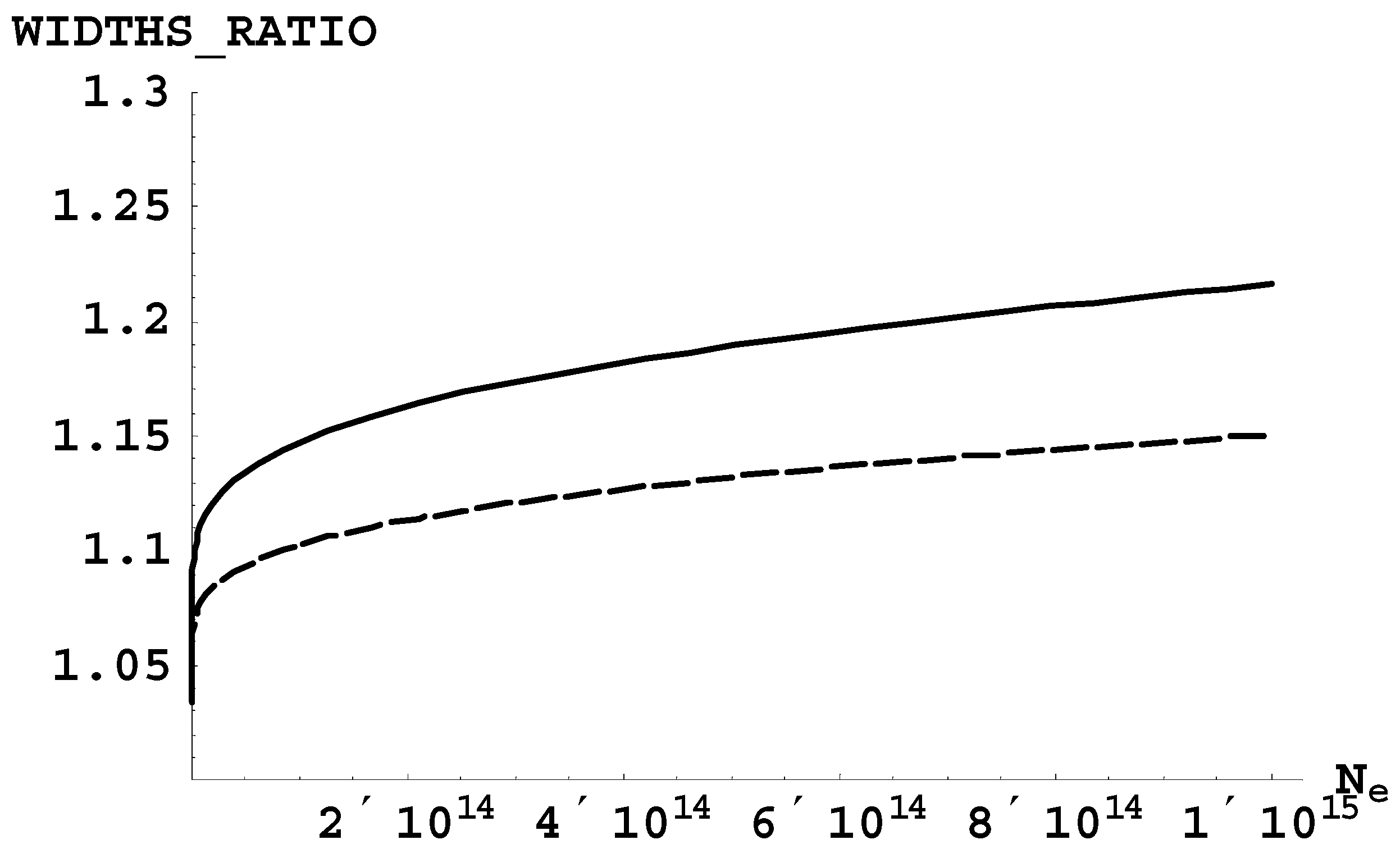
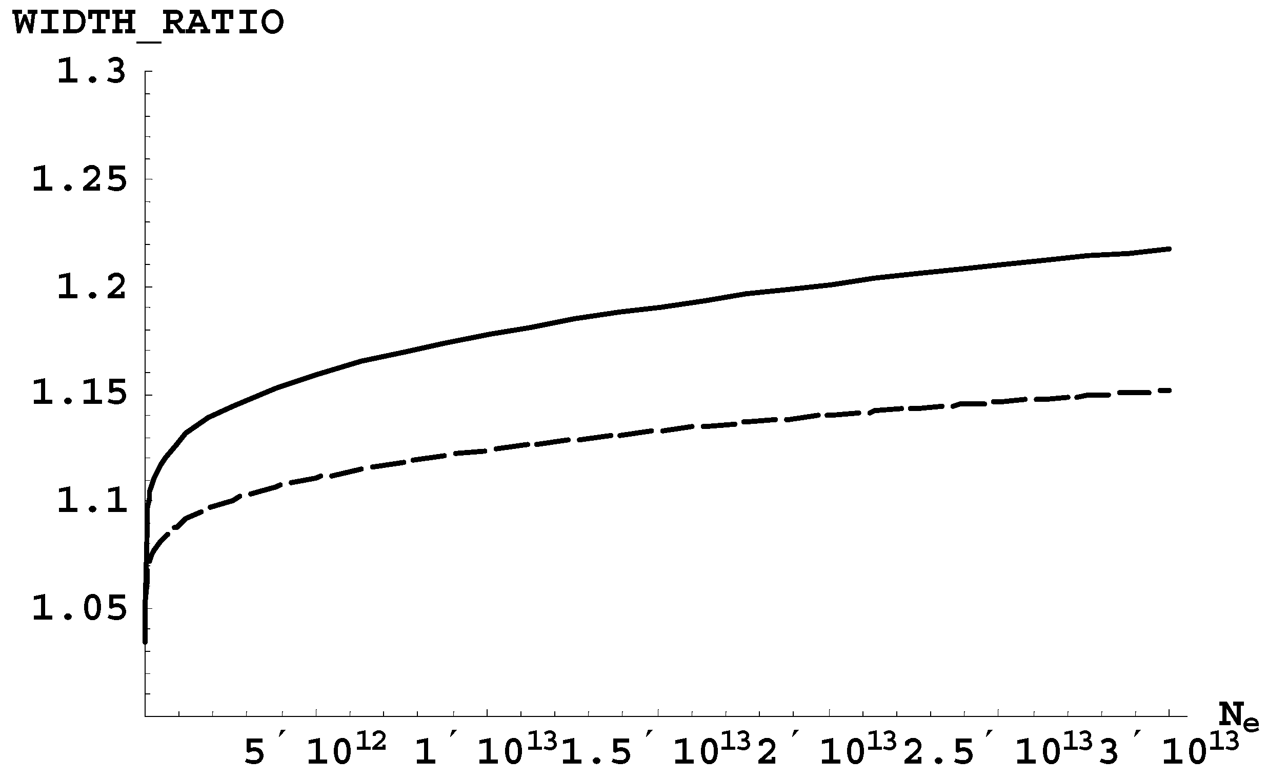
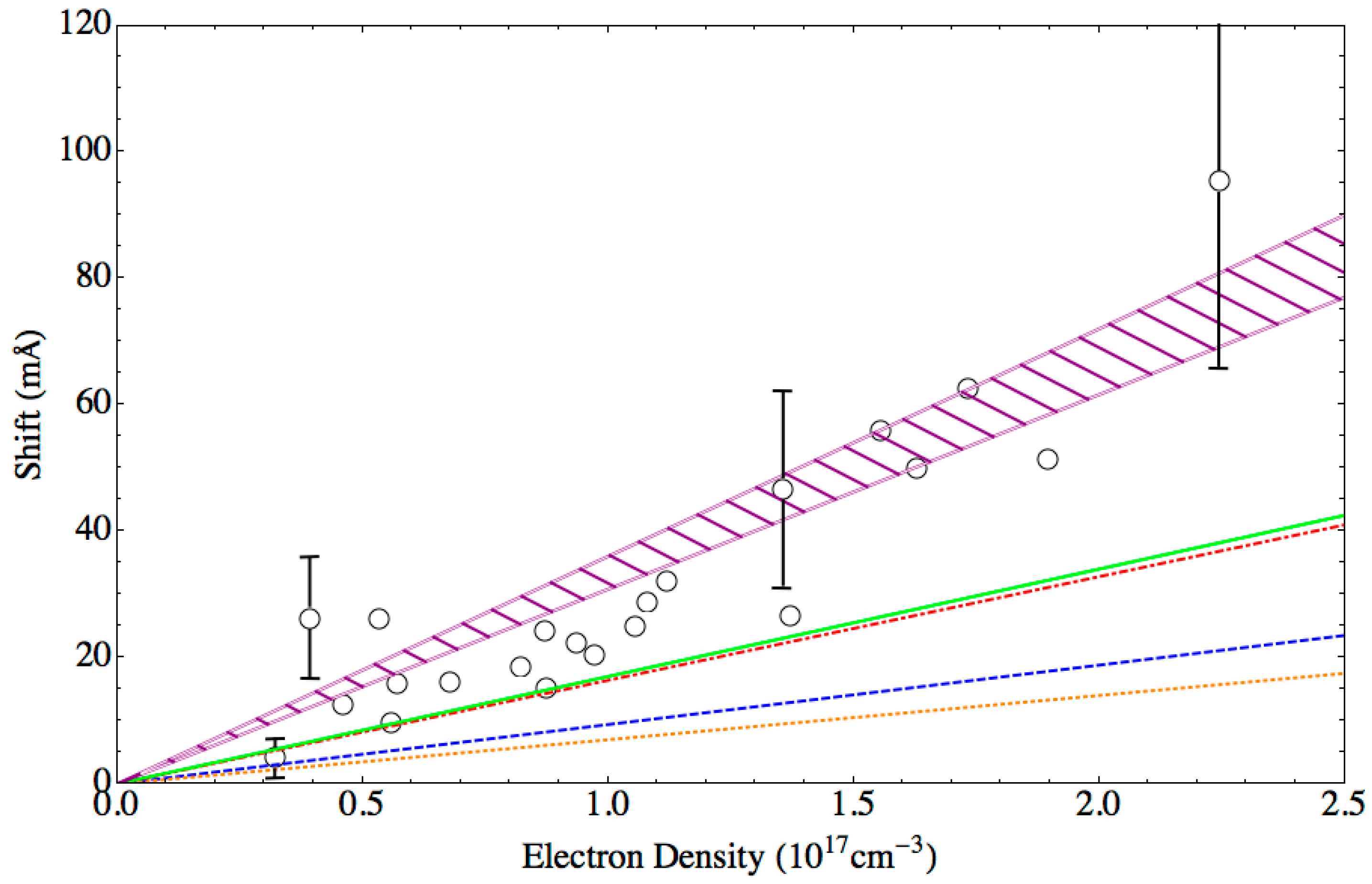
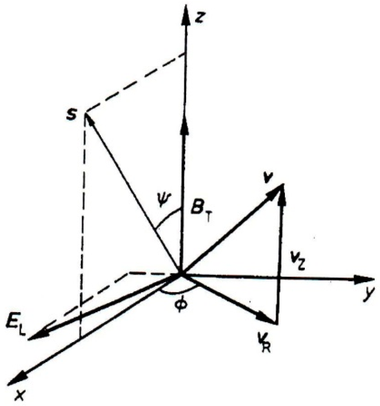
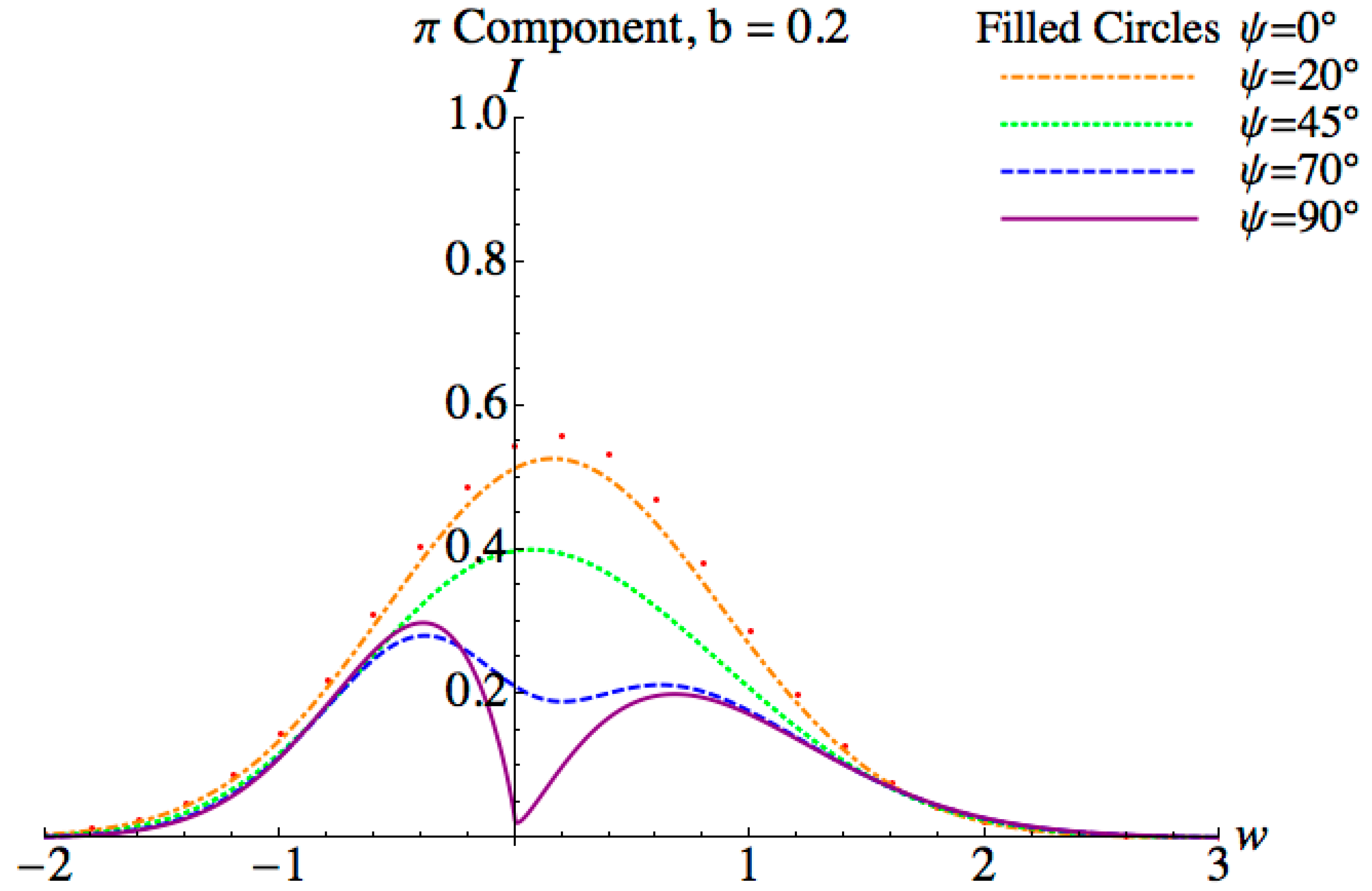
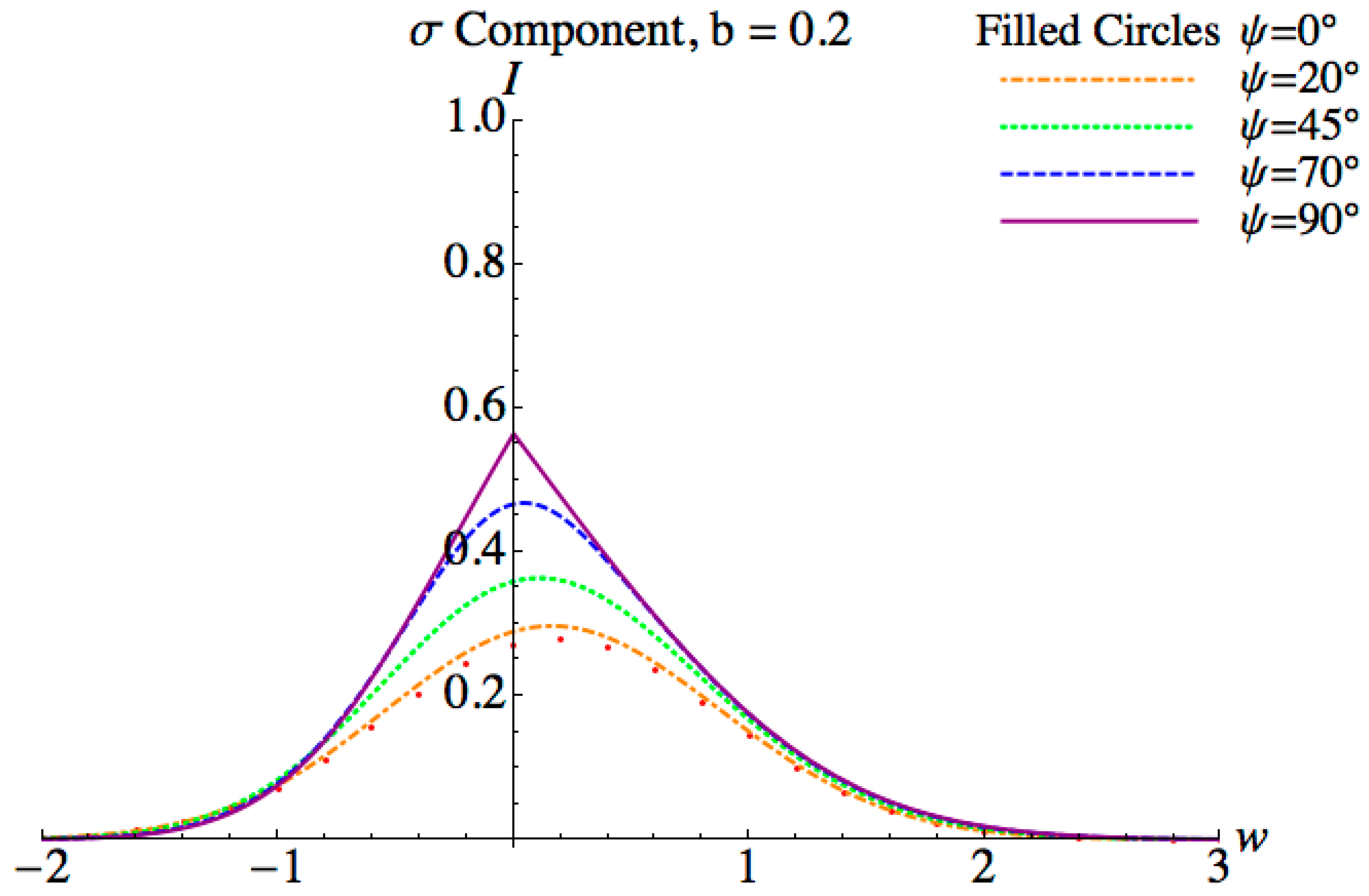
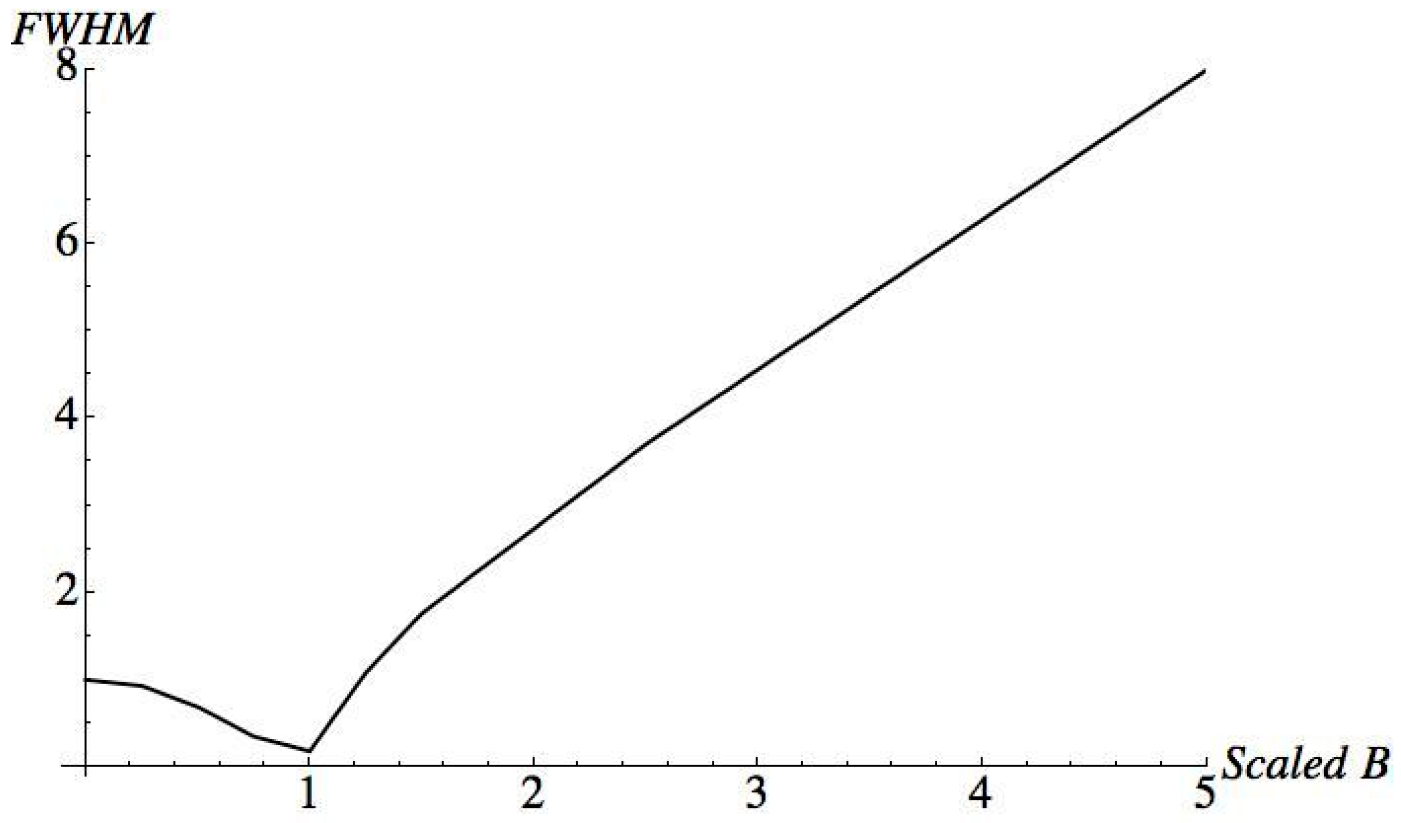
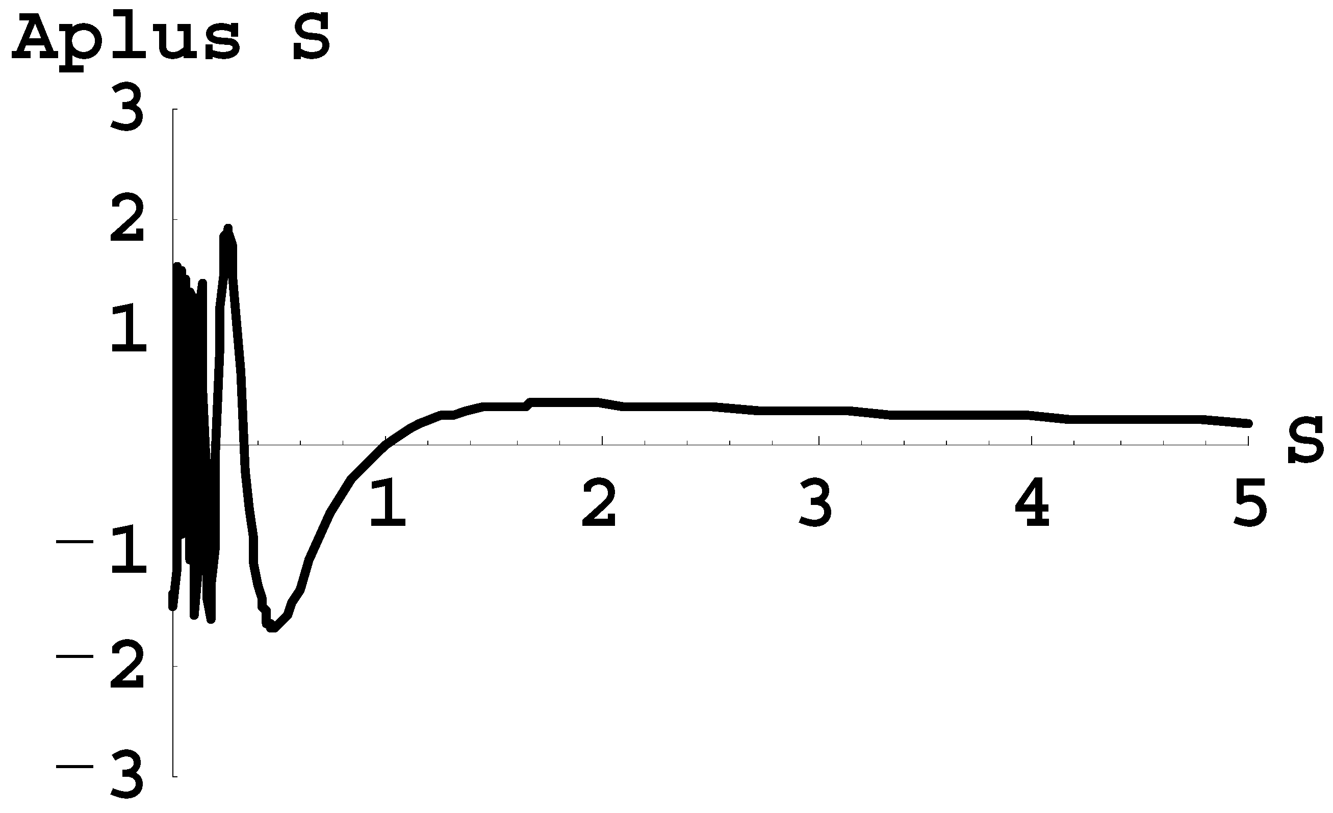
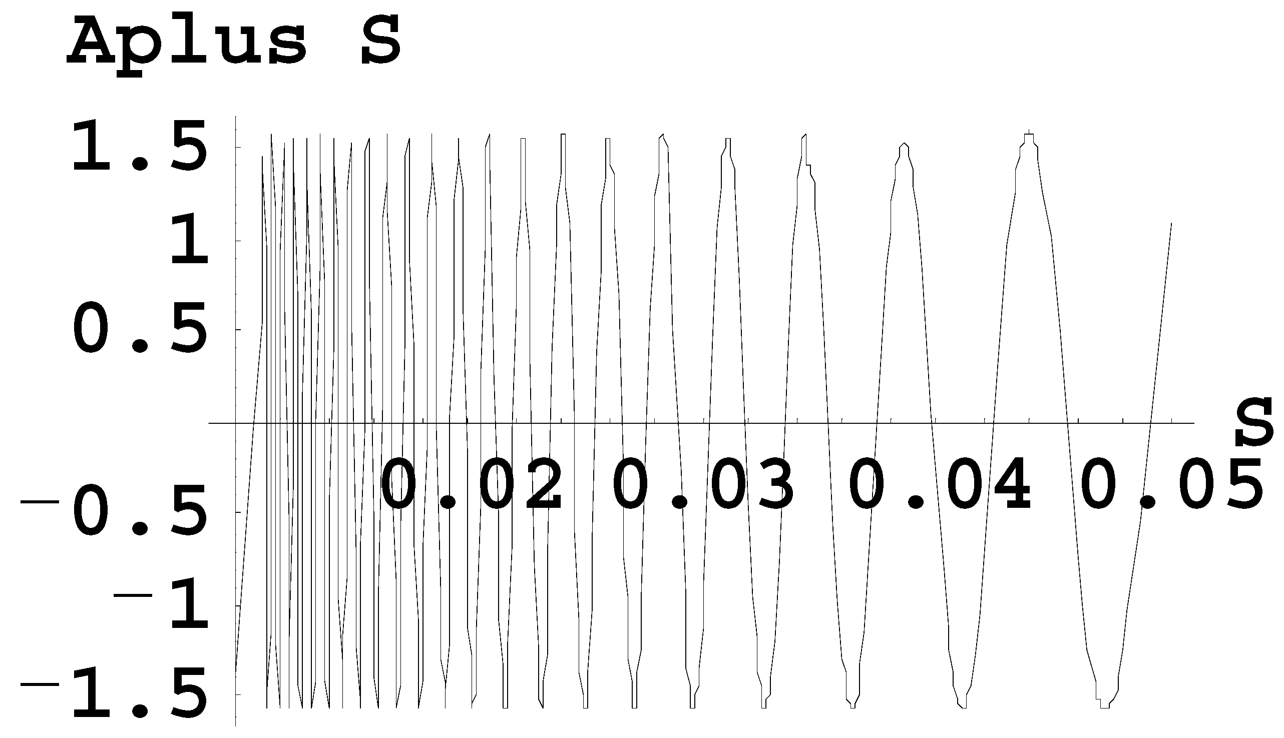
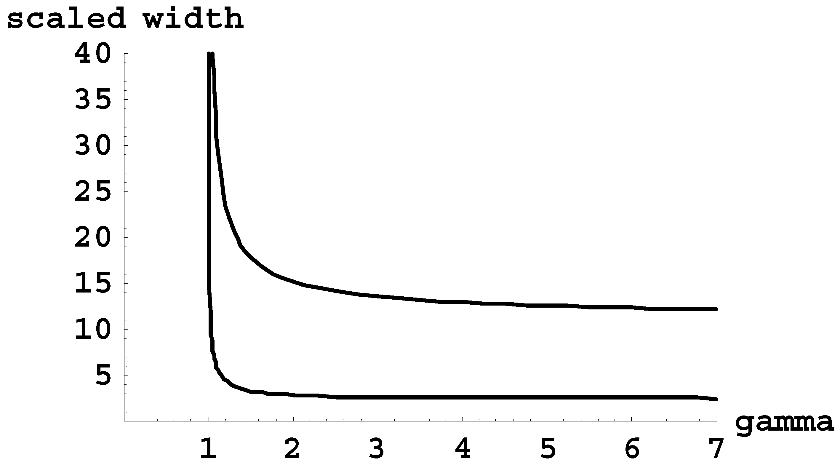
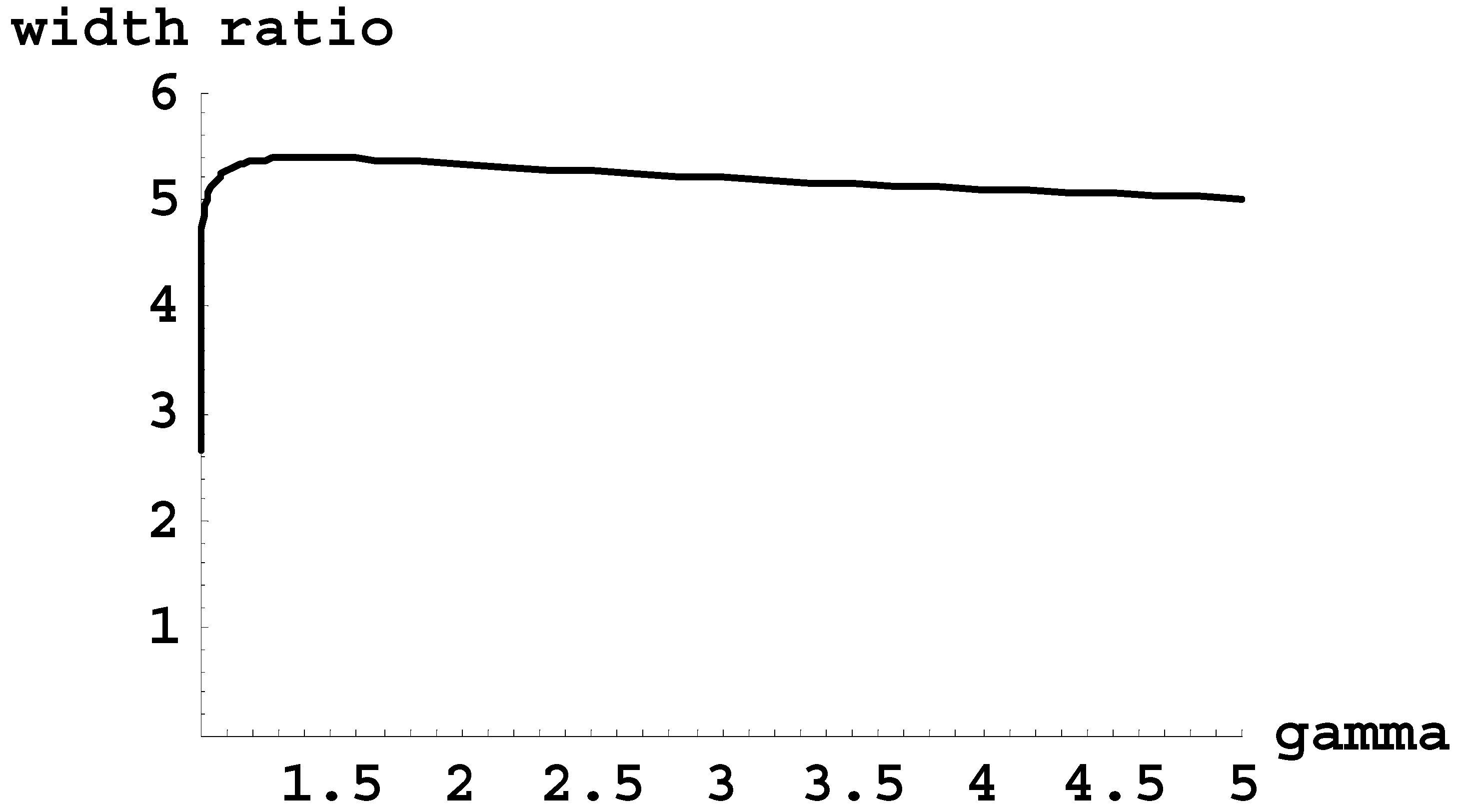
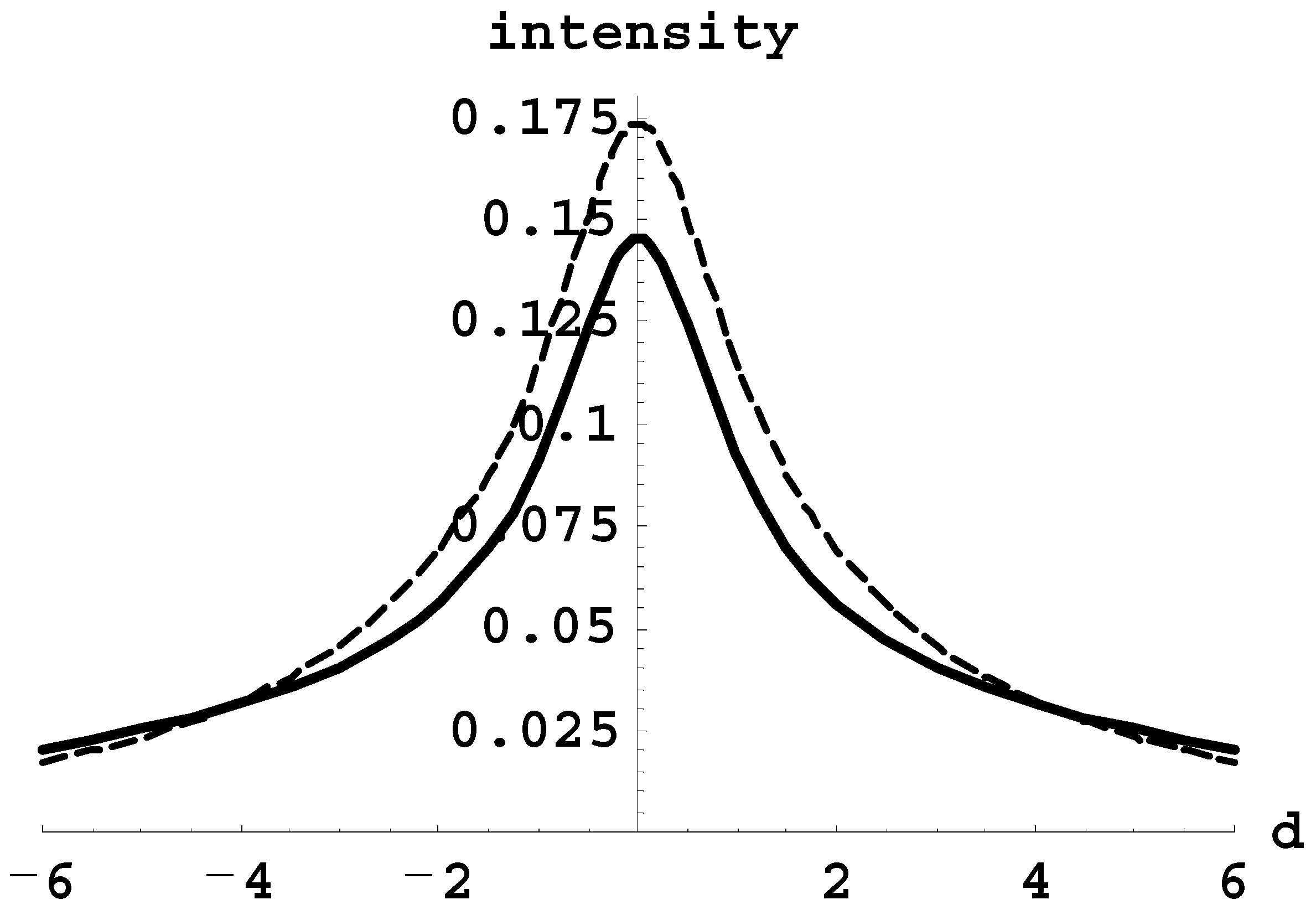
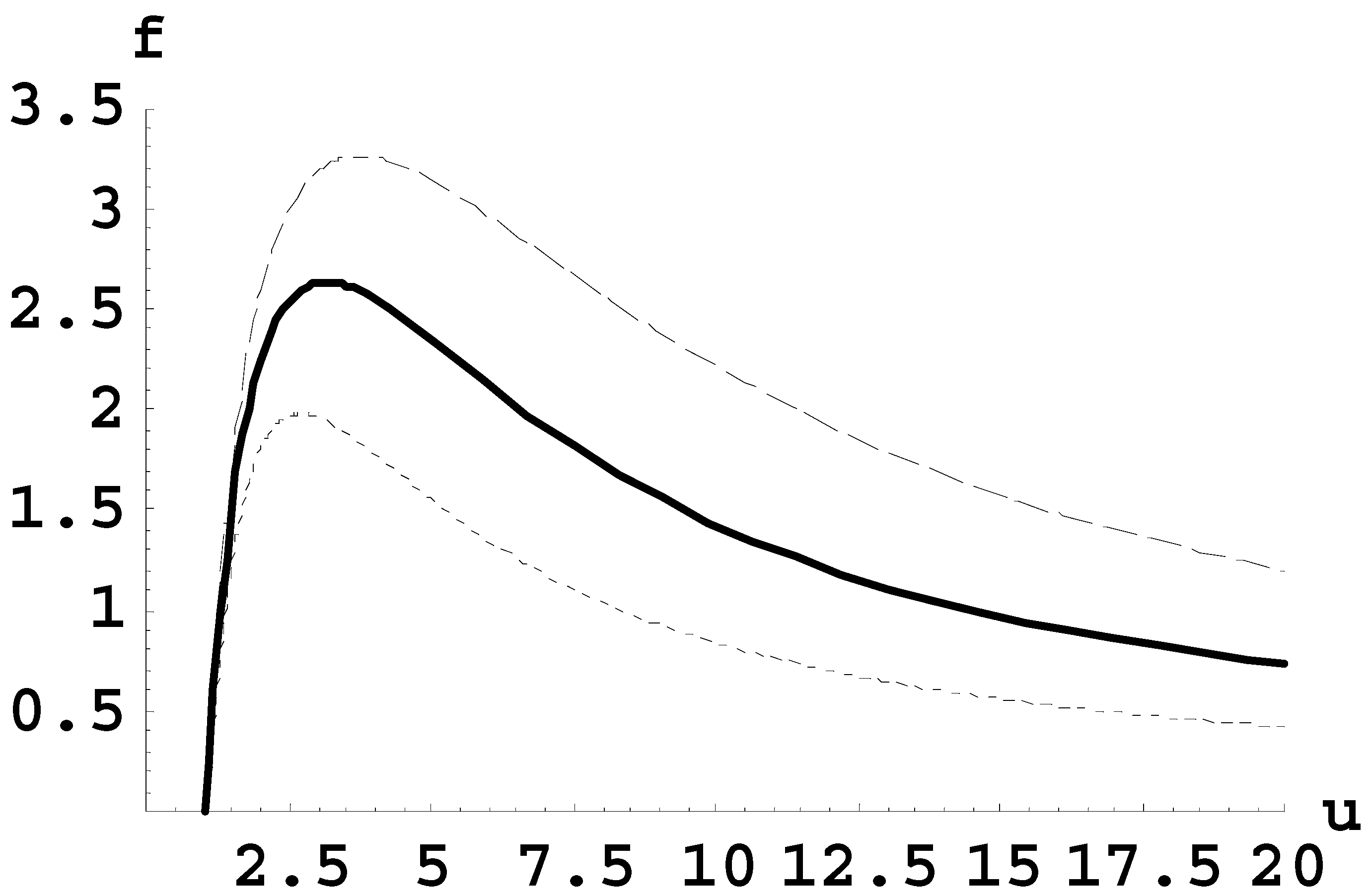
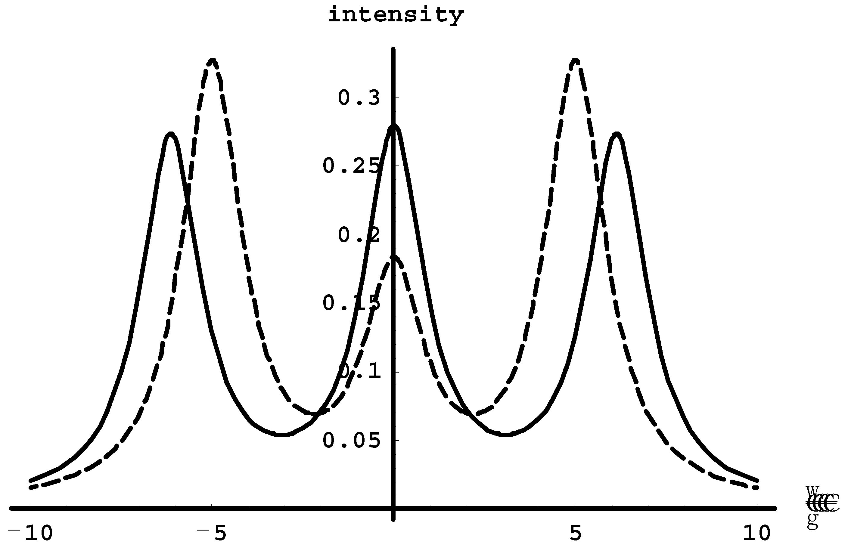
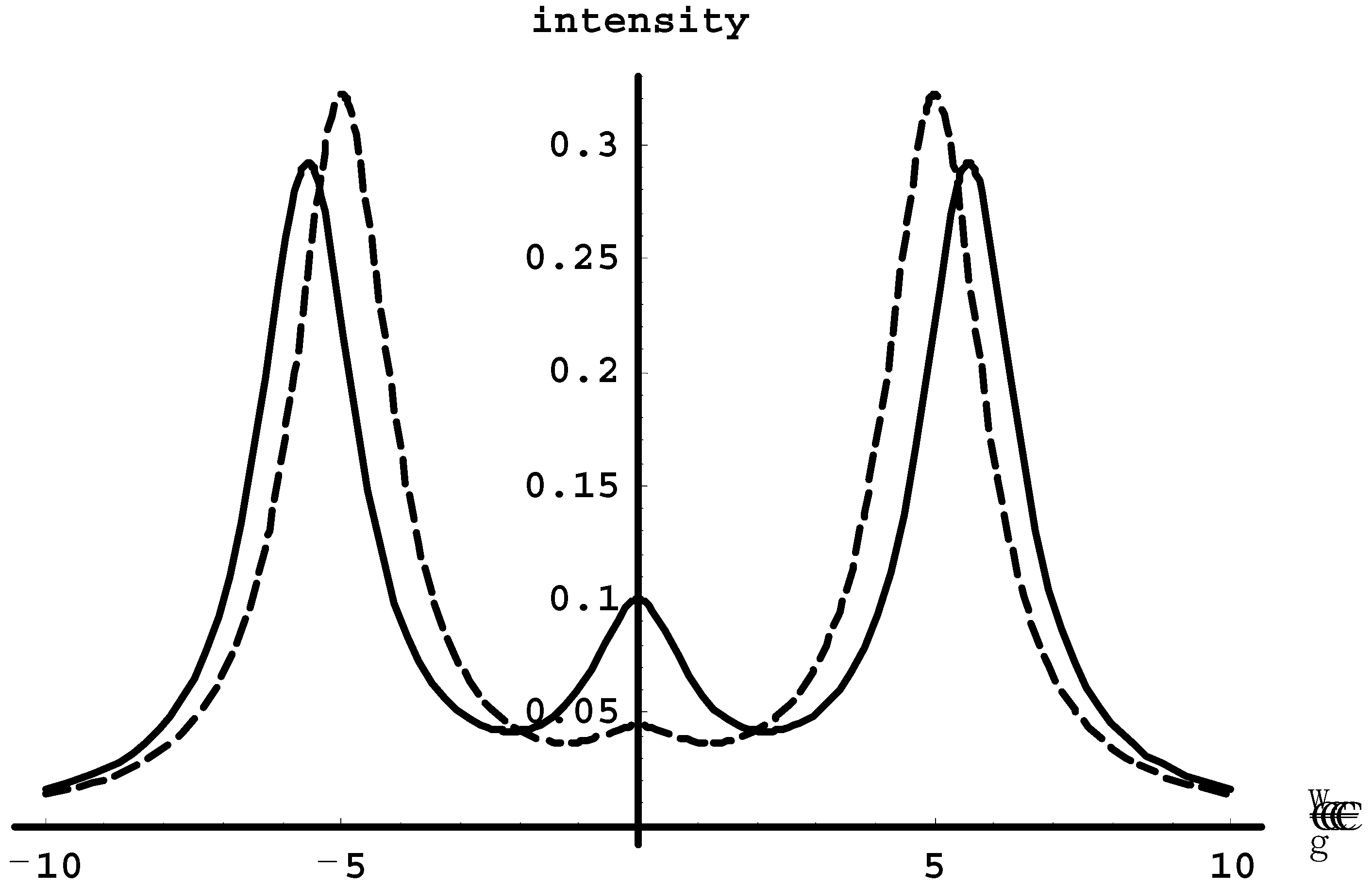
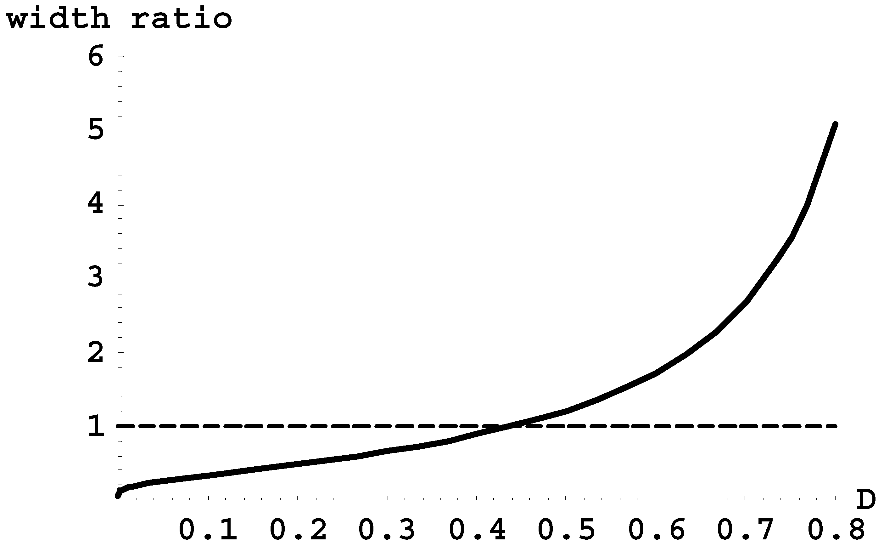
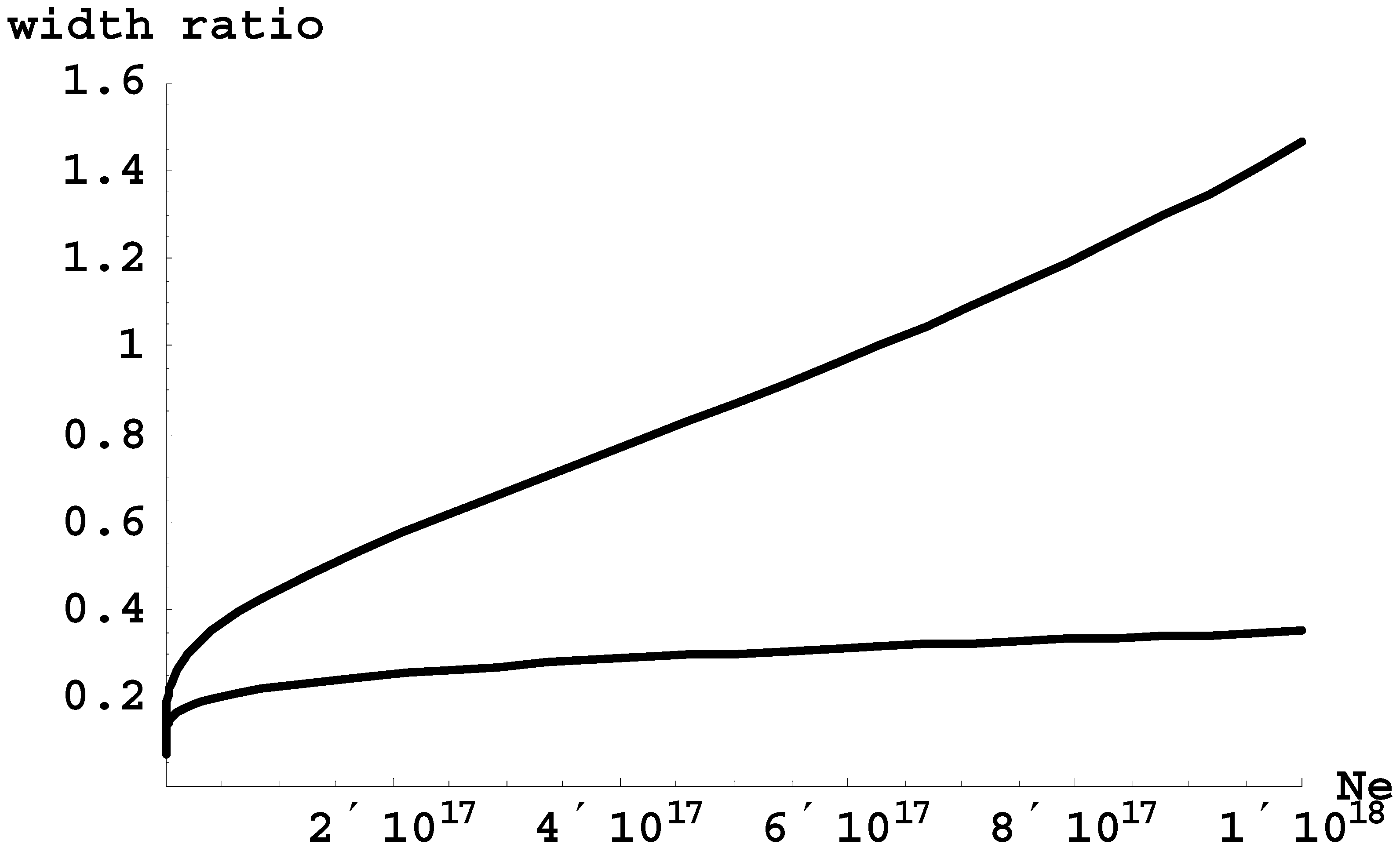
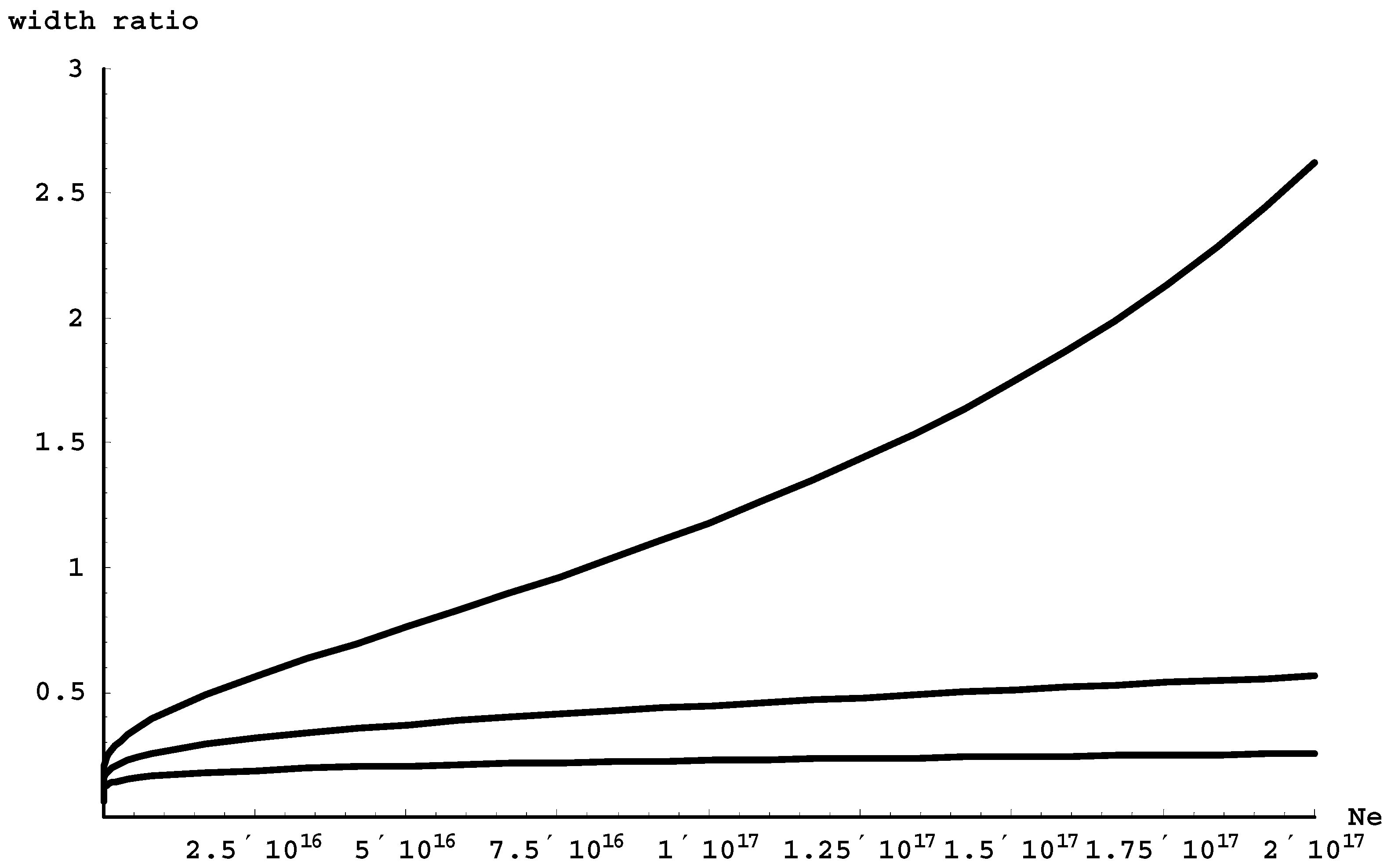
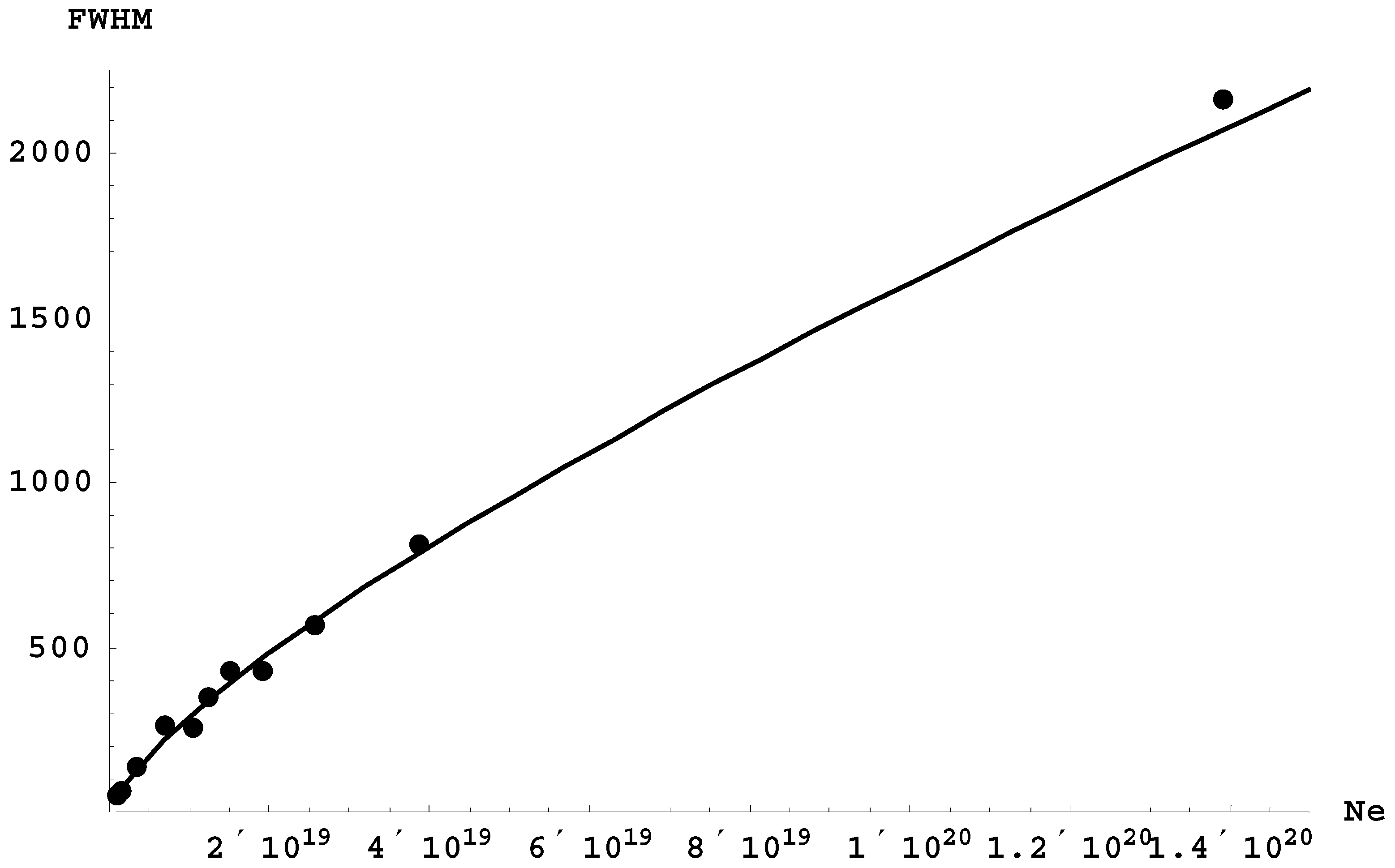
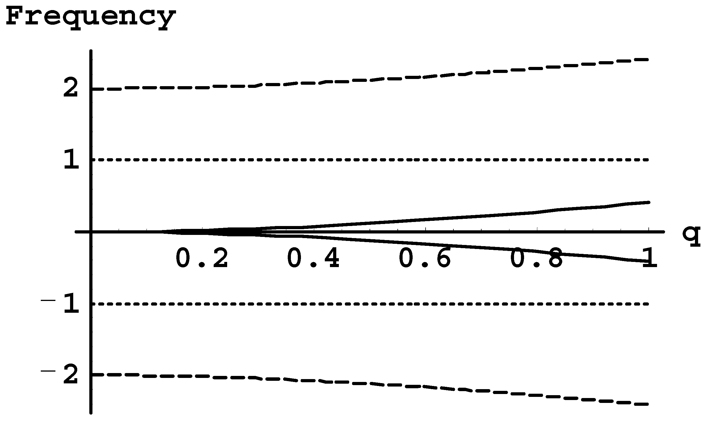
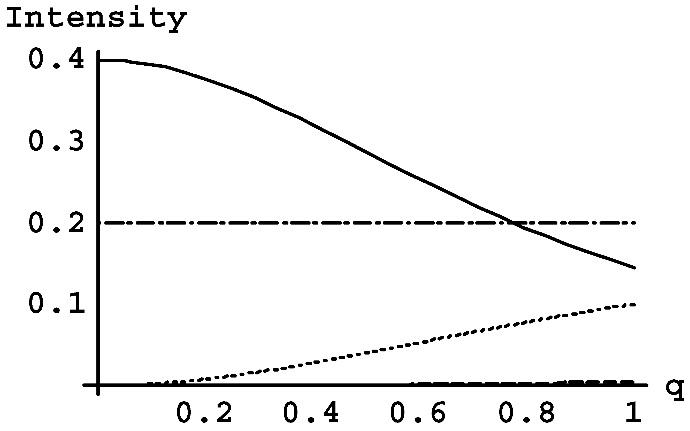
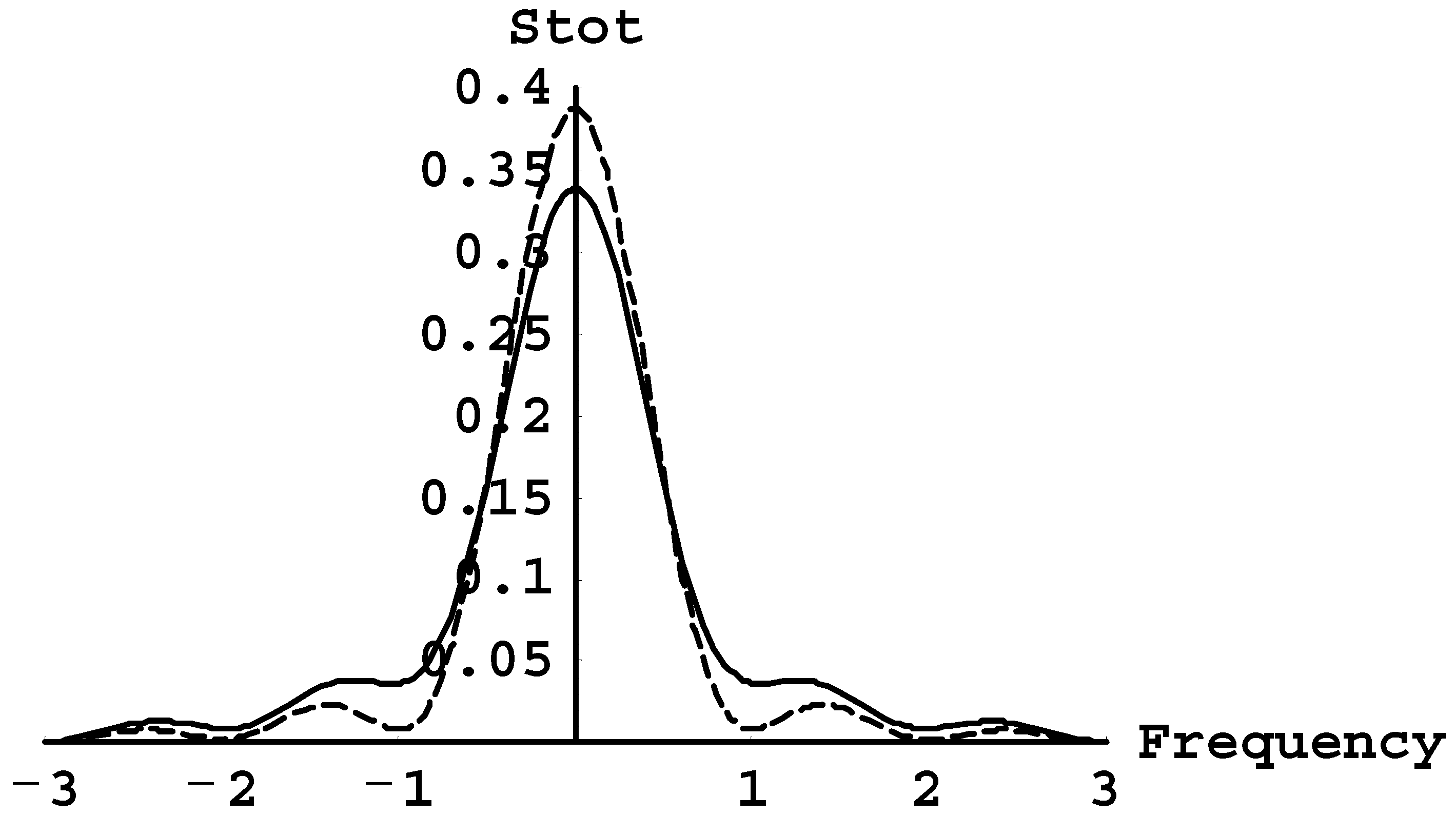
Table 1.
Ratio from Equation (2.13) for the Stark components of several Lyman lines of He II. at the temperature T = 8 eV and the electron density cm−3 [14].
Table 1.
Ratio from Equation (2.13) for the Stark components of several Lyman lines of He II. at the temperature T = 8 eV and the electron density cm−3 [14].
| n | |q| | Ratio |
|---|---|---|
| 2 | 1 | 0.3261 |
| 3 | 1 | 0.3748 |
| 3 | 2 | 0.7496 |
| 4 | 1 | 0.5156 |
| 4 | 2 | 1.0311 |
| 4 | 3 | 1.5467 |
Table 2.
Electronic shift Se of the hydrogen spectral lines H13–H17, as calculated by formulas from papers by Griem [41,43] and their comparison with the shifts from paper by Bengtson and Chester [34] observed in astrophysical (SSirius) and laboratory (Sexp) plasmas. All of the shifts are in Angstrom.
| n | λn(A) | Se(A) | SSirius(A) | Sexp(A) |
|---|---|---|---|---|
| 13 | 3734 | 0.0017 | 0.03 ± 0.03 | |
| 14 | 3722 | 0.0021 | 0.03 ± 0.05 | 0.00 ± 0.04 |
| 15 | 3712 | 0.0026 | 0.09 ± 0.07 | 0.15 ± 0.05 |
| 16 | 3704 | 0.0032 | −0.007 ± 0.05 | 0.00 ± 0.05 |
| 17 | 3697 | 0.0038 | 0.21 ± 0.08 | 0.30 ± 0.08 |
Table 3.
Shift Si,penetr due to penetrating ions [39] and its sum Stot with the electronic shift Se for the hydrogen spectral lines H13–H17, and the comparison with the shifts from paper by Bengtson and Chester [34] observed in astrophysical (SSirius) and laboratory (Sexp) plasmas. All of the shifts are in Angstrom.
| n | λn(A) | Se(A) | Si,penetr(A) | Stot(A) | SSirius(A) | Sexp(A) |
|---|---|---|---|---|---|---|
| 13 | 3734 | 0.0017 | 0.032 | 0.034 ± 0.010 | 0.03 ± 0.03 | |
| 14 | 3722 | 0.0021 | 0.043 | 0.045 ± 0.014 | 0.03 ± 0.05 | 0.00 ± 0.04 |
| 15 | 3712 | 0.0026 | 0.057 | 0.060 ± 0.018 | 0.09 ± 0.07 | 0.15 ± 0.05 |
| 16 | 3704 | 0.0032 | 0.073 | 0.076 ± 0.023 | −0.007 ± 0.05 | 0.00 ± 0.05 |
| 17 | 3697 | 0.0038 | 0.093 | 0.10 ± 0.03 | 0.21 ± 0.08 | 0.30 ± 0.08 |
Table 4.
The relative error in determining the electron density Ne from the experimental asymmetry degree while disregarding the contribution of the penetrating ions for the He II Balmer-alpha line. The physical quantities in Table 4 are explained in the text directly above Table 4.
| Ne,act/(1018cm−3) | ρact | ρquad | Ne,quad/(1018cm−3) | |Ne,quad − Ne,act|/Ne,act |
|---|---|---|---|---|
| 2 | 0.0925 | 0.0955 | 1.82 | 9.03% |
| 4 | 0.114 | 0.120 | 3.42 | 14.5% |
| 6 | 0.128 | 0.138 | 4.86 | 19.1% |
| 8 | 0.139 | 0.152 | 6.16 | 23.1% |
| 10 | 0.147 | 0.163 | 7.33 | 26.7% |
Table 5.
Central frequencies λj + k and relative intensities of components of the Ly-alpha line emitted by the inner electron. The central frequency is the frequency, at which the component has the primary maximum of the intensity for the zero eccentricity of the orbit of the outer, Rydberg electron. The frequencies are in units of the Kepler frequency Ω of the outer electron (given by Equation (12.3)) and they are counted from the unperturbed frequency of the spectral line. The sum of relative intensities of all the components is set to unity [150].
| Central frequency λj + k | ±[(1 + q2)1/2 − 1] | ±[(1 + q2)1/2 + 1] | ±1 | 0 |
| Relative intensity | [(1+q2)1/2 + 1]/[10(1 + q2)] | [(1 + q2)1/2 − 1]/[10(1 + q2)] | q2/[5(1 + q2)] | 1/5 |
© 2018 by the author. Licensee MDPI, Basel, Switzerland. This article is an open access article distributed under the terms and conditions of the Creative Commons Attribution (CC BY) license (http://creativecommons.org/licenses/by/4.0/).
Share and Cite
MDPI and ACS Style
Oks, E. Review of Recent Advances in the Analytical Theory of Stark Broadening of Hydrogenic Spectral Lines in Plasmas: Applications to Laboratory Discharges and Astrophysical Objects. Atoms 2018, 6, 50. https://doi.org/10.3390/atoms6030050
AMA Style
Oks E. Review of Recent Advances in the Analytical Theory of Stark Broadening of Hydrogenic Spectral Lines in Plasmas: Applications to Laboratory Discharges and Astrophysical Objects. Atoms. 2018; 6(3):50. https://doi.org/10.3390/atoms6030050
Chicago/Turabian StyleOks, Eugene. 2018. "Review of Recent Advances in the Analytical Theory of Stark Broadening of Hydrogenic Spectral Lines in Plasmas: Applications to Laboratory Discharges and Astrophysical Objects" Atoms 6, no. 3: 50. https://doi.org/10.3390/atoms6030050
Note that from the first issue of 2016, this journal uses article numbers instead of page numbers. See further details here.