1. Introduction
Many physical processes like the atom scattering on atom, molecule, surface, or a crystal and propagation of electromagnetic waves through a medium, are described generally by multidimensional integrals. The value of these integrals as a function of the parameters depends on the morphology of the phase of the integrand, where are the variables of integration.
The main contribution to the integral comes from the neighbourhood of the saddle points
, where
. For some parameters
a it is possible that some higher derivatives are equal to 0 at the saddle points, which causes coalescence of these points, increases the value of the integral that manifests itself as “rainbow and glory” [
1]. To analyze the rainbow phenomenon, it is important to know the caustic surface
, defined by the relation
.
By transforming the variables using a uniform one-to-one mapping, the phases can be transformed into simple forms, which are classified as seven “elementary catastrophes” [
2,
3]. There are four one-dimensional catastrophes: fold
, cusp
, swallow-tail
, butterfly
, and three two dimensional ones: hyperbolic umbilic
, elliptic umbilic
, parabolic umbilic
. The elementary Thom’s catastrophes in the context of the theory of atomic collisions have been discussed in detail by Connor [
4].
In the cuspoid case (one integration variable), the oscillatory integrals are usually written in the form:
where
a = {
a1,
a2, …} is a set of parameters. As
a varies, as many as
K + 1 (real or complex) critical points of the smooth, real-valued phase function
f can coalesce in clusters of two or more. The function
g has a smooth amplitude. In what follows we denote
. The critical (stationary) points
uj(
a), 1 ≤
j ≤
K + 1, are defined by
[
5].
In the case of a single real critical point the integral
is in the leading order approximated by [
6]:
where
and the subscript
q indicates a
quadratic expansion of
around
. The result is easily generalized to the case of
jmax (
) isolated real critical points [
7]. The main contribution to the integral comes from the regions around the stationary points
where the phase function
is slowly varying.
Since the positions of the critical points depend on
a, they can move close together and coalesce as
a varies. In the uniform asymptotic evaluation of oscillatory integrals the result is expressed in terms of certain
canonical integrals [
5,
7] and their derivatives. Each canonical integral is characterized by a given number of coalescing critical points. One defines a mapping
u(
a;
t) by relating
f(
a;
u) to the normal form of cuspoid catastrophes
in the following way:
with the
K + 1 functions
A(
a) and
b(
a) determined by the correspondence of
K + 1 critical points of
f and Φ
K.
In the simplest case of two coalescing critical points (K = 1, fold catastrophe) there is a single point where , i.e., the function has an extremum and there are two stationary points and . In some range of the parameter a the stationary points are real and . For the two points coalesce and . For other values of a the stationary points are complex conjugate solutions of Equation (2), i.e., .
The leading-order uniform approximation in the case of the fold catastrophe is given by [
8]
where
,
and
. The branches are chosen so that
is real and positive if the critical points are real, or real and negative if they are complex. (Note that
and in the case under consideration
).
The transitional approximation
reproduces the uniform approximation
on the neighbourhood of
(
) and enables analytical continuation from the region of real stationary points into the region of complex ones. The transitional approximation is given by [
9],
where
and
.
In order to obtain
A(
a) and
b(
a), a set of nonlinear equations has to be solved. These can be solved in principle, but there are practical difficulties in attempting a solution [
10]. On the other hand, away from
b = 0 the canonical integrals can be approximated in terms of canonical integrals
corresponding to lower-order catastrophes (i.e.,
J <
K) [
7,
10,
11,
12,
13,
14,
15,
16].
The motivation to study these types of integrals originates from the investigation of optical spectra of diatomic molecules [
9]. For example, in the semiclassical approximation the matrix element of the dipole moment
for the optical transition is proportional to the integral [
11]
The radial movement of atoms is described classically,
. The phase function in the integral (6) is
, where
is the energy difference of the upper and lower electronic state energies. The condition
gives the saddle points which satisfy the classical Franck–Condon condition
. If there are points
satisfying the condition
, the method suggested in
Section 2 of this paper is a good choice to calculate the integral in Equation (6).
In the following sections we propose a new procedure for the approximate evaluation of oscillatory integrals with several stationary points.
2. A New Procedure for Approximate Evaluation of Oscillatory Integrals
Let there be a point
in the integration interval
which satisfies the condition
. In the neighbourhood of this point one defines a function:
The first derivative of this function, , has an inflection at the point . If , is monotonic function. In the case when , the function has two extremes at real points .
If there are
m points
,
, satisfying
and
, these points divide the interval
into
m + 1 intervals
and the integral
can be written:
where the end points of the integration
and
(
and
have been introduced. At each interval
the function
has a simple property. If
, the function
is monotonic on the interval
and has a single real saddle point. In the case
there is a point
,
and the function
has an extreme at
and two saddle points.
One defines a function as a series expansion of the phase around up to the quadratic term: . Note that , , , and .
We define the integral
, which has an exact solution
Relation (8) can be written as:
By combining integrals in the first three sums a simple expression is obtained:
where integrals
are
The functions
and
are shown in
Table 1.
The relation (10) can be generalized to be valid for the case
as well:
So far, no approximation has been made. The relation (10) is an identity. An integral of the function, the phase of which has several real stationary points, is divided into the sum of the integrals whose phase functions have either one or at most two stationary points.
If the phase function has only one real saddle point and its first derivative is monotonic, the value of integral can be calculated using Equation (2). In the case when the function has a single extreme at the point and two real or complex saddle points, the integral is easily soluble using the approximate methods described in the introduction (Equation (4)). If the phase is given by numerical points in the region where a complex pair of saddle points contributes to the integral, the analytical continuation of (5) can be used. The numerical accuracy of this method is determined by the accuracy of the leading-order uniform approximations (2) and (4).
3. Results
The method outlined in
Section 2 was tested on three examples that are typical for the spectra of diatomic molecules. For simplicity we use the phase function given by the polynomial phase of the Thom’s elementary catastrophe. The case when
and the difference potential
are both monotonic functions with a single inflection point is illustrated by the analysis of the Pearcey integral
in
Section 3.1.1. In
Section 3.1.2 with the Pearcey integral
we analyze the case when the function
and the difference potential
have two extremes and one inflection point. Finally, in
Section 3.2 we illustrate the case when the difference potential has an extreme near the turning point by the analyses of the swallow-tail catastrophe integral
. For simplicity, we take
in all the examples. The dependence of the integral (6) on the variable transition dipole moment was discussed by Beuc et al. in [
9].
3.1. Cusp Catastrophe (K = 2)
Let us consider the Pearcey integral, the canonical integral for the cusp catastrophe (
):
(Other notations also appear in the literature). The Pearcey integral is symmetrical with respect to variable y:
. For the numerical integration of the Pearcey integral we used the form:
[
13]. The numerical evaluation of the integral and all other calculations in this paper were done using the Wolfram Mathematica 11.3 computing system.
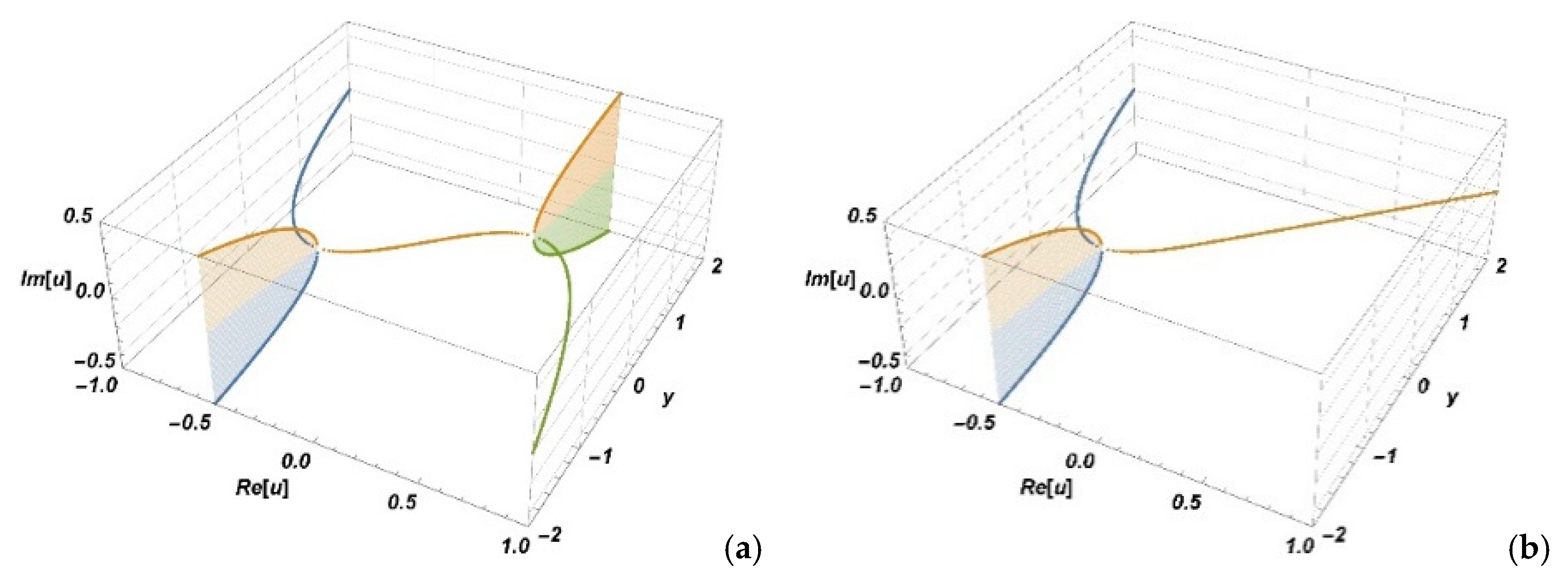
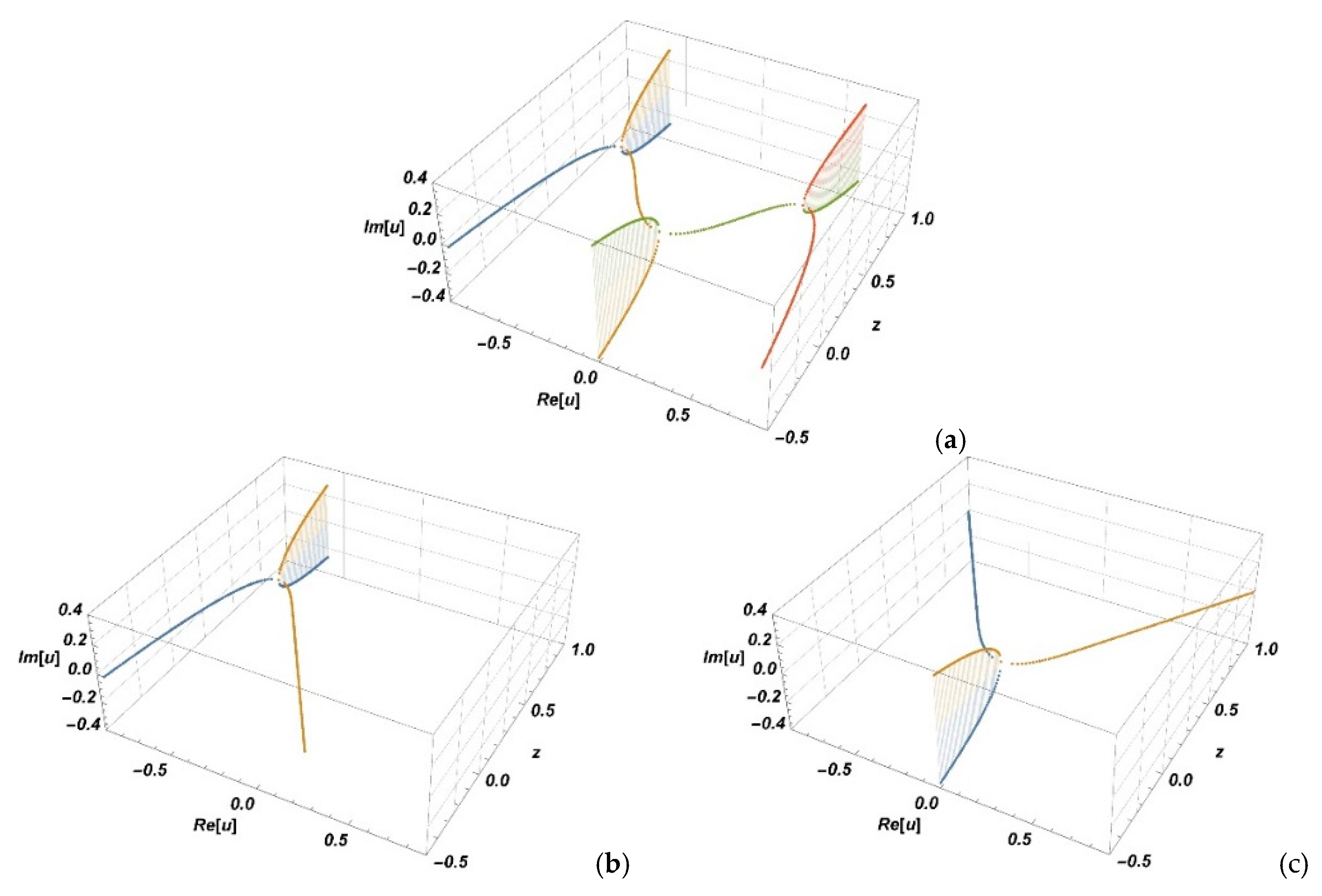
The phase function in (6) is
. There are three saddle points defined by the condition
(
Figure 1 and Figure 3a):
where
and
. If
δ < 0, all saddle points are real and if
δ > 0, one saddle point is real and the other two are complex conjugates of each other (
Figure 1 and Figure 3a). There are two bifurcation points
defined by the relation
. There is a single point
where
and
, i.e.,
. In the special case
one has
.
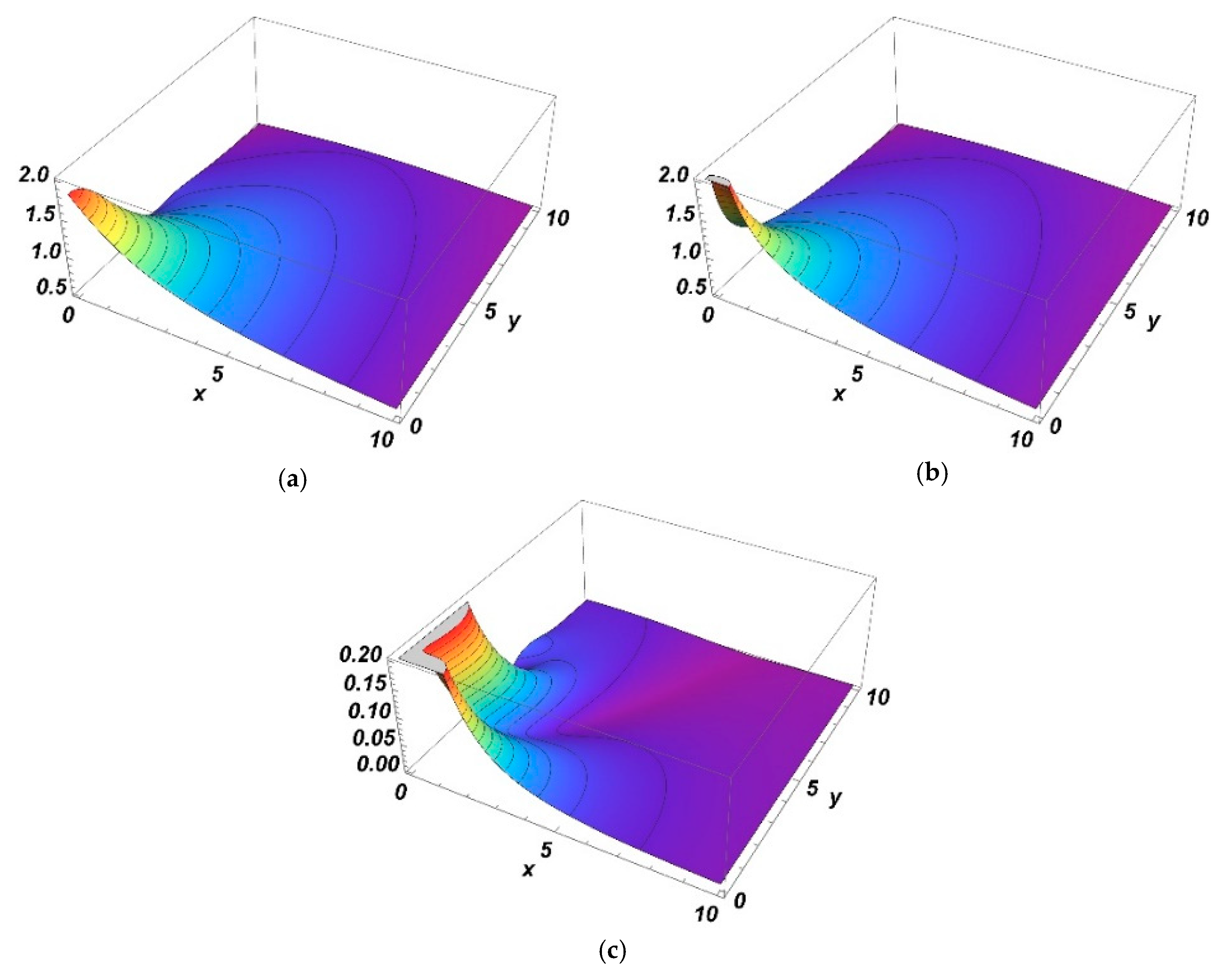
3.1.1. Case
If
, then
δ is always positive, the saddle point
is real and the points
and
are complex conjugates (
Figure 1).
The function
is monotonic and, according to Equation (2), the value of the Pearcey integral can be approximated as
From
Figure 2 and
Table 2, we can freely estimate that the difference of the approximation
and the exact values of
is smaller than few percent if the condition
is satisfied.
3.1.2. Case
According to
Section 2, when
using the relation (10) the Pearcy integral can be written as:
Here the phase functions have the form
,
,
. It is easy to show that
,
, and the Pearcey integral can be decomposed exactly as
The function
has on the interval
only one bifurcation point
, where
, and two saddle points
,
(
Figure 3b).
Using relation (4), the integral
can be approximated as:
where,
,
.
We define the Airy approximation of the Pearcey integral as:
Paris obtained the asymptotic form of
P(
x,
y) by considering its analytic continuation to arbitrary complex variables
x and
y [
15]. In
Table 3. we compare some values of
P(
x,
y) for large negative values of
x when
y = 2 and 4 to the asymptotic values [
15] and the present work.
Kaminski [
16] rewrites (8) as a sum of two contour integrals, one of which has exactly two relevant coalescing saddle points. This allows him to apply a cubic transformation introduced by Chester, Friedman, and Ursell [
17] and to construct a uniform asymptotic expansion of (7) as
x → −∞ with
δ varying in an interval containing 0. The leading-order approximation was already given by Connor [
12] and Connor and Farrelly [
13]. In
Table 4 the values of
are compared to Kaminski’s results [
16] and the approximation
at some points on the caustic
.
From
Table 3 and
Table 4, and
Figure 4, we estimate that the difference of the approximation
and the exact values of
is smaller than a few percent if the condition
is satisfied.
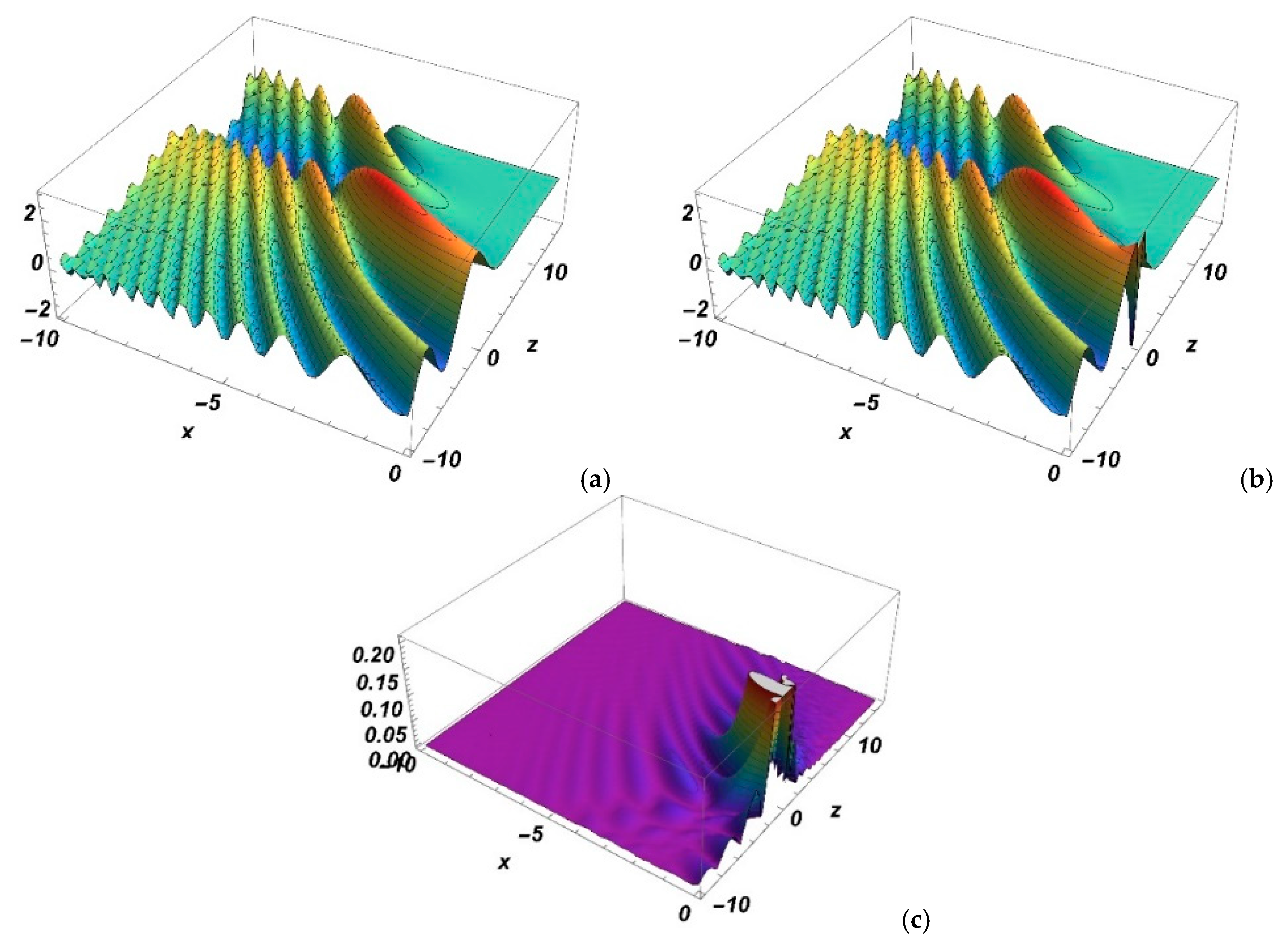
3.2. Swallow-Tail Catastrophe (K = 3)
The swallow-tail canonical integral is defined by:
As a further example, we consider a special case of the swallow-tail integral, i.e.,
—the oddoid integral of the order two [
18]. For the real
x and
y the function
is also real, and for the numerical evaluation the equation
is used. This integral is of interest in the study of bound-continuum [
19] and bound-bound [
20] Franck–Condon factors. The analysis is applied to the domain
.
In that case the phase function is
and it is antisymmetric with respect to the variable
u:
. There are four saddle points
defined by the condition
:
The condition
defines three real bifurcation points
of the “fold” type:
,
. As there are two real points (
,
) satisfying the conditions
and
, according to
Section 2, the integral
can be written as:
where,
Since
, it follows that
and
. Also,
,
, and
. Using Equation (9) to calculate
, one can write Equation (22) in the form:
This expression exactly represents the function . To find an approximate solution of the integral one needs to calculate integrals and , using the approximation described by Equation (4).
The function
has two saddle points (see
Figure 5b):
,
. Applying Equation (4) one gets,
where
and
.
The function
has two symmetrical saddle points:
,
(
Figure 5c). Since
and
, the approximation of the integral
has a simple form,
where
.
Finally, we write the approximation of the integral
as:
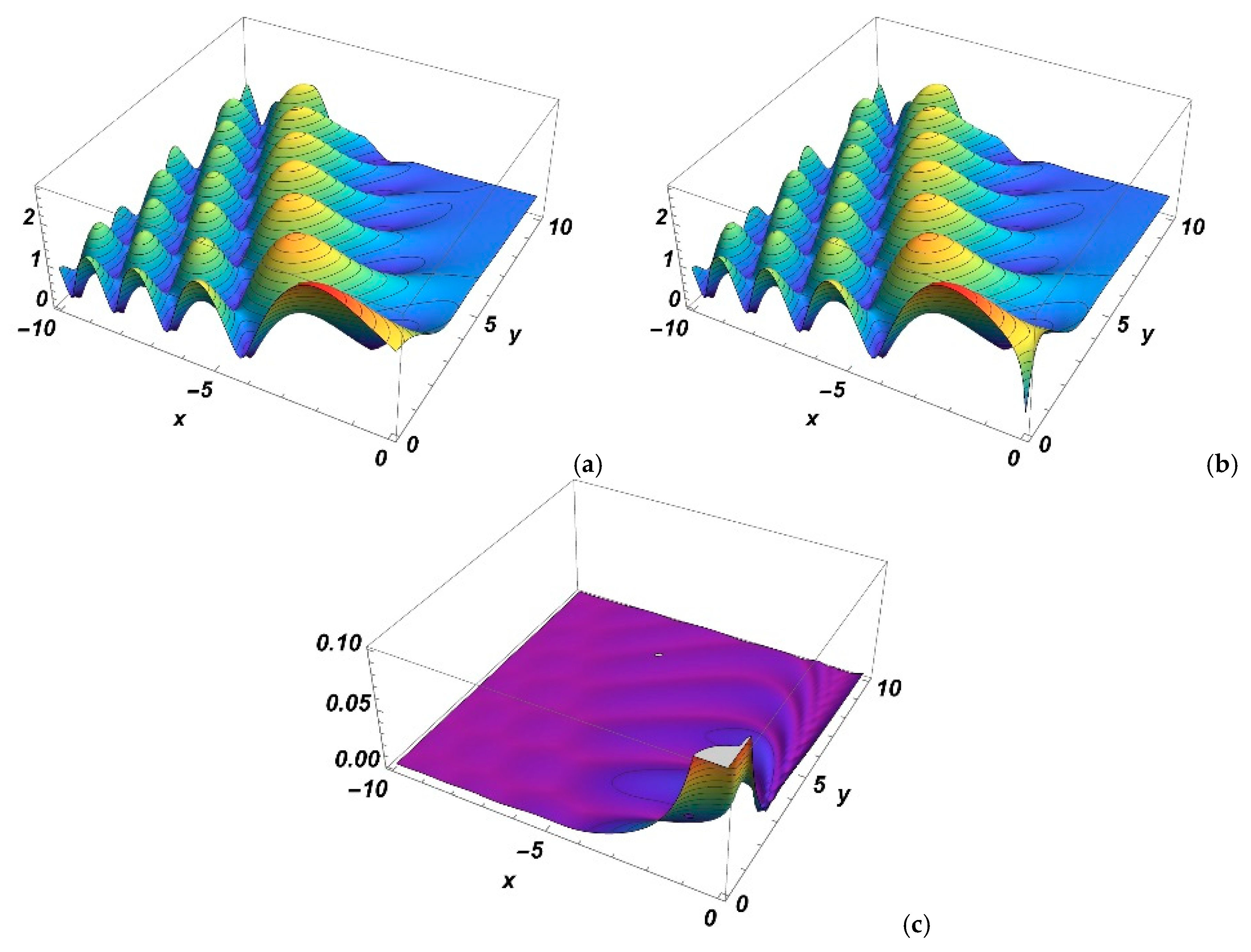
In
Table 5 we compare the values of the functions
and
at the caustics i.e., at the points where the function
has an extreme. These comparisons together with the comparison of functions in
Figure 6 clearly show that the function
is a good approximation of the function
if the condition
is satisfied.


