Line Shapes in a Magnetic Field: Trajectory Modifications I: Electrons


Hellenic Army Academy, Varis—Koropiou Avenue Vari P.O. Box 16673, Greece
Atoms 2019, 7(2), 52; https://doi.org/10.3390/atoms7020052
Submission received: 15 February 2019
/
Revised: 21 May 2019
/
Accepted: 22 May 2019
/
Published: 27 May 2019
(This article belongs to the Special Issue Plasma Spectroscopy in the Presence of Magnetic Fields)
Abstract
:In recent work, the effect of a magnetic field on the line shapes via the modification of electron perturber trajectories was considered. In the present paper we revisit this idea using a variation of the Collision-time Statistics method, in order to account for relevant perturbers. We also obtain line profiles for the hydrogen line for conditions of astrophysical interest. Although the Collision-time statistics method works for both electrons and ions, we apply a simplification here that results in an excessive number of ions having to be simulated. As a result, the present, simplified version, is typically only appropriate for electrons.
1. Introduction
Line shapes in random media, such as a plasma, are broadened and possibly shifted due to the interaction with the random fields of the medium. The presence of an additional field in the medium, such as an electric field for instance due to a laser, or a magnetic field, has three effects: First, it dresses the random interaction, resulting in lineshape modification. This normally narrows the lines, but can also result in satellite merging and hence line broadening compared to the no external field case. Second, it may modify the distribution functions of the medium particles. Third, it may modify the motion, for instance trajectories or equivalently dielectric properties of the medium. It is the purpose of this work to investigate this last effect, and for this reason we keep other factors, such as the shielding length and distribution functions unchanged by the magnetic field. It is not the purpose of this paper to include all or even the most relevant effects (for example, ion broadening would normally be dominant for tokamak conditions), but to isolate and investigate the effect of spiralling electron trajectories as suggested in a recent paper [1], keeping all other things standard. For example, we do not discuss whether quantum effects are enhanced or diminished in importance due to the smaller effective velcocities or larger radii. We limit ourselves to electrons in the present work for reasons that will be explained later.
2. Theoretical Formulation
We make the following assumptions in calculating the effects of the spiral orbits on the line shapes in order to the effect of spiralling trajectories and to make contact and comparisons with previous work cited [1] that also made these assumptions:
- The distribution functions, e.g., the Maxwellian velocity distribution is affected by the B-field. It has been known for a long time that the low frequency component of the electric microfield (and thus the impact parameter or initial particle position distributions) is unaffected by a magnetic field in a thermal plasma [2], but this is not the case here.
- The shielding is also not affected, e.g., Debye screening. In principle, since shielding is provided by the motion/rearrangement of plasma electrons and ions, any field that affects their motion will also affect shielding. As discussed above, however, normal Debye shielding is assumed.
2.1. Collision-Time Statistics
To include and only the relevant perturbers, we use a modification of the collision-time statistics method of Hegerfeld and Kesting [3] with Seidel’s improvement [4]—see Reference [5] for details. This was also suggested in the context of preliminary calculations for the same effect discussed here—“One major issue is the design of numerical simulation techniques which are suitable for addressing the electrons in near-impact regime within a reasonable CPU time.” [6].
We start by introducing , which is the maximum time for which we need to compute the autocorrelation function C(t), i.e., the Fourier transform of the line profile, which decays with time. It may be a few times the inverse HWHM, but it could also be much shorter than that, if an asymptotic form is realized before then. Next, we define as “relevant” perturbers those that come closer to the emitter than a distance , defined so that the interaction is negligible for distances larger than during the interval (0,). For a Debye interaction, we usually take , where denotes the shielding(Debye) length. This is because the interation becomes negligible ( for larger distances).
In this work we consider a neutral emitter at the origin of the coordinate system. With these assumptions, perturbers move in a helical path characterized by the parallel constant velocity , where the magnetic field direction defines the z-axis (passing through the emitter), the perpendicular velocity with magnitude and impact parameter , which is the distance of the center of the spiral to the z-axis, i.e., the perpendicular motion is a circular motion with the Larmor radius around the center , with the cyclotron frequency and Q the perturber charge.
The z-coordinate of the trajectory is
with
with the times of closest approach representing the time the perturber trajectory intersects the x-y plane and being uniformly distributed. thus represents how far from the x-y plane the perturber is at .
The perpendicular component is:
As discussed above, the relevant perturbers must come closer than :
for at least one time in the simulation interval [0,].
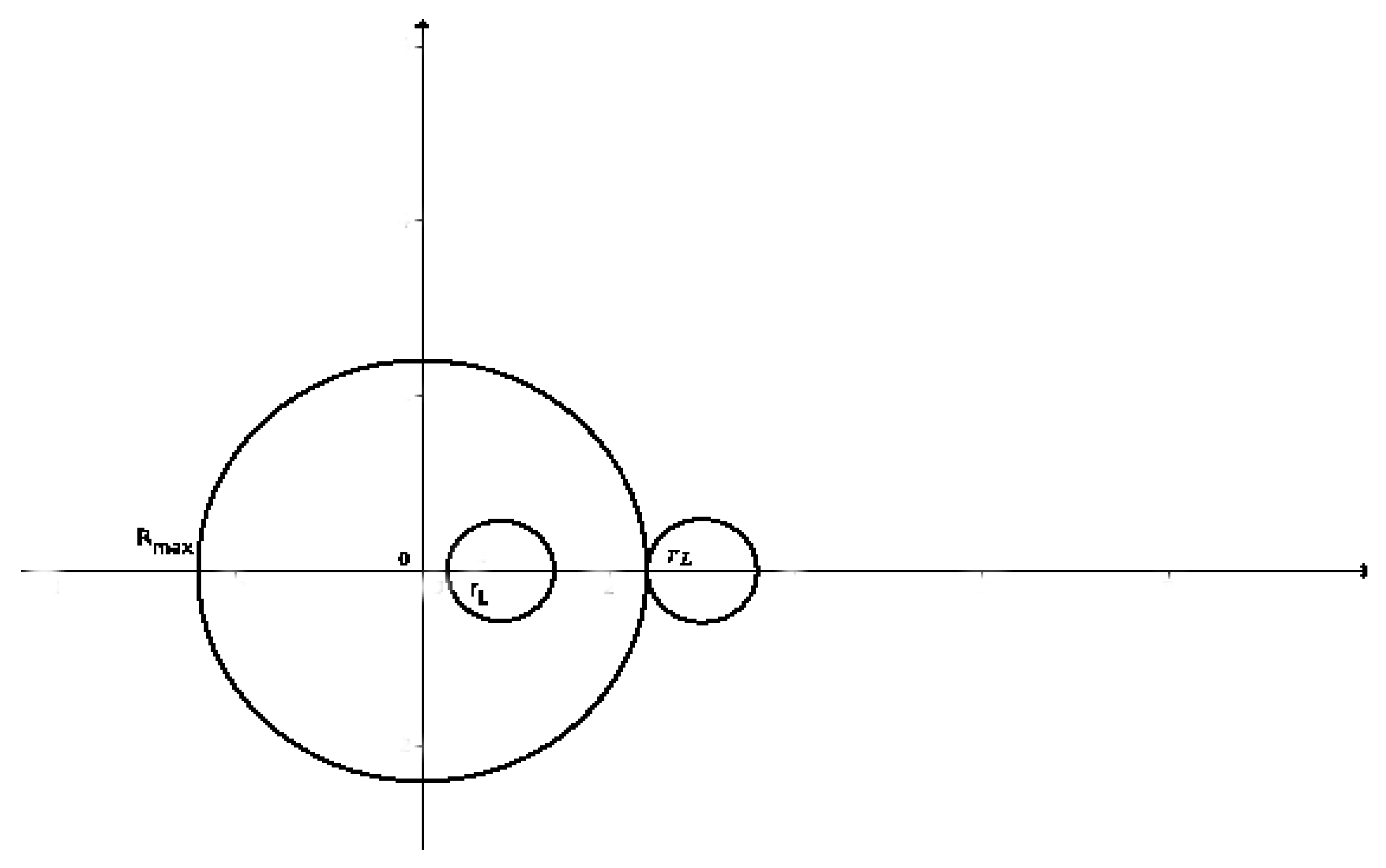
We consider two cases: The case is depicted in Figure 1: Relevant are in . Note that a larger cylinder radius and hence more perturbers contribute than in the case without magnetic field; however, these extra perturbers in () as well as the perturbers in () . Note that this is the only case considered in [1].1
2.2. Cylinder Radius
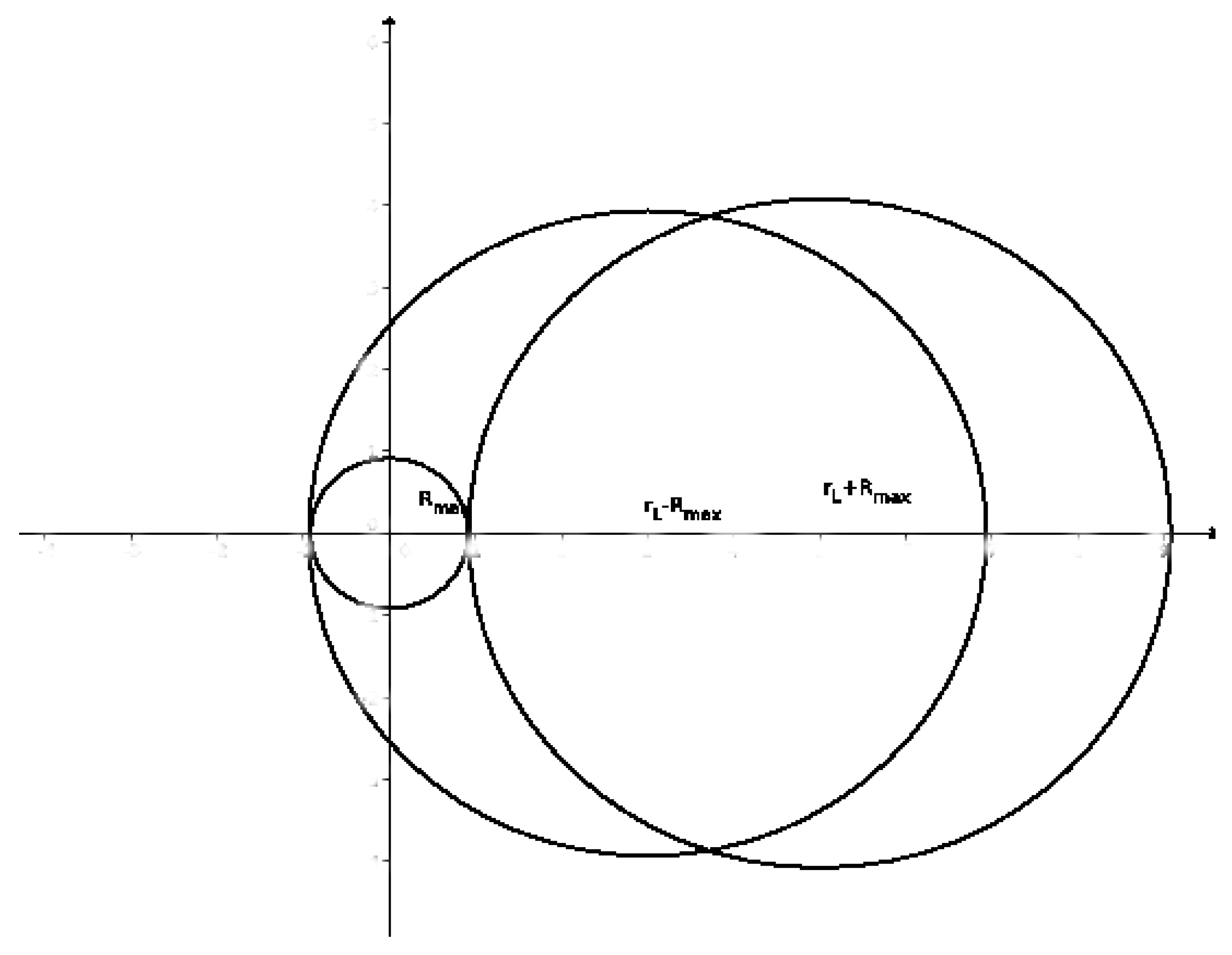
For , as depicted in Figure 2: is necessary for the x-y component of the trajectory to be no larger than .
This means
Hence for and for .
Hence a spiraling perturber at a distance from the z-axis, still “just" becomes relevant when it comes closest to the z-axis in its spiraling trajectory. Note that since the Larmor radius depends on the perpendicular velocity component, the cylinder-radius depends on the perpendicular velocity.
Hence the impact parameter is in
i.e., the impact parameter lies in a disk or annulus depending on whether is larger or smaller than .
2.3. Cylinder Length
From Equation (4) we obtain for and :
Hence the length of the cylinder for a given , and is determined by accounting for all particles in the above interval, i.e., the length is
2.4. Collision Volume
The collision-time statistics method first computes the number of relevant particles, i.e., the density times the relevant volume, i.e., the above cylinder. This volume is:
with and denoting a one and two-dimensional Maxwellian velocity distributions respectively. and are:
and
As already mentioned, the number of particles that are in this volume, and hence need to be simulated, is simply the volume multiplied by the perturber density. The computation of the collision volume V is detailed in Appendix A. Although with the above Collision-time statistics modification, all relevant particles are accounted for, some that are accounted for may actually not contribute. Hence the simplified version described here is still inefficient for very small magnetic field (or large mass) and does not recover the B = 0 (i.e., Seidel [4,5]) result. For instance, it does not account for the fact that for very small B (or large mass), is very small and very large, so that a particle initially at does not have the time to reach the interaction region. However, in this work we stick to this approach because it is efficient for electrons and magnetic fields that are not too small and is much simpler. For ions this approach may well be inadequate, as the dimensionless factor q defined in the appendix, which is essentially the ratio of is often and the Collision-time statistics method as described here results in a large number of ions that must be accounted for, due to the larger , even though not all of them are effective. For example, for conditions relevant to white dwarfs, e.g., electron density e/cm, T = 5 eV and , for ions (protons) and 26 for electrons for . Among other things, this means that ions are far from completing a single spiral, while electrons complete several. As a result, an ion that starts at a distance in the x-y plane close to will fail to enter the interaction region (sphere with radius ) in (0,) and hence need not be accounted for at all. The present method is too generous with such perturbers and hence is inadequate for ions. Its extension is left for future work. Note, however, that this discussion applies to the efficiency of the calculation, not the results.
2.5. Generating Perturbers
To generate perturbers, we first draw a random number uniformly distributed in (0,1). If this is smaller than , then we generate from the distribution by generating independently a with the probability distribution , a with the probability distribution and a with the probability density in .
Otherwise we generate from the distribution . The generation of impact parameters was done by a rejection method, as straightforward inversion is not possible.
Once and have been generated, is selected as a uniformly distributed time in .
Last, an angle , uniformly distributed in () is generated, so that and .
2.6. The Line Profile
Then the Schrödinger equation is solved for the atomic system in the field generated by the thus-drawn plasma particle and the resulting time evolution (U-matrices) are used to obtain the autocorrelation function
with denoting upper level states and lower level states for the line in question. This is repeated for a large number of such field histories in order to obtain reliable statistics and at the end a Fourier transform is taken to obtain the line profile.
3. Calculations Results
For the calculations we only considered the hydrogen line. Although at the parameters discussed in [1] ions may be dominant, only electrons were considered in the present work, in order to make contact with similar work [1] (which is also why a simplified version was used as discussed above).
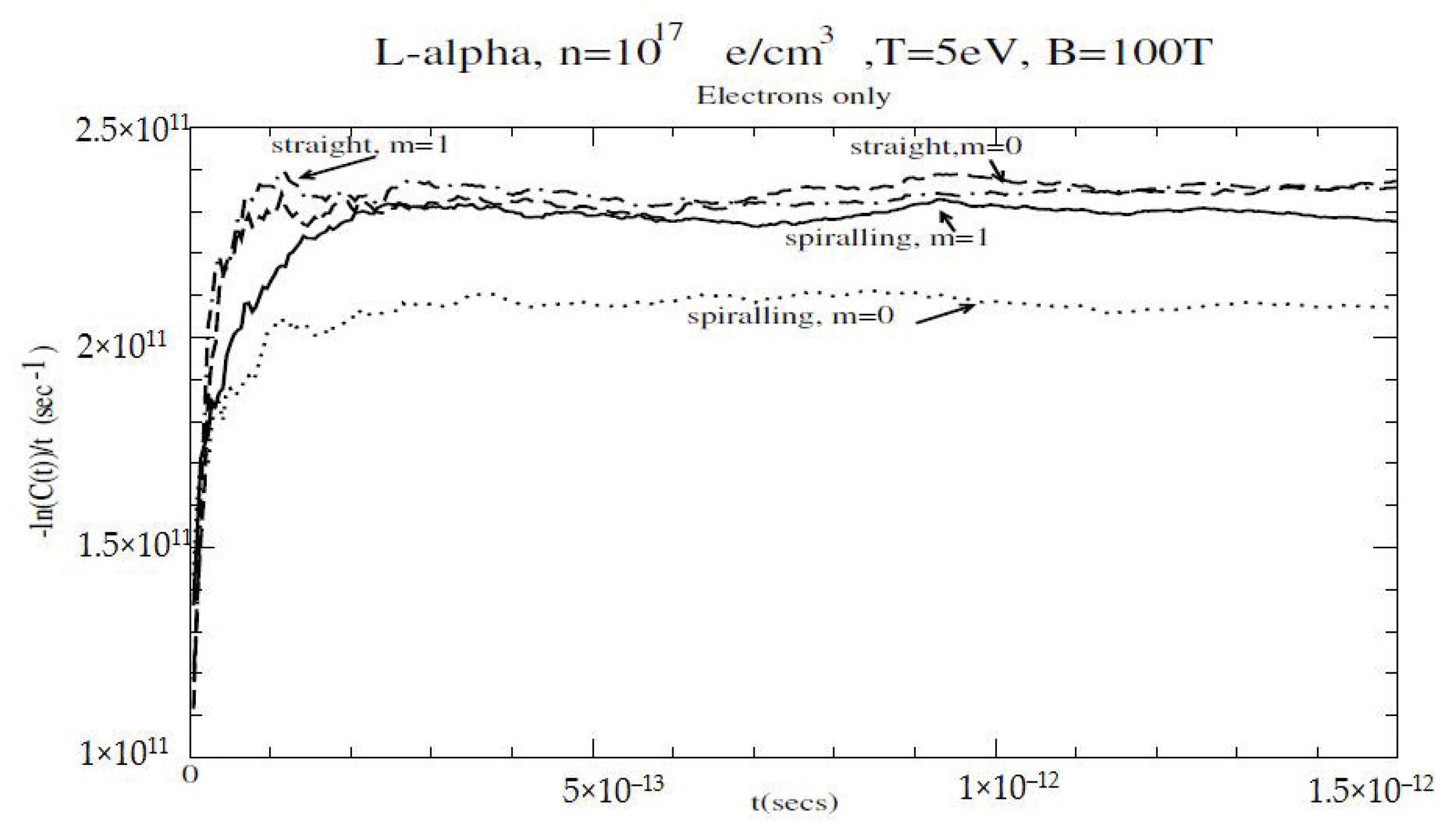
was used as in Table 1. Note that the autocorrelation function , i.e., the Fourier transform of the lineshape has not dropped to negligible levels even for ; however, for all cases extrapolation was employed, as an impact form was detected for , as depicted in Figure 3. In that case C(t) has dropped to about 70% of its t = 0 value for .
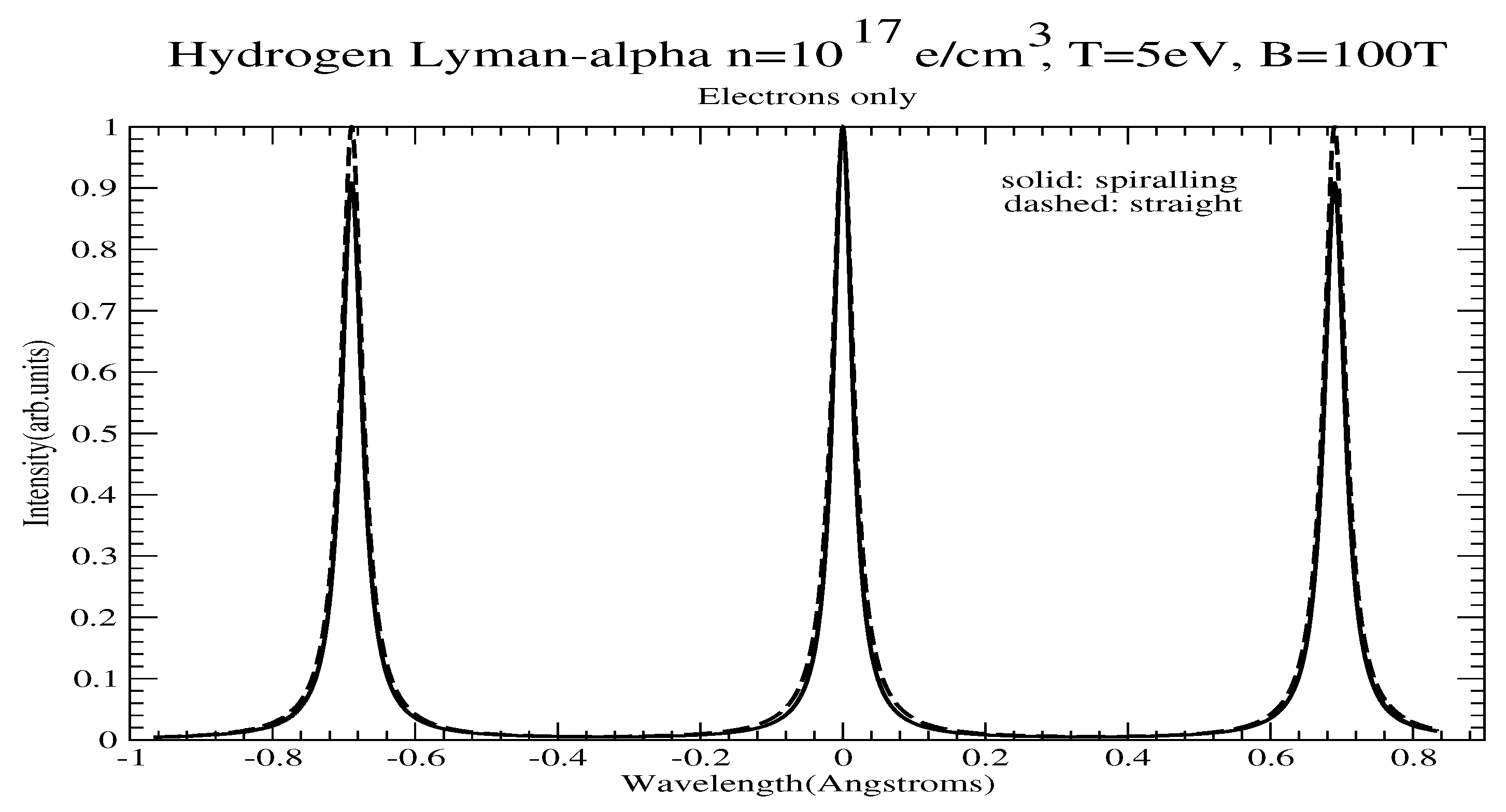
Also shown are the final profiles in Figure 4 for both parallel (unshifted) and perpendicular directions to the field.
4. Physical Discussion
The present work differs from the work in Reference [1] in that (a) it is not limited to cases where the shielding length exceeds the Larmor radius, (b) it includes the contribution of particles with impact parameters larger than the shielding length, (c) it is non-perturbative and (d) accounts for overlapping collisions, although for (c) and (d) a corresponding impact calculation could be done along these lines, as the impact approximation is built-in the collision-time statistics technique. Note that Debye-shielded fields are used in the calculations in this work.
Compared to the situation without magnetic field, i.e., straight line trajectories, we note the following:
- More perturbers may participate in the broadening due to the larger cylinder width, e.g., in the x-y plane, impact parameters in () contribute, while they did not in the case of straight line trajectories. However, this is a contribution and offset by the fact that impact parameters in ( ) have a reduced contribution because such perturbers spend time outside . So if , this is not expected to have a significant effect. However, if , then only a small arc of the spiral may contribute to broadening, in the sense of providing for an appreciable interaction. This could be more interesting and is not considered in [1].
- On the other hand, the cylinder length can be shorter, as only the velocity component contributes and the one-dimensional average velocity is smaller than the three-dimensional one, hence the contribution may be smaller for the than for the case. The relative importance of compared to depends not only on the magnetic field and plasma parameters, but also on the “time of interest”, . As discussed, this is generally a few inverse HWHMs, but can be substantially smaller if an exponential form in the autocorrelation function is realized before then.
To illustrate, we consider the hydrogen line under conditions found in tokamaks and white dwarfs and display the number of perturbers N required and contributions of and as a function of electron density n, Temperature(T), magnetic field (B), and model. q is the ratio . SI units are used throughout.
Note that for the lowest density, dominates and electrons are effective than for the case, as discussed above. Since other things (shielding, distribution functions etc) are equal, this means smaller widths.
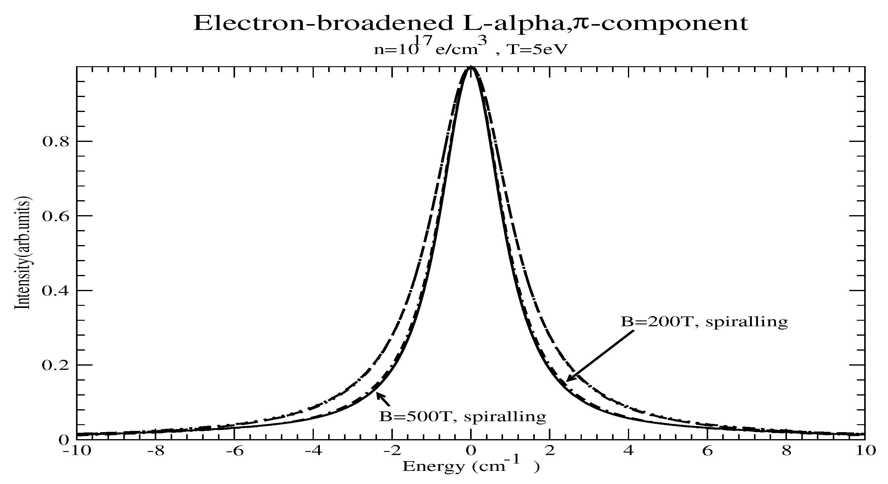
Figure 5 shows the -component of electron-broadened with (a) no magnetic field (dotted), (b) B = 200 T but no spiralling (dashed), (c) B = 500 T but no spiralling (dash-double dotted), (d) B = 200 T and spiralling (dot-double dashed) and (e) B = 500 T and spiralling (solid). Note that spiralling results in a line narrowing, and makes much more difference than a change in B, as the B = 0, 200 and 500 T results with no spiralling practically coincide.
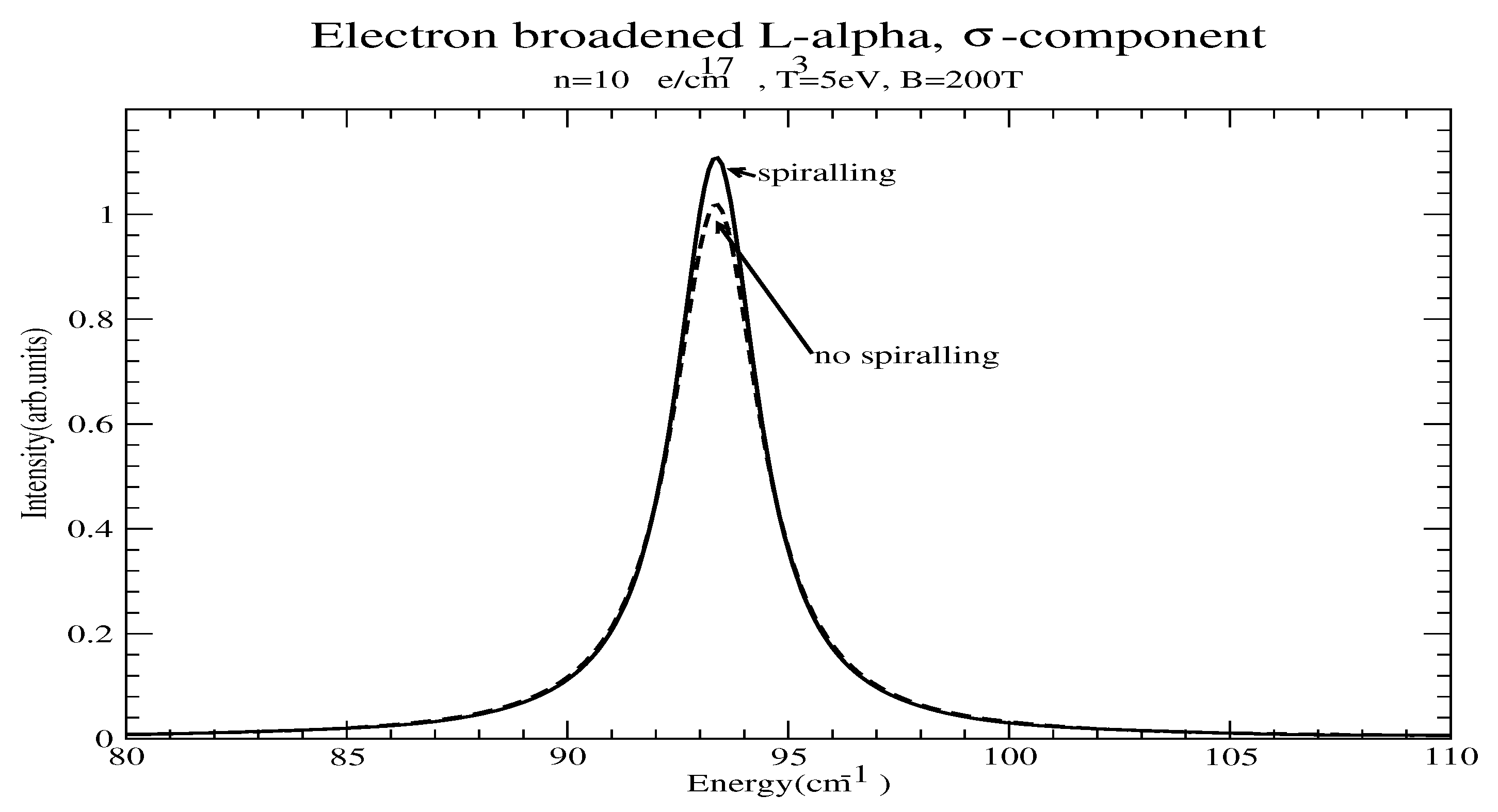
Similarly, Figure 6 shows the -component of electron-broadened for B = 200 T with no spiralling (dashed) and spiralling (solid), appropriately scaled. Again, spiralling results in a line narrowing.
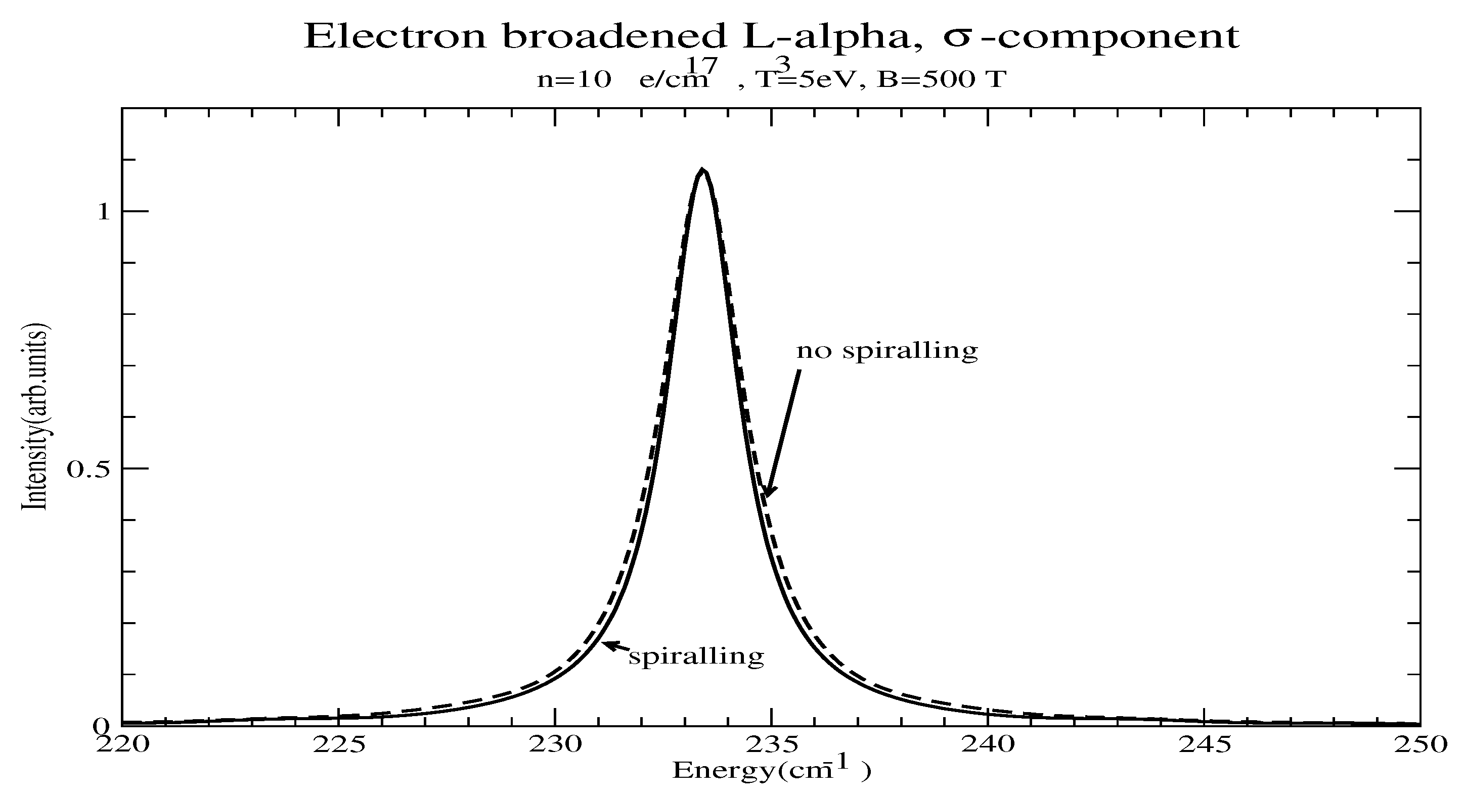
The same qualitative effect of narrowing due to spiralling is seen in Figure 7, which shows the -component of electron-broadened for B = 500 T with no spiralling (dashed) and spiralling (solid), appropriately scaled.
5. Shifts
In [1] shifts and further structure (e.g., triplet) of the component are also discussed as being associated with the spiralling trajectories and it is proposed that these are more characteristic features than broadening effects. In the approach of Reference [1], these shifts are a consequence of the removal of degeneracy of the upper level states because of the Zeeman effect and would be present regardless of the perturber motion, though the shift magnitude does, of course, depend on the exact form of the perturber-emitter interaction. In other words, the approach of the present work handles both widths and shifts with no conceptual difference: Due to Zeeman splitting, the emitter-plasma (interaction-picture) interaction V(t) acquires an imaginary exponential that slows down the decay of the autocorrelation function. This is too small to be observable in the examples shown. In any case, shifts are outside the scope of the present work.
Funding
This research received no external funding.
Conflicts of Interest
The author declares no conflict of interest.
Appendix A. Collision Volume Calculation
Starting with Equation (10), the integration in returns the average z-velocity , while it simply returns 1 for as does not appear at all.
with and T and m the perturber temperature and mass respectively,
and
Consequently
with (essentially the ratio ), denoting the upper incomplete Gamma function
and the average perpendicular velocity: . Note that
Consequently can be expressed as:
with the complementary error function. For note that ; however, as already discussed for q = 0 (B = 0) we still get a divergence.
While for
with
where we used .
The upper integration limit results in a square root of zero argument and hence only contributes
The lower integration limit, if 0 (i.e., ) contributes
while if the contribution is:
Hence
The velocity integration thus reads:
Substituting we have
where
and
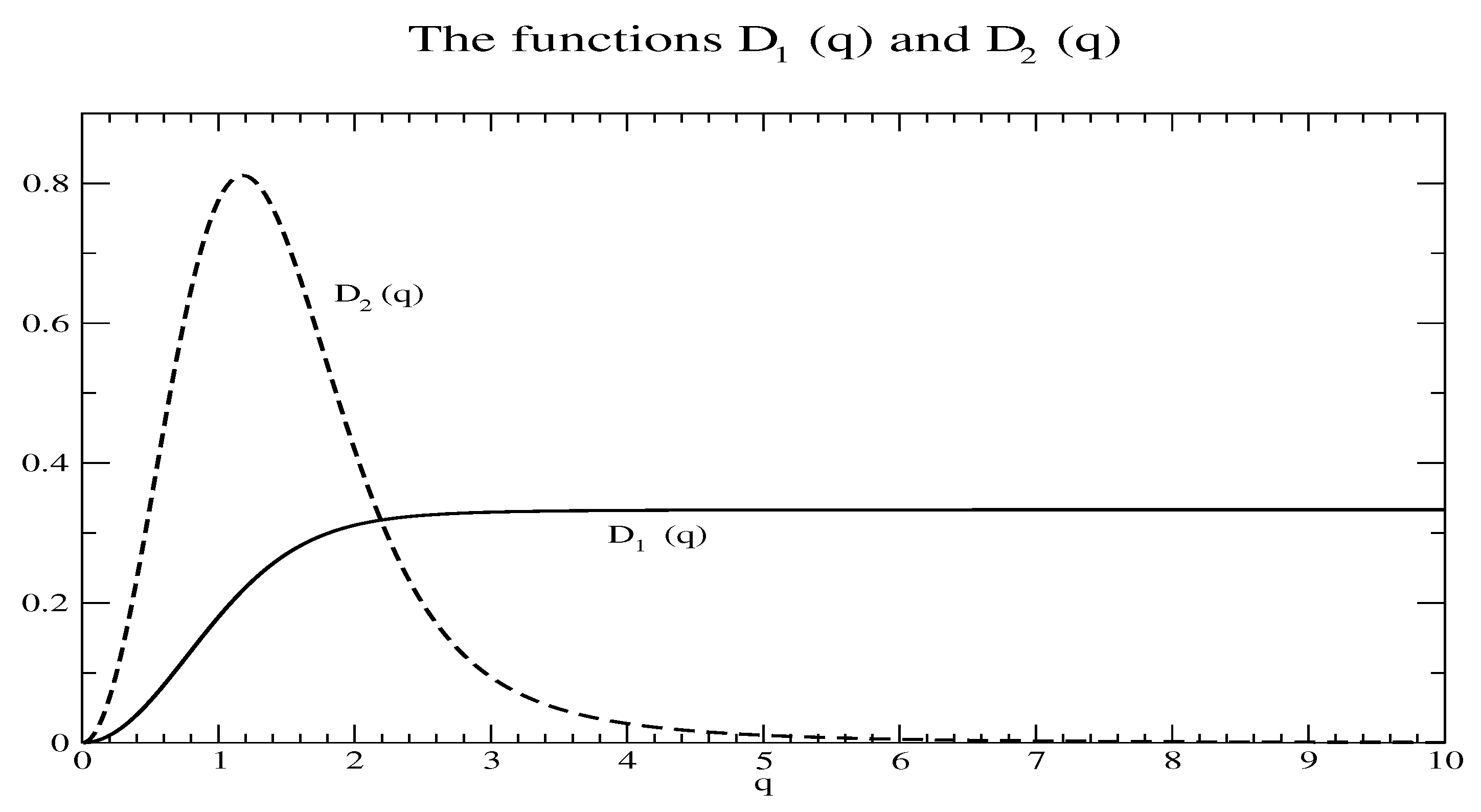
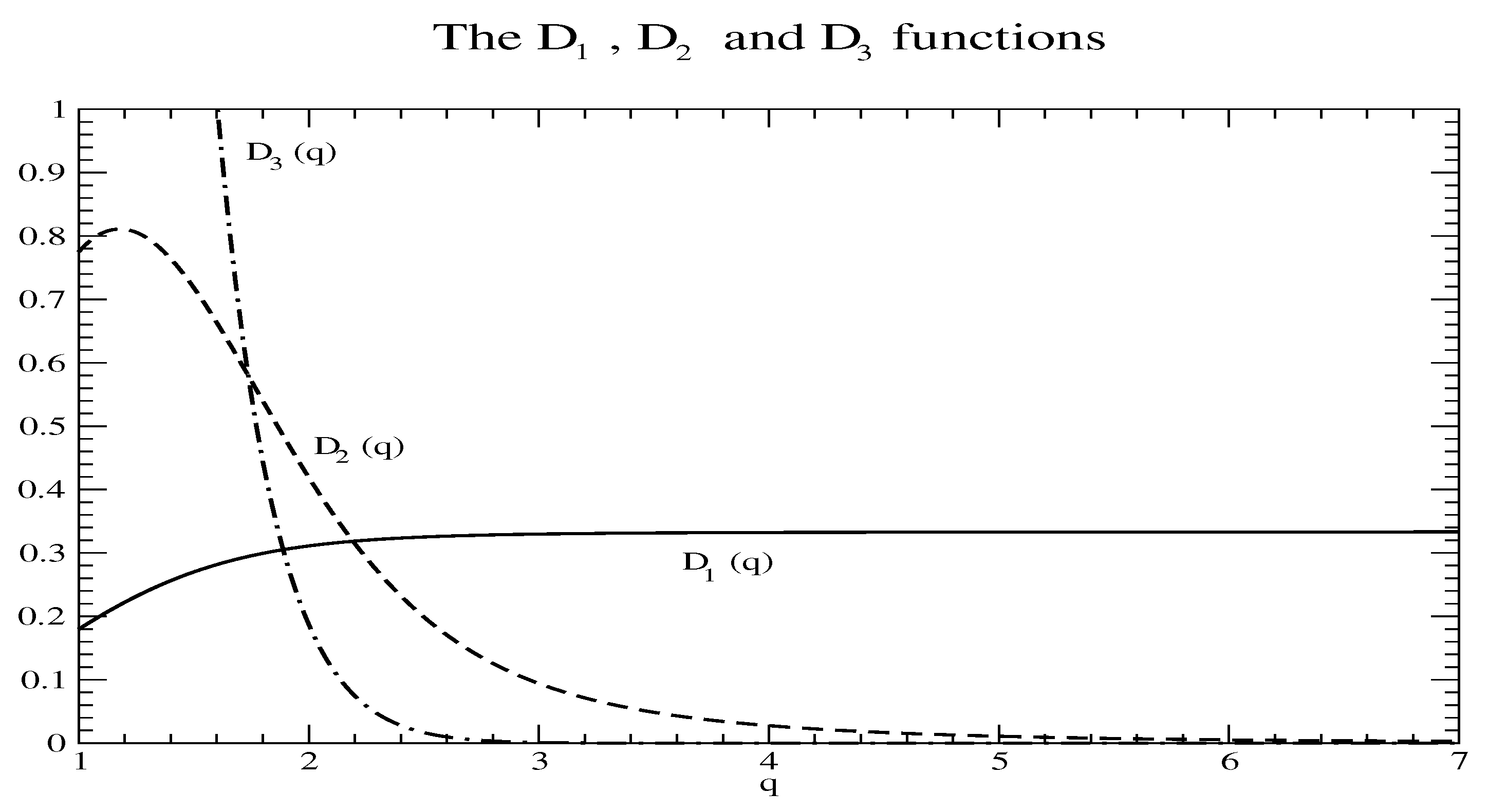
Note that because of the issue with small B mentioned, diverges as ; however, it quickly becomes negligible compared to and . The functions and are shown in Figure A1, while all three functions are shown for in Figure A2.
Hence
Figure A1.
The and functions.

Figure A2.
The , and functions for .

References
- Oks, E. Influence of magnetic-field-caused modifications of trajectories of plasma electrons on spectral line shapes: Applications to magnetic fusion and white dwarfs. J. Quant. Spectrosc. Radiat. Transf. 2016, 171, 15–27. [Google Scholar] [CrossRef]
- Deutsch, C. Electric microfield distributions in plasmas in presence of a magnetic field. Phys. Lett. A 1969, 30, 381–382. [Google Scholar] [CrossRef]
- Hegerfeld, C.G.; Kesting, V. Collision-time simulation technique for pressure-broadened spectral lines with applications to Ly − α. Phys. Rev. A 1988, 37, 1488–1496. [Google Scholar] [CrossRef]
- Seidel, J.; Verhandl, D.P.G. Spectral Line Shapes 6 (AIP Conference Proceedings); Frommhold, L., Keto, J.W., Eds.; New York, NY, USA, 1990; Volume 216. [Google Scholar]
- Alexiou, S. Implementation of the Frequency Separation Technique in general lineshape codes. High Energy Density Phys. 2013, 9, 375–384. [Google Scholar] [CrossRef]
- Rosato, J.; Ferri, S.; Stamm, R. Influence of helical trajectories of perturbers on Stark line shapes in magnetized plasmas. Atoms 2018, 6, 12. [Google Scholar] [CrossRef]
| 1. | In fact Reference [1] only deals with . |
Figure 1.
x-y trajectory projections for . The rightmost circle corresponds to a perturber with , so that the perturber is more than away from the emitter.
Figure 1.
x-y trajectory projections for . The rightmost circle corresponds to a perturber with , so that the perturber is more than away from the emitter.

Figure 2.
x-y trajectory projections for .

Figure 3.
Plot of the quantity , which is seen to saturate for large t, indicating that an impact form has set in. The conditions were e/cm, T = 5 eV and B = 100 T. 10,000 configurations were used in this run. m refers to the magnetic quantum number of the spherical states, i.e., the and () components of the autocorrelation function , as the lower level is not broadened.

Figure 4.
Line profile of the transitions with and without account of spiralling for e/cm, T = 5 eV and B = 100 T. 10,000 configurations were used in this run.
Figure 4.
Line profile of the transitions with and without account of spiralling for e/cm, T = 5 eV and B = 100 T. 10,000 configurations were used in this run.

Figure 5.
Line profile of the -compoment with and without account of spiralling for e/cm, T = 5 eV and B = 0, 200 and 500 T. The horizontal scale represents energy difference from the unperturbed line center.
Figure 5.
Line profile of the -compoment with and without account of spiralling for e/cm, T = 5 eV and B = 0, 200 and 500 T. The horizontal scale represents energy difference from the unperturbed line center.

Figure 6.
Line profile of the -compoment with and without account of spiralling for e/cm, T = 5 eV and B = 200 T. The horizontal scale represents energy difference from the unperturbed line center.
Figure 6.
Line profile of the -compoment with and without account of spiralling for e/cm, T = 5 eV and B = 200 T. The horizontal scale represents energy difference from the unperturbed line center.

Figure 7.
Line profile of the -compoment with and without account of spiralling for e/cm, T = 5 eV and B = 500 T. The horizontal scale represents energy difference from the unperturbed line center.
Figure 7.
Line profile of the -compoment with and without account of spiralling for e/cm, T = 5 eV and B = 500 T. The horizontal scale represents energy difference from the unperturbed line center.


Table 1.
Typical Number of perturbers required.
| n(e/cm) | T(eV) | B(Tesla) | Model | q | N | |||
|---|---|---|---|---|---|---|---|---|
| 12 | 0 | 150 | Electrons | 6,952,705 | 174 | |||
| 12 | 3 | 150 | Electrons | 4.44 | 4,955,646 | 126 | ||
| 5 | 0 | 150 | Electrons | 19,181 | ||||
| 5 | 100 | 150 | Electrons | 2.09 | 20,216 | |||
| 5 | 0 | 180 | Ions | 2222 | ||||
| 5 | 100 | 180 | Ions | 0.069 | 1,364,429,438 |
© 2019 by the author. Licensee MDPI, Basel, Switzerland. This article is an open access article distributed under the terms and conditions of the Creative Commons Attribution (CC BY) license (http://creativecommons.org/licenses/by/4.0/).
Share and Cite
MDPI and ACS Style
Alexiou, S. Line Shapes in a Magnetic Field: Trajectory Modifications I: Electrons. Atoms 2019, 7, 52. https://doi.org/10.3390/atoms7020052
AMA Style
Alexiou S. Line Shapes in a Magnetic Field: Trajectory Modifications I: Electrons. Atoms. 2019; 7(2):52. https://doi.org/10.3390/atoms7020052
Chicago/Turabian StyleAlexiou, Spiros. 2019. "Line Shapes in a Magnetic Field: Trajectory Modifications I: Electrons" Atoms 7, no. 2: 52. https://doi.org/10.3390/atoms7020052
Note that from the first issue of 2016, this journal uses article numbers instead of page numbers. See further details here.