Analytical Solution of the Hanle Effect in View of CLASP and Future Polarimetric Solar Studies

Abstract

We have solved a problem of the Hanle effect for the hydrogen Lyman-$\alpha$ line in an intuitive and straightforward way. The Stokes parameters amid an anisotropic radiation field and a magnetic field are derived as an analytical formula which enables us to conduct immediate analyses of observation data taken by spectro-polarimetry. The derived formula is, in particular, supposed to be used for the analysis of the data taken by CLASP (Chromospheric Lyman-Alpha Spectro-Polarimeter), which has aimed at measuring the linear polarization in the hydrogen Lyman-$\alpha$ line (121.6 nm) and then evaluating the magnetic field in the upper chromosphere and the transition region. The dependence of the Stokes parameters on the strength and direction of the magnetic field and on the observation angle is derived with our analytical model. The results show a satisfactory agreement with those of a more rigorous numerical calculation where the radiative transfer is taken into account and the consistency is assured between the anisotropic randiation field and the polarized atomic state.

1. Introduction

Problems in solar physics such as coronal heating and flare triggering are still open and they all are thought to be caused by the magnetic field. Information on the magnetic field helps us perform mode identification or evaluation of the energy flux of Magnetohydrodynamic waves [1]. Moreover, a change of the magnetic field vector after a flare gives us information on where the reconnection has taken place and how much magnetic field energy has been released. Measurement of the magnetic field is therefore important for solving many problems in solar physics. A number of measurements have been attempted to date. Indeed, the Spectro-Polarimeter (SP) of the Solar Optical Telescope (SOT) onboard the Hinode satellite has revealed the detailed magnetic field structures on the photosphere using the Zeeman effect [2]. On the other hand, very few measurements have been made of the magnetic field in the upper chromosphere and in the transition region, which is believed to be more critical for the corona problem because energy propagation and dissipation are large, thus reconnection frequently takes place. Because the magnetic field in those layers is so weak that the Zeeman splitting of spectral lines is veiled by the large Doppler broadening, using the same technique as SOT/SP is difficult.

Instead, the Hanle effect has been proposed as another possibility for the measurement of the magnetic field in those layers. Atoms in the solar atmosphere are excited by an anisotropic radiation field, which gives rise to unequal population distribution over the magnetic sublevels, the so-called atomic polarization, and the subsequent radiation is polarized. If there exists a magnetic field at the same time, the polarization is generally relaxed to some extent by the Hanle effect.

Actually, ground-based observations of the Hanle effect have been performed so far for the chromospheric lines in the visible and infrared ranges such as He I triplet at 1083 nm and Ca I at 422 nm [3], and the validity of the methodology has been confirmed. Other candidates for exploring the magnetic field in the high atmospheric layers are the strong resonance lines in the UV range [4,5,6] allowing us to access even the transition region. A representative line among them is the hydrogen Lyman-$\alpha$ ($1\mathrm{s}{}^2\mathrm{S}$–$2\mathrm{p}{}^2\mathrm{P}$, 121.6 nm).

Nevertheless, no measurement has been made for the Lyman-$\alpha$ line because the earth’s atmosphere is opaque to this line and thus a measurement in space is necessary. Recently, the CLASP (Chromospheric Lyman-Alpha Spectro-Polarimeter) project has carried out a high-precision spectro-polarimetric observation by a sounding rocket for the first time [7] and succeeded in detecting significant polarization signals in the Lyman-$\alpha$ line [8]. Great efforts are now being made to understand the detected polarization signals [9,10,11] and to determine the magnetic field vectors in the chromosphere and transition region from them.

In such circumstances, we have attempted to derive an analytical formula for calculating the observable Stokes parameters of the hydrogen Lyman-$\alpha$ for a given set of the magnetic field vector, the anisotropic radiation field, and the line-of-sight (LOS) of the observation. Trujillo Bueno et al. [5] have already developed a more thorough numerical code for the same purpose, which takes into account the consistency in the polarization states of the radiation field and of the atomic level. To be more precise, the problems of the radiative transfer and the population distribution over magnetic sublevels in the atoms are solved iteratively. However, complete understanding of the observation data has yet to be obtained to date, and an extended model, which, for example, is influenced by small perturbations in the magnetic field, is considered to be necessary. The analytical formula presented here would be useful for such extended calculations because it is easy to incorporate into other numerical codes. In addition to that, the analytical formula allows us to easily calculate the expected polarization signals, which are useful to investigate the influence of atmospheric model on the Hanle diagnostics [12] and other advantageous spectral lines.

Casini et al. [13] have also derived analytical formula of the Stokes parameters for describing the Hanle effect in the formalism of the irreducible spherical tensor representation [14]. We instead adopt the standard representation for developing the formula where emphasis is placed on having an intuitive understanding of the phenomenon. It is also noted that the present study assumes two important conditions. The first assumption is that the radiation field has an axis symmetry with respect to the direction normal to the solar surface. The CLASP observation has suggested that horizontal inhomogeneities of the solar chromosphere play an important role for production of linear polarization of the Lyman-$\alpha$ line [10,12]. Therefore, an application of the results derived here for actual observation data would require further fine customization. Secondly, optically thin conditions in the core of the Lyman-$\alpha$ line are assumed throughout the analysis although the atmosphere is known to be generally optically thick for the Lyman-$\alpha$. However, the radiation anisotropy is created only in the region having the unit optical depth [5], and the polarized light which we observe, though it could be only a small fraction, should originate in the optically thin part in the line formation.

2. Hanle Effect

2.1. Anisotropic Irradiation and Atomic Polarization

We assume instant photo-excitation and subsequent radiative decay, the time scale of which is governed by the spontaneous transition probability. When the excitation occurs successively, this model can also describe a steady-state condition when the time scale of change of the background plasma parameters is long enough. Recent Lyman-$\alpha$ imaging observations with the ultimate temporal cadence of 0.6 sec by CLASP discovered ubiquitous fast-propagating disturbances along the bright elongated structures with the time scale of a few tens of seconds [15], while the time scale of the Lyman-$\alpha$ line radiation is approximately 1.5 ns.

A two-level atomic system is considered. The lower level is the ground state $1\mathrm{s}{}^2\mathrm{S}$ and the upper state is $2\mathrm{p}{}^2\mathrm{P}$. The atoms in the ground state are excited to the upper state predominantly by the photo-absorption process. The radiation field is assumed to be axisymmetric with respect to the direction normal to the solar surface. Here, the quantization axis is first taken in the direction of the axis of symmetry of the radiation field.

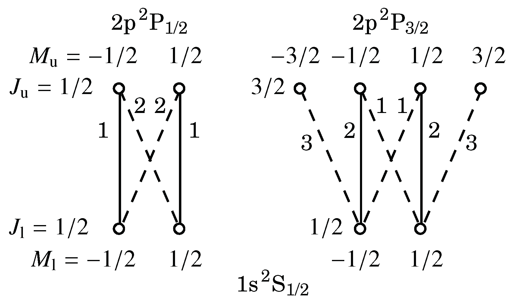
The excited state $2\mathrm{p}{}^2\mathrm{P}$ consists of two fine structure levels, i.e., $2\mathrm{p}{}^2{\mathrm{P}}_{3/2}$ and $2\mathrm{p}{}^2{\mathrm{P}}_{1/2}$. Figure 1 shows the Kastler diagram for the levels under consideration.

The solid and dashed lines correspond to the $\Delta M=0$ and $\Delta M=\pm 1$ transitions, respectively, where $\Delta M$ is the change of the magnetic quantum number M between the initial and the final states. The spontaneous transition probabilities between lower and upper magnetic sublevels are proportional to the square of corresponding transition matrix elements which can be calculated from the reduced matrix element for the transition between J-states including all pairs of magnetic sublevels with the help of the Wigner–Eckart theorem [16]. In Figure 1, the number next to each line indicates the relative transition probabilities. When the transitions considered are those between magnetic sublevels, i.e., both the upper and lower states are not degenerate, the relative absorption coefficients are the same as those for the spontaneous transition probabilities.

It is here assumed that the incident light to the atom is an equally mixed state of the right- and left-handed circularly polarized lights and that the ground level is unpolarized. Since the $J=1/2$–$1/2$ line, where J is the total angular quantum number, is never polarized under this condition, only the $J=3/2$ level is considered as the upper state when Stokes parameters Q and U components are calculated. In the actual observation, the Doppler width is so large that it is difficult to measure these two fine structure lines separately. Specifically, the temperature at the Lyman-$\alpha$ line center is approximately ${10}^4$ K [17], which corresponds to $7\times {10}^{-3}$ nm in the full width at half maximum, while the wavelength difference between the two fine structure lines is $5\times {10}^{-4}$ nm. Therefore, the $J=1/2$–$1/2$ line intensity is taken into account when the Stokes parameter I or the total intensity is considered.

The quantum condition of the excited state, i.e., the population distribution over the magnetic sublevels and the coherence among the sublevels, is expressed by the density matrix [14]. The density matrix of the upper level $\rho$ in the $|JM\rangle$ basis right after an instant excitation can be written as

$$\begin{array}{cc}\hfill \rho & =\left(\begin{array}{cccc}{\rho }_{\frac{3}{2}\frac{3}{2}}& {\rho }_{\frac{3}{2}\frac{1}{2}}& {\rho }_{\frac{3}{2}-\frac{1}{2}}& {\rho }_{\frac{3}{2}-\frac{3}{2}}\\ {\rho }_{\frac{1}{2}\frac{3}{2}}& {\rho }_{\frac{1}{2}\frac{1}{2}}& {\rho }_{\frac{1}{2}-\frac{1}{2}}& {\rho }_{\frac{1}{2}-\frac{3}{2}}\\ {\rho }_{-\frac{1}{2}\frac{3}{2}}& {\rho }_{-\frac{1}{2}\frac{1}{2}}& {\rho }_{-\frac{1}{2}-\frac{1}{2}}& {\rho }_{-\frac{1}{2}-\frac{3}{2}}\\ {\rho }_{-\frac{3}{2}\frac{3}{2}}& {\rho }_{-\frac{3}{2}\frac{1}{2}}& {\rho }_{-\frac{3}{2}-\frac{1}{2}}& {\rho }_{-\frac{3}{2}-\frac{3}{2}}\end{array}\right)=\left(\begin{array}{cccc}{\rho }_{\frac{3}{2}}& 0& 0& 0\\ 0& {\rho }_{\frac{1}{2}}& 0& 0\\ 0& 0& {\rho }_{\frac{1}{2}}& 0\\ 0& 0& 0& {\rho }_{\frac{3}{2}}\end{array}\right),\hfill \end{array}$$

(1)

where ${\rho }_{M^{\prime }{M}^{″}}$ represents the matrix element $\langle M^{\prime }|\rho |M^{″}\rangle$. The diagonal elements ${\rho }_{\frac{1}{2}}$ and ${\rho }_{\frac{3}{2}}$ are determined by the degree of anisotropy of the radiation field. The symmetry of $\rho$ with respect to the sign of M, i.e., ${\rho }_{\frac{3}{2}\frac{3}{2}}={\rho }_{-\frac{3}{2}-\frac{3}{2}}\equiv {\rho }_{\frac{3}{2}}$ and ${\rho }_{\frac{1}{2}\frac{1}{2}}={\rho }_{-\frac{1}{2}-\frac{1}{2}}\equiv {\rho }_{\frac{1}{2}}$, is ascribed to the fact that the incident light to the atom is an equally mixed state of the right- and left-handed circularly polarized lights so that there is no orientation. The density matrix is assumed to be normalized such that its trace is equal to unity, i.e.,

$$\begin{array}{c}\hfill 2{\rho }_{\frac{3}{2}}+2{\rho }_{\frac{1}{2}}=1.\end{array}$$

(2)

The population distribution over the magnetic sublevels is determined by the excitation rates under the present assumption. When the incident light propagates in the direction perpendicular to the quantization axis and is linearly polarized such that the electric field in the light oscillates parallel to the quantization axis, which is called the $\pi$-light, only the $\Delta M=0$ transitions occur. In that case, the density matrix elements of the excited state are expressed by ${\rho }_{\frac{1}{2}}=1/2$ and ${\rho }_{\frac{3}{2}}=0$. When the incident light propagates parallel to the quantization axis, the light is regarded as an equally mixed state of the right- and left-handed circularly polarized lights, which are both called the $\sigma$-light, and only cause $\Delta M=\pm 1$ transitions. In this case, the condition of ${\rho }_{\frac{1}{2}}=1/8$ and ${\rho }_{\frac{3}{2}}=3/8$ is expected. When the radiation field is isotropic, i.e., the same intensity in the all $\pi$-light and right- and left-handed $\sigma$-light components, the density matrix is scalar, i.e., ${\rho }_{\frac{1}{2}}={\rho }_{\frac{3}{2}}=1/4$. In general cases, ${\rho }_{\frac{1}{2}}$ and ${\rho }_{\frac{3}{2}}$ are determined by the ratio of the $\pi$-light and $\sigma$-light intensities, which are here denoted by $I_0$ and $I_{\pm 1}$. Since the incident light to the atom is an equally mixed state of the right- and left-handed circularly polarized lights, $I_1=I_{-1}$ is always preserved in the following discussion.

The photo-excitation rate from $|J_{\mathrm{l}}{M}_{\mathrm{l}}\rangle$ state to $|J_{\mathrm{u}}{M}_{\mathrm{u}}\rangle$ state, which is here denoted as $T_{M_{\mathrm{l}}{M}_{\mathrm{u}}}$, is given as [18]

$$\begin{array}{cc}\hfill T_{M_{\mathrm{l}}{M}_{\mathrm{u}}}& =\frac{8{\pi }^3}{3{ϵ}_0{h}^{2}c}{n}_{J_{\mathrm{l}}{M}_{\mathrm{l}}}\sum _q{\left|\langle J_{\mathrm{u}}{M}_{\mathrm{u}}|d_{-q}|J_{\mathrm{l}}{M}_{\mathrm{l}}\rangle \right|}^2{I}_q({\nu }_{M_{\mathrm{l}}{M}_{\mathrm{u}}}),\hfill \end{array}$$

(3)

where ${ϵ}_0$, h, and c are the permittivity of vacuum, Planck constant, and the speed of light, respectively, $n_{J_{\mathrm{l}}{M}_{\mathrm{l}}}$ is the population of the lower state $|J_{\mathrm{l}}{M}_{\mathrm{l}}\rangle$, $d_{-q}$ are the spherical components of the electric dipole operator, and $I_q({\nu }_{M_{\mathrm{l}}{M}_{\mathrm{u}}})$ are the spherical components of the radiation field intensity at the transition frequency ${\nu }_{M_{\mathrm{l}}{M}_{\mathrm{u}}}$. The anisotropy of the Lyman-$\alpha$ radiation field or the inequality between $I_0$ and $I_{\pm 1}$ in the solar atmosphere can be evaluated with a model of the solar atmosphere. In the literature, the anisotropy is often expressed by the irreducible tensor components $J_Q^K$ [14]. The relationship between $I_q$ and $J_Q^K$ is given as [18]

$$\begin{array}{cc}\hfill I_q& =\sum _K{(-1)}^{1+q}\frac{\sqrt{2K+1}}{3}\left(\begin{array}{ccc}1& 1& K\\ q& -q& 0\end{array}\right)J{}_0^K.\hfill \end{array}$$

(4)

In the present case of axisymmetry, the summation in Equation (4) is dominated by the terms of $J_0^2$ and $J_0^0$ [18]. Finally, ${\rho }_{\frac{1}{2}}$ and ${\rho }_{\frac{3}{2}}$ are obtained as

$$\begin{array}{cc}\hfill {\rho }_{\frac{1}{2}}& =\frac{T_{\frac{1}{2}\frac{1}{2}}+T_{-\frac{1}{2}\frac{1}{2}}}{T_{\frac{1}{2}\frac{3}{2}}+T_{\frac{1}{2}\frac{1}{2}}+T_{\frac{1}{2}-\frac{1}{2}}+T_{-\frac{1}{2}\frac{1}{2}}+T_{-\frac{1}{2}-\frac{1}{2}}+T_{-\frac{1}{2}-\frac{3}{2}}}=\frac{1}{4}\left(1-\frac{1}{\sqrt{2}}\frac{J_0^2}{J_0^0}\right),\hfill \end{array}$$

(5)

$$\begin{array}{cc}\hfill {\rho }_{\frac{1}{2}}& =\frac{T_{\frac{1}{2}\frac{3}{2}}}{T_{\frac{1}{2}\frac{3}{2}}+T_{\frac{1}{2}\frac{1}{2}}+T_{\frac{1}{2}-\frac{1}{2}}+T_{-\frac{1}{2}\frac{1}{2}}+T_{-\frac{1}{2}-\frac{1}{2}}+T_{-\frac{1}{2}-\frac{3}{2}}}=\frac{1}{4}\left(1+\frac{1}{\sqrt{2}}\frac{J_0^2}{J_0^0}\right).\hfill \end{array}$$

(6)

The $J_0^2/J_0^0$ value for the Lyman-$\alpha$ line in the solar atmosphere is available in Trujillo Bueno et al. [5], for example.

2.2. Effect of Magnetic Field

The polarization state of the upper level is modified during the spontaneous decay when there is a magnetic field. The influence of the magnetic field is described by a time-dependent density matrix, where the magnetic field is treated as a perturber. It is convenient to turn the quantization axis into the direction of the magnetic field, which is accomplished by rotations of the coordinates.

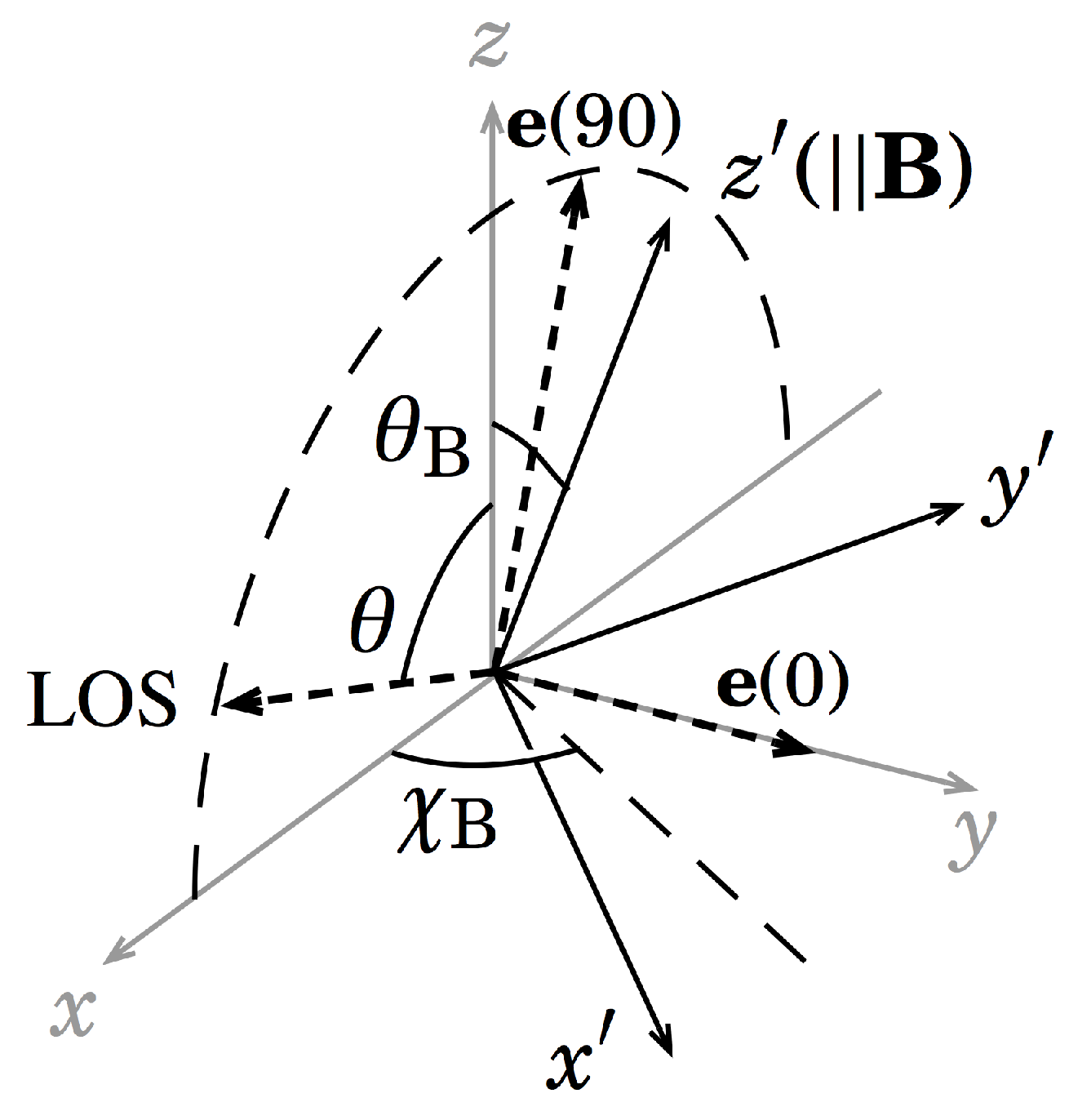
We define the coordinates to stipulate the geometrical relationship among the observation point on the solar surface, LOS, and magnetic field direction as follows and as depicted in Figure 2.

In the Cartesian coordinates, we take the origin at the observation point and z-axis in the direction normal to the solar surface. The x-axis is taken such that the LOS lies on the x–z plane, and the y-axis is chosen such that the three axes compose the right-handed-system. The inclination of the LOS from the z-axis is defined as $\theta$, the azimuth with respect to the z-axis of the magnetic field vector measured from the x-z plane in the counterclockwise direction observed from the positive z direction is defined as ${\chi }_{\mathrm{B}}$, and the inclination of the magnetic field from the z-axis is denoted as ${\theta }_{\mathrm{B}}$. When the change of the coordinates is conducted in accordance with the Euler’s rotation scheme, it is expressed with the two angles defined above, i.e., ${\chi }_{\mathrm{B}}$ and ${\theta }_{\mathrm{B}}$.

The density matrix elements in the new coordinates as a result of rotation R are expressed as

$$\begin{array}{cc}\hfill {\left({\rho }_{M{M}^{\prime }}\right)}_{\mathrm{B}}& =\sum _{m{m}^{\prime }}{\mathcal{D}}_{mM}^{(J)*}(R){\mathcal{D}}_{m^{\prime }{M}^{\prime }}^{(J)}(R)\langle m|\rho |m^{\prime }\rangle \hfill \end{array}$$

(7)

$$\begin{array}{c}=\sum _m{\mathcal{D}}_{mM}^{(J)*}(R){\mathcal{D}}_{m{M}^{\prime }}^{(J)}(R)\langle m|\rho |m\rangle ,\hfill \end{array}$$

(8)

where ${(\dots )}_{\mathrm{B}}$ indicates that the quantity inside the parentheses is described under the new coordinates and the last line is obtained because $\rho$ is diagonal in the present case. The rotation matrix elements ${\mathcal{D}}_{m{M}^{\prime }}^{(J)}(R)$ and ${{\mathcal{D}}_{mM}^{(J)}}^{*}(R)$ are each broken into two parts as

$$\begin{array}{cc}\hfill {\mathcal{D}}_{m{M}^{\prime }}^{(J)}(R)& =e^{-\mathrm{i}m{\chi }_{\mathrm{B}}}{d}_{mM}^{(J)}({\theta }_{\mathrm{B}}),\hfill \end{array}$$

(9)

$$\begin{array}{cc}\hfill {{\mathcal{D}}_{mM}^{(J)}}^{*}(R)& ={(-1)}^{m-M}{e}^{\mathrm{i}m{\chi }_{\mathrm{B}}}{d}_{-m-M}^{(J)}({\theta }_{\mathrm{B}}),\hfill \end{array}$$

(10)

where $d_{mM}^{(J)}({\theta }_{\mathrm{B}})$ is given by the Wigner’s formula [16]. The density matrix elements under the new coordinates are thus derived from those under the original coordinates. Hereafter, we develop the discussion with the new coordinates and the label ${(\dots )}_{\mathrm{B}}$ will be omitted from all the quantities.

We use the density matrix under this new coordinates and then consider its temporal development in the fixed magnetic field environment. The time-dependent density matrix is obtained as a solution of the equation of motion, which is written as

$$\begin{array}{cc}\hfill i\hslash \frac{\mathrm{d}}{\mathrm{d}t}\rho & =\left[H_{\mathrm{F}},\rho \right],\hfill \end{array}$$

(11)

where $\hslash =h/(2\pi )$. The matrix elements of the Hamiltonian due to the magnetic field perturber $H_{\mathrm{F}}$ are given as

$$\begin{array}{cc}\hfill \langle M|H_{\mathrm{F}}|M^{\prime }\rangle & ={\mu }_{B}gMB{\delta }_{M{M}^{\prime }}=\hslash {\omega }_{0}M{\delta }_{M{M}^{\prime }},\hfill \end{array}$$

(12)

where ${\mu }_B$ and g are the Bohr magneton and the Landé g-factor, respectively, and ${\omega }_0={\mu }_{B}gB/\hslash$ is called the Larmor angular frequency. Equation (11) is found to be a set of 16 independent equations and each equation is readily solved as

$$\begin{array}{cc}\hfill {\rho }_{M^{\prime }M}(t)& ={\rho }_{M^{\prime }M}(0)e^{\mathrm{i}(M^{\prime }-M){\omega }_{0}t}.\hfill \end{array}$$

(13)

2.3. Line Intensity and Stokes Parameters

The intensity of a linear polarization component of a transition between two magnetic sublevels, $I_{M_{\mathrm{u}}{M}_{\mathrm{l}}}(\mathbf{e})$, is given as

$$\begin{array}{c}\hfill I_{M_{\mathrm{u}}{M}_{\mathrm{l}}}(\mathbf{e})=C_{\mathrm{D}}{w}_{M_{\mathrm{u}}}{\left|\langle J_{\mathrm{u}}{M}_{\mathrm{u}}|\mathbf{e}·\mathbf{d}|J_{\mathrm{l}}{M}_{\mathrm{l}}\rangle \right|}^2,\end{array}$$

(14)

where $w_{M_{\mathrm{u}}}$ is the population of the level $M_{\mathrm{u}}$, $\mathbf{d}=-\sum e\mathbf{r}$, where e is the elementary charge, is the electric dipole operator, and $\mathbf{e}$ is the unit vector in the direction of the linear polarization component to be measured. For example, when one measures the linear polarization component which is parallel (perpendicular) to the limb, $\mathbf{e}$ should be like $\mathbf{e}(0)$ ($\mathbf{e}(90)$) in Figure 2. That is, the notation $\mathbf{e}(n)$ here stands for the vector $\mathbf{e}$ which is rotated in the counter-clockwise direction seen from the observer by the angle of n degrees from $\mathbf{e}(0)$ in Figure 2. The geometrical factor $C_{\mathrm{D}}$ is given as [19]

$$\begin{array}{cc}\hfill C_{\mathrm{D}}& =\frac{{\omega }_{J_{\mathrm{u}}{J}_{\mathrm{l}}}^4}{2\pi c^3{l}^2},\hfill \end{array}$$

(15)

where ${\omega }_{J_{\mathrm{u}}{J}_{\mathrm{l}}}$ is the angular frequency of the line and l is the distance of the observer from the atoms. The interaction between the electric dipole and the radiation, $\mathbf{e}·\mathbf{d}$, is expanded as

$$\begin{array}{c}\hfill \mathbf{e}·\mathbf{d}=\sum _{q=-1}^1{(-1)}^q{e}_{-q}{d}_q,\end{array}$$

(16)

where $e_q$ is given as [19]

$$\begin{array}{cc}\hfill e_0& =\gamma ,\hfill \end{array}$$

(17)

$$\begin{array}{cc}\hfill e_{\pm 1}& =\mp \frac{1}{\sqrt{2}}(\alpha \pm \mathrm{i}\beta ).\hfill \end{array}$$

(18)

Here, the parameters $\alpha$, $\beta$, and $\gamma$ are the x-, y-, and z-axis components of $\mathbf{e}$ in the Cartesian coordinates, respectively. It is noted that in the present case depicted in Figure 2 the parameters correspond to the $x^{\prime }$-, $y^{\prime }$-, and $z^{\prime }$-axis components, respectively.

The total line intensity of the $J=3/2$ to $J=1/2$ transition is then given as a summation of all the possible combinations of the upper and lower magnetic sublevels as

$$\begin{array}{cc}\hfill I(\mathbf{e})& =\sum _{M_{\mathrm{u}},M_{\mathrm{l}}}{I}_{M_{\mathrm{u}}{M}_{\mathrm{l}}}(\mathbf{e})\hfill \\ & =C_{\mathrm{D}}\sum _{M_{\mathrm{u}}^{\prime },M_{\mathrm{u}}^{″},M_{\mathrm{l}}}\langle J_{\mathrm{u}}{M}_{\mathrm{u}}^{\prime }|{\rho }_{\mathrm{u}}|J_{\mathrm{u}}{M}_{\mathrm{u}}^{″}\rangle \hfill \end{array}$$

(19)

$$\begin{array}{c}\times \langle J_{\mathrm{u}}{M}_{\mathrm{u}}^{″}|\mathbf{e}·\mathbf{d}|J_{\mathrm{l}}{M}_{\mathrm{l}}\rangle \langle J_{\mathrm{l}}{M}_{\mathrm{l}}{|(\mathbf{e}·\mathbf{d})}^{†}|J_{\mathrm{u}}{M}_{\mathrm{u}}^{\prime }\rangle .\hfill \end{array}$$

(20)

The matrix elements of the operator $\mathbf{e}·\mathbf{d}$ and ${(\mathbf{e}·\mathbf{d})}^{†}$ are expanded with Equation (16) as

$$\begin{array}{c}\langle J_{\mathrm{u}}{M}_{\mathrm{u}}^{″}|\mathbf{e}·\mathbf{d}|J_{\mathrm{l}}{M}_{\mathrm{l}}\rangle \hfill \end{array}$$

(21)

$$\begin{array}{c}=\left\{\sum _{q=-1}^1{(-1)}^q{e}_{-q}\left(\begin{array}{ccc}{J}_{\mathrm{u}}& 1& J_{\mathrm{l}}\\ -M_{\mathrm{u}}^{″}& q& M_{\mathrm{l}}\end{array}\right)\right\}\times {(-1)}^{J_{\mathrm{u}}-M_{\mathrm{u}}^{″}}\langle J_{\mathrm{u}}||d||J_{\mathrm{l}}\rangle ,\hfill \end{array}$$

(22)

and

$$\begin{array}{c}\langle J_{\mathrm{l}}{M}_{\mathrm{l}}{|(\mathbf{e}·\mathbf{d})}^{†}|J_{\mathrm{u}}{M}_{\mathrm{u}}^{\prime }\rangle =\langle J_{\mathrm{u}}{M}_{\mathrm{u}}^{\prime }|\mathbf{e}·\mathbf{d}|J_{\mathrm{l}}{M}_{\mathrm{l}}{\rangle }^{*}\hfill \end{array}$$

(23)

$$\begin{array}{c}=\left\{\sum _{q=-1}^1{(-1)}^q{e}_{-q}^{*}\left(\begin{array}{ccc}{J}_{\mathrm{u}}& 1& J_{\mathrm{l}}\\ -M_{\mathrm{u}}^{\prime }& q& M_{\mathrm{l}}\end{array}\right)\right\}\times {(-1)}^{J_{\mathrm{u}}-M_{\mathrm{u}}^{\prime }}\langle J_{\mathrm{u}}||d||J_{\mathrm{l}}{\rangle }^{*},\hfill \end{array}$$

(24)

where the Wigner–Eckart theorem [16] is used. Equation (20) is then rewritten as

$$\begin{array}{cc}\hfill I(\mathbf{e})& =C_{\mathrm{D}}\sum _{M_{\mathrm{u}}^{\prime }{M}_{\mathrm{u}}^{″}}{\rho }_{M_{\mathrm{u}}^{\prime }{M}_{\mathrm{u}}^{″}}(0)\left\{\eta cos\left[(M_{\mathrm{u}}^{\prime }-M_{\mathrm{u}}^{″}){\omega }_{0}t\right]-\xi sin\left[(M_{\mathrm{u}}^{\prime }-M_{\mathrm{u}}^{″}){\omega }_{0}t\right]\right\}\hfill \\ \times |\langle J_{\mathrm{u}}||d||J_{\mathrm{l}}{\rangle |}^2,\hfill \end{array}$$

(25)

where $\eta$ and $\xi$ are, respectively, the real and the imaginary parts of the term

$$\begin{array}{c}\hfill {(-1)}^{2J_{\mathrm{u}}-(M_{\mathrm{u}}+M_{\mathrm{u}}^{\prime })}\sum _{M_{\mathrm{l}}}\left\{\sum _{q=-1}^1{e}_q\left(\begin{array}{ccc}{J}_{\mathrm{u}}& 1& J_{\mathrm{l}}\\ -M_{\mathrm{u}}& q& M_{\mathrm{l}}\end{array}\right)\right\}\left\{\sum _{q^{\prime }=-1}^1{e}_{q^{\prime }}^{*}\left(\begin{array}{ccc}{J}_{\mathrm{u}}& 1& J_{\mathrm{l}}\\ -M_{\mathrm{u}}^{\prime }& q^{\prime }& M_{\mathrm{l}}\end{array}\right)\right\}.\end{array}$$

(26)

The upper state density decays due to the spontaneous transition in the actual situation. We can include this effect into Equation (25) by multiplying Equation (25) with $exp(-g_{0}t)$, where $g_0$ is the spontaneous transition probability. The line intensity we actually observe is the time-integral from $t=0$ to ∞, which is calculated as

$$\begin{array}{cc}\hfill \overline{I}(\mathbf{e})& ={\int }_0^{\infty }I(\mathbf{e})e^{-g_{0}t}\mathrm{d}t\hfill \end{array}$$

(27)

$$\begin{array}{c}=C_{\mathrm{D}}|\langle J_{\mathrm{u}}||d||J_{\mathrm{l}}{\rangle |}^2\sum _{M_{\mathrm{u}}^{\prime }{M}_{\mathrm{u}}^{″}}{\rho }_{M_{\mathrm{u}}^{\prime }{M}_{\mathrm{u}}^{″}}(0)\frac{\eta g_0-\xi (M_{\mathrm{u}}^{\prime }-M_{\mathrm{u}}^{″}){\omega }_0}{g_0^2+{\left[(M_{\mathrm{u}}^{\prime }-M_{\mathrm{u}}^{″}){\omega }_0\right]}^2}.\hfill \end{array}$$

(28)

Conventionally, in the solar observation, the Stokes parameter Q is tailored to be the difference between the linear polarization components parallel and perpendicular to the nearest limb and to be positive when the parallel component is larger. The Stokes parameter U is calculated similarly but with the components rotated 45 degrees in the counterclockwise direction seen from the observer. Consequently, Q and U normalized to I are derived as

$$\begin{array}{cc}\hfill Q/I& =\frac{\overline{I}(0)-\overline{I}(90)}{\overline{I}(0)+\overline{I}(90)},\hfill \end{array}$$

(29)

$$\begin{array}{cc}\hfill U/I& =\frac{\overline{I}(45)-\overline{I}(135)}{\overline{I}(45)+\overline{I}(135)},\hfill \end{array}$$

(30)

where $\overline{I}(0)$ stands for $\overline{I}(\mathbf{e}(0))$ and similarly for others.

3. Results and Discussion

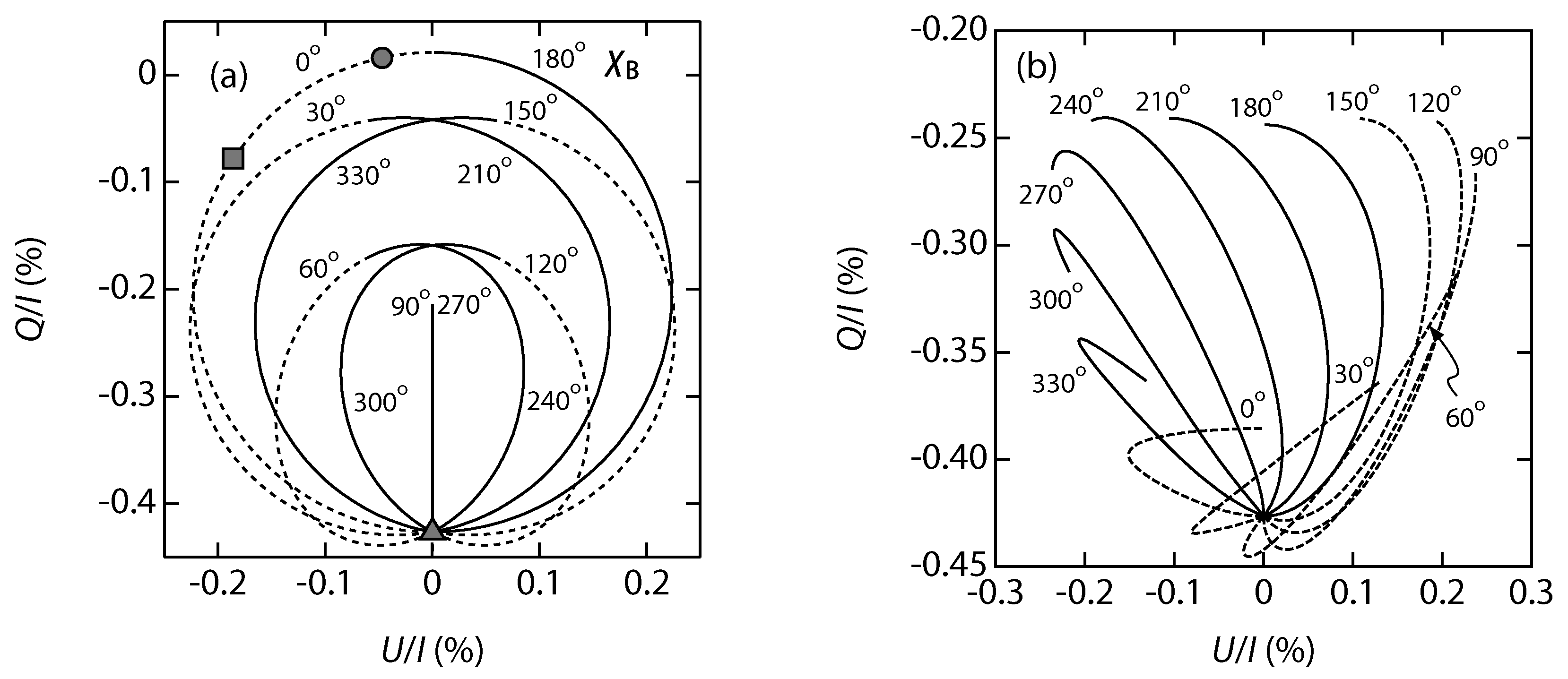
For examining the present results, we plot the Hanle diagrams with the Stokes parameters calculated with Equations (29) and (30) and compare them with Figure 3 and 4 in Ishikawa et al. [20], which are calculated based on Trujillo Bueno et al. [5]. It is noted that the values in Ishikawa et al. [20] are those at the line center whereas our result is the line intensity under the optically thin condition. The components in the $J=1/2$–$1/2$ transition which are unpolarized are taken into account for the Stokes I. The curves in Figure 3 show the B-dependence of the $Q/I$–$U/I$ relations for several different ${\chi }_{\mathrm{B}}$ values for a fixed $\mu =0.3$, where $\mu =cos\theta$, with (a) ${\theta }_{\mathrm{B}}={90}^{\circ }$ and (b) ${\theta }_{\mathrm{B}}={20}^{\circ }$.

The anisotropy of the radiation field $J_0^2/J_0^0$ for the initial density matrix is assumed to be $-0.01327$ so as to give the same $Q/I$ as Ishikawa et al. [20] under the condition of $\mu =0.3$ and $B=0$. This $J_0^2/J_0^0$ value is found to be consistent with the corresponding value in Figure 1 of Trujillo Bueno et al. [5]. It is readily noticed that the traces in both results closely overlap with each other, which confirms the validity of our method.

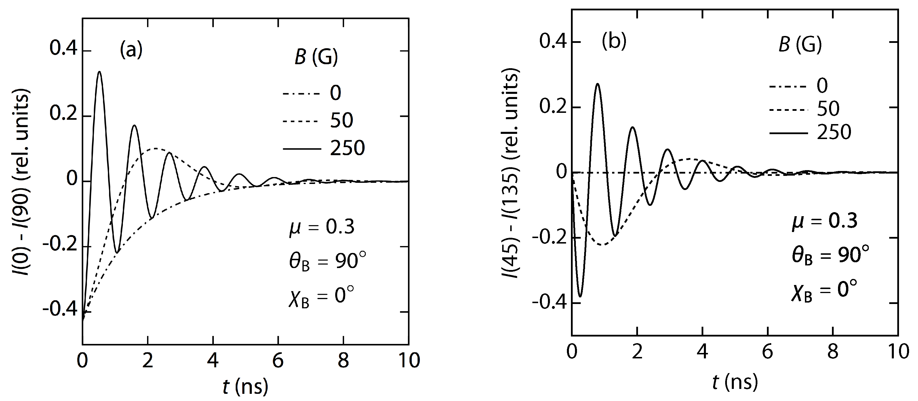
The results in Figure 3 are qualitatively understandable when the temporal development of the line intensity expressed by Equation (25) and the decay factor $exp(-g_{0}t)$ is taken into account. For example, the time-dependent quantities $I(0)-I(90)$ and $I(45)-I(135)$ which correspond to the Stokes parameter Q and U, respectively, are plotted in Figure 4 for several different B values with $\mu =0.3$, ${\theta }_{\mathrm{B}}={90}^{\circ }$, and ${\chi }_{\mathrm{B}}=0^{\circ }$.

When there is no magnetic field, $I(0)-I(90)$ is always negative as shown by the dash-dotted curve in Figure 4a and its integral over the entire time which corresponds to Q is negative. On the other hand, $I(45)-I(135)$ is fixed to be zero as shown by the dash-dotted curve in Figure 4b, which leads to $U=0$. These results are plotted by the triangle in Figure 3a.

At $B=50$ G, although $I(0)-I(90)$ takes positive values in the period between $t\sim 1$ ns and $t\sim 4$ ns as shown by the dashed curve in Figure 4a, Q is expected to be still negative. As for $I(45)-I(135)$, it starts to slowly oscillate with decreasing amplitude as shown by the dashed curve in Figure 4b. Since the dominant negative area in $t=0$ ns to $t\sim 2.5$ ns is larger than the positive area in $t\sim 2.5$ ns to $t\sim 5$ ns, it is understood that U takes a negative value. The square in Figure 3a shows these results.

When B is increased to 250 G, both the $I(0)-I(90)$ and $I(45)-I(135)$ show a rapid oscillation as shown by the solid curves in Figure 4a,b, respectively, and consequently, both Q and U should be close to zero as indicated by the circle in Figure 3a. At the limit of the strong magnetic field, it is inferred that the oscillation frequency of the curves becomes infinitely large and both Stokes parameters approach zero. It should be, however, noted that Q is found to converge to a small positive value instead of zero, as seen in Figure 3a.

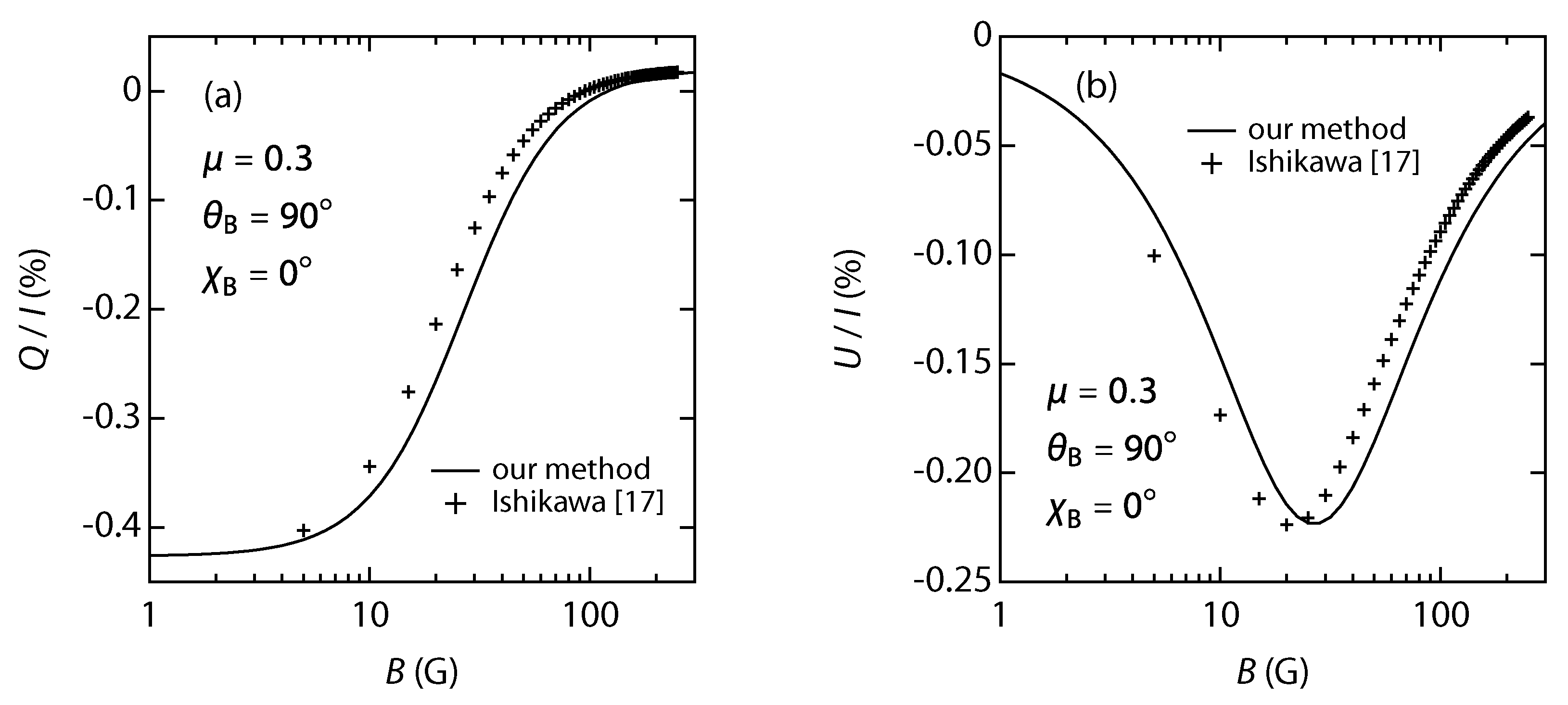
More detailed observation of the results, however, has revealed a slight difference in the B-dependence of the two calculations. Figure 5 shows (a) $Q/I$ and (b) $U/I$ as a function of B under the condition of $\mu =0.3$, ${\theta }_{\mathrm{B}}={90}^{\circ }$, and ${\chi }_{\mathrm{B}}=0^{\circ }$.

It is seen, for example, that the set of $Q/I$ and $U/I$ values at $B=25$ G with our calculation is obtained approximately at $B=20$ G with the result of Ishikawa et al. [20]. This could cause an overestimation of approximately 25% in the derived magnetic field strength when our method is used in the analysis.

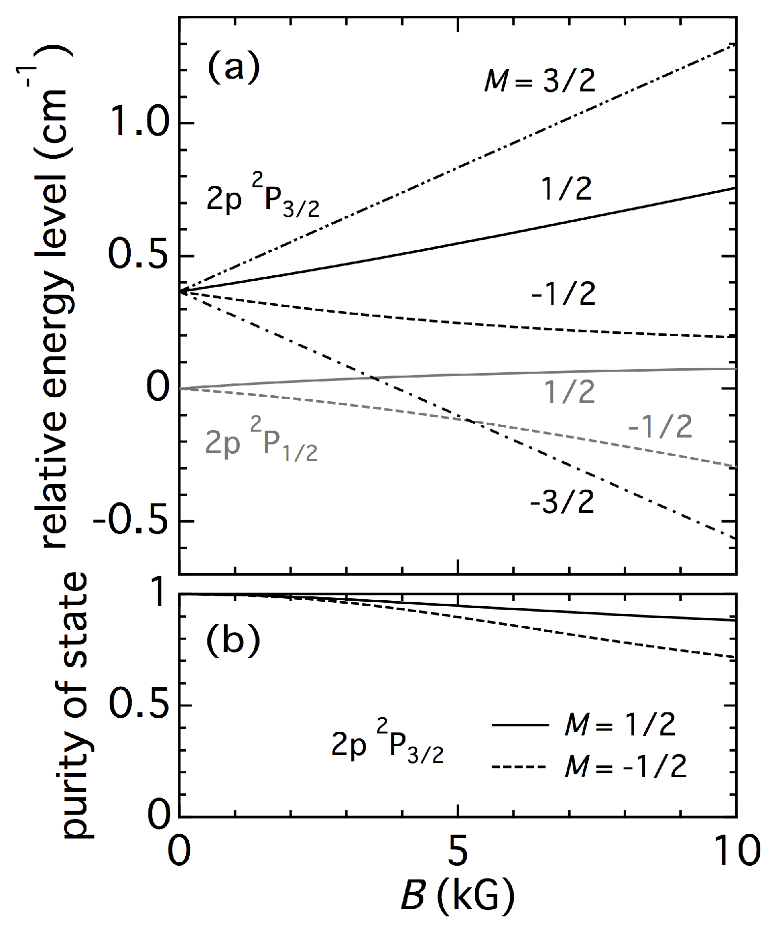
The reason for this difference could be ascribed to the omission of several effects in our method as compared with the complete numerical calculation. One difference between the two calculations is an omission of the quantum interference in our model. The quantum interference in the present case is the wavefunction mixing among the same M states in the $2\mathrm{p}{}^2{\mathrm{P}}_{3/2}$ and $2\mathrm{p}{}^2{\mathrm{P}}_{1/2}$ levels due to the magnetic field. Figure 6a shows the shifts of the magnetic sublevels in these two terms calculated by the method in Fujimoto and Iwamae [19].

The nonlinear behavior for the $M=1/2$ and $M=-1/2$ states is due to the wavefunction mixing. The solid black curve well represents the $2\mathrm{p}{}^2{\mathrm{P}}_{3/2,M=1/2}$ state under the weak magnetic field strength. As the field strength is increased J is no longer a good quantum number and the $2\mathrm{p}{}^2{\mathrm{P}}_{1/2,M=1/2}$ state partially mixes in. The solid black line in Figure 6b shows the composition fraction of the $2\mathrm{p}{}^2{\mathrm{P}}_{3/2,M=1/2}$ state in this mixed state or, in other words, the “purity” of the $2\mathrm{p}{}^2{\mathrm{P}}_{3/2,M=1/2}$ state. The dashed black line in the same figure shows a similar result for the $M=-1/2$ states. Although this effect is significant in the strong magnetic field case, its influence is confirmed to be negligible under the magnetic field weaker than 1 kG that is expected in the present study. Actually, the magnitude of the wavefunction mixing at 100 G is in the order of ${10}^{-4}$ and an influence in the same order of magnitude is expected on $Q/I$ and $U/I$. This amount of influence is insignificant in the final results like those in Figure 3.

Another important difference between the two calculations is that our method pays no attention to consistency between the polarization state of the ambient radiation field and of the radiation of atoms considered here. In the numerical calculation, the consistency is preserved by the iteration of the calculation until a convergence is obtained between the two radiation fields, where the radiative transfer equation plays a key role in deriving the polarization state of the radiation field from that of the local atomic radiation. This omission in our method could be a reason for the difference in the results of the two calculations.

Finally, a variety of uses are found for our analytical solution which facilitates incorporation of the Hanle effect into any simulation model. For example, Ishikawa et al. [12] has utilized this method for investigating the influence of the atmospheric model on the Hanle diagnostics. Another application can be considered when the magnetic field has a small perturbation term and the effect of the perturbation can be easily evaluated by linearization of the analytical formulas. We also emphasize that the application of our method is not limited to the hydrogen Lyman-$\alpha$ line but is also helpful for other resonance lines, such as Mg II k. Therefore, the present result should have a general significance for future solar research projects.

References

- Fujimura, D.; Tsuneta, S. Properties of magnetohydrodynamic waves in the solar photosphere obtained with Hinode. Astrophys. J. 2009, 702, 1443. [Google Scholar] [CrossRef]
- Tsuneta, S.; Ichimoto, K.; Katsukawa, Y.; Nagata, S.; Otsubo, M.; Shimizu, T.; Suematsu, Y.; Nakagiri, M.; Noguchi, M.; Tarbell, T.; et al. The Solar Optical Telescope for the Hinode Mission: An Overview. Sol. Phys. 2008, 249, 167–196. [Google Scholar] [CrossRef]
- Trujillo Bueno, J.; Merenda, L.; Centeno, R.; Collados, M.; Landi Degl’Innocenti, E. The Hanle and Zeeman Effects in Solar Spicules: A Novel Diagnostic Window on Chromospheric Magnetism. Astrophys. J. Lett. 2005, 619, L191–L194. [Google Scholar] [CrossRef] [Green Version]
- Belluzzi, L.; Trujillo Beuno, J. The polarization of the solar Mg II h and k lines. Astrophys. J. Lett. 2012, 750, L11. [Google Scholar] [CrossRef]
- Trujillo Bueno, J.; Štěpán, J.; Casini, R. The hanle effect of the hydrogen Lyα line for probing the magnetism of the solar transition region. Astrophys. J. Lett. 2011, 738, L11. [Google Scholar] [CrossRef]
- Trujillo Bueno, J.; Štěpán, J.; Belluzzi, L. The Lyα lines of H I and He II: A differential hanle effect for exploring the magnetism of the solar transition region. Astrophys. J. Lett. 2012, 746, L9. [Google Scholar] [CrossRef]
- Giono, G.; Ishikawa, R.; Narukage, N.; Kano, R.; Katsukawa, Y.; Kubo, M.; Ishikawa, S.; Bando, T.; Hara, H.; Suematsu, Y.; et al. Polarization Calibration of the Chromospheric Lyman-Alpha SpectroPolarimeter for a 0.1% Polarization Sensitivity in the VUV Range. Part II: In-Flight. Sol. Phys. 2017, 292, 57. [Google Scholar] [CrossRef]
- Kano, R.; Bueno, J.T.; Winebarger, A.; Auchère, F.; Narukage, N.; Ishikawa, R.; Kobayashi, K.; Bando, T.; Katsukawa, Y.; Kubo, M.; et al. Discovery of Scattering Polarization in the Hydrogen Lyα Line of the Solar Disk Radiation. Astrophys. J. Lett. 2017, 839, L10. [Google Scholar] [CrossRef]
- Ishikawa, R.; Bueno, J.T.; Uitenbroek, H.; Kubo, M.; Tsuneta, S.; Goto, M.; Kano, R.; Narukage, N.; Bando, T.; Katsukawa, Y.; et al. Indication of the Hanle Effect by Comparing the Scattering Polarization Observed by CLASP in the Lyα and Si iii 120.65 nm Lines. Astrophys. J. 2017, 841, 31. [Google Scholar] [CrossRef]
- Trujillo Bueno, J.; Štěpán, J.; Belluzzi, L.; Ramos, A.A.; Sainz, R.M.; Alemán, T.D.; Casini, R.; Ishikawa, R.; Kano, R.; Winebarger, A.; et al. CLASP Constraints on the Magnetization and Geometrical Complexity of the Chromosphere-Corona Transition Region. Astrophys. J. Lett. 2018, 866, L15. [Google Scholar] [CrossRef]
- Štěpánn, J.; Trujillo Bueno, J.; Belluzzi, L.; The CLASP Team. A Statistical Inference Method for Interpreting the CLASP Observations. Astrophys. J. 2018, 865, 48. [Google Scholar] [CrossRef] [Green Version]
- Ishikawa, R.; Uitenbroek, H.; Goto, M.; Iida, Y.; Tsuneta, S. Influence of the Atmospheric Model on Hanle Diagnostics. Sol. Phys. 2018, 293, 74. [Google Scholar] [CrossRef]
- Casini, R. The Hanle Effect of the Two-Level Atom in the Weak-Field Approximation. Astrophys. J. 2002, 568, 1056. [Google Scholar] [CrossRef]
- Blum, K. Density Matrix Theory and Applications; Plenum: New York, NY, USA, 1981. [Google Scholar]
- Kubo, M.; Katsukawa, Y.; Suematsu, Y.; Kano, R.; Bando, T.; Narukage, N.; Ishikawa, R.; Hara, H.; Giono, G.; Tsuneta, S.; et al. Discovery of Ubiquitous Fast-Propagating Intensity Disturbances by the Chromospheric Lyman Alpha Spectropolarimeter (CLASP). Astrophys. J. 2016, 832, 141. [Google Scholar] [CrossRef]
- Sakurai, J.J. Modern Quantum Mechanics; Addison-Wesley: Redwood City, CA, USA, 1985. [Google Scholar]
- Vernazza, J.E.; Avrett, E.H.; Loeser, R. Structure of the solar chromosphere. III—Models of the EUV brightness components of the quiet-sun. Astrophys. J. Suppl. 1981, 45, 635–725. [Google Scholar] [CrossRef]
- Degl’Innocenti, E.L.; Landolfi, M. Polarization in Spectral Lines; Burton, W.B., Ed.; Kluwer Academic Publishers: Dordrecht, The Netherlands, 2004. [Google Scholar]
- Goto, M. Zeeman and Stark Effects. In Plasma Polarization Spectroscopy; Fujimoto, T., Iwamae, A., Eds.; Splinger: Berlin, Germany, 2008. [Google Scholar]
- Ishikawa, R.; Ramos, A.A.; Belluzzi, L.; Sainz, R.M.; Štěpán, J.; Bueno, J.T.; Goto, M.; Tsuneta, S. On the inversion of the scattering polarization and the hanle effect signals in the hydrogen Lyα line. Astrophys. J. 2014, 787, 159. [Google Scholar] [CrossRef]
Figure 1.
Kastler diagram for the Lyman- line. The solid and dashed lines correspond to the and transitions, respectively. The numbers next to the lines indicate the relative line intensities when the population in the upper state is equally distributed over all the magnetic sublevels.
Figure 2.
Geometrical relationship among the observation point, that is, the origin of the coordinates, the line-of-sight (LOS), and the magnetic field direction.
Figure 3.
Example of Hanle diagram for with (a) and (b) . The triangle, square, and circle in (a) indicate the points at G, G, and G, respectively.
Figure 4.
Temporal variation of (a) and (b) . Here, only the level is taken into account as the upper state of the transition.
Figure 5.
B-dependence of (a) and (b) under the condition of , and .
Figure 6.
(a) energy level shifts of the magnetic sublevels in the hydrogen and states due to the Zeeman effect and (b) purity of the state for the and levels in the state.
© 2019 by the authors. Licensee MDPI, Basel, Switzerland. This article is an open access article distributed under the terms and conditions of the Creative Commons Attribution (CC BY) license (http://creativecommons.org/licenses/by/4.0/).
Share and Cite
MDPI and ACS Style
Goto, M.; Ishikawa, R.; Iida, Y.; Tsuneta, S. Analytical Solution of the Hanle Effect in View of CLASP and Future Polarimetric Solar Studies. Atoms 2019, 7, 55. https://doi.org/10.3390/atoms7020055
AMA Style
Goto M, Ishikawa R, Iida Y, Tsuneta S. Analytical Solution of the Hanle Effect in View of CLASP and Future Polarimetric Solar Studies. Atoms. 2019; 7(2):55. https://doi.org/10.3390/atoms7020055
Chicago/Turabian StyleGoto, Motoshi, Ryohko Ishikawa, Yusuke Iida, and Saku Tsuneta. 2019. "Analytical Solution of the Hanle Effect in View of CLASP and Future Polarimetric Solar Studies" Atoms 7, no. 2: 55. https://doi.org/10.3390/atoms7020055
Note that from the first issue of 2016, this journal uses article numbers instead of page numbers. See further details here.