Visual Tilt Estimation for Planar-Motion Methods in Indoor Mobile Robots

Computer Engineering Group, Faculty of Technology, Bielefeld University, D-33594 Bielefeld, Germany
Robotics 2017, 6(4), 32; https://doi.org/10.3390/robotics6040032
Submission received: 22 September 2017
/
Revised: 27 October 2017
/
Accepted: 28 October 2017
/
Published: 31 October 2017
Abstract
:Visual methods have many applications in mobile robotics problems, such as localization, navigation, and mapping. Some methods require that the robot moves in a plane without tilting. This planar-motion assumption simplifies the problem, and can lead to improved results. However, tilting the robot violates this assumption, and may cause planar-motion methods to fail. Such a tilt should therefore be corrected. In this work, we estimate a robot’s tilt relative to a ground plane from individual panoramic images. This estimate is based on the vanishing point of vertical elements, which commonly occur in indoor environments. We test the quality of two methods on images from several environments: An image-space method exploits several approximations to detect the vanishing point in a panoramic fisheye image. The vector-consensus method uses a calibrated camera model to solve the tilt-estimation problem in 3D space. In addition, we measure the time required on desktop and embedded systems. We previously studied visual pose-estimation for a domestic robot, including the effect of tilts. We use these earlier results to establish meaningful standards for the estimation error and time. Overall, we find the methods to be accurate and fast enough for real-time use on embedded systems. However, the tilt-estimation error increases markedly in environments containing relatively few vertical edges.
1. Introduction
Visual methods operating on images from a robot’s onboard camera have many applications in mobile robotics. These include relative-pose estimation [1], visual odometry [2,3], place recognition [4], and simultaneous localization and mapping (SLAM) [5]. Some of these visual methods are based on a planar-motion assumption: under this assumption, the robot travels in a flat plane without pitching or rolling. As a result, the robot moves with only three instead of six degrees of freedom (DOF), as illustrated in Figure 1. This simplification is used, for example, in visual relative-pose estimation [6,7,8,9,10,11] or place recognition [12]. We previously compared visual relative-pose estimation methods in the context of a domestic cleaning robot [1]. We found that planar-motion methods [9,10] can be more accurate and faster than their nonplanar counterparts [13,14].
However, even in a benign indoor environment, uneven ground may cause the robot to pitch or roll. Tilting the robot in such a manner violates the planar-motion assumption. For our pose-estimation experiments, this introduced large errors in the results [1]. Here, even a small tilt of ≈2° eliminated the quality advantage of the planar-motion methods. Larger tilts then increased these errors beyond those of the nonplanar motions. Such a small angle can be caused even by a slight roughness of the movement surface (see Section 2.3). Booij et al. [11] encountered a similar effect while testing planar-motion pose-estimation methods. The authors suspected tilts from an accelerating robot as the cause.
To tackle this problem, we estimate the tilt angle and tilt direction (Figure 1) with which an image was captured. A planar-motion method can then use this information to correct for tilts in the input image. The tilt could be measured using an additional sensor, such as an inertial measurement unit (IMU). However, this increases the cost and complexity of the robot, more so because the sensor needs to be calibrated [15] and synchronized relative to the camera. Instead, we estimate the tilt parameters from a single panoramic camera image by following the algorithm outlined in Figure 3. This estimate is based on vertical elements, which are commonly found in indoor environments. These elements are orthogonal to the floor, and thus orthogonal to the robot’s movement plane. Some of the elements will appear as edges in the camera image. Locating the vanishing point of these edges lets us determine the robot’s tilt. We evaluate our results in the context of the visual pose-estimation methods compared in [1]: the tilt-estimation accuracy should allow the planar-motion methods to remain competitive with their nonplanar counterparts. Furthermore, tilt estimation should add only a small overhead to the time required for planar-motion pose estimation.
1.1. Related Works
Visually estimating a camera’s orientation relative to the world is a prominent research problem. As in our work, vanishing points are widely used, and offer several advantages [16]: because they lie at infinity, their position is not affected by camera translation. Furthermore, the vanishing points are determined from an image’s edge pixels. Thus, many non-edge pixels can be disregarded, which speeds up processing time.
A popular class of methods assumes a Manhattan world, as described by Coughlan and Yuille [17]: here, image edges are assumed to belong to world elements that are either parallel or orthogonal to each other. These three orthogonal sets of parallel elements serve as the axes of a world coordinate system. One example for such a world is an environment consisting only of parallel cuboids.
Košecká and Zhang [18] present one early work based on the Manhattan world. The authors group edge pixels from nonpanoramic images into distinct straight lines. They then determine the Manhattan-world vanishing points from these lines using expectation maximization [19]. Denis et al. [20] compare several early Manhattan-world orientation-estimation methods. This work also introduces additional methods based on straight lines in nonpanoramic images. Tardif [21] uses the J-Linkage algorithm [22] to identify distinct vanishing points from straight image edges. This method then selects those three vanishing points that best correspond to the Manhattan directions. All of these works require straight image edges. For this reason, they are not directly applicable to our fisheye images, which contain strong radial distortions.
Bazin et al. [16] search panoramic images for edges belonging to straight elements in the world [23]. They then perform a coarse-fine search over the space of possible camera orientations. For a Manhattan world, each hypothetical orientation predicts a distinct set of vanishing points. This method selects the orientation under which the highest number of images edges are consistent with these predicted vanishing points. Another work by Bazin et al. [16] follows the same Manhattan-world approach. As before, orientations are scored by comparing their predicted vanishing points to the image edges. To find the best orientation, a branch-and-bound algorithm [24] divides the orientation space into intervals. Those intervals that contain only inferior solutions are discarded using interval analysis. The orientation estimate is then narrowed down by subdividing the remaining intervals.
In the Manhattan world, there are six (three orthogonal, plus their antipodals) vanishing points: one vertical pair, and two additional orthogonal pairs that lie on the horizon. Schindler and Dellaert [25] generalize this to an Atlanta world. In contrast to the Manhattan case, this world may contain additional vanishing point pairs located on the horizon. The authors estimate these vanishing points for nonpanoramic images using expectation maximization [19]. Tretyak et al. [26] also use an Atlanta-like world. They propose a scene model that encompasses lines, their vanishing points, and the resulting horizon and zenith location. The model parameters are then jointly optimized based on the edge pixels in a nonpanoramic image. Thus, the detection of lines, vanishing points, and the horizon and zenith are performed in a single step. However, these two methods assume images without radial distortion; thus, they cannot directly be used for our panoramic fisheye images.
Antone and Teller [27] also estimate camera orientations using vanishing points, but do not assume a specific world. Vanishing-point candidates are found by a Hough transform (survey: [28]), and then refined through expectation maximization [19]. The authors then identify a set of global vanishing points that appear across an entire collection of images. Camera orientations relative to these global vanishing points are then jointly estimated for all images. Lee and Yoon [29] also do not require a Manhattan or Atlanta world. Using an extended Kalman filter, they jointly estimate the vanishing points and camera orientations over a sequence. These two methods place no prior restrictions on the locations of vanishing points. Consequently, the alignment between the vanishing points and the robot’s movement plane is not known. To use them for tilt correction, this alignment must first be determined. Thus, these methods are not directly suitable to estimate the tilt from a single image.
The works discussed above estimate camera orientations relative to global vanishing points. Many other works determine the relative camera poses between two images [2,3]: one popular approach works by matching local visual features, such as those from the Scale-Invariant Feature Transform (SIFT) [30], between two images. The relative pose can then estimated from epipolar geometry [14]. However, these relative poses provide no information about the ground plane. Subsequently, they cannot be used to estimate tilts for planar-motion methods.
Some of the methods discussed here may also solve the tilt-estimation problem. For example, Bazin et al. [16] determine the camera orientation relative to a Manhattan world from a single panoramic image. However, we seek a solution that is optimized specifically towards tilt-estimation for planar-motion methods: within this problem, we need only the tilt angle and direction, and can ignore the robot’s yaw. These angles can be estimated from vertical elements alone, without requiring a full Manhattan or Atlanta world. Additionally, the tilt angle is bound to be small, which allows further simplifications. By exploiting these properties, we can can achieve good and fast tilt estimates using considerably simpler methods.
1.2. Contributions of This Study
In this work, we use two different visual methods to determine a robot’s tilt relative to a ground plane. We evaluate and discuss these methods within the context of a domestic floor-cleaning robot. These robots are a popular application of mobile robotics, being extensively sold on the commercial market. Our research group also has a long-standing interest in this application [31,32,33]. Specifically, we have previously developed a prototype for an autonomous floor-cleaning robot, shown in Figure 2.
Our prototype uses a planar-motion visual pose-estimation method [10] for localization and mapping. This method accurately estimates the relative camera pose between two images using very few computational resources [1]. However, the robot may tilt when driving over uneven ground, such as carpets or door thresholds. This violates the planar-motion assumption, which degrades the pose-estimation quality [1]. In this work, we use these results as a guide for designing experiments (Section 2.3 and Section 2.4) or evaluating results (Section 4). We also use our robot prototype to record a plausible image database, as described in Section 2.3. However, the methods presented here are not limited to this specific scenario; they may be used with other robots or planar-motion methods.
Both methods in this work operate on panoramic fisheye images, as captured by the robot’s on-board camera (Figure 3). These images show the hemisphere above the robot, but exclude everything below the horizon. Thus, the camera cannot see the ground plane, relative to which the tilt should be measured. Instead, we use vertical elements in the environment, which are orthogonal to the movement plane. Examples include room corners, door- and window frames, as well as the edges of furniture such as shelves. Some of these parallel elements appear as visually distinct edges in the robot’s camera images.
We now estimate the tilt parameters from the vanishing point of these edges: first, we apply an edge filter to the camera image and extract pixels with a strong edge response. Second, we identify the set of edge pixels belonging to vertical elements in the world, while rejecting those from non-vertical elements. Here, we assume that the tilt angle is small and that vertical elements far outnumber the near-vertical ones. Third, we determine the tilt angle and direction from the remaining edge pixels. Step one is identical for both methods, but steps two and three differ. The image-space method uses several approximations to simplify vanishing-point detection in the fisheye images. We then apply a correction factor to reduce the tilt-estimation errors introduced by these approximations. Operating directly on the panoramic fisheye image, this method is fast and simple to implement. In contrast, the vector-consensus method solves the tilt-estimation problem in 3D world coordinates. This method makes fewer approximations, but requires a calibrated camera model. It is also more similar to the existing vanishing-point methods discussed in Section 1.1.
We test the two methods on images recorded by the on-board camera of our cleaning-robot prototype. The robot was positioned at 43 locations spread across six different environments. At each location, we recorded images for the untilted and six different tilted configurations. The tilts estimated from these images were then compared to the ground truth, giving a tilt estimation error. We also measure the execution time required for tilt correction on a desktop and embedded system.
The rest of this work is structured as follows: Section 2.1 and Section 2.2 describe the two methods used in this work. We introduce the image database in Section 2.3, and the experiments in Section 2.4. Section 3 contains the results of these experiments, which we discuss in Section 4. Finally, we summarize our results and give an outlook to possible future developments in Section 5.
2. Materials and Methods
Our specific goal is to estimate the robot’s tilt angle and tilt direction , as shown in Figure 1. is given relative to the robot’s heading, with = 0° and = 90° describing a forward and leftward tilt, respectively. is measured relative to the robot’s untilted pose on a planar surface, thus, for an untilted robot, we have = 0°. We choose our world coordinate system so that is the surface normal of the movement plane. If is the normal vector in the coordinate system of a tilted robot, we then find that
Here, is the rotation matrix for the tilt , and atan2 is the quadrant-aware arctangent function. We can therefore determine by first determining . Both methods perform this step using visually distinct environment elements that are parallel to .
2.1. Image-Space Method
This method is based on the apparent location of the vertical elements’ vanishing point. is the point in the camera image where the vertical elements would appear to meet, if they were extended to infinity. We estimate using several problem-specific approximations, which simplify and speed up the method. We then determine the tilt parameters using the location of .
2.1.1. Preliminary Calculations
We first determine the vanishing point for an untilted robot, which we call . For convenience, we find using an existing camera calibration based on [34]. However, this point could also be determined separately, without requiring a fully calibrated camera. The calibrated camera model provides a projection function P. P maps the camera-relative bearing vector to the image point . Multiplying with the extrinsic rotation matrix R gives the bearing vector in robot coordinates. By definition, the surface normal is for an untilted robot. is parallel to the environment’s vertical elements, and consequently shares their vanishing point. Transforming into camera coordinates and projecting it gives us
If the robot is tilted, the apparent vanishing point will be shifted from . We will determine the tilt parameters from this shift. Figure 4 illustrates and for an untilted example image.
Note that it is irrelevant whether or not the camera image actually shows the environment at or around . Thus, this method would still work for robots where this part of the field of view is obscured. For a robot with an upward-facing fisheye camera, lies close to the geometric center of the image. However, this may not apply for an upward-facing camera that captures panoramic images using a mirror. Here, the image center corresponds to a direction below instead of above the robot. In this case, we can simply use the antipodal vanishing point of the vertical elements. This vanishing point lies below the robot, and thus we calculate from instead. Subsequent steps in the method then use this antipodal vanishing point.
2.1.2. Edge Pixel Extraction
As a first step towards tilt estimation, we detect edges in the camera image. We apply the Scharr operator to compute the horizontal and vertical edge gradients and for each pixel. This edge detector is somewhat similar to the popular Sobel operator, but was optimized to be invariant to edge orientation [35,36]. Since vertical elements can appear at any orientation within the image, this is a highly desirable property. In this work, we use the implementation provided by the OpenCV library [37]. Figure 5 contains an example of the resulting edge gradients.
We ignore pixels below the camera’s horizon, since they mostly show the robot’s chassis. We also reject pixels with a bearing of more than 45° above the camera horizon. Such pixels mainly show the ceiling, which contains horizontal elements that may be mistaken for vertical ones. To speed up computations, we only apply the Scharr operator to a bounding box around the remaining pixels. Finally, we discard pixels with a low gradient intensity . Such pixels are of limited use to us, since camera noise may strongly disturb their edge gradients. Eliminating these pixels also speeds up subsequent processing steps.
We do not try to identify straight lines of edge pixels, instead considering each pixel individually. This simplifies and speeds up our method, and lets us extract information even from very short edges. In contrast, combining connected pixels into long edges (as in [23]) may reduce the number of incorrect edge pixels, and may make the edge-gradient estimate more accurate [20]. However, within the scope of this work, we do not evaluate the trade-off between using individual edge pixels or long edges.
2.1.3. Edge Pixel Processing
Next, we estimate the tilt from the edge pixels identified in Section 2.1.2. For a camera with linear projection, a linear element in the environment would appear as a straight edge in the image. We can derive the edge direction for each pixel from the gradient . Extending each edge pixel along its edge direction result in a vanishing point, similar to Figure 4.
However, here we assume that the robot’s camera fits the model proposed by Scaramuzza et al. [34]; this panoramic camera model is not linear. Due to radial distortion, straight environment elements commonly appear as curves in the camera image. One example is given by the horizontal elements in Figure 4. However, for this tilt-estimation problem, we can use two simplifying approximations: first, we assume that vertical elements appear as straight edges in the panoramic image. This is approximately true for small tilt angles, as for example in Figure 6. Second, since is small, we assume that a tilt appears as a shift in the image. The edges and their vanishing point thus appear to move by a uniform amount (Figure 7c). In reality, tilting changes the orientation of these edges in the image. Due to the radial distortions of our fisheye lens, the vertical elements may also appear as curves (Figure 7b). Under our approximations, we ignore these effects and determine only an approximated vanishing point (Figure 6) instead of the actual vanishing point . This greatly simplifies our method, but also introduces tilt-estimation errors. We therefore apply a correction factor after estimating the tilt from the shift between and .
Panoramic Projections of Vertical Elements
We use the camera model to justify our previous assumption that vertical elements are projected linearly. According to the projection P [34], a bearing vector and corresponding image point are related by
Here, and are camera parameters, while . While refers to the actual pixel coordinates in the image, is the corresponding point in an idealized sensor plane. This idealized sensor plane is orthogonal to the optical axis, which corresponds to the camera’s z-axis. Figure 8 illustrates this camera model.
The coefficients of the polynomial function
are also camera parameters determined during calibration; in our experiments, we use . We now consider a straight line in space that is parallel to the camera’s optical axis. In camera coordinates, such a line consists of all points , which satisfy
where is a point on the line and . The bearing vector from the projection center to is simply ; here, is the unknown distance factor. From Equation (3), we see that the sensor-plane projection of this line must fulfill
We now express this projection in polar coordinates
and, from Equation (7), find that
is constant. Since the orientation for the projection of is constant, the vertical element appears as a straight line in the sensor plane. Because Equation (4) is linear, this also corresponds to a line in the final image.
From Equation (8), we note that the sensor-plane projections of all lines intersect at the origin point for . At this origin point, we have , and thus the distance factor from Equation (7) must be (except for lines with ). We now wish to find the specific point along a line that is projected to the sensor-plane origin. At this origin , and we thus evaluate
We can assume that , since Equation (3) would otherwise give a malformed bearing of for the origin .
We have now shown that lines parallel to the optical axis are projected linearly. Furthermore, these projections all meet at the vanishing point as Z approaches infinity. As per Equation (4), this point corresponds to in image coordinates. However, even for an untilted robot, the optical axis is usually not perfectly parallel to the vertical elements. Here, we assume that this misalignment is small for an upward-facing panoramic camera (≈0.16° in our cleaning-robot prototype, as calculated from the extrinsic calibration matrix R). We therefore choose to ignore this effect.
Approximating Tilts through Image Shifts
Next, we determine how tilting the robot affects the vanishing point of the vertical elements. A tilt is a rotation around an axis parallel to the movement plane, with . We derive the rotation matrix for such a tilt from by Rodrigues’ formula [38], with
For a small tilt angle , we approximate using and , which gives us
As discussed above, we assume that the optical axis is parallel to the vertical elements for an untilted robot. Thus, these elements are parallel to in camera coordinates. After rotating the camera around by a small angle , this is . According to Equation (3), the sensor-plane projection of obeys
Here, is sensor-plane location of the vanishing point for the tilted camera.
Since is small, this vanishing point shifts only a small distance from its untilted location of . In that case, , and we can approximate Equation (5) as . This approximation is favorable because for cameras with fisheye lenses, or parabolic or hyperbolic mirrors [34]. A tilt around the axis therefore shifts the vanishing point in proportion to the tilt angle :
Here, is the vanishing-point location in the actual image. The direction of this shift depends , and thus on the tilt direction .
Next, we estimate the shift of from the edge pixels extracted in Section 2.1.2. For each edge pixel k, we know the position , as well as the horizontal and vertical edge gradients and . From this, we calculate the gradient direction angle
This two-part definition ensures that is the same for both light-dark and dark-light edges. We also calculate the edge offset
is the distance between and a line orthogonal to that passes through . Figure 9 illustrates this geometry for a single edge pixel. If we treat k as part of an infinite, straight edge, would be the distance between that edge and . A similar parameterization for edge pixels was previously suggested by Davies [39]. For edge pixels k from vertical elements, we expect for an untilted robot. If the robot is tilted, will change based on the tilt parameters .
Tilt Parameters from Vanishing Point Shifts
In Figure 9, a tilt has shifted the vanishing point’s location from the expected point . The new vanishing point at is specified by the angle and the distance l from . Here, is the image-space tilt direction, from which we will later calculate the tilt direction of the robot. Due to this shift, the blue line extended from no longer passes through . According to Figure 9, the edge offset between the blue line and is
Using the trigonometric theorem of addition, we can rewrite this as
Each edge pixel k from a vertical element provides us with one instance of Equation (19). For N such edge pixels, we then have a system with two unknowns and N linear equations. We can solve this overdetermined system for using a linear least squares approach. This lets us determine
Knowing and l gives us the position of the approximate vanishing point.
Using as a substitute for the true location in Equation (15), we get
Recall that, for an untilted robot, we assume the optical axis to be orthogonal to the movement plane. In this case, Equation (2) simplifies to , and from this we can show that using Equations (3), (4) and (7). With this result, we can write Equation (22) as
with the magnitude . We note that the two vectors in square brackets both have a length of 1, and can therefore write
For a conventional camera with square pixels, we can approximate and , resulting in
Note that the tilt axis is given in the camera reference frame. Since we assume that the camera is mounted facing upwards, the z-axis of the robot and the camera should be parallel. However, the -axes of the robot and the camera may be rotated relative to each other. This rotation is described by the extrinsic calibration matrix R (Section 2.1.1). To estimate the tilt direction in the robot reference frame, we first determine the robot tilt axis
From , we can finally calculate the tilt direction
Note that Equation (29) includes the term because the tilt direction is at a right angle to the tilt axis.
We have made a number of approximations during this derivation. Most noticeably, we assume that a tilt causes a shift in the camera image, disregarding the effects shown in Figure 7. During preliminary experiments, we found that this method exhibits systematic errors in the estimated tilt angle . As per Equation (26), should be proportional to the shift distance l with a coefficient of . Since this gives poor results in practice, we replace the camera parameter with a correction factor a, so that
a is the proportionality constant relating l and , which we estimate from a set of training images using
Here, is the shift distance l measured for the image with index i. 0° is the ground truth for in the ith image, determined according to Section 2.3. Thus, a equals the mean ratio between the shift and true tilt angle over a training set of m tilted images. Using this heuristic, we can improve the accuracy of our estimates while still benefiting from the numerous simplifications made above.
2.1.4. Rejecting Incorrect Pixels
So far, we have assumed that all edge pixels correspond to vertical elements. This is not the case in a real environment, as shown by the many non-vertical elements in Figure 5. We therefore have to reject incorrect edge pixels caused by these non-vertical elements. Edge pixels disturbed by image artifacts and camera noise should also be filtered out.
As a first step, we apply a prefilter that discards all pixels with a large edge offset : as before, we assume a small tilt angle . According to Equation (30), an upper bound for also limits l. From Equation (18), we see that , and thus a limit on l implies a limit . We therefore discard edge pixels k with large , as they are not consistent with . After this prefiltering, the remaining edge pixels form the set F. In this work, we chose , which corresponds to 10°; the precise value of depends on the choice of a in Equation (30). Figure 10 shows the result of this prefiltering step.
We now estimate the tilt parameters by fitting a cosine to the of the edge pixels in the prefiltered set F. This step is described in Section 2.1.3 and illustrated in Figure 11. Here, incorrect edge pixels may cause large errors, as demonstrated by Figure 12a. Such pixels can arise from non-vertical elements or noise, as seen in Figure 13. One solution uses the popular Random Sample Consensus (RANSAC) hypothesize-and-test scheme [40]. RANSAC has previously been used to identify vanishing points from straight lines, for example by Aguilera et al. [41,42]. Under RANSAC, we generate tilt hypotheses from randomly-chosen edge pixels in the prefiltered set F. We then select the hypothesis in consensus with the highest number of pixels. Alternatively, we try a reject-refit scheme based on repeated least-squares estimation. Here, we reject edge pixels that disagree with our most recent estimate. are then re-estimated from the remaining pixels. This repeats until the estimate converges, or an iteration limit is reached.
RANSAC Variant
For the RANSAC approach, we randomly select two pixels i and from the prefiltered set F. Solving a system of Equation (19) for the pixels gives us the hypothesis . We use Equation (19) to identify the set of edge pixels in consensus with this hypothesis as
We repeat this up to times, and select the edge pixels which maximize . In our experiments, we use a systematic search to select the threshold (Section 2.4). If RANSAC is successful, contains no incorrect edge pixels. We now construct a linear system of Equation (19) using the of the edge pixels . Solving this system through linear least-squares gives us ; here, we use the QR decomposition implemented by the Eigen library [43]. From these , we can finally estimate according to Section 2.1.3.
To speed up this process, RANSAC may terminate before reaching the iteration limit [40]: let p be the fraction of correct edge pixels in the prefiltered set F, with . The probability of drawing at least one pair of correct edge pixels in n attempts is . Since we do not know p, we estimate its lower bound as ; is the largest set encountered after n iterations [44]. The probability of encountering at least one correct pixel pair after n iterations is thus estimated as . We then terminate once , here using a value of .
Reject-Refit-Variant
In our reject-refit scheme, we alternate between estimating from Equation (19) and rejecting incorrect pixels. We use least squares to estimate from the edge pixels in , beginning with . This estimate is affected by incorrect pixels in F, as shown in Figure 12a. To reject these pixels, we calculate the residual error
for each pixel in . Next, we form by rejecting a fraction Q of pixels in that have the largest absolute error . Identifying the actual set of pixels with the largest requires sorting . This is computationally expensive, and thus we use another heuristic: we assume that the of the pixels in are normally distributed, with mean and standard deviation . In an idealized case, only a fraction of the edge pixels k in satisfies [45]; here, is the cumulative distribution function of the standard normal distribution. For the remaining fraction Q with outside of this interval, we therefore expect
We can thus simply construct the next, smaller set
without sorting .
While the in are not actually normally distributed, we found that this fast heuristic nonetheless gives good results. After these two fitting and rejection steps, we increment n and repeat the procedure. This continues until the tilt estimate converges, or until n reaches the limit . We assume that the estimate has converged once , as calculated from Equation (20). Figure 14 demonstrates the effect of this reject-refit heuristic.
2.2. Vector-Consensus Method
The vector-consensus method is the second tilt-estimation scheme used in this work. It operates on the same edge pixels as the image-space method described in Section 2.1.2. As before, we assume that many of these pixels correspond to vertical elements k in the environment. Since they are vertical, their orientations are parallel to the movement-plane normal . We illustrate this relationship in Figure 15a. Knowing their orientation in robot coordinates lets us calculate using Equation (1). However, as seen in Figure 15b, our camera image shows only projections of the elements. We therefore cannot determine from any single edge pixel k, and instead use several pixels from different vertical elements. We identify a set of such edge pixels by combining a problem-specific prefilter with RANSAC. This approach is highly similar to RANSAC-based vanishing-point detection, as for example in [41].
2.2.1. Orientation Estimation
We first estimate of two separate parallel elements from the edge pixels ; here, is in the camera reference frame. From Section 2.1.2, we know the image position and gradient vector for both i and j. The camera’s inverse projection function provides the bearing from the projection center towards the edge pixel i. As illustrated in Figure 16, and define a plane in space. This plane has the normal vector . We repeat this step for a second edge pixel j, giving us the normal for a plane containing and . Since the orientations are orthogonal to both and , we have
This plane-based formalism [46] is commonly used in vanishing-point estimation, for example in [27,29,47].
While we do not know , we can estimate it using the edge gradient . Shifting the pixel position by a small distance along the gradient , we calculate ; in this work we use . As illustrated in Figure 16, is a projection of , and , , and lie in the same plane. is a normal vector of this plane, and therefore orthogonal to . By definition, is also orthogonal to , leading us to
Note that we have assumed a continuous when calculating . Therefore, shifting by a small distance leads to only a small change in . In addition, the camera should use central projection. The camera model used in this work [34] generally fulfills these requirements. From Equation (36) and Equation (37), we estimate the orientation from the pixel positions and gradients .
In practice, estimating from just two pixels will give poor results due to noise. We therefore use a set E of two or more edge pixels with . Using Equation (37), we determine for each pixel . Each is orthogonal to , with . Since all in E are parallel, we replace them with a general orientation , giving us the constraint
We now construct a system of equations that contains one instance of Equation (38) for each pixel . To avoid the trivial solution of , we add the additional equation of to the system. Solving this overdetermined system using linear least squares gives us an estimate for . In practice, we use Singular Value Decomposition (SVD) implemented in the Eigen library [43].
2.2.2. Vertical Edge Selection
Next, we identify a set of edge pixels that corresponds to vertical elements in the environment. Using a prefilter, we discard any edge pixels that indicate an implausibly large tilt angle . Note that is given in the camera reference frame, which may be rotated relative to the robot reference frame. We therefore transform to the robot frame by multiplying with the extrinsic calibration matrix R. If is vertical, then is parallel to the robot’s movement plane, and
If , we therefore reject the edge pixel k. The remaining edge pixels form the set E. Note that is always 0 if the tilt axis is parallel to .
Similar to Section 2.1.3, we apply RANSAC to identify edge pixels with vertical [40]. We randomly select two edge pixels from E, and use Equation (36) to generate a hypothesis . The set of edge pixels in consensus with this hypothesis is
As in Section 2.1.3, we repeat this step until termination ( and ). If RANSAC is successful, the largest consensus set contains only vertical edge pixels with . Figure 17 shows an example for the pixels in . Figure 18 shows examples of the edge pixels in .
We now use the least-squares approach from Section 2.2.1 to determine the common orientation from the pixels in . Since should be vertical, we estimate the movement plane normal as
Finally, we calculate the tilt parameters from using Equation (1). For some R, the constraint in Section 2.2.1 may result in a that is antiparallel to . Since we know that 90°, we simply flip for results of °.
2.3. Image Database
To evaluate the methods from Section 2.1 and Section 2.2, we recorded an image database using our cleaning-robot prototype. Our robot carries a center-mounted, upward-facing monochrome camera with a panoramic fisheye lens, as shown in Figure 2. While resolutions up to are supported, a lower resolution can offer advantages for visual pose estimation [1]. We therefore capture pixel images, which show a 185° field of view in azimuthal equidistant projection. This reduced resolution also speeds up processing time. As per Section 2.1.2, we mask out pixels showing areas below the horizon. The remaining pixels form a disc-shaped area with a diameter of 439 pixels, as seen in Figure 4. While capturing images, the exposure time is automatically adjusted to maintain a set average image brightness. For further details on image acquisition, we point the reader to [1]; we also use the intrinsic and extrinsic camera parameters from this work.
We captured images in 43 different locations spread across six different environments. The six environments consist of four different offices, as well as two lab environments. In some cases, we positioned the robot in narrow spaces or under furniture, as in Figure 19. The restricted field of view may pose a special challenge for tilt estimation. Our image database contains between four and eleven locations per environment. Due to this limited number, the locations do not provide a representative sample of their environment. However, completely covering each environment would require a large number of images. We also expect that many of these locations would be visually similar. Instead, we focused on picking a smaller, but highly varied set of locations.
At each location, we captured one untilted plus six tilted image, for a total of . We produced six distinct tilts by placing a 5 mm or 10.1 mm metal spacer under one of the robot’s three wheels. The thickness of these spacers is similar to common sources of uneven ground: in preliminary experiments, various types of carpet raised the robot’s wheels by 4.4 mm to 7.4 mm. Similarly, a typical door threshold raised it by 5.3 mm. Table 1 lists the tilts experienced by the robot for these wheel heights. Note that placing the spacers may cause slight changes in robot position or heading between images.
We use a simple static model to calculate the true tilt angle and direction from the measured wheel heights and c. Assuming that the left wheel as our reference point, we calculate the relative heights and . From the robot geometry shown in Figure 20, we find that
for the tilt angle . If the robot is tilted with , the tilt direction is
2.4. Experiment Design
We test the methods from Section 2.1 and Section 2.2 on the images gathered in Section 2.3. The estimation-error angle
serves as our measure of tilt-estimation accuracy. is the residual, uncorrected tilt angle that remains after a tilt correction based on the estimate . and are calculated from and respectively, by inverting Equation (1).
We evaluate numerous parameter values for our methods, seeking to minimize the mean error . For both methods, we try several gradient-intensity thresholds . With the image-space method, we also vary the rejection fraction Q or the RANSAC threshold from Section 2.1.4. Similarly, we investigated multiple values for the RANSAC threshold in Section 2.2.2. Table 2 lists the specific values tested during our experiments.
For the image-space method, we determine the factor a from Equation (30) using cross-validation: Given a location L, the set contains all tilted images not captured at L. Next, we compute the factor by applying Equation (31) to the images in . For images taken at location L, we then calculate the tilt angle by using Equation (30) with . Using the parameters from Table 3, we find pixels per radian when using RANSAC. Likewise, pixels per radian for the reject-refit variant. By comparison, the coefficient determined through camera calibration is pixels per radians (Equation (26)).
The vector-consensus method estimates the tilt angle without major approximations, and should not require a correction factor. However, for the sake of fairness, we also tested this method with an optional correction factor . The corrected tilt-angle estimate is then
for this corrected vector-consensus variant is then calculated from instead of . We determine the specific for the location L using the same cross-validation scheme as for . For the parameters in Table 3, we find a unitless factor .
When running on a robot’s onboard CPU, real-time constraints may subject the tilt-estimation methods to strict time limits. As part of our experiments, we therefore measure execution times on two different systems. The first system uses the 1.6 GHz dual-core Intel (Santa Clara, CA, USA) Atom N2600 CPU, and represents a typical embedded platform. This CPU is used for autonomous control of our cleaning-robot prototype. For comparison, we also include a modern desktop system with a quad-core Intel Core i7-4790K.
We measure the wall-clock execution time using each system’s monotonic, high-resolution clock. This includes all major steps required to estimate from a camera image. Non-essential operations, such as loading and converting input data, were excluded from this measurement. All experiments involving RANSAC use the same random seed on both platforms. This ensures that the number of RANSAC iterations is identical. So far, our implementations do not consistently support multi-core execution. We therefore use Linux’s Non-Uniform Memory Access (NUMA) policies to restrict each experiment to a single, fixed CPU core. These systems and procedures correspond to those used in [1]. Thus, we can directly compare the tilt-estimation execution times to our previous pose-estimation measurements.
3. Results
3.1. Tilt Estimation Error
Table 3 lists the tilt-estimation error . Figure 21 shows the cumulative distributions of . It specifies the fraction of images for which was below a given value. Figure 22 plots the error depending on the true tilt angle . We also studied how the methods perform across the different environments in our database, resulting in Figure 23.
3.2. Computation Time
Table 4 contains the execution time taken by the methods, using the parameters from Table 3. In our experiments, this time depends heavily on the parameters used. However, these parameters also affect the quality of the results. Figure 24 and Figure 25 therefore show the execution times in relation to the mean error .
4. Discussion
As shown by Table 3, all variants achieve at least fair results, with °. The image-space method with the reject-refit scheme achieves the lowest mean and median error. Combining the image-space method with a basic RANSAC scheme gives only mediocre results. In contrast, the vector-consensus approach led to the highest . However, its accuracy improves noticeably when the tilt-angle estimate is corrected by the factor .
The practical impact of the tilt-estimation error depends on the application. For example, our cleaning-robot prototype uses Min-Warping [10] for planar-motion pose estimation. Here, the pose-estimation error increases rapidly for over ≈1°, as seen in Figure 26 [1]. Beyond ≈2°, the pose-estimation error exceeds that of a nonplanar method [1,14]. In Figure 21, we see that the best candidate (image space, reject-refit) achieves ° for of all images. All but the worst candidate (vector consensus, no correction) also attain ° for at least of images. For tilt correction, is the angle of the remaining uncorrected tilt. We thus expect that a correction based on these estimates should make planar-motion pose estimation more resilient to tilts. However, we believe that comprehensive tests of this specific application lie beyond the scope of this initial work; we therefore do not include them here.
Besides the comparatively low average errors, all methods do exhibit occasional high . These errors can even exceed the highest tilt angle ° in the database. A correction with such an erroneous estimate would likely give worse results than any uncorrected tilt. The fraction of images for which this occurs varies by method, as shown in Figure 21. In our experiments, such failures generally result from a violation of our world assumption: both methods rely on visually-distinct vertical elements in the environment. In some locations, such elements are rare, or are drowned out by many near-vertical elements. As an example, Figure 19c shows the robot surrounded by a chair and table with angled legs. For the image-space method, this produces the worst tilt-estimation error out of all locations: using the parameters from Table 3, ° for the reject-refit scheme, and ° for RANSAC. The reason for this poor estimate is illustrated in Figure 27: most of the edge pixels extracted from the camera image do not correspond to vertical elements. The curve fitted to these incorrect edge pixels thus gives a poor tilt estimate. Conversely, the curve for the correct tilt parameters matches few of the edge pixels.
While individual locations may produce high tilt-estimation errors, no environment causes a general failure for any method. Figure 23 illustrates this by showing for each method and environment. Although there is some variation in , it remains below 2° in all cases.
In this discussion, we have frequently used the mean tilt-estimation error . This measure depends on the composition of the image set on which it was calculated. For example, a method may give especially high for images with a high . In this case, a set with many such images gives a higher mean , compared to a set with few such images. We therefore calculated for each true tilt angle . In Figure 22, shows only a moderate dependence on the tilt angle . We note that tilt-estimation errors also occur for an untilted robot (°).
In Section 2.4, we included a corrected vector-consensus variant that uses the factor (Equation (45)). We first introduced a similar factor a (Equation (30)) to compensate for the approximations made in the image-space method. Figure 28 plots the true and estimated tilt angle with and without these corrections. We note that, on average, the uncorrected methods overestimate for all true tilt angles . However, the corrected methods merely divide by a finite constant. Thus, they cannot correct the difference between and for . In future experiments, it might be worthwhile to include an additive correction with and .
As shown in Figure 24 and Figure 25, the tilt estimation time noticeably depends on the parameters used. Choosing parameters with a somewhat higher mean error can reduce the mean execution time by more than half. Under such a trade-off, all methods achieve a mean execution time below 30 ms on the embedded CPU (Figure 25). On the desktop system, this time is less than 5 ms. However the time required for some images can be considerably higher, as seen in the 95th percentile values from Table 4. This must be taken into account for systems with strict real-time constraints.
For our cleaning-robot example, one onboard pose-estimation process requires ms Table 11 [1]. In comparison, the reject-refit image-space method requires only ms to estimate the tilt (Table 4). Adding tilt estimation to the pose-estimation process thus increases the total time by only . Overall, we deem all methods suitable for onboard use on a typical mobile robot.
The utility of tilt corrections for planar-motion methods depends on the prevalence and magnitude of tilts encountered in an environment. Corrections can be beneficial if the robot is frequently tilted, or if uncorrected tilts have a large effect. In other cases, the tilt-estimation errors may cause greater problems than the actual tilts. Such errors occur even if robot motion was perfectly planar. The use of tilt correction thus needs to be evaluated for each application. We once more use the pose-estimation example from cleaning robot prototype: in a previous experiment, a nonplanar method gave more accurate results for tilts over ≈2°, as shown in Figure 26 [1]. However for the image-space method, the residual error will usually remain below this value (Figure 21). The combined execution time for tilt estimation and planar pose estimation is . This is much faster than the fastest nonplanar pose-estimation method () ([1] Table 11). Thus, tilt estimation should help preserve the advantages of the planar-motion method if the robot is tilted. However, this is limited to small tilt angles and requires visually distinct vertical elements—limitations not shared by the nonplanar method.
5. Conclusions
In this work, we wanted to measure a robot’s tilt relative to a movement plane in an indoor environment. All methods tested here solve this problem based on panoramic images (Table 3). They do so across different environments (Figure 23) and tilt angles (Figure 22). Their fast execution time makes them suitable for real-time use, even on a modest embedded CPU (Table 4 and Figure 25). Although average errors are low, tilt-estimation failures can occasionally occur (Figure 21). Such failures are likely if the environment lacks visually-distinct vertical elements (Figure 27). Furthermore, even an untilted robot will experience some tilt-estimation errors (Figure 22).
Overall, the image-space reject-refit variant had the lowest estimation error (Table 3) and execution time (Table 4 and Figure 25). A variant that uses RANSAC to reject incorrect edge pixels offered no advantage in quality or speed. The vector-consensus method was also slower, and resulted in higher errors. However, using a correction factor (Equation (45)) reduced these errors. The vector-consensus method makes fewer approximations than the image-space method. It may thus still be useful in applications where these approximations are invalid.
5.1. Outlook
In light of these results, we note several possibilities for future improvements.
This work uses the visually-distinct vertical elements that appear in a typical indoor environment. If these elements are rare or drowned out by near-vertical ones, large errors may ensure (Figure 27). A confidence measure would be useful to detect these incorrect results. Such a measure might be based on the fraction of incorrect edge pixels rejected during tilt estimation.
The methods in this initial study used only a basic RANSAC scheme. However, the literature contains numerous advanced RANSAC variants, which may achieve better results [44,49,50,51,52]. We currently use a very simple heuristic to correct the tilt-angle estimate (Equations (30) and (45)). However, as seen in Figure 28, this is not sufficient to fully correct the error in . A more sophisticated approach may calculate . This is the probability that the robot is tilted by given the vanishing-point shift l. We could use Bayesian techniques to evaluate . This also lets us incorporate the tilt-angle distribution for a specific environment. However, finding the parameters for such a probabilistic model may require a large amount of training data. We therefore leave such attempts for future works.
The implementations used in this work are not fully optimized. For example, a greater use of Single Instruction Multiple Data (SIMD) instructions would likely improve the execution speed. Such instructions are supported on both the desktop and embedded processors. However, we feel the speed of our implementations is adequate, and did not attempt such improvements here.
In this work, we focused on simple methods that leverage the specific properties of the tilt-estimation problem. As discussed in Section 1.1, other works present more general solutions to estimate camera orientations. We believe that a comprehensive comparison between these two approaches would be highly useful.
Acknowledgments
The author thanks Michael Horst and Ralf Möller—both at Bielefeld University—for their helpful comments regarding the manuscript. We acknowledge support for the Article Processing Charge by the Deutsche Forschungsgemeinschaft and the Open Access Publication Fund of Bielefeld University.
Conflicts of Interest
The author declares no conflict of interest. The funding sponsors had no role in the design of the study; in the collection, analyses, or interpretation of data; in the writing of the manuscript, and in the decision to publish the results.
References
- Fleer, D.; Möller, R. Comparing Holistic and Feature-Based Visual Methods for Estimating the Relative Pose of Mobile Robots. Robot. Auton. Syst. 2017, 89, 51–74. [Google Scholar] [CrossRef]
- Scaramuzza, D.; Fraundorfer, F. Visual Odometry [Tutorial]. Robot. Autom. Mag. 2011, 18, 80–92. [Google Scholar] [CrossRef]
- Fraundorfer, F.; Scaramuzza, D. Visual Odometry: Part II: Matching, Robustness, Optimization, and Applications. Robot. Autom. Mag. 2012, 19, 78–90. [Google Scholar] [CrossRef] [Green Version]
- Lowry, S.; Sünderhauf, N.; Newman, P.; Leonard, J.J.; Cox, D.; Corke, P.; Milford, M.J. Visual Place Recognition: A Survey. IEEE Trans. Robot. 2016, 32, 1–19. [Google Scholar] [CrossRef]
- Fuentes-Pacheco, J.; Ruiz-Ascencio, J.; Rendón-Mancha, J.M. Visual simultaneous localization and mapping: A survey. Artif. Intell. Rev. 2015, 43, 55–81. [Google Scholar] [CrossRef]
- Franz, M.O.; Schölkopf, B.; Mallot, H.A.; Bülthoff, H.H. Where did I take that snapshot? Scene-based homing by image matching. Biol. Cybern. 1998, 79, 191–202. [Google Scholar] [CrossRef]
- Stürzl, W.; Mallot, H.A. Efficient visual homing based on Fourier transformed panoramic images. Robot. Auton. Syst. 2006, 54, 300–313. [Google Scholar] [CrossRef]
- Franz, M.O.; Stürzl, W.; Hübner, W.; Mallot, H.A. A Robot System for Biomimetic Navigation—From Snapshots to Metric Embeddings of View Graphs. In Robotics and Cognitive Approaches to Spatial Mapping; Springer: Berlin/Heidelberg, Germany, 2007; pp. 297–314. [Google Scholar]
- Booij, O.; Zivkovic, Z. The Planar Two Point Algorithm; IAS Technical Report IAS-UVA-09-05; University of Amsterdam, Faculty of Science, Informatics Institute: Amsterdam, The Netherlands, 2009. [Google Scholar]
- Möller, R.; Krzykawski, M.; Gerstmayr, L. Three 2D-Warping Schemes for Visual Robot Navigation. Auton. Robot. 2010, 29, 253–291. [Google Scholar] [CrossRef]
- Booij, O.; Kröse, B.; Zivkovic, Z. Efficient Probabilistic Planar Robot Motion Estimation Given Pairs of Images. In Robotics: Science and Systems VI; MIT Press: Cambridge, MA, USA, 2010; pp. 201–208. [Google Scholar]
- Gerstmayr-Hillen, L.; Schlüter, O.; Krzykawski, M.; Möller, R. Parsimonious Loop-Closure Detection Based on Global Image-Descriptors of Panoramic Images. In Proceedings of the International Conference on Advanced Robotics (ICAR 2011), Tallinn, Estonia, 20–23 June 2011; pp. 576–581. [Google Scholar]
- Nistér, D.; Naroditsky, O.; Bergen, J. Visual odometry for ground vehicle applications. J. Field Robot. 2006, 23, 3–20. [Google Scholar] [CrossRef]
- Stewenius, H.; Engels, C.; Nistér, D. Recent developments on direct relative orientation. ISPRS J. Photogramm. Remote Sens. 2006, 60, 284–294. [Google Scholar] [CrossRef]
- Lobo, J.; Dias, J. Relative pose calibration between visual and inertial sensors. Int. J. Robot. Res. 2007, 26, 561–575. [Google Scholar] [CrossRef]
- Bazin, J.C.; Demonceaux, C.; Vasseur, P.; Kweon, I. Rotation estimation and vanishing point extraction by omnidirectional vision in urban environment. Int. J. Robot. Res. 2012, 31, 63–81. [Google Scholar] [CrossRef]
- Coughlan, J.M.; Yuille, A.L. Manhattan World: Orientation and Outlier Detection by Bayesian Inference. Neural Comput. 2003, 15, 1063–1088. [Google Scholar] [CrossRef] [PubMed]
- Košecká, J.; Zhang, W. Video compass. In European Conference on Computer Vision (ECCV); Springer: Berlin/Heidelberg, Germany, 2002; pp. 476–490. [Google Scholar]
- Dempster, A.P.; Laird, N.M.; Rubin, D.B. Maximum likelihood from incomplete data via the EM algorithm. J. R. Stat. Soc. Ser. B 1977, 1–38. [Google Scholar]
- Denis, P.; Elder, J.H.; Estrada, F.J. Efficient edge-based methods for estimating manhattan frames in urban imagery. In European Conference on Computer Vision (ECCV); Springer: Berlin/Heidelberg, Germany, 2008; pp. 197–210. [Google Scholar]
- Tardif, J.P. Non-iterative approach for fast and accurate vanishing point detection. In Proceedings of the IEEE International Conference on Computer Vision (ICCV), Kyoto, Japan, 29 September–2 October 2009; pp. 1250–1257. [Google Scholar]
- Toldo, R.; Fusiello, A. Robust Multiple Structures Estimation with J-Linkage. In European Conference on Computer Vision (ECCV); Springer: Berlin/Heidelberg, Germany, 2008; Volume 1, pp. 537–547. [Google Scholar]
- Bazin, J.C.; Kweon, I.; Demonceaux, C.; Vasseur, P. Rectangle extraction in catadioptric images. In Proceedings of the IEEE International Conference on Computer Vision (ICCV), Rio de Janeiro, Brazil, 14–21 October 2007; pp. 1–7. [Google Scholar]
- Hartley, R.I.; Kahl, F. Global optimization through rotation space search. Int. J. Comput. Vis. 2009, 82, 64–79. [Google Scholar] [CrossRef]
- Schindler, G.; Dellaert, F. Atlanta world: An expectation maximization framework for simultaneous low-level edge grouping and camera calibration in complex man-made environments. In Proceedings of the IEEE Conference on Computer Vision and Pattern Recognition (CVPR), Washington, DC, USA, 27 June–2 July 2004; Volume 1, pp. I-203–I-209. [Google Scholar]
- Tretyak, E.; Barinova, O.; Kohli, P.; Lempitsky, V. Geometric image parsing in man-made environments. Int. J. Comput. Vis. 2012, 97, 305–321. [Google Scholar] [CrossRef]
- Antone, M.E.; Teller, S. Automatic recovery of relative camera rotations for urban scenes. In Proceedings of the IEEE Conference on Computer Vision and Pattern Recognition, Hilton Head Island, SC, USA, 13–15 June 2000; Volume 2, pp. 282–289. [Google Scholar]
- Illingworth, J.; Kittler, J. A Survey of the Hough Transform. Comput. Vis. Graph. Image Process. 1988, 44, 87–116. [Google Scholar] [CrossRef]
- Lee, J.K.; Yoon, K.J. Real-time joint estimation of camera orientation and vanishing points. In Proceedings of the IEEE Conference on Computer Vision and Pattern Recognition (CVPR), Boston, MA, USA, 7–12 June 2015; pp. 1866–1874. [Google Scholar]
- Lowe, D.G. Distinctive Image Features from Scale-Invariant Keypoints. Int. J. Comput. Vis. 2004, 60, 91–110. [Google Scholar] [CrossRef]
- Gerstmayr, L.; Röben, F.; Krzykawski, M.; Kreft, S.; Venjakob, D.; Möller, R. A Vision-Based Trajectory Controller for Autonomous Cleaning Robots. In Autonome Mobile Systeme; Informatik Aktuell; Springer: Berlin/Heidelberg, Germany, 2009; pp. 65–72. [Google Scholar]
- Gerstmayr-Hillen, L.; Röben, F.; Krzykawski, M.; Kreft, S.; Venjakob, D.; Möller, R. Dense topological maps and partial pose estimation for visual control of an autonomous cleaning robot. Robot. Auton. Syst. 2013, 61, 497–516. [Google Scholar] [CrossRef]
- Möller, R.; Krzykawski, M.; Gerstmayr-Hillen, L.; Horst, M.; Fleer, D.; de Jong, J. Cleaning robot navigation using panoramic views and particle clouds as landmarks. Robot. Auton. Syst. 2013, 61, 1415–1439. [Google Scholar] [CrossRef]
- Scaramuzza, D.; Martinelli, A.; Siegwart, R. A Toolbox for Easily Calibrating Omnidirectional Cameras. In Proceedings of the IEEE International Conference on Intelligent Robots and Systems, Beijing, China, 9–15 October 2006; pp. 5695–5701. [Google Scholar]
- Jähne, B.; Scharr, H.; Körkel, S. Principles of Filter Design. Handb. Comput. Vis. Appl. 1999, 2, 125–151. [Google Scholar]
- Weickert, J.; Scharr, H. A Scheme for Coherence-Enhancing Diffusion Filtering with Optimized Rotation Invariance. J. Vis. Commun. Image Represent. 2002, 13, 103–118. [Google Scholar] [CrossRef]
- Bradski, G. The OpenCV library. Dr. Dobbs J. 2000, 25, 120–126. [Google Scholar]
- Murray, R.M.; Li, Z.; Sastry, S.S. A Mathematical Introduction to Robotic Manipulation; CRC Press: Boca Raton, FL, USA, 1994. [Google Scholar]
- Davies, E.R. Image Space Transforms for Detecting Straight Edges in Industrial Images. Pattern Recognit. Lett. 1986, 4, 185–192. [Google Scholar] [CrossRef]
- Fischler, M.A.; Bolles, R.C. Random Sample Consensus: A paradigm for model fitting with applications to image analysis and automated cartography. Commun. ACM 1981, 24, 381–395. [Google Scholar] [CrossRef]
- Aguilera, D.; Lahoz, J.G.; Codes, J.F. A New Method for Vanishing Points Detection in {3D} Reconstruction From a Single View. Available online: http://www.isprs.org/proceedings/XXXVI/5-W17/pdf/6.pdf (accessed on 31 October 2017).
- Wildenauer, H.; Vincze, M. Vanishing point detection in complex man-made worlds. In Proceedings of the IEEE International Conference on Image Analysis and Processing (ICIAP), Modena, Italy, 10–13 September 2007; pp. 615–622. [Google Scholar]
- Guennebaud, G.; Jacob, B. Eigen v3. 2010. Available online: http://eigen.tuxfamily.org (accessed on 22 September 2017).
- Tordoff, B.J.; Murray, D.W. Guided-MLESAC: Faster image transform estimation by using matching priors. IEEE Trans. Pattern Anal. Mach. Intell. 2005, 27, 1523–1535. [Google Scholar] [CrossRef] [PubMed]
- Härdle, W.K.; Klinke, S.; Rönz, B. Introduction to Statistics; Springer: Berlin/Heidelberg, Germany, 2015. [Google Scholar]
- Magee, M.J.; Aggarwal, J.K. Determining vanishing points from perspective images. Comput. Vis. Graph. Image Process. 1984, 26, 256–267. [Google Scholar] [CrossRef]
- Bazin, J.C.; Seo, Y.; Demonceaux, C.; Vasseur, P.; Ikeuchi, K.; Kweon, I.; Pollefeys, M. Globally optimal line clustering and vanishing point estimation in manhattan world. In Proceedings of the IEEE Conference on Computer Vision and Pattern Recognition (CVPR), Providence, RI, USA, 16–21 June 2012; pp. 638–645. [Google Scholar]
- Rublee, E.; Rabaud, V.; Konolige, K.; Bradski, G. ORB: An efficient alternative to SIFT or SURF. In Proceedings of the IEEE International Conference on Computer Vision, Barcelona, Spain, 6–13 November 2011; pp. 2564–2571. [Google Scholar]
- Torr, P.H.; Zisserman, A. MLESAC: A new robust estimator with application to estimating image geometry. Comput. Vis. Image Understand. 2000, 78, 138–156. [Google Scholar] [CrossRef]
- Chum, O.; Matas, J. Matching with PROSAC-progressive sample consensus. In Proceedings of the IEEE International Conference on Computer Vision and Pattern Recognition, San Diego, CA, USA, 20–25 June 2005; Volume 1, pp. 220–226. [Google Scholar]
- Nistér, D. Preemptive RANSAC for live structure and motion estimation. Mach. Vis. Appl. 2005, 16, 321–329. [Google Scholar] [CrossRef]
- Raguram, R.; Frahm, J.M.; Pollefeys, M. Exploiting uncertainty in random sample consensus. In Proceedings of the IEEE International Conference on Computer Vision, Kyoto, Japan, 29 September–2 October 2009; pp. 2074–2081. [Google Scholar]
Figure 1.
A robot tilted relative to the ground plane (gray tiles). The robot is an abstraction of our cleaning-robot prototype from Figure 2. Colored arrows illustrate the coordinate system of an untilted robot. Under the planar-motion assumption, movement is restricted to the x–y plane. Furthermore, rotations may only occur around the blue z-axis, which is orthogonal to the ground plane. This reduces the degrees of freedom from six to three. Here, the robot has been tilted by an angle in the direction , as shown by the robot’s tilted z-axis (black arrow). For reasons of legibility, this illustration shows an exaggerated .
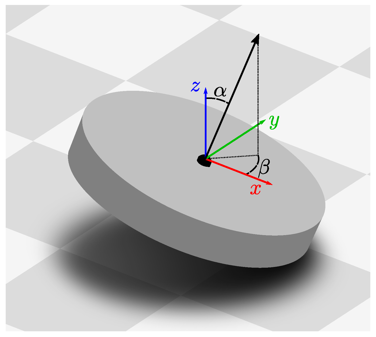
Figure 2.
The cleaning-robot prototype used to acquire the images used in this work. Images were captured with the panoramic camera, highlighted in the center. In this picture, the robot is shown without its cover.
Figure 2.
The cleaning-robot prototype used to acquire the images used in this work. Images were captured with the panoramic camera, highlighted in the center. In this picture, the robot is shown without its cover.

Figure 3.
An overview of the tilt-estimation pipeline used in this work. We use one of two different methods, which are shown on the left and right, respectively. First, a single panoramic camera image is edge-filtered (top). Next, edge pixels corresponding to vertical elements are identified (top left, right, shown in red). For the image-space method (Section 2.1), we approximate the tilt as a shifting of the edge pixels within the image. We estimate the shift direction and shift magnitude by fitting a function (bottom left, red line) to two parameters derived from the edge pixels (black dots). These parameters are based solely on the edge pixels’ positions and gradient directions in the image space. The vector-consensus method (Section 2.2) determines a 3D normal vector for each edge pixel. Each of these normals is orthogonal to the direction of the vanishing point. We then estimate this direction from a consensus of the normal vectors (bottom right, blue normals are orthogonal to tilt direction). Finally, we compute the tilt parameters from the shift or vanishing-point direction (bottom).
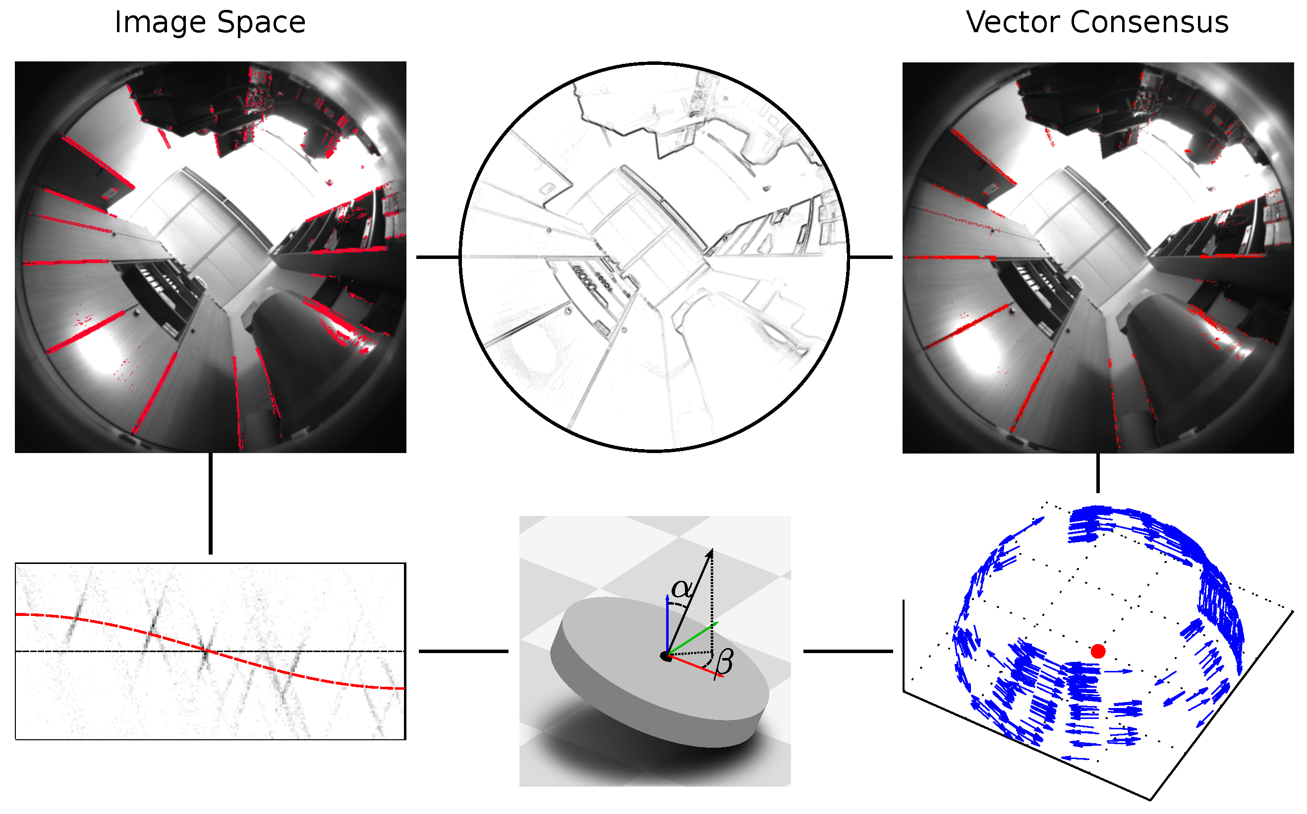
Figure 4.
An illustration of the vertical element’s vanishing point. This untilted image from our database shows a typical office environment. A blue dot represents the predicted vanishing point for an untilted robot . The red, dashed lines represent vertical elements, which we manually extended to their vanishing point (red ring, overlapping the blue dot). As expected, the predicted and actual vanishing point of the vertical elements are nearly identical.

Figure 5.
The result of the Scharr operator applied to the example image from Figure 4. The operator was only applied to a bounding box containing the pixels above the camera horizon. Black and white correspond to a strong dark-bright or bright-dark edge, respectively; gray indicates a weak edge response. We artificially increased the contrast of these images to make the gradients more noticeable.

Figure 6.
The same as Figure 4, but for a forward-tilted robot (). Due to the tilt, the approximated vanishing point (red dot) is shifted from (blue dot). Close inspection reveals that the tilt caused a slight curvature in the vertical lines. Thus, the dashed red lines and the resulting are merely an approximation of the true edges and vanishing point, respectively.

Figure 7.
The effect of tilts on image edges. This illustration shows the outlines of several cuboids, as seen by our robot’s camera. In Figure 7a, the robot is not tilted. The vertical elements appear as straight lines oriented towards a vanishing point (red dot). Figure 7b shows the effect of an exaggerated tilt, where vertical elements appear as curves. These curves no longer point straight towards the expected vanishing point (blue dot). This point has been shifted from its untilted position (red dot). This figure also contains the untilted outlines in a light shade of red. In the image-space method, we assume that small tilts do not cause the distortions in Figure 7b. Instead, we model the effect of such tilts as a mere shift in the image. This approximation is shown in Figure 7c, where the vanishing point and outlines are shifted without distortion.

Figure 8.
The camera model used in this work, which was first introduced by Scaramuzza et al. [34]. In Figure 8a, the point (red circle) lies at a bearing of (red arrow) relative to the camera center (black circle). A fisheye lens (light blue shape) projects onto the point (red circle) in an idealized sensor plane (gray square). This nonlinear projection is described by Equation (3) and the camera parameters from Equation (5). The distance between and the image center at is specified by . Applying Equation (4) to gives us the corresponding pixel coordinates in the actual digital image, as shown in Figure 8b. Here, the center of this image has the pixel coordinates .

Figure 9.
The parameters associated with an edge pixel k. In this illustration, the edge pixel is shown as a black square with position . This edge pixel has a gradient , represented by a black arrow. From this gradient, we calculate the gradient direction angle . The blue line indicates a hypothetical straight edge that is orthogonal to and passes through . This line also passes through the approximated vanishing point at (white disk). A tilt has shifted from the untilted vanishing point (gray disk). This shift is represented by a red line, and described by the angle and distance l. The distance between the blue line and is the edge offset from Equation (17). Finally, the angle between the blue and red lines is . Note that we model the effects of a tilt as a simple shift (Figure 7).

Figure 10.
The edge pixels from the prefiltered set F, which we extracted from the Scharr-filtered images in Figure 5. Valid edge pixels are shown in color, and are superimposed on the camera image. Figure 10a shows the untilted image from Figure 5, while Figure 10b shows the same location with a forward tilt. We reject pixels with bearings of more than 45° above the horizon, or with a gradient intensity of . Pixels with an edge offset were also rejected. In this visualization, the pixel’s hue indicates its gradient direction angle . The saturation represents the edge offset , with full saturation and desaturation corresponding to and , respectively. are the ground-truth tilt parameters calculated from the measured wheel heights (Section 2.3).

Figure 11.
The gradient direction angle and edge offset of the edge pixels shown in Figure 10. Edge pixels are shown as a 2D histogram, with darker bins containing more edge pixels. The red, dashed line shows the cosine predicted from the ground-truth tilt according to Section 2.1.3. A thin, dashed black line corresponds to . Due to noise and non-vertical elements in the environment, some edge pixels noticeably deviate from this ideal curve.
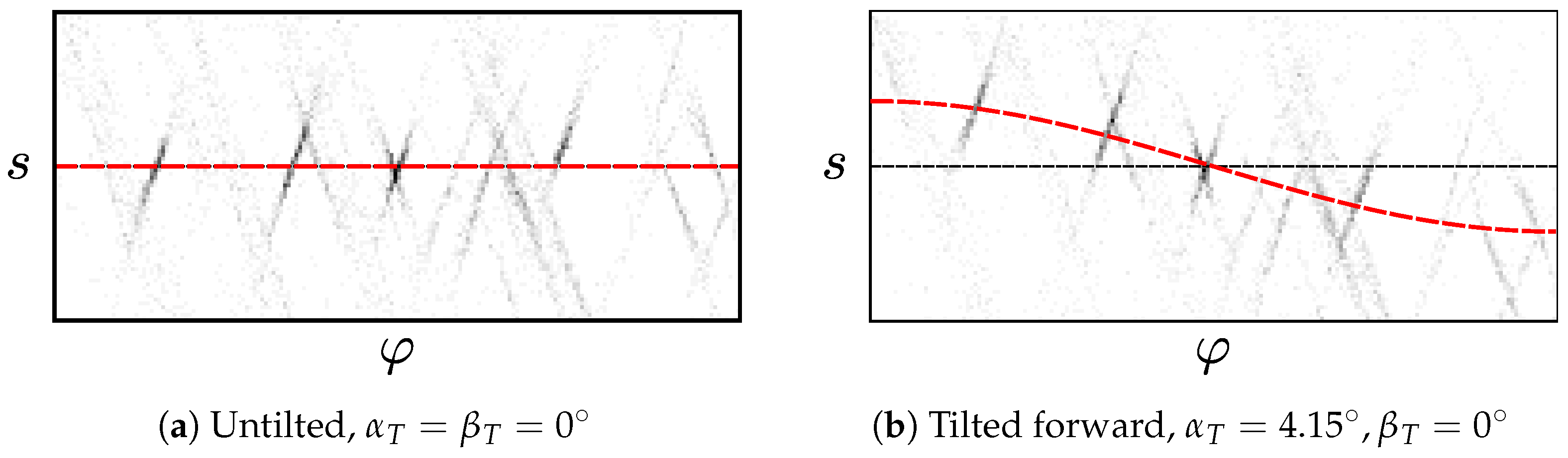
Figure 12.
The edge pixels from the image in Figure 13, visualized as in Figure 11. The blue line represents the cosine fitted to the edge pixels using least squares. In Figure 12a incorrect pixels were not rejected. There is a large error between the estimate (blue) and ground truth (red). Applying RANSAC with a threshold gives a much better result, shown in Figure 12b. Here, the histogram contains only the edge pixels remaining after RANSAC.
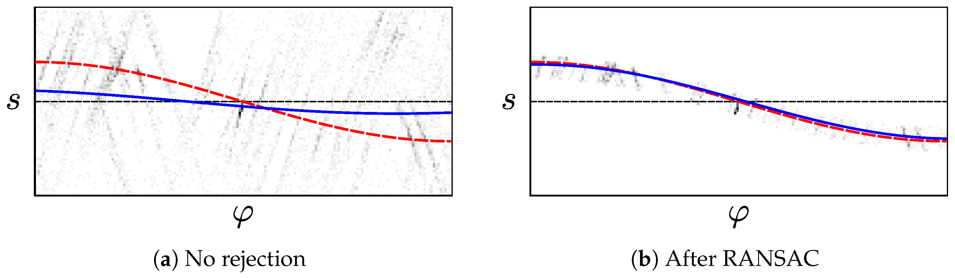
Figure 13.
Edge pixels after prefiltering, visualized as in Figure 10. This image includes numerous incorrect edge pixels. These are caused by near-vertical elements, such as parts of the curved chairs. If they are not rejected, these pixels cause errors in the least-squares tilt estimate. The camera image was captured with a forward tilt of .

Figure 14.
Using the reject-refit scheme to reject incorrect edge pixels from Figure 13. Edge pixels are visualized through histograms, as in Figure 12. Figure 14a shows the remaining edge pixels after the first two iterations. The error between the ground truth (red) and the curve fitted to the remaining pixels (blue) is reduced, compared to Figure 12a. Once the reject-refit scheme converges for , the error shown in Figure 14b is even lower.

Figure 15.
Vertical elements in the environment and their appearance in the camera image. In Figure 15a, the orientations for some elements are indicated by arrows. The robot’s movement plane is highlighted in red, with a black arrow representing the plane’s surface normal . Note that the and are parallel. Figure 15b shows the robot’s camera view in this location. The vertical elements from Figure 15a appear as straight edges. Colored circles represent the edge pixels that correspond to the vertical elements in Figure 15a. Each such pixel has a position and gradient vector ; the latter is shown by dashed lines. Since the camera image contains only the 2D projections of the 3D , we cannot determine these orientations directly.

Figure 16.
An environment element with orientation is projected onto an image plane (gray). This produces an edge pixel with position and gradient . is the 3D bearing vector associated with the image position , and similarly . The normal specifies the orientation of the blue plane that contains both and , this plane is only partially drawn as a triangle. We cannot fully determine from the projection and alone. Any element in the blue plane—such as or —would result in the same edge pixel. All vectors in this illustration are relative to the camera reference frame. Note that we use a linear camera as an approximation of the actual camera model from Figure 8: this is plausible because the projection is approximately linear within a small radius around the pixel : within this radius, , and thus Equation (3) is a linear projection.
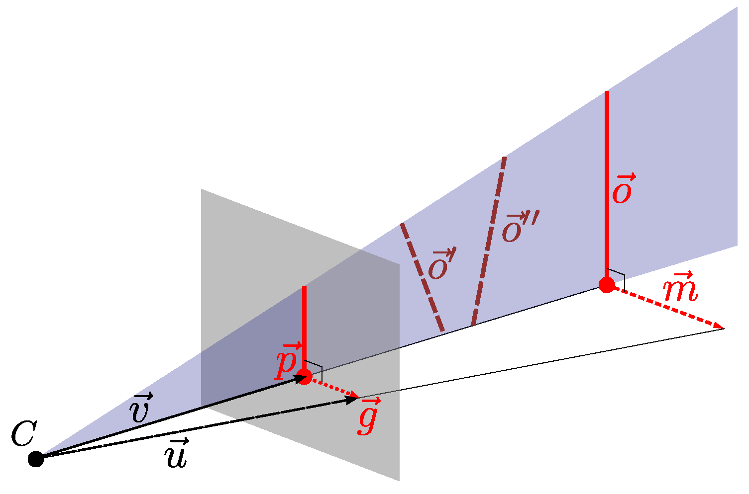
Figure 17.
The normal vectors of the edge pixels for an untilted robot. For the sake of clarity, only 500 randomly selected edge pixels are shown. Each edge pixel k is shown as a an arrow, with the orientation representing the normal vector . The base of each arrow lies along the bearing belonging to the pixel k. Figure 17a is based on the edge pixels extracted from the camera image in Figure 18a. As in Figure 18, we do not include edge pixels with a gradient intensity below . Figure 17b shows the result of prefiltering (°) and RANSAC (°). As expected for an untilted robot, the remaining are mostly orthogonal to the vertical axis remain.
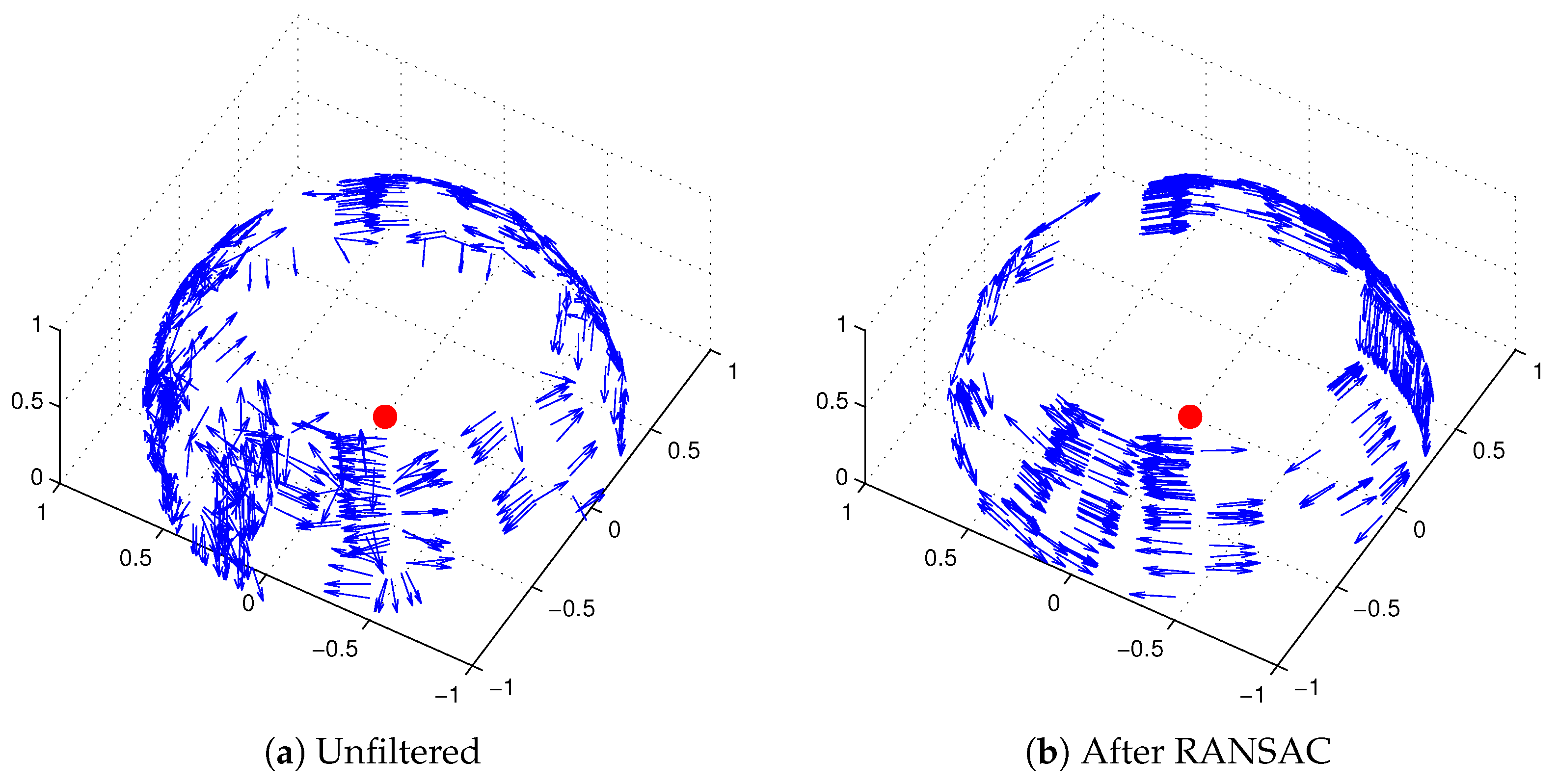
Figure 18.
Edge pixels corresponding to vertical elements, as identified through RANSAC. Edge pixels within the largest set are marked in red. The camera images are the same as used in Figure 10, cropped to the area above the horizon. Edge pixels with a gradient intensity below were discarded and are not shown. After prefiltering with °, we applied RANSAC with °.
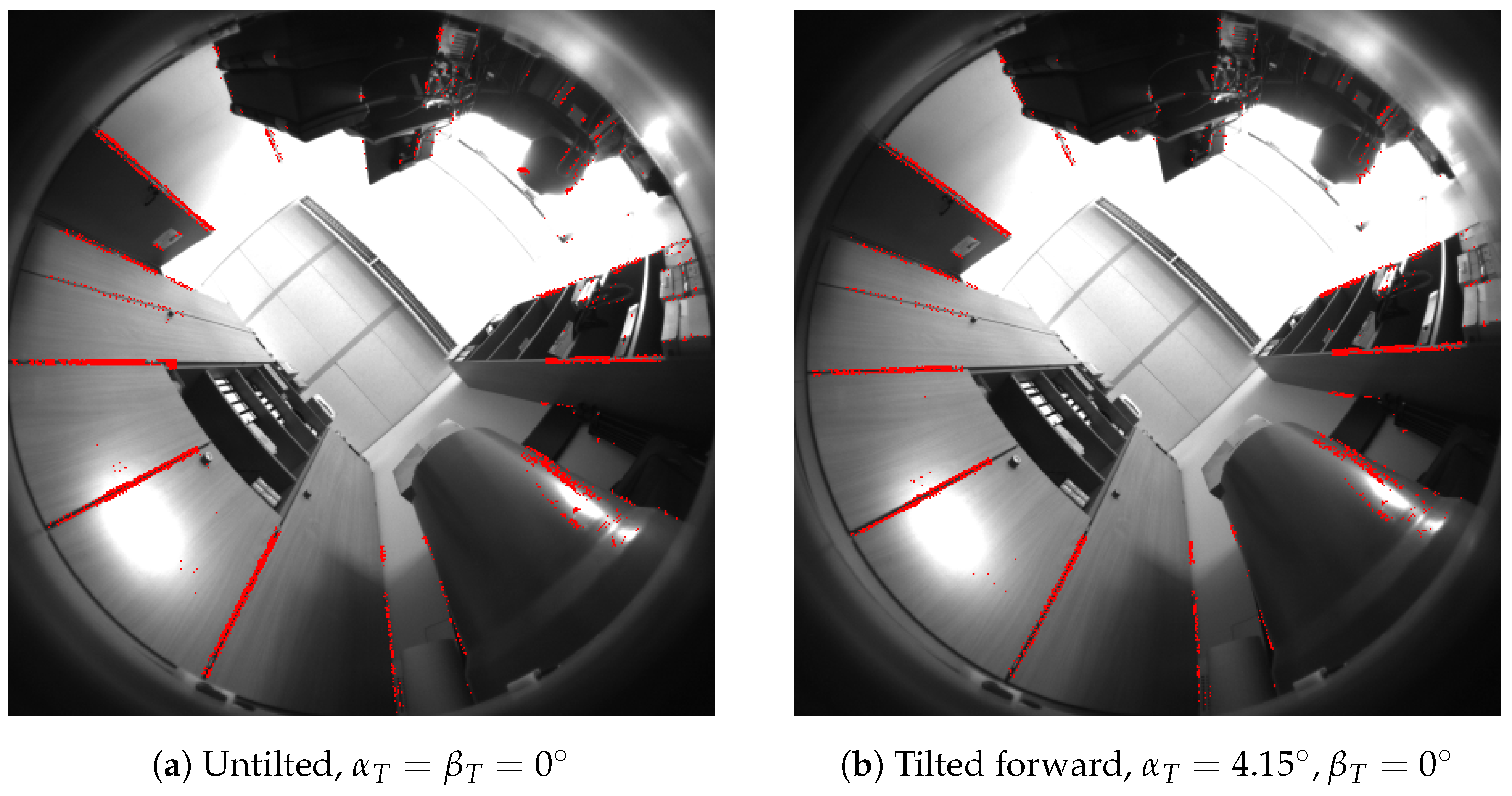
Figure 19.
The robot at three different locations from our image database. Besides open areas (Figure 19a), we also captured images in narrow spaces (Figure 19b) and beneath furniture (Figure 19c).

Figure 20.
The wheel layout of our cleaning-robot prototype. The panoramic camera (black circle) is mounted at the center of a ground plate (light gray). A red X marks the ground-contact points for each wheel, on which the robot rests. Relative to the center of the camera, the caster wheel’s (gray circle) contact point is at . The contact points of the left and right main wheel (gray rectangles) lie at , respectively. Here, we assume that the contact points are fixed and unaffected by tilts.

Figure 21.
The fraction of images for which the tilt-estimation error is . All curves were generated using the parameters from Table 3. For the sake of clarity, this figure was truncated to . We note that high errors can occasionally occur for all methods.
Figure 21.
The fraction of images for which the tilt-estimation error is . All curves were generated using the parameters from Table 3. For the sake of clarity, this figure was truncated to . We note that high errors can occasionally occur for all methods.

Figure 22.
The mean tilt-estimation error , depending on the true tilt angle . The pale, dotted or dash-dotted lines represent each method’s across all images. As in Figure 21, we used the parameters from Table 3. The ground-truth tilt angle was calculated using Equation (42).
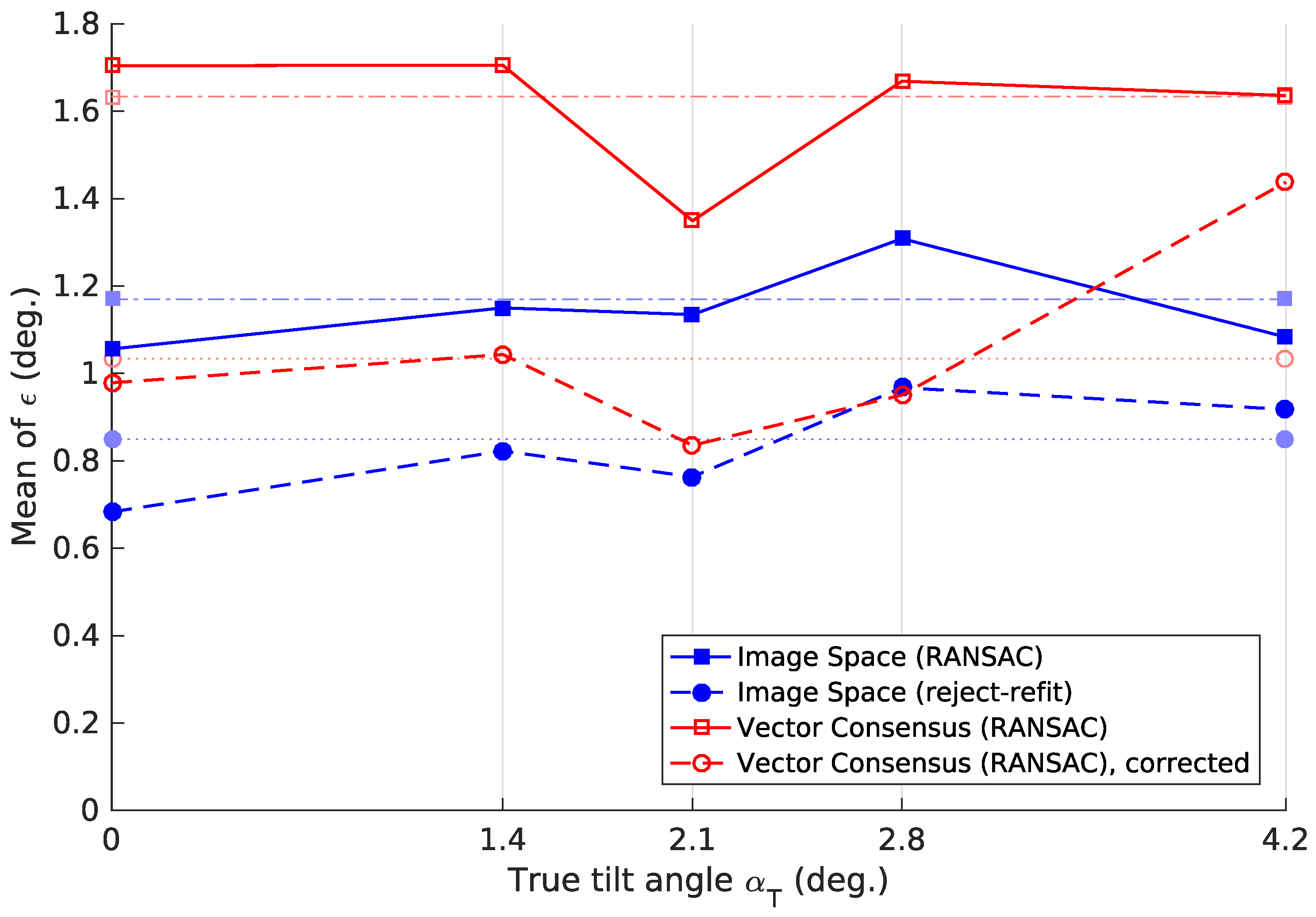
Figure 23.
The mean tilt-estimation error for each of the six environments. The methods and parameters used were the same as in Table 3. The pale, dotted or dash-dotted lines represent each method’s across all images. Although there is some variation, each method’s tilt-estimation results are broadly similar across the different environments.
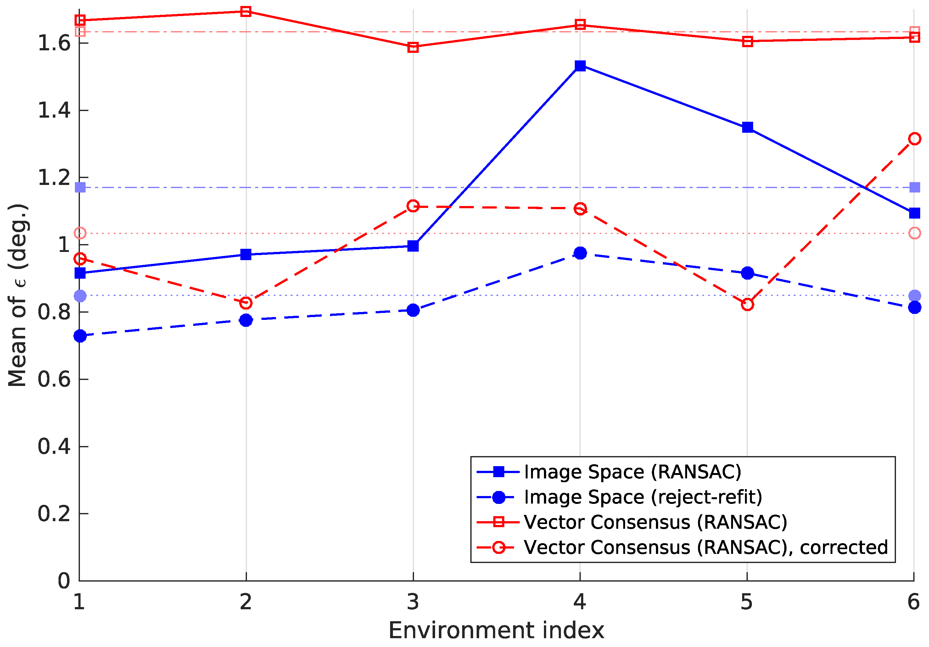
Figure 24.
The mean tilt-estimation error , plotted against the mean execution time. The time was measured on the modern desktop system, as described in Section 2.4. Each point represents one parameter combination from Table 2. The points with the lowest from Table 3 are highlighted in black. As shown here, accepting a slightly higher can sometimes notably reduce the execution time. We limit this figure to ° and . This causes a few points to be omitted, but greatly improves legibility.

Figure 25.
This variant of Figure 24 shows the results for the embedded system described in Section 2.4. Similar to Figure 24, we limit this figure to ° and .
Figure 25.
This variant of Figure 24 shows the results for the embedded system described in Section 2.4. Similar to Figure 24, we limit this figure to ° and .
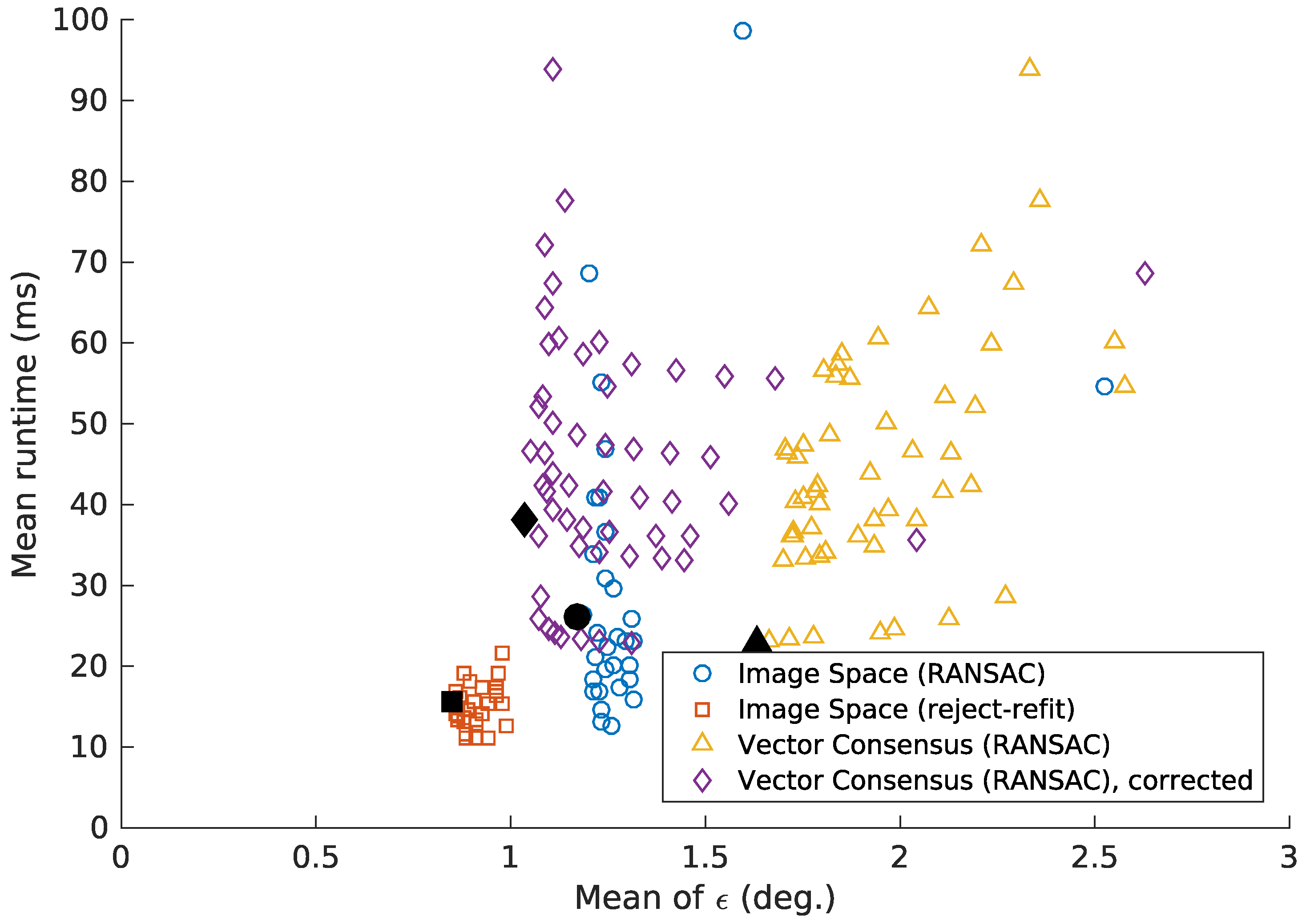
Figure 26.
The effect of the tilt angle on the orientation and bearing error in visual pose estimation. For the planar-motion Min-Warping method [10], the pose-estimation errors (blue lines) increase with the tilt angle. In contrast, the red lines show constant errors for a nonplanar method [14] with local visual features [48]. Gray lines mark the tilt angle beyond which the planar-motion error exceeds the nonplanar one; this occurs at about °. This figure is based on results from an earlier work, which contains additional details (Figure 19) [1].
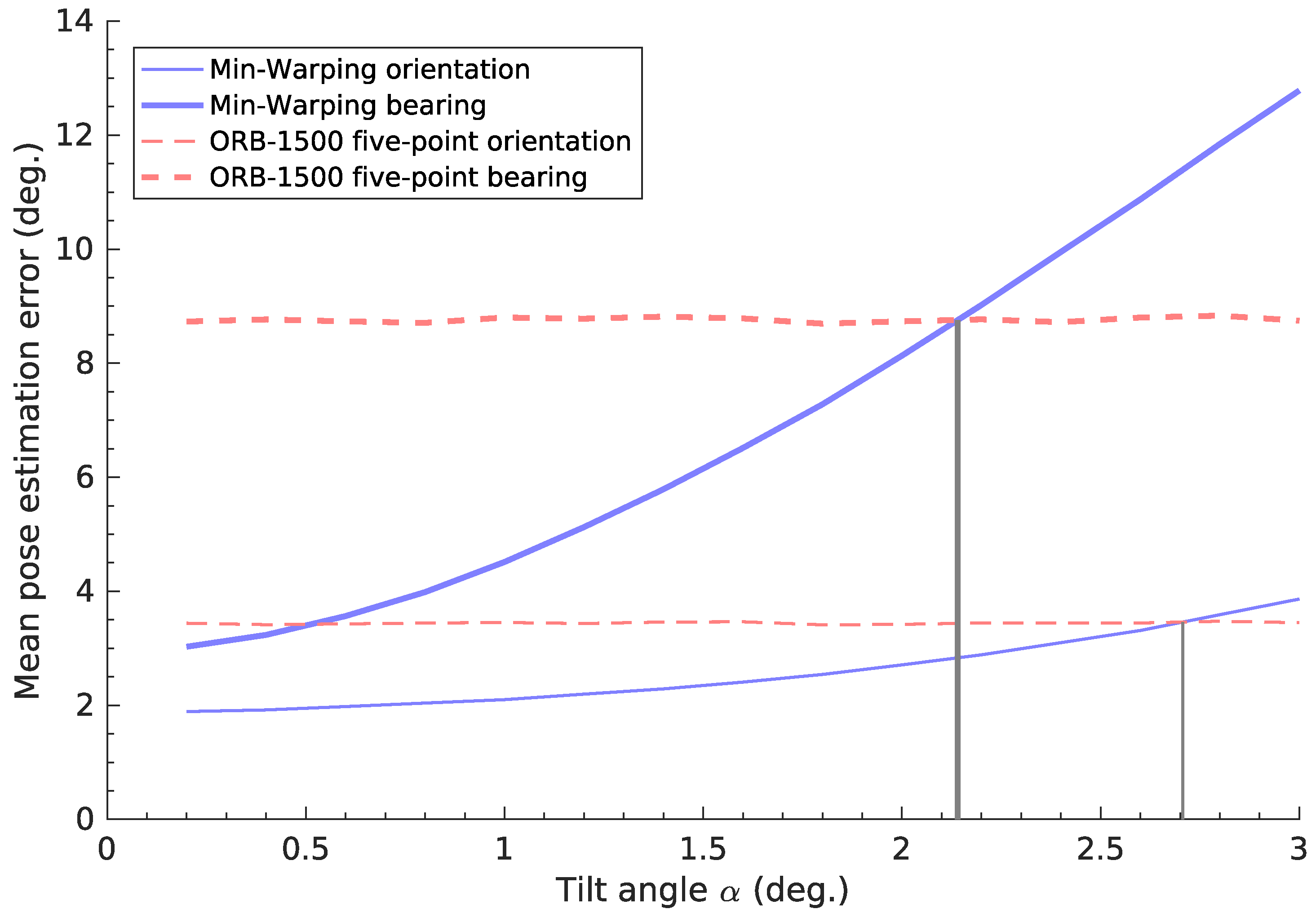
Figure 27.
Figure 27a shows a forward-tilted image (°) captured at the location in Figure 19c. As in Figure 10, the prefiltered edge pixels are highlighted in color. Few of these edge pixels correspond to vertical elements, while incorrect edge pixels are common. Similar to Figure 11, we visualize the parameters of the edge pixels in Figure 27b. A dashed red line shows the expected relationship between and s for edge pixels from vertical elements. Unlike in Figure 11, few of the edge pixels actually lie close to this line. The solid blue line shows the curve for the incorrect estimated by the reject-refit scheme. While it is a poor tilt estimate, the curve is a better fit for the in the histogram. Thus, the poor tilt estimate is likely caused by the incorrect edge pixels. The RANSAC-based estimate suffers from a similar error, as illustrated by the dotted blue line.

Figure 28.
The true and estimated tilt angle for corrected and uncorrected estimates. For each method, we used the parameters (Table 3) that minimize after correction. This figure was generated using the factors and for each image location L, which we determined according to Section 2.4. For the uncorrected image-space method, we calculated using Equation (26). A black line represents a perfect match between and .


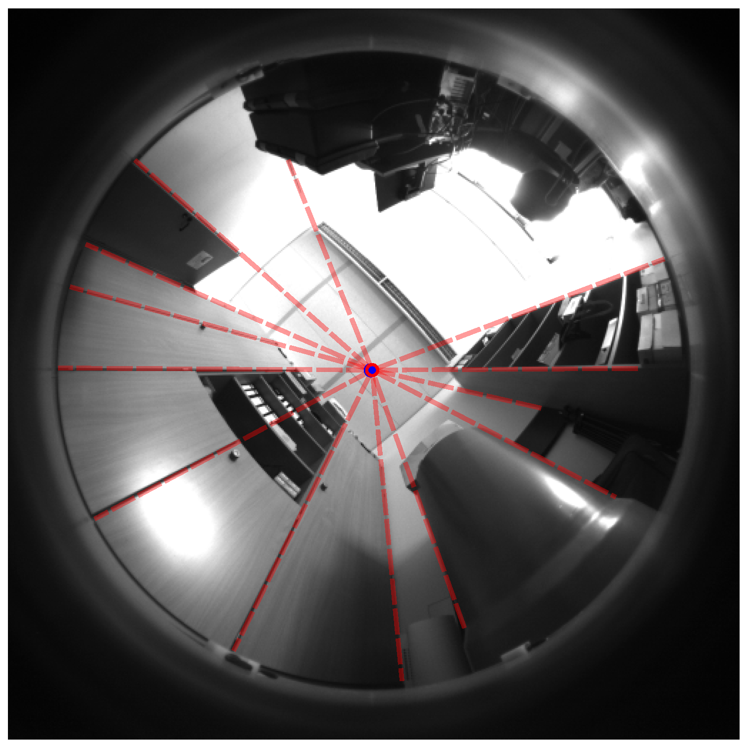
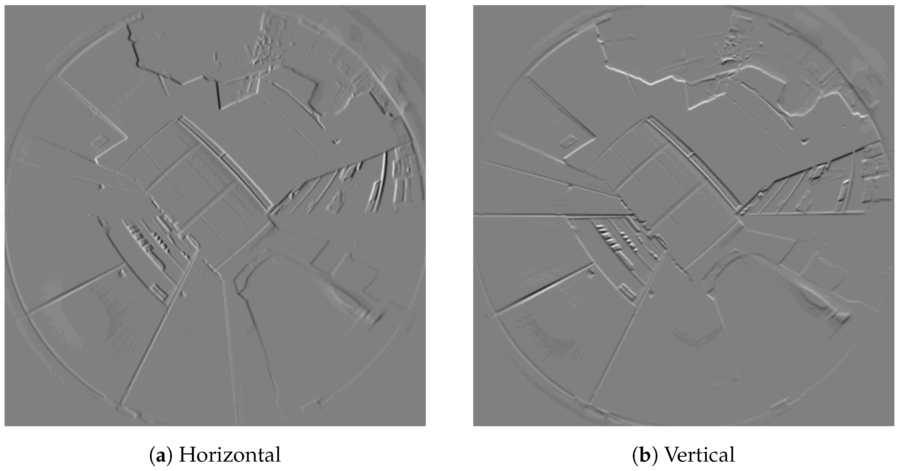
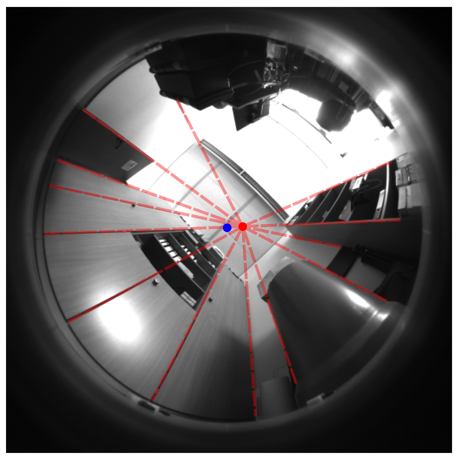
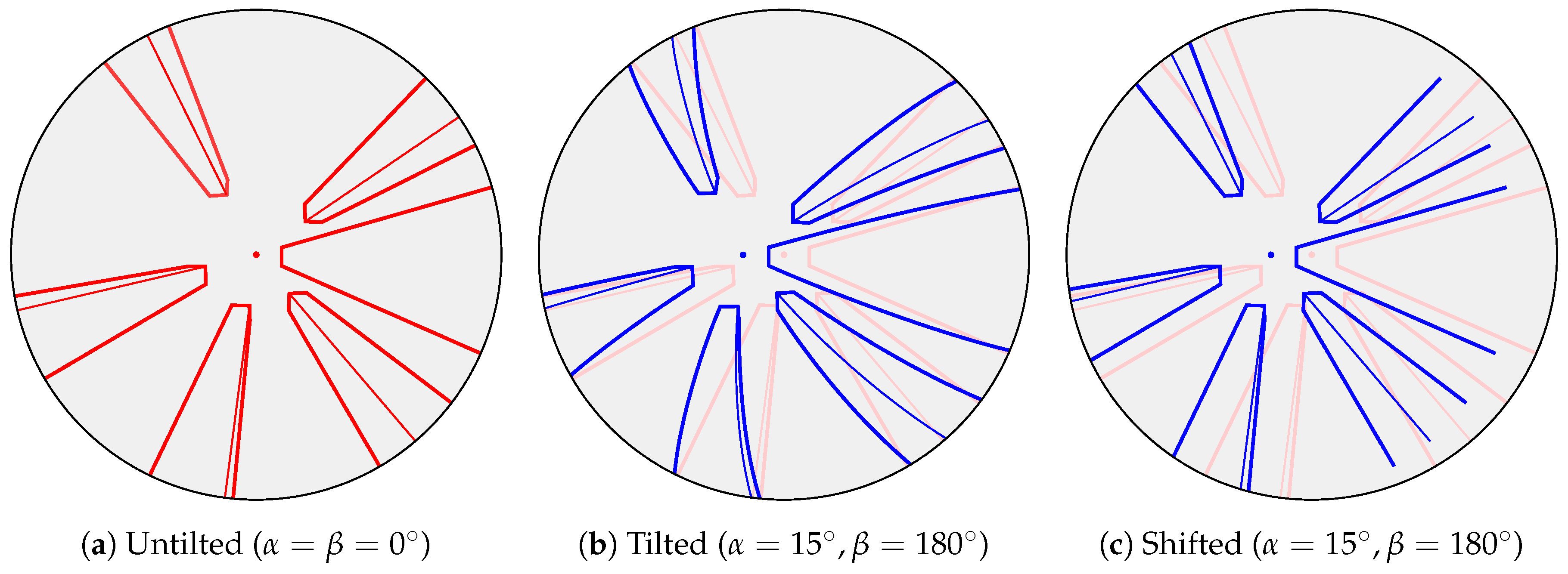
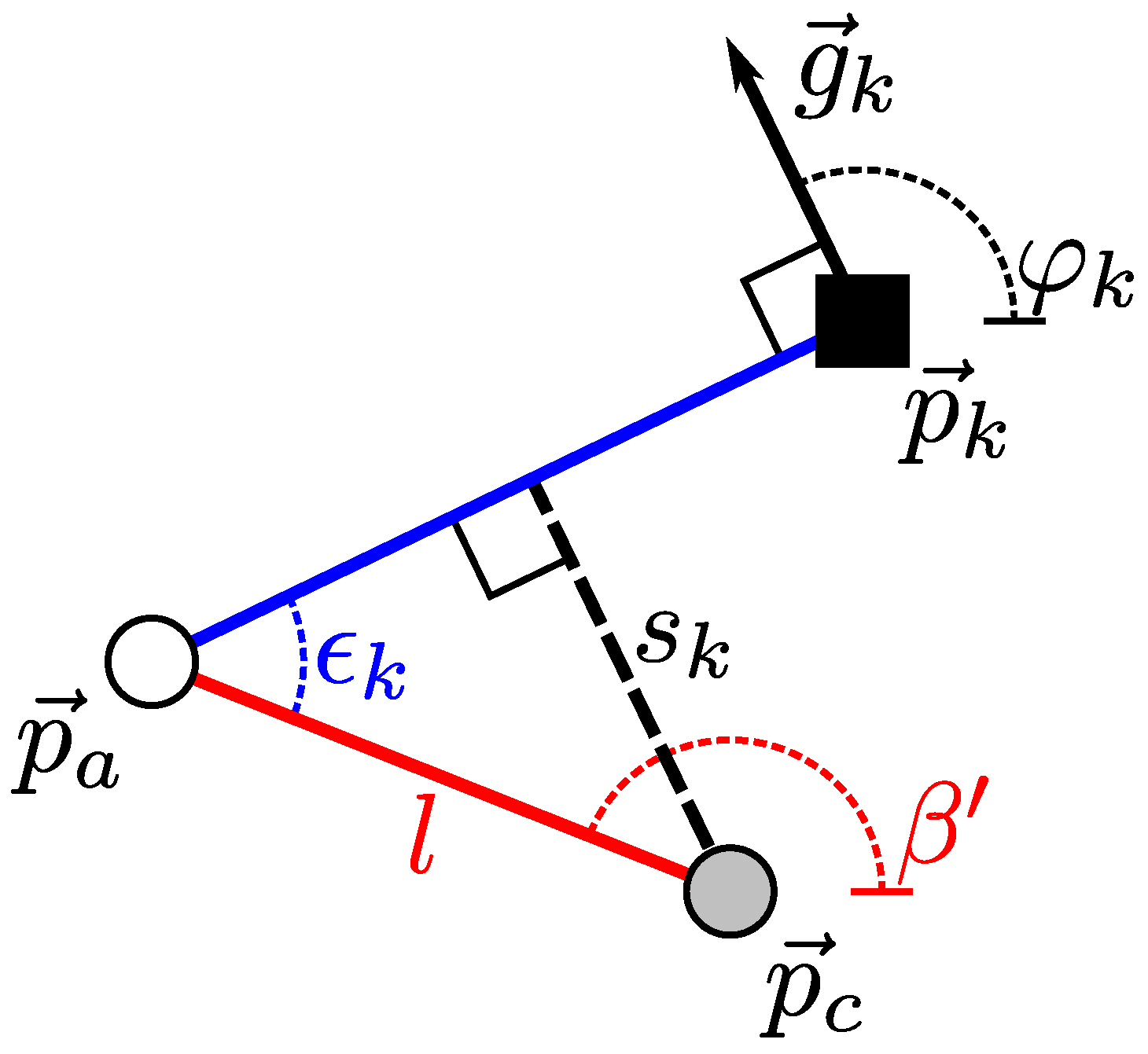
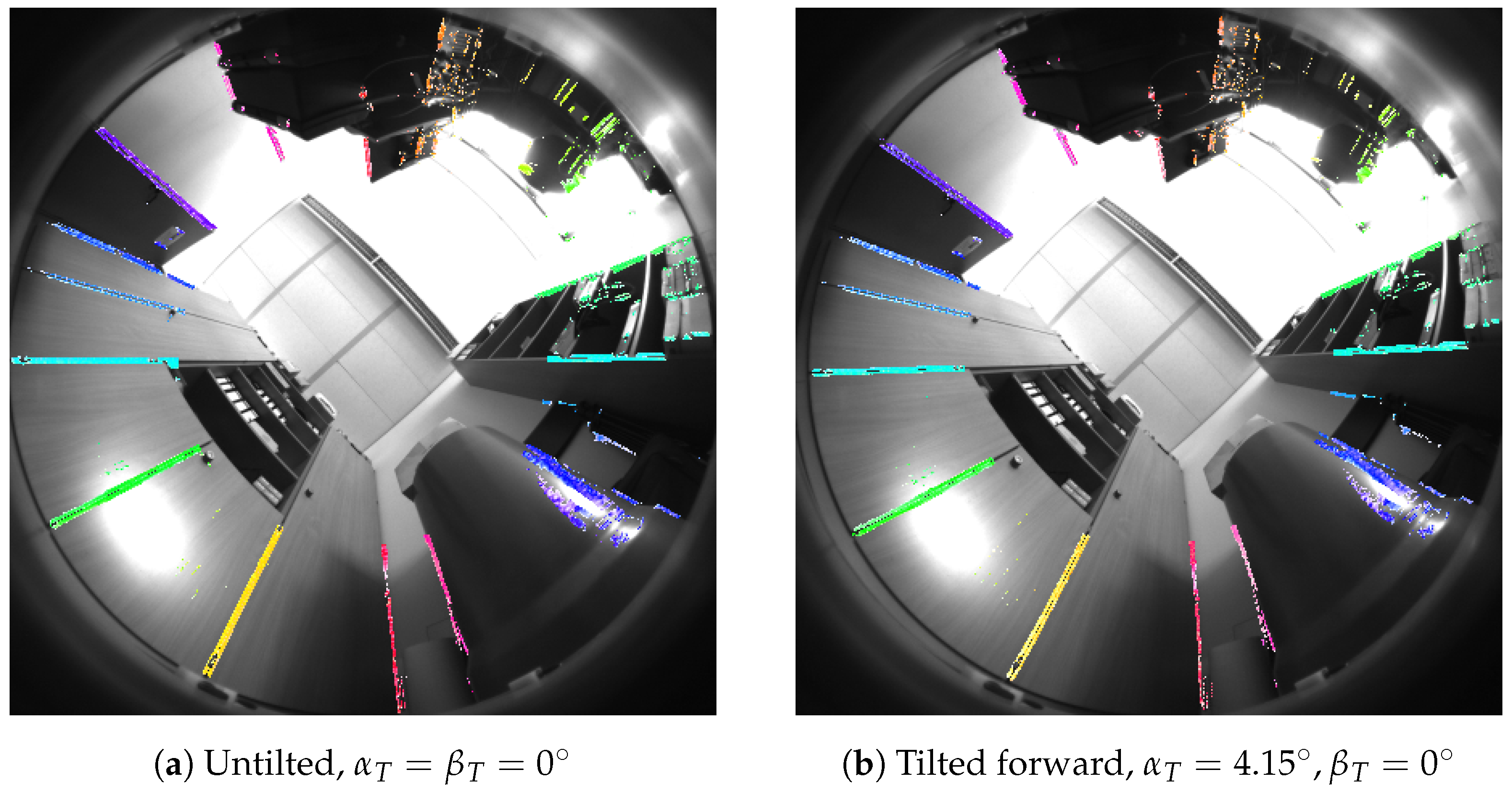
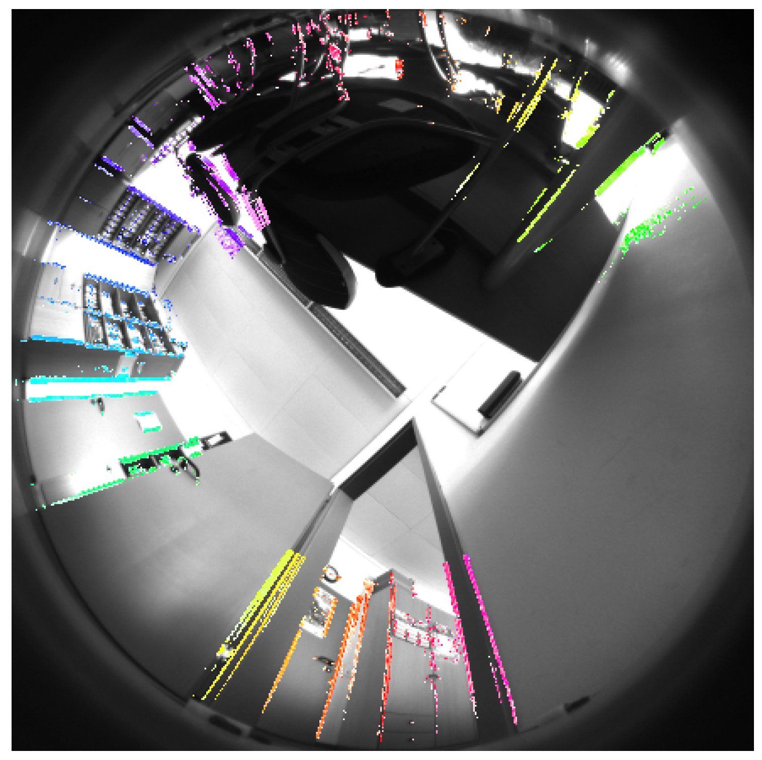
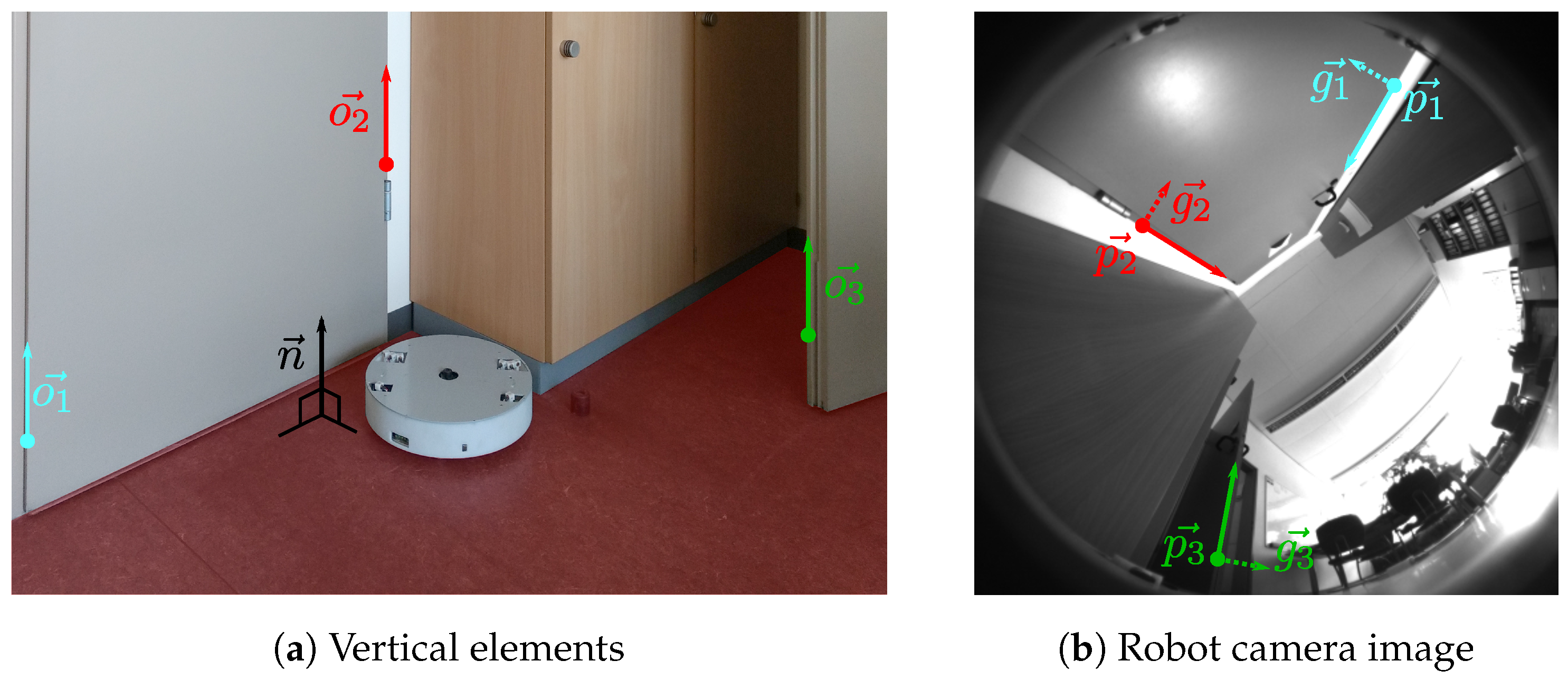
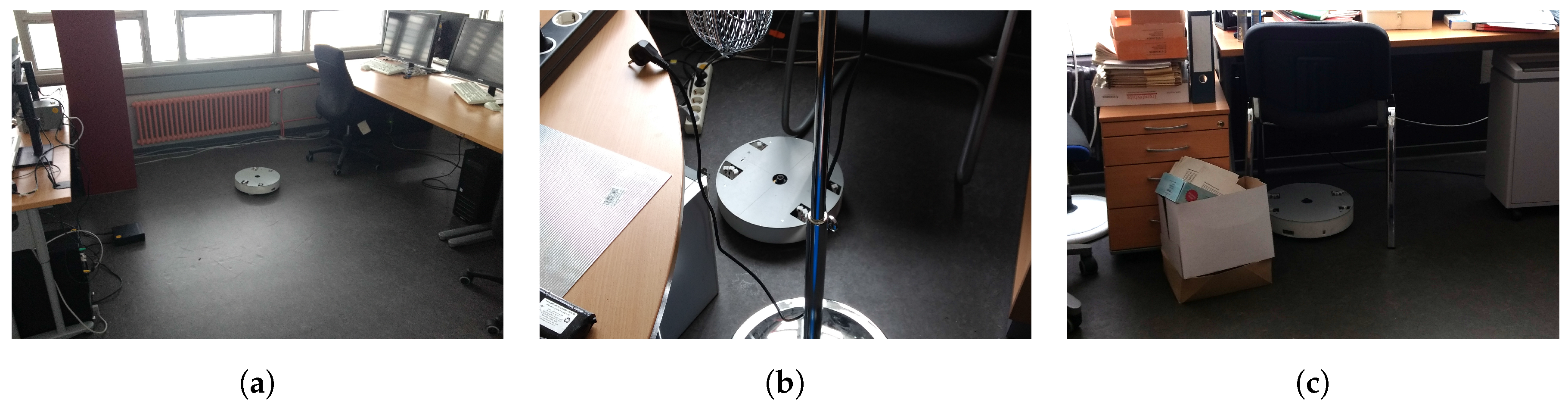
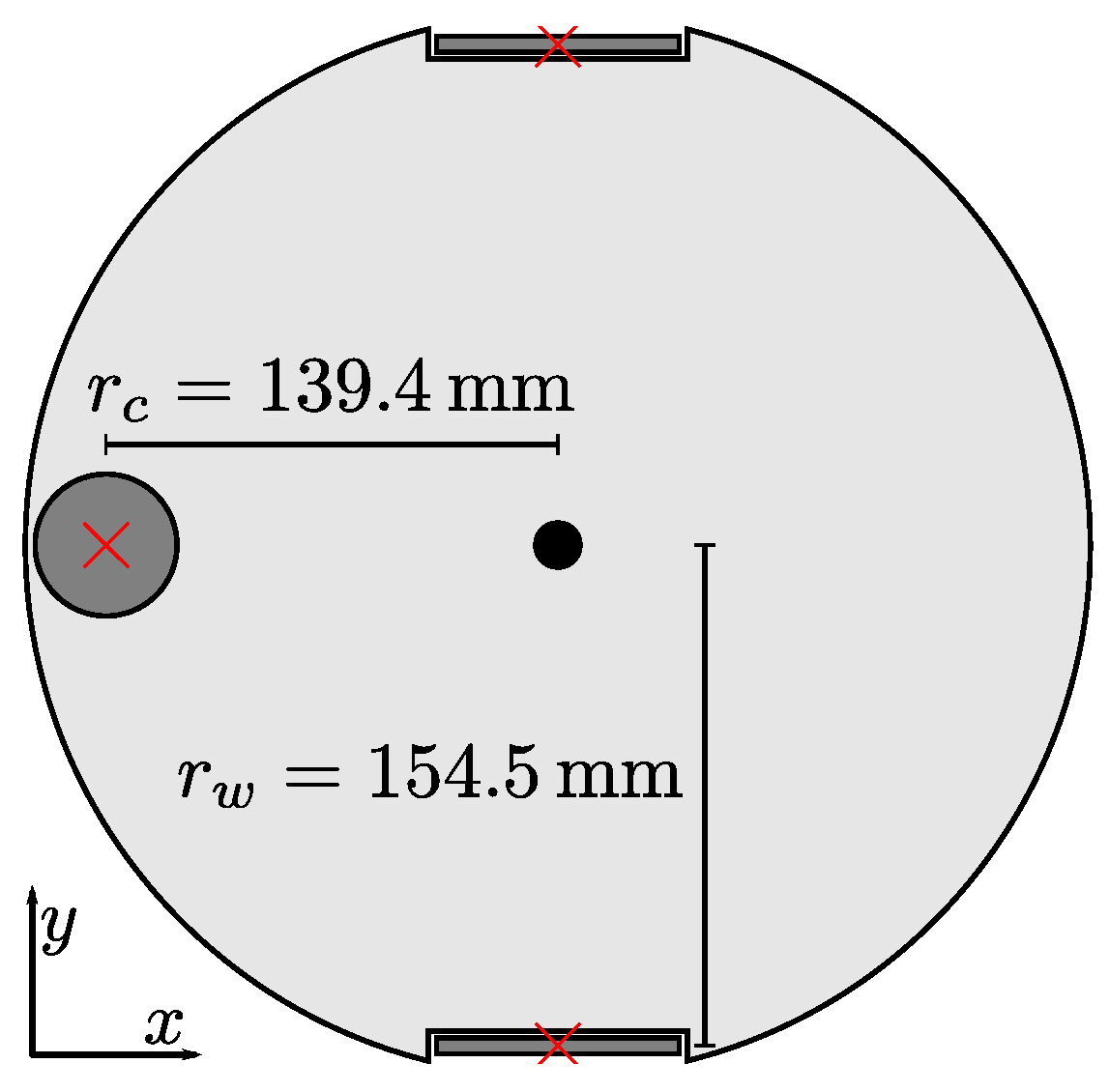
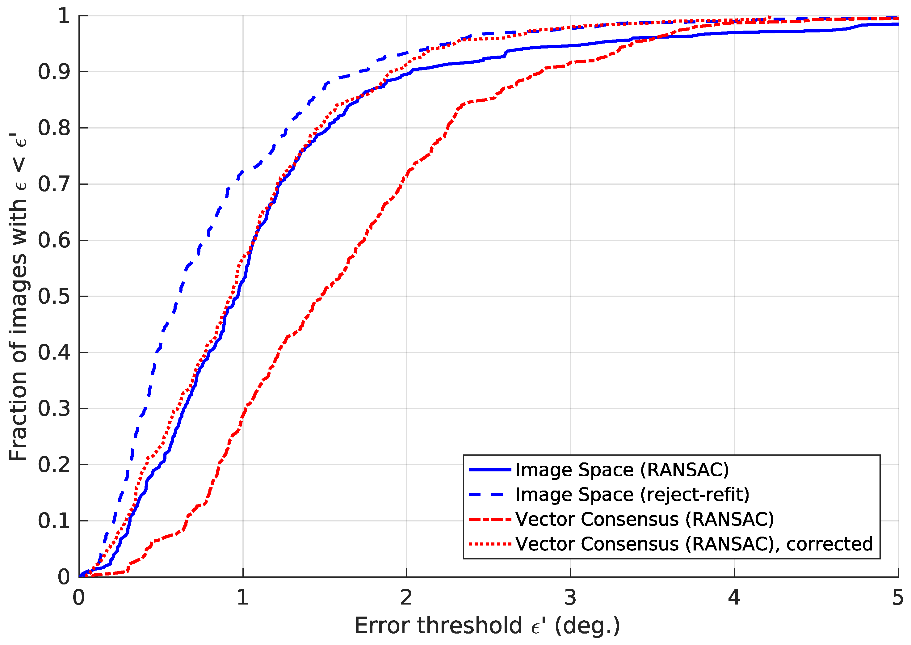
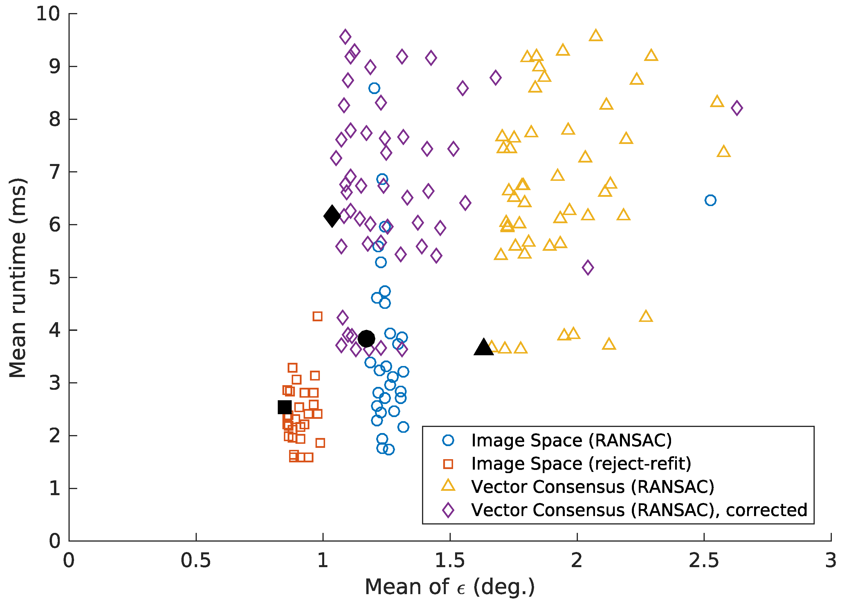
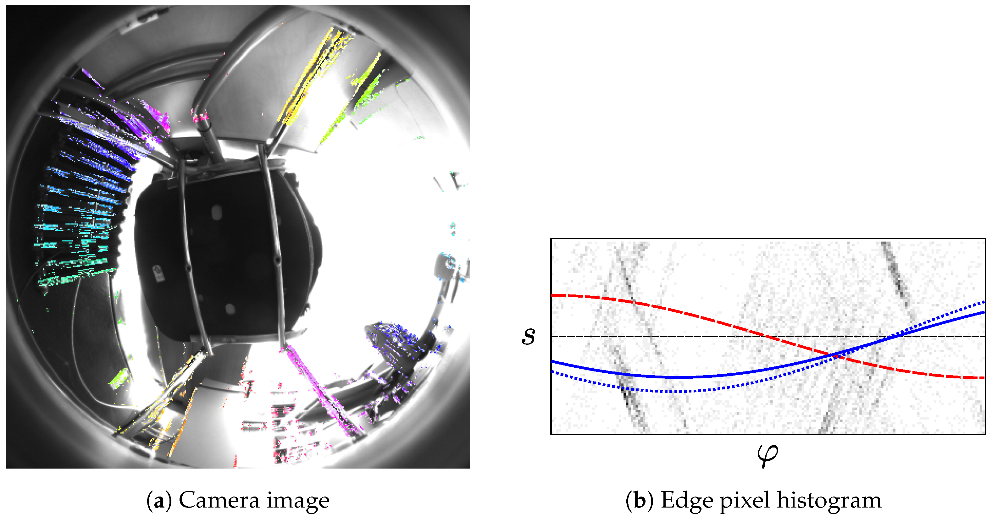
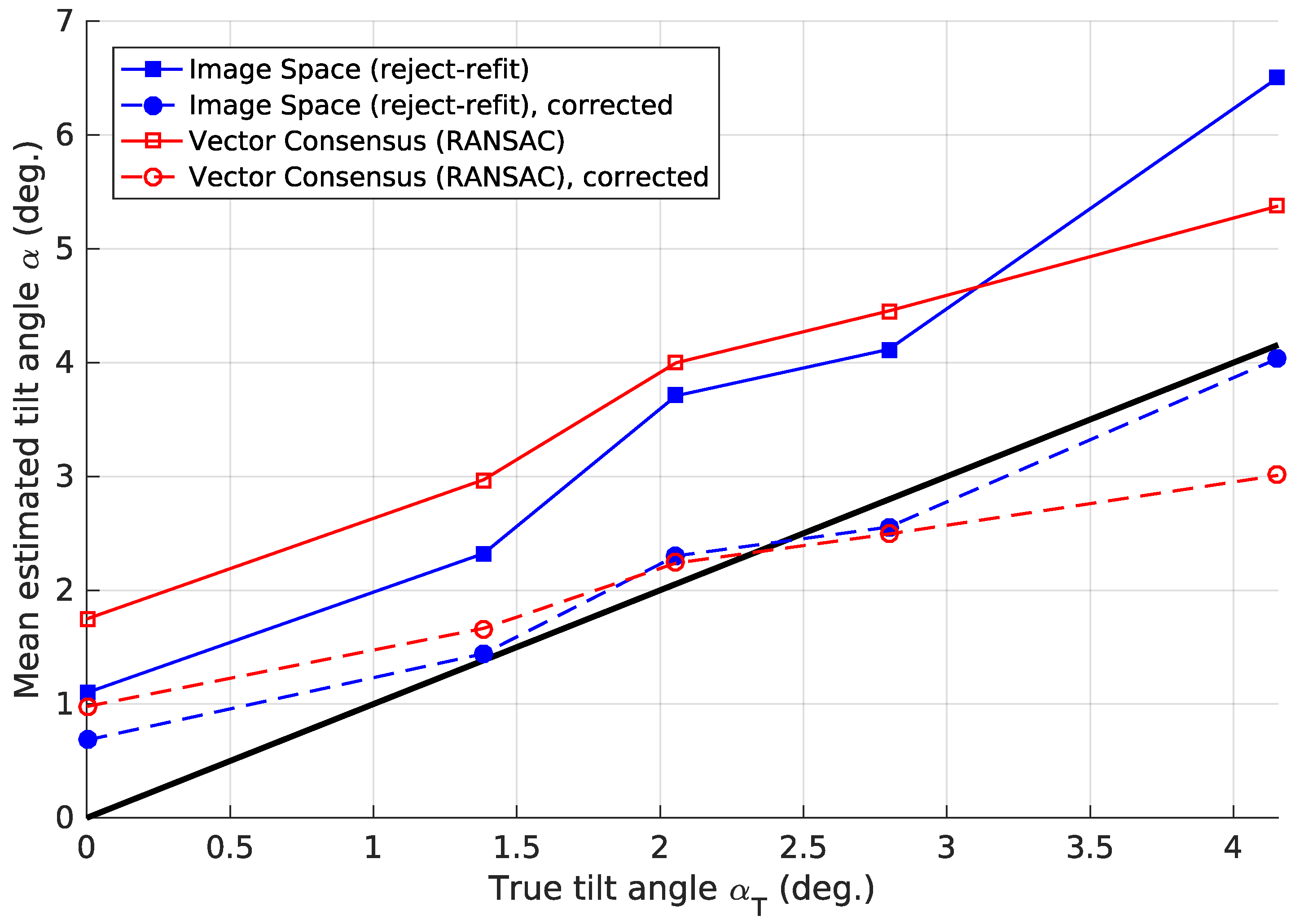
Table 1.
The ground-truth tilt angle when raising one wheel by a distance h, as calculated from Equation (42). Raising one of the main wheels results in ° for the left and right wheel, respectively (Equation (43)). ° when raising the caster wheel, which holds up the rear of the robot. Spacer refers to the metal spacers used to capture tilted images. We also included common objects from a domestic environment that may cause the robot to tilt. The values in this table were calculated for a stationary robot. For a moving robot, driving-related forces or torques may affect the true tilt angle or direction.
| Object | h | (Main Wheel) | (Caster) |
|---|---|---|---|
| Spacer (thin) | 5.0 mm | 1.38° | 2.06° |
| Spacer (thick) | 10.1 mm | 2.80° | 4.15° |
| Carpets (various) | 4.4 mm to 7.4 mm | 1.22° to 2.05° | 1.81° to 3.04° |
| Door threshold | 5.3 mm | 1.47° | 2.18° |
Table 2.
Parameter values evaluated in our experiments. Depending on the method and variant used, each value for was tested with all other values for Q, , and . This results in combinations for , for , and for .
Table 2.
Parameter values evaluated in our experiments. Depending on the method and variant used, each value for was tested with all other values for Q, , and . This results in combinations for , for , and for .
| Parameter | Values Tested |
|---|---|
| Gradient intensity threshold | 100, 150, 200, 250, 300, 600 |
| Rejection fraction Q | 0.5, 0.7, 0.8, 0.9 |
| Random Sample Consensus (RANSAC) threshold | 2.5, 5, 7.5, 10, 12.5, 15 pixels |
| RANSAC threshold | 0.5°, 1°, 1.5°, 2°, 2.5°, 3°, 3.5°, 4°, 4.5°, 5° |
Table 3.
The mean tilt-estimation error and standard deviation for the methods and variants being tested. The last line lists the vector-consensus results achieved when correcting the estimated tilt angle using the factor (Section 2.4). For each method, we only list the results for the parameters given in the third column. Out of the possibilities from Table 2, these values gave the lowest . We also included the 50th percentile (median) and 95th percentile of .
| Method | Variant | Parameters | Estimation error (°) | ||
|---|---|---|---|---|---|
| () | 50% | 95% | |||
| Image Space | RANSAC | , | 1.17 (1.03) | 0.97 | 3.16 |
| reject-refit | , | 0.85 (0.81) | 0.61 | 2.27 | |
| Vector Consensus | RANSAC | , ° | 1.63 (0.93) | 1.48 | 3.38 |
| ”, corrected | , ° | 1.03 (0.72) | 0.92 | 2.30 | |
Table 4.
The time required for tilt estimation, calculated according to Section 2.4. This table lists the mean, standard deviation and 50th (median) and 95th percentile, in milliseconds. Times are given for the modern desktop CPU, as well as the embedded CPU carried by our robot prototype. Each method used the parameters listed in Table 3, which gave the lowest mean error . Note that the corrected vector-consensus method appears to be much slower than the uncorrected variant. This is not due to the correction step, which consumes little time. Instead, the corrected variant achieves its lowest for different parameter values (Table 3). However, these values also lead to longer execution times. Compared to the uncorrected variant, the corrected variant actually gives better in similar time (Figure 24 and Figure 25).
| Method | Variant | Desktop (ms) | Embedded (ms) | ||||
|---|---|---|---|---|---|---|---|
| Mean () | 50% | 95% | Mean () | 50% | 95% | ||
| Image Space | RANSAC | 3.8 (1.43) | 3.7 | 6.3 | 26.0 (6.89) | 25.2 | 41.8 |
| reject-refit | 2.5 (0.85) | 2.5 | 4.1 | 15.7 (3.02) | 15.3 | 20.7 | |
| Vector Consensus | RANSAC | 3.6 (1.22) | 3.5 | 5.7 | 22.9 (4.69) | 23.2 | 29.4 |
| corrected | 6.2 (1.88) | 6.0 | 9.3 | 38.1 (9.72) | 36.9 | 51.8 | |
© 2017 by the author. Licensee MDPI, Basel, Switzerland. This article is an open access article distributed under the terms and conditions of the Creative Commons Attribution (CC BY) license (http://creativecommons.org/licenses/by/4.0/).
Share and Cite
MDPI and ACS Style
Fleer, D. Visual Tilt Estimation for Planar-Motion Methods in Indoor Mobile Robots. Robotics 2017, 6, 32. https://doi.org/10.3390/robotics6040032
AMA Style
Fleer D. Visual Tilt Estimation for Planar-Motion Methods in Indoor Mobile Robots. Robotics. 2017; 6(4):32. https://doi.org/10.3390/robotics6040032
Chicago/Turabian StyleFleer, David. 2017. "Visual Tilt Estimation for Planar-Motion Methods in Indoor Mobile Robots" Robotics 6, no. 4: 32. https://doi.org/10.3390/robotics6040032
Note that from the first issue of 2016, this journal uses article numbers instead of page numbers. See further details here.