Human-Like Room Segmentation for Domestic Cleaning Robots

Computer Engineering Group, Faculty of Technology, Bielefeld University, D-33594 Bielefeld, Germany
Robotics 2017, 6(4), 35; https://doi.org/10.3390/robotics6040035
Submission received: 20 October 2017
/
Revised: 22 November 2017
/
Accepted: 23 November 2017
/
Published: 26 November 2017
Abstract
:Autonomous mobile robots have recently become a popular solution for automating cleaning tasks. In one application, the robot cleans a floor space by traversing and covering it completely. While fulfilling its task, such a robot may create a map of its surroundings. For domestic indoor environments, these maps often consist of rooms connected by passageways. Segmenting the map into these rooms has several uses, such as hierarchical planning of cleaning runs by the robot, or the definition of cleaning plans by the user. Especially in the latter application, the robot-generated room segmentation should match the human understanding of rooms. Here, we present a novel method that solves this problem for the graph of a topo-metric map: first, a classifier identifies those graph edges that cross a border between rooms. This classifier utilizes data from multiple robot sensors, such as obstacle measurements and camera images. Next, we attempt to segment the map at these room–border edges using graph clustering. By training the classifier on user-annotated data, this produces a human-like room segmentation. We optimize and test our method on numerous realistic maps generated by our cleaning-robot prototype and its simulated version. Overall, we find that our method produces more human-like room segmentations compared to mere graph clustering. However, unusual room borders that differ from the training data remain a challenge.
1. Introduction
Domestic tasks such as cleaning are a common application for autonomous mobile robots. To enable navigation and planning during such a task, a robot may build and use a map of its environment. This environment typically consists of rooms interconnected by passageways. For domestic robots, segmenting such a map into its component rooms has multiple uses, including the following: first, the robot can refer to rooms when communicating with humans [1,2]. A user may give instructions that reference rooms, such as “Robot, move to the kitchen”. (This also requires room labeling, a step which we do not consider here.) Second, room segmentation can be a component in place categorization by integrating information [3,4]: for example, camera images captured at many points within the same room may be combined in an attempt to categorize the room. Third, room segmentation commonly plays a role in semantic mapping and multi-level planning (survey: [5]); for our floor-cleaning robot, hierarchical cleaning and user-defined cleaning plans are of special interest. However, ambiguous passageway- and room-like elements within the environment make discovery of this room structure nontrivial.
In this work, we present a novel method for human-like room segmentation in topo-metric maps. Specifically, we want to assign a room label to each node in the map graph. Nodes with the same label should be part of the same room. Ideally, the resulting rooms reproduce the judgment of a human observer. In brief, our method accomplishes this by performing four major steps: first, we preprocess the topo-metric map generated by our cleaning-robot, preparing it for segmentation. Second, we use the robot’s sensor data to calculate a feature vector for every edge in the map graph. Features are based solely on the immediate vicinity of an edge, and thus require no global map consistency. In a third step, a classifier uses these features to estimate whether or not a map edge crosses a room border. Finally, we apply a graph-clustering step to segment the map graph into rooms, taking into a account the room borders identified in the previous step.
The rest of this work is structured as follows: first, we discuss related works in Section 1.1, and compare them to our work in Section 1.2. Next, Section 2 describes our method in detail, elaborating on the four steps listed above. We then test our method across numerous environments using several experiments, as reported in Section 3. In Section 4, we discuss the results based on numerical quality measures, as well as examples of room segmentation results. Finally, Section 5 contains our conclusions, together with an outlook on possible future developments.
1.1. Related Work
In the literature, there are several works addressing the problem of room segmentation within the context of mobile robots. For this overview, we are especially interested in approaches overlapping with the one we propose in Section 2. Here, we distinguish between two different approaches to room segmentation: those from the first category perform place categorization, assigning labels such as office or kitchen. Such methods go beyond simple room segmentation, constructing semantic maps instead. However, the general problem of semantic mapping lies beyond the scope of this work. For a broader overview of semantic mapping for mobile robotics, we point to the survey by Kostavelis and Gasteratos [5]. Here, we focus on those semantic mapping works for which room segmentation is a central aspect. Conversely, members of the second category merely determine which map locations lie within the same room. They do not perform place categorization, and thus do not require information about potential place types.
1.1.1. Place Categorization
Methods from the first category commonly use a bottom-up approach: Here, a classifier determines which type of room surrounds a given place, based on sensor data the robot recorded at that point. For example, Mozos et al. [3] distinguish corridors, rooms, and doorways by applying a boosting classifier to features extracted from laser range scans. The authors apply this scheme to simulated scans generated from an occupancy grid map to classify the map’s cells. Connected cells with the same label are then joined together into regions, thus accomplishing room segmentation.
Friedman et al. [6] introduce Voronoi Random Fields (VRF) to segment occupancy grid maps. The authors extract a Voronoi graph from the map, and then use Conditional Random Fields (CRF) to assign labels such as hallway, room, doorway, or junction to each node. These labels are chosen based on the obstacles in the vicinity of each node, as well as the information encoded in the Voronoi graph. Grouping contiguous nodes with the same label then segments the map. Shi et al. [7] combine CRF with Support Vector Machines (SVM) to label the nodes of a generalized Voronoi graph based on simulated laser scans. Both the Voronoi graph and the laser scans were generated from occupancy grid maps. Here, the place types are more specific to the environment, for example cubicle, kitchen, or printer room.
Pronobis et al. [8] combine range scans with global [9] and local visual features [10] extracted from camera images. The authors apply separate classifiers to these features, using one multi-class Support Vector Classifier (SVC) for each of the three feature types. A final SVC combines these feature-specific results into a single place label. These labels are comparatively fine-grained, such as meeting room, office, or corridor. The authors then accumulate results from close-by locations to label entire areas, producing a room segmentation. In a subsequent work [11], place types are defined by their properties. These include a place’s geometric shape and size, as well as the types of nearby objects detected with a camera.
Ranganathan and Lim [12] utilize image sequences captured by a robot to label the cells of a grid representation. They use the PLISS (Place Labeling through Image Sequence Segmentation) system [13] to determine the probability that an image in a sequence depicts a certain type of place. In a novel approach, the authors then update the probabilities of those grid cells visible in the image, instead of the cell at which the image was taken. Occasional misclassifications are smoothed out by applying Conditional Random Fields to the grid. This work also uses fairly specific place labels, such as lab or printer room.
Some techniques use a room segmentation heuristic as a preprocessing step for semantic mapping. Zender et al. [14] apply the classifier from Mozos et al. [3] to a robot’s navigation graph, the nodes of which represent locations visited by the robot. Each node is classified as corridor, room, or doorway based on a laser scan taken at the corresponding location. Doorways are identified by a detector, which is triggered if the robot passes through an opening with the width of a typical door frame. The graph is then segmented into areas of connected room or corridor nodes, separated by doorway nodes. Hawes et al. [15] extend this scheme by introducing non-monotonic reasoning. This lets the robot incorporate previously undetected doorways while moving through the environment. According to the authors, this also counteracts problems caused by occasional failures of the doorway detector. Similarly, the cognitive mapping system by Vasudevan et al. [16] uses a door-detection heuristic to segment an environment based on obstacle data. Note that it could be argued that these works belong to the second category, since their place categorization results do not influence the room segmentation.
1.1.2. Room Segmentation
Methods from the second category perform room segmentation without place categorization. Several of them identify rooms by applying heuristics to grid maps. A survey and analysis by Bormann et al. [17] compares three such methods, in addition to the place-categorization approach by Mozos et al. [3].
First, morphological segmentation [18] repeatedly applies an erosion operator to an occupancy grid map. The resulting expansion of the walls eventually separates areas from the remainder of the map’s unoccupied space. Such an area is labeled as a room if its size lies within a certain range. Any unlabeled grid cells are added to the nearest room through wavefront propagation.
Second, the distance-transform method [17] calculates the distance between each unoccupied grid cell and the nearest obstacle. Disregarding all cells with a distance below a certain threshold leads to a number of disconnected areas. A search then identifies the threshold that maximizes the number of these areas, each of which forms a room. As in the morphological segmentation, any remaining cells are assigned to the nearest room.
Third, rooms can also be segmented using a Voronoi graph extracted from the occupancy grid. This graph consists of all map cells for which the two nearest obstacles are equidistant. Thrun [19] segments the Voronoi graph by first identifying its critical points. These are points where the distance to the nearest obstacle reaches a local minimum. Connecting each critical point with its two nearest obstacles gives the so-called critical lines. The occupancy grid map is then segmented by splitting it along these critical lines of the Voronoi graph. However, the resulting segments are usually too fine-grained, and have to be merged into actual rooms. This can be accomplished through a size-based heuristic [17].
In contrast to these deterministic heuristics, Liu and von Wichert [20] present a probabilistic approach to room segmentation. Given an occupancy grid map M, they calculate the posterior probability for a world W. The authors assume that W consists entirely of rectangular rooms bounded by four straight walls and connected by doors. After thus limiting the space of possible worlds, a Markov chain Monte Carlo technique searches for the world that maximizes . The best candidate found by this search serves as the room segmentation result.
Zivkovic et al. [21] perform room segmentation without using a map, requiring only unordered image sets instead. These images are first assembled into a graph, with each node representing one image. Edges are added based on the images’ local visual features [10]: using these features, the method estimates the relative direction and orientation between the locations of each image pair. If this estimate is judged plausible, an edge is inserted between the two corresponding graph nodes. Finally, spectral clustering is applied to the graph, with the nodes of each cluster corresponding to a room.
1.2. Our Contribution
The room segmentation method we propose in Section 2 offers three main features: first, our method works with a dense, topo-metric map; it does not require global metric map consistency. Second, the method utilizes a variety of edge features, derived from several different sensors. It is not intrinsically restricted to any specific sensor or feature of the environment. Third, room–border detection is learned from human-annotated training data. Novel types of environments or edge features can be integrated through re-training, without modifying the core method.
Compared to the existing methods, our approach occupies a niche between the two categories from Section 1.1: the members of the first category all employ place categorization. While this is useful for building semantic maps, it is not strictly necessary for room segmentation. Such methods have to be provided with place categories, and have to learn their characteristics from training data. This requires a substantial effort, especially if these categories are fine-grained. Additionally, it is assumed that the environment contains only these types of places. Methods from the second category do not require this kind of knowledge. The schemes discussed here also do not learn from human-annotated training data. Since we desire a human-like room segmentation, this would be very useful. In contrast, our method learns room segmentation from human-annotated maps, yet without the added complexities of a general place categorization approach. We believe that this approach to room segmentation thus combines advantages from both categories.
Note that the cleaning robot used in this work (Section 2) imposes several platform-specific requirements: first, our robot uses topo-metric maps (Section 2.1) without global metric consistency. Techniques that rely on global grid maps therefore cannot be used. Second, the robot’s obstacle data is comparatively sparse and short-ranged, as we explain in Section 2.2.2. This may pose a problem for other methods that require real or simulated laser scans. Third, our robot captures panoramic camera images, which can be used to aid room segmentation. In Section 4.2, we show that utilizing these images improves our own results considerably. Methods that can incorporate image data may therefore be especially suitable for camera-equipped robots such as ours. We have taken these factors into account while developing our method, ensuring that it meets the requirements imposed by a robot like our prototype.
2. Our Room Segmentation Method
Autonomous mobile robots for indoor applications are a popular subject in robotics research. Many different types of robots have been proposed, often with different sensors and models of the environment. Our group has previously worked on domestic floor-cleaning robots [22,23], developing the prototype shown in Figure 1. The task for the control framework of such a floor-cleaning robot is to completely cover an indoor environment. (From here on, we use the term robot for both our physical prototype and the framework which controls both this physical robot and its simulation.) For practical reasons, we tackle the room segmentation problem within the context of this robot. However, our method should also be adaptable to other robot types. Our cleaning robot constructs a topo-metric map (Section 2.1) while covering the floor space. Within this map graph, places correspond to graph nodes, and nodes of adjacent places are connected by edges. To solve the room segmentation problem for this map, we assign a room label to each node. Nodes with the same label should be part of the same room, and each room should only contain nodes with the same label.
Our solution follows the general procedure depicted in Figure 2. After preprocessing the map (Section 2.1.1), we employ supervised machine learning to identify those map edges that cross room borders: first, we build a feature vector for each map edge based on sensor data recorded in its vicinity, as well as the map information (Section 2.2). A Support Vector Machine (SVM) [24,25] classifier then identifies room–border edges based on their feature vectors (Section 2.3). In order to learn human criteria for room borders, we train the classifier on human-annotated training data. However, simply segmenting the map graph at these room–border edges would be vulnerable to misclassified edges. Instead, we apply graph clustering, which identifies clusters of tightly connected nodes (Section 2.4). Each of these clusters is assigned a label, which then corresponds to the room label of the nodes within the cluster. Specifically, we minimize the normalized cut through spectral clustering [26,27]. Here, we encourage spectral clustering to cut the identified room–border edges by assigning them a lower weight. This makes it more likely that minimizing the normalized cut results a human-like room segmentation. Since graph clustering attempts optimize the segmentation across the entire graph, the result is more robust against the effects of occasional misclassified edges. Note that spectral clustering requires a prespecified number of clusters. Although we generally assume that this room count is known (for example by querying a human user), we also try to estimate it from the map (Section 2.4.1).
2.1. Topo-Metric Maps
In this study, we use the topo-metric maps generated by our cleaning-robot prototype [22,23]. This type of map combines the widely-used topological map with metric information: Each map is stored as a graph, with the graph nodes representing locations. Each node contains a camera image captured at the corresponding location, as well as a local obstacle map based on distance measurements. An edge between two nodes indicates that the nodes are adjacent, and that direct travel between them is possible. Each node also contains an estimate of its metric position in the ground plane. However, our topo-metric map is not globally metrically consistent. Thus, metric position estimates are only valid relative to nearby nodes within the graph.
As part of its cleaning task, our robot tries to achieve complete coverage: every reachable location should be visited by the robot and added to the map. To do this in a systematic manner, we use a meandering strategy [23]: the robot extends the map by driving along parallel straight lines called lanes, as shown in Figure 3. These lanes consist of map nodes spaced at regular intervals. After each lane, the robot attempts to add a parallel lane in the opposite direction. By repeating this step, the robot creates a collection of meandering lanes called a part. If no more lanes can be added to a part, the robot begins a new part by adding a lane along the boundary of the previously covered area. The robot can also use a so-called piercing lane to traverse narrow passages. This is a non-parallel lane that extends out into uncovered space. Our robot consults the topo-metric map to detect uncleaned areas not covered so far. It also uses the map to navigate to locations, such as the base station or the start of a new lane.
By gradually extending the map along its edges, all gaps in the coverage are closed. As new nodes are created, the robot also inserts edges. These connect the new nodes to existing adjacent nodes in the map graph. Our robot uses images from the on-board camera to corrects its position estimate relative to nearby map nodes [23]. As a result, the robot maintains local metric consistency between nearby nodes.
2.1.1. Map Preprocessing
The topo-metric map described above is primarily used for navigation and coverage planning. To make the map graph more suitable for room segmentation, we apply several preprocessing steps: first, we reduce the computational cost of our method by removing superfluous edges from the map graph. Second, we attempt to lessen the influence of the map’s part-lane structure on the room segmentation results.
We first wish to reduce the number of edges in the map graph. The robot’s topo-metric map is primarily used for navigation and planning. All adjacent and reachable nodes are connected by edges, as seen in Figure 4. This leads to a very large number of edges, which greatly increases processing time. Specifically, SVM training becomes prohibitively expensive if the number of training edges grows too large. Most of the edges are tightly-packed diagonals between nodes from neighboring lanes. We believe that these edges are too similar to be important for solving the room segmentation problem. We thus seek to delete such superfluous edges between the lanes. A node should only be connected to its closest neighbor on each adjacent lane, as determined by the estimated node distance d. To delete the edges, we use the heuristic from Algorithm 1.
| Algorithm 1: The heuristic used to remove unnecessary edges during map-graph preprocessing. |
| 1: for each node map nodes N do |
| 2: |
| 3: |
| 4: for edge e between n and do |
| 5: delete |
| 6: end for |
| 7: for each part p older than do |
| 8: |
| 9: |
| 10: for edge f between n and do |
| 11: delete f |
| 12: end for |
| 13: end for |
| 14: end for |
Here, and are the index of the part and lane to which the node n belongs. Thus, each node will have at most one edge connecting it to the previous lane, and at most one edge to each of the previously created parts. Basically, we keep those edges with the minimal spatial distance d. However, a node can still be connected to two or more other nodes from the same lane or part. This can occur if the node itself is the nearest neighbor of more than one node on a subsequent lane or part. As an example, Figure 5 shows the graph from Figure 4 after deleting the superfluous edges.
Our second preprocessing step reduces the influence of the map’s part-lane structure on the room segmentation result: as outlined in Section 1.2, we segment maps using the normalized-cut criterion. In our case, this criterion depends on the map edges cut by a room border, as explained in Section 2.4. When cutting the map graph along a line, the cost (here: the resulting increase in the normalized-cut criterion) should not depend on the line’s orientation relative to the part-lane structure. Such an orientation-dependence could cause incorrect room segmentations: The robot traverses different passageways within the same map at varying orientations. if the cost of a linear cut strongly depends on this orientation, it may change the graph-clustering result. Such behavior is undesirable: if the underlying passageways are similar, they should be treated as such. The problem is exacerbated wherever the edge classification is unreliable. In that case, the classification-based edge weighting cannot reliably compensate for the orientation-based difference in cost.
Figure 6 demonstrates that the number of edges cut by a room border depends partly on the orientation of the lanes. This is due to the difference in node and lane spacing: the nodes on each lane are placed approximately 10 apart. In comparison, the distance between lanes is . Thus, a cut that runs parallel to the lanes crosses an edge every . Conversely, edges are cut at intervals when cutting orthogonal to the lanes—for example, the number of cut edges in Figure 6a is greater than in Figure 6b, depending on whether the robot drove lanes that are parallel or orthogonal to the passageway.
We reduce this effect of the lane orientations by adjusting the link weights. Each edge’s weight is divided by the estimated length of the link. This way, the costs of parallel and orthogonal cuts of equal length become approximately identical. Unfortunately, diagonal cuts still have a higher cost per distance, by a factor of about . This cannot easily be resolved by merely adjusting the edge weights. Within this work, we therefore accept this remaining anisotropy.
2.2. Map-Edge Features
We now need to identify the map-graph edges that cross borders between two rooms. To solve this classification problem, we first annotate each map edge with a feature vector. These feature vectors consist of individual scalar edge features, each of which is calculated from information acquired in the vicinity of the edge. Specifically, we use the length of an edge (Section 2.2.1), local obstacle data (Section 2.2.2), a visual passageway detection (Section 2.2.3), and distances between camera images (Section 2.2.4). Within this work, we select edge features based on experience gained during preliminary experiments. However, a rating heuristic might be helpful for judging potential edge features. We therefore evaluate two metrics for the usefulness of edge features in Section 2.2.5.
2.2.1. Edge Length
For our first edge feature, we use the metric edge length l. This is the Euclidean distance between the position estimates of the two edge nodes. As edges only connect nearby nodes, we can reliably calculate this distance without global metric map consistency.
There are two reasons for including the edge-length feature: first, our maps contain similar numbers of short and long edges, as shown in Table 1. This is a side-effect of our robot’s cleaning and map-building strategy. However, according to Table 1, the majority of room–border edges are long. Therefore, the edge length l itself carries information useful for room–border detection. Second, some of the other link features strongly correlate with the edge length. This is most notable for the image-distance features described in Section 2.2.4. Knowing the edge length, the classifier may be able to separate the edge-length dependence from the effect of a room border.
2.2.2. Obstacle Data
Within this work, we focus on domestic environments such as apartments and offices. In these environments, room borders commonly occur at narrow passageways such as doors. These passageways are implicitly represented in the structure of the map graph: rooms separated by a narrow passageway tend to be connected by fewer edges. Since our method attempts to minimize the normalized cut, it is thus more likely to create a room border at a narrow passageway.
However, this behavior may also pose a problem: below a certain width, very narrow passageways are less likely to correspond to room borders in our maps: for edges passing through a passageway with a width of (as defined below), only 0.5% cross a room border. This is much lower than the overall fraction for all edges, which Table 1 lists as 2.6%. Thus, placing a room border at such a passageway is less likely to be correct. Instead, these very narrow passageways tend to occur between furniture or similar obstacles. We therefore include the passageway width L as an edge feature, hoping to improve the classification of these edges.
We estimate the passageway width L from the robot’s obstacle map. Our cleaning-robot prototype does not carry a dedicated laser range sensor. Instead, it uses the beams emitted by eight laser diodes mounted on its chassis, as shown in Figure 1. Our robot measures the distance to obstacles by detecting the laser reflections with its on-board camera. Due to the low number of beams, camera refresh rate, and maximum detection range of 1 , the resulting map is comparatively sparse. Like our topo-metric map, the obstacle map also lacks global metric consistency.
We therefore operate on individual, local obstacle-points, as illustrated in Figure 7: initially, all obstacles detected near the edge are retrieved according to Appendix A. However, some of these points may be the result of incorrect range measurements. These occur only sparsely, but can cause incorrect passageway-width estimates. To identify these points, we perform density-based clustering using the DBSCAN algorithm [28]. DBSCAN identifies obstacle points which are not part of a sufficiently large, dense cluster. In our case, clusters of less than three points within a distance of 10 are discarded as false measurements.
We also discard obstacles that lie outside of a search area around the edge. This area runs orthogonal to the edge direction. As shown in Figure 7, the search area is somewhat wider than the length of the edge. We consider this necessary to avoid overlooking obstacles when calculating L for short edges. The width of the search area is equal to on either side; is the robot radius. If the edge is short () and connects subsequent nodes on a lane, the area is further extended by up to 5 on either side. For edges that connect nodes on the same lane, this may not extend the search area beyond that lane’s beginning or end. We search this area for the closest obstacle points on both sides of the edge, using the preprocessed points described above. The metric distance between these closest points is the passageway width L. Note that L is only an approximation of the true width of the passageway. Its accuracy depends on the geometry of the passageway and on the position and orientation of the edge.
As mentioned above, we only consider obstacle data that was detected in the vicinity of the map edge. We cannot use obstacle data from far-away locations, as our map lacks global metric consistency. Due to this limited range, there may not be enough local obstacle data to compute L. In our maps, this occurred for ≈47% of all edges. To allow the room–border classifier to work with these edges, we substitute a fixed value for L. This value should be distinct from the L calculated from actual obstacle measurements. The naive approach would be to use a very large value, such as . However, such a large value would cause problems with the edge-feature scaling discussed in Section 2.3. In our maps, the highest obstacle-derived value is . In this work, we therefore use a default value of .
2.2.3. Visual Passageway Detection
In the environments considered in this work, room borders commonly occur at passageways. We therefore wish to detect passageways in the images recorded by our robot’s on-board camera. In the literature, there are numerous methods for visually detecting doors, for example by Chen and Birchfield [29], Murillo et al. [30], Yang and Tian [31]. These methods usually attempt to detect doors from afar, for example to guide a robot towards them. As mentioned before, our map lacks global metric consistency. After detecting a distant door, we are thus unable to estimate its location in our map. Subsequently, we also cannot determine which edges cross through such a doorway. We therefore decided to use a simple heuristic instead. This method merely checks for passageways in close proximity to each map node. To estimate whether an edge crosses a passageway, we then combine the results from the edge’s two nodes.
Our method is based on detecting image edges associated with passageways in the robot’s camera image. These edges are often visually distinctive, as shown in Figure 8a. We note at least two approaches: one approach is based on the vertical posts on the sides, the other on the horizontal lintel at the top of the passageway. We found that vertical edges—such as from walls, window frames, or furniture—are quite common in our environments. During preliminary experiments, this frequently led to incorrect passageway detections. In comparison, non-passageway edges directly overhead the robot were less common. Additionally, detecting these edges does not require a panoramic camera. As shown below, a ceiling-facing camera with a field-of-view as low as 38° could be sufficient. Although not immune to incorrect detections, we focus on the overhead lintels. Egido et al. [32] previously employed an upward-facing sonar to detect these lintels with a mobile robot. Since we wish to use our existing camera images, we instead utilize an edge histogram to detect straight image edges above the robot. This histogram technique is similar to the modification of the popular Hough transform (survey: [33]) presented by Davies [34], although our specific formulation differs.
Since we wish to detect lintels above the robot, we only consider a limited part of each camera image. However, we do not know the true dimensions of the passageways and lintels within a specific environment. We therefore assume that a typical passageway has a width of and a height of . These dimensions are similar to those of real passageways we found in household and office environments. We now assume that the robot is located at one side of such a passageway, with the lintel directly above the robot’s camera as shown in Figure 9a. In this case, the distance between the furthest point of the lintel and the camera is horizontally and vertically. The entire lintel thus lies within a cone with an opening angle of . Using a calibrated camera model [35], we identify the camera pixels corresponding to this search cone. These pixels form the area shown by the solid circle in Figure 8b. In the following steps, we only search for image edges within this search area.
Our robot’s on-board camera uses a fisheye lens with an approximately equidistant projection. As this projection is nonlinear, a straight edge might appear curved in the camera image. However, our search is limited to a small disc around the image center, corresponding to an opening angle of . Inside this disc, the projection is approximately linear, as shown in Figure 8a. We thus do not reproject the images, as we found that using the fisheye images gives adequate results.
To detect edges, we now apply a Scharr operator to the search area, which is similar to the well-known Sobel operator. However, the Scharr operator is specifically optimized for rotational invariance [36,37]. This property is useful, as we wish to detect edges independent of their orientation within the image. In our experiments, we use the implementation from the OpenCV library [38]. We now know the horizontal and vertical gradients and for each pixel within the search area. Next, we construct the edge-pixel gradient vector from these values. For passageway detection, light-dark and dark-light edges should be treated equally. We therefore use a definition of that is invariant to an inversion in pixel intensities:
We also calculate the pixel’s edge intensity . For pixels with a low edge intensity I, the comparatively strong camera noise leads to high uncertainty in . We therefore discard pixels for which I is lower than the threshold . This also reduces the overall processing time. Figure 8b shows the result of this step.
Next, we use a histogram to identify lintel edges from the individual edge pixels. The two axes of the histogram are the edge–gradient orientation and the edge offset . Here, is the edge pixel position, is the image center, and atan2 is the quadrant-aware arctangent. Note that due to the definition of in Equation (1). We assign each pixel to the bin , with
where and are the bin widths. All pixels of a straight edge would share the same and s, and thus the same histogram bin. Conversely, a bin with a high number of pixels indicates that an edge is present in the image. Figure 8c demonstrates this through an example histogram.
The edge offset s represents the distance between an edge and the image center , as shown in Figure 10. Using the calibrated camera model, we use a that corresponds to the camera’s viewing direction. As our robot’s camera faces upwards, also corresponds to a point directly above the robot. Given a map node and image, we want to reject lintels that are unlikely to intersect any map edge connected to this node. In our map graphs, few edges are longer than 30 . Thus, we wish to exclude edge pixels from passageways more than 30 away. We do this by limiting the edge-pixel histogram to . As before, we assume a typical passageway of . The geometry resulting from these assumptions is illustrated in Figure 9b: here, the maximum distance between the camera and a lintel is 30 horizontally and 190 vertically. A lintel within this horizontal distance must intersect a cone above the camera with an opening angle of . From this value of , we then calculate using the calibrated camera model. Figure 8b demonstrates the effect of : the colored edge pixels clearly intersect the dotted inner circle, which corresponds to . Thus, the s of these pixels is less than , and they are added to the histogram. We also illustrate this in Figure 10.
We can now detect a straight image edge from the the histogram: if is high, many edge pixels share a similar direction and offset, and we thus assume that an edge is present. Here, is the number of edge pixels in the histogram bin at index . Note that this method cannot differentiate between one uninterrupted edge or multiple ones with the same . On one hand, this makes the method robust against interrupted edges. Such interruptions could occur through occlusion, or low-contrast pixels with an I below . On the other hand, a large number of very short edges might cause a false passageway detection. For the purpose of this article, we are willing to accept this trade-off.
In practice, camera noise also causes noise in each pixel’s and s. As a result, pixels from a single, straight edge might be spread across neighboring histogram bins. This could reduce the value of , causing a false negative detection. We therefore calculate three additional histograms, where and/or s are shifted by half a bin width: pixels are assigned to the bins , , or , with
We then search for the maximum across all four histograms. This reduces the influence of the noise, as long as its effect on and s is smaller than the bin sizes.
Finally, we calculate the passageway edge feature for the edge between the map nodes k and l. We could simply use the minimum of the two per-node passageway-detection results . Here, is the passageway-detection result for the map node with index k. However, this solution does not consider the direction of the passageway relative to the edge. A passageway running approximately parallel to an edge would still lead to a high E. This is undesirable, as the edge feature E should represent passageways that intersect the edge.
To solve this problem, we calculate the edge direction from the nodes’ position estimates. We also calculate , which is the value of for the center of the histogram bin . Recall that is the direction of the edge-pixel gradient vector . It is perpendicular to the direction of the passageway itself, as shown in Figure 10. If , the image edge from the bin is approximately perpendicular to the map edge . For any given edge direction , we therefore only consider bins with
From this, we arrive at the angle-dependent edge feature with
Here, is the entry from the histogram of the node k.
Finally, we need to choose the parameters , , , and . Unlike and , we cannot easily estimate these parameters from the environment. Instead, we perform a search across a number of reasonable values, as listed in Table 2. Ideally, we could determine which values give the best overall room segmentation result for our maps. However, this is not practical, since this also depends on other parameters, as explained in Section 2.3.3.
We thus optimize the passageway-detection parameters in isolation, using a criterion further discussed in Section 2.2.5: first, we identify room–border edges by merely applying a threshold to the edge feature . Second, we construct the Receiver Operating Characteristics (ROC) [39] curve for this simple classifier. Finally, we select the , , , and , which maximize the area under the resulting ROC curve. Table 2 contains the parameter combinations and actually selected values.
2.2.4. Image Distances
As previously mentioned, each node k in our map is associated with an image . is the panoramic fisheye image captured at the position of the node k. Each map edge connects two nodes k and l, and, thus, the two images and . We suspect that the image distance will tend to be greater if the edge crosses a room border. This could be due to occlusion and differences in the visual appearance between rooms. We therefore use as an image–distance edge feature.
We now select specific image distance functions d, based on several criteria: d should not depend on specific local image structures, such as corners or edges. Relying on such specific structures could lead to problems in environments where they are not present. Instead, d should incorporate all pixels in the input images. This is a major difference compared to the visual passageway detection described in Section 2.2.3.
Our robot uses panoramic low-resolution images for navigation and mapping. These images are “unfolded” through reprojection, as described in [40]. Examples of unfolded images for the maps from our experiments are shown in Figure 19 and Figure 21. All pixels from the same image column correspond to the same azimuth in robot coordinates. Similarly, all pixels of the same row have the same elevation angle. In this work, we use unfolded images with a resolution of pixels. These panoramic images are cyclic in azimuth and include elevation angles from 0 to 75. To avoid aliasing, we apply an averaging filter with a mask before unfolding. This blurs the unfolded image, lowering the effective resolution. Note that our robot’s camera captures higher-resolution images, as used for the visual passageway detection in Section 2.2.3. However, in this work, we calculate d from the low-resolution, unfolded images and . The resulting edge feature would therefore still be suitable for a robot with only a low-resolution camera. The lower resolution also speeds up computations.
The images and are usually recorded under different robot orientations. However, the image–distance edge feature should be independent of the robot orientation. As a simple solution, we require that the distance function d should be invariant under rotation. Given these requirements, we evaluate two different distance functions and . Each one will individually be used as an edge feature.
is based on the visual compass introduced by Zeil et al. [41]. To determine , we calculate the Euclidean image distance
for the relative azimuthal image-orientation offset . Here, refers to the intensity of the pixel in the image , while w is the width of the unfolded images. is then the lowest image distance across all possible , with
The second distance function is based on the image signatures introduced by Menegatti et al. [42] and expanded in [43];
is the Euclidean distance between the image signatures of the two images and . To calculate the signature , the unfolded image is split into eight equally-sized horizontal segments. A segment consists of image rows and spans of elevation. We then average the rows of each segment, resulting in eight vectors of 288 entries. Next, we calculate the first twelve Fourier coefficients for each of these eight vectors. Finally, is a vector containing the absolute values of all Fourier coefficients. Using the absolute values eliminates the phase information from the Fourier coefficients. This makes the signatures invariant to the image orientation.
2.2.5. Evaluation
In the previous sections, we presented a number of edge features. We want to ensure that each edge feature is actually useful for room–border detection. In Section 3.3, we test the impact of individual edge features on the final room segmentation results. However, this is computationally expensive, especially when repeated for many different feature combinations. We are therefore also interested in a straightforward procedure for identifying useful edge features.
In this work, we use Receiver Operating Characteristics (ROC) [39] to evaluate the edge features: we classify room–border edges by comparing a single edge feature to a threshold. Varying this threshold results in the ROC curve for that feature, as shown in Figure 11. In addition, Table 3 lists the area-under-curve (AUC) and Youden’s J statistic [44]. As indicated in Figure 11, J is the maximum height of the ROC curve above chance level. These results were calculated using the combined graph edges from the maps introduced in Section 3.1.
According to this analysis, every edge feature presented so far offers at least some use. However, the method is only an approximation, as the actual classifier discussed in Section 2.3 is not linear. Furthermore, the ROC curves of the individual features cannot represent the mutual information between these features. Finally, the map-graph clustering tends to segment the map graph at narrow passageways, as discussed in Section 2.4. Correct classification of these critical edges may thus be more important than overall accuracy. However, this ROC analysis does not take these factors into account. Since the heuristic may be flawed, we also perform room segmentation experiments with limited subsets of edge features in Section 3.3. In Section 4.2, we compare this heuristic with those actual room segmentation results.
2.3. Map Edge Classification
We now determine which map edges cross a room border using the edge–feature vector introduced in Section 2.2. By training a classifier with human-annotated maps, we hope to produce more human-like room segmentations. In practice, we use a Support Vector Machine (SVM) [24] to classify the edges. SVMs are powerful, well-documented, and relatively easy to use. Furthermore, at least one high-quality implementation is readily available to the public [25]. As Hsu et al. [45] have pointed out, the performance of an SVM depends on well-chosen parameters. We therefore perform a systematic search (Section 2.3.3) to choose the core parameters used by our method (Section 2.3.4).
Since SVMs are well described in the literature, we give only a short overview here; (Bishop [46], chapter 7) offers a more general introduction.
In this work, we employ a C-SVM maximum-margin classifier [24]. This classifier varies the model parameters and b to optimize
under the constraints
and are the training vectors and class indicators, and is a regularization parameter. Note that Equation (13) can always be fulfilled by increasing the slack variables , even in case of overlapping training data. However, this also increases the value of Equation (12) according to the regularization parameter C. Additionally, is a function that maps the input vector to a higher-dimensional space. This is necessary to solve classification problems that are not linearly separable in the input space. A given input vector can now be classified with the decision function
Instead of the function , we can also make use of a kernel function K: in this case, is written as a linear combination of the vectors according to the factors ; this results in [25]. Substituting this in , we get
with the kernel function . Within our method, we use a Radial Basis Function (RBF) kernel
We chose this kernel because it is commonly regarded as a good first choice for novel problems [45].
In practice, we rely on the C-SVM implementation from the libsvm library [25]. We generally follow the guidelines provided by the library authors [45]. However, in some cases, we will deviate from this procedure, as required by our specific classification problem. We will discuss these changes where they occur.
2.3.1. Data Scaling
As recommended by Hsu et al. [45], we scale the individual edge features. Without scaling, features with a very large value-range would drown out those with a smaller range. The libsvm authors recommend a linear scaling that maps each feature to a range of . This mapping depends solely on the minimum and maximum of each feature. It is therefore very vulnerable to outliers, which occur for some of our edge features. Instead, we use the standardized value for the feature . Here, and are the mean and standard deviation for the given feature in the training data. As and depend on all training values, we expect this standardization to be less sensitive to outliers.
2.3.2. Training and Cross-Validation
We now train the C-SVM on our training data using the libsvm functionality. Our map edge classification problem consists of just two classes: the first class contains edges where both nodes lie within the same room. The second class consists of room–border edges, for which the two nodes are part of different rooms. After training, we use the model to adjust the edge–weights of new maps: for edges classified as crossing a room border, we divide the weight by the edge–weight factor . Figure 12 shows an example edge-classification result in a map graph.
In practice, room borders only cover a small fraction of a typical indoor environment. As a result, the two classes are unbalanced. In our training data, we find the ratio between the classes to be . The SVM may neglect correct classification of room–border edges in favor of the more common within-room edges. One solution to this class-balance problem has been presented by Osuna et al. [47]. For those training data that belong to the room–border class, we replace C with a higher value of , where w is the class weight. Thus, misclassification of the second class has a higher impact on the objective function, which compensates for the class imbalance.
2.3.3. Parameter Selection
We now have to select the regularization parameter C, the kernel parameter , the class weight w, and the edge–weight factor . Hsu et al. [45] suggest choosing the SVM parameters C and through an exhaustive search using cross-validation: first, we would split the training data T into equally-sized subsets . To evaluate a given parameter , we would then perform n-fold cross validation. For every , we would train the SVM on the set and test it on the subset . Next, we would compute the average classification accuracy across all test subsets . By repeating this cross-validation step for different parameters, we could select the best .
However, this parameter-selection method is not ideal for our problem. Within this work, the SVM classification accuracy is only a secondary concern. Instead, the primary goal is to optimize the room segmentation result. We thus select our parameters using a criterion based on that result. This also lets us to expand the search to include all four parameters: and .
There are many possible criteria to judge a graph-clustering result ([48], chapter 16.3). For a systematic, large-scale search, the criterion must be easy to compute without human input. In this work, we use a cluster impurity based on the well-known cluster-purity measure [48]: applying the procedure from Section 3.1.1, each map node is assigned to a ground truth room j, forming the node sets . For a graph with n nodes, the purity of the clusters specified by the node sets is then
Here, is the largest number of nodes in that shares the same room j.
We consider two types of potential errors within the room segmentation result: for the first type of error, one cluster contains nodes from multiple rooms, and thus is reduced. In the second type of error, one room is split into several clusters. If these clusters do not contain nodes from other rooms, then the purity is not affected. This property of the purity is similar to our room segmentation goals: for user–robot interaction, the user will usually assign room names to the clusters. If multiple clusters are assigned to the same room, the clusters can easily be merged. For place recognition, clusters can also be merged if they are found to belong to the same place. This is not true in the opposite case, where a cluster contains nodes from multiple rooms. Here, we do not know which nodes in the cluster belong to which room. We thus consider it important that our criterion is sensitive to the first type of error. In the case of the second type of error, one room is split into multiple clusters. However, for our method, the number of rooms is also equal to the number of clusters. As a result, another cluster must then contain nodes from more than one room. Within our experiments, the purity criterion is thus also sensitive to the second type of error. We therefore use the purity criterion to judge the quality of a room segmentation.
We also modify the cross-validation scheme for the parameter search. As described in Section 3.1, we use the same environment to generate multiple training maps. The basic parameter-selection method does not account for this during cross validation. Subsequently, maps from every environment might be included in both the training and validation sets. Our method would therefore never encounter previously unseen environments during validation. Therefore, the validation would be less informative regarding our method’s performance in such novel environments. To prevent this, we ensure that each map subset will only contain maps from a single environment. Maps from this environment will also not occur in the training set . This way, the training process will have no knowledge of the validation environment.
We can now evaluate a given parameter combination using this modified scheme: first, we perform the cross-validation scheme described above. We split the training maps T into subsets according to their source environment. For each , we train the SVM on . We then use this SVM to perform room segmentation on every map in . Finally, we calculate the purity for every room segmentation result and the mean purity . The final score used to evaluate the parameter combination is the mean impurity .
2.3.4. Parameter Selection Results
We now select the best parameters for our room segmentation method, based on the maps from Section 3.1. As recommended by Hsu et al. [45], we begin with a coarse search using exponential step-sizes for C and . The search space is specified by the full entry from Table 4. We found SVM convergence to be very slow for values of , occasionally even reaching the default libsvm iteration limit. This area of the parameter space may still provide good room segmentation results. However, due to the computational effort required, we do not generally extend our search in this direction.
Figure 13 and Table 5 show that comparatively low mean impurities occur across a wide variety of parameters. After the coarse search, we perform a fine search around the parameter combination with the lowest mean impurity . This is followed by an even finer search over an even smaller parameter space. These searches correspond to the fine and extrafine search spaces in Table 4. Figure 14 gives an overview of these results. As with the coarse search, we included the parameters with the lowest in Table 6.
Through these searches, we have now determined the values for for use in Section 3. We also have an upper bound for the lowest mean impurity achieved by our full method. As stated before, low mean impurities appear over a wide range of parameters. However, Figure 13 also shows that large areas of the parameter space are not suitable due to their high . This parameter search is thus an important step in achieving good room segmentation results. Unfortunately, the finer searches (Figure 14 and Table 6) failed to find better parameters than the initial coarse search.
2.4. Map Graph Clustering
After preprocessing the map graph and classifying its edges, we now segment the map into rooms. A simple solution would be to delete the edges identified as crossing a room border. For a perfect edge-classification result, each of the resulting disconnected map segments would represent one room. Since our edge classification is imperfect, this naive approach will fail in practice.
Instead, we perform room segmentation by clustering the map graph. As discussed previously, we specifically wish to minimize the normalized cut, which we calculate by adapting the definition from Von Luxburg [26]: we construct the matrices W and D from the n-node map graph. is the symmetric weighted Adjacency Matrix. If the map nodes with index k and l are connected by an edge, the entries are equal to the weight of that edge. If no edge exists, then . The degree of a node is the sum of the weights of all edges connected to it. This leads to the diagonal Degree Matrix , with . For a graph that is split into the m disjoint subsets , the normalized cut is then
We believe that normalized-cut graph clustering is a good approximation for the room segmentation problem. In general, minimizing the normalized cut results in compact clusters with relatively weak connections between each other [26]. Similarly, the rooms in our environments are usually compact areas and usually connected through narrow passageways. Normalized cut also penalizes clusters with a low . This precludes overly small clusters, even if they would have a low . Since rooms usually also have a certain minimum size, we consider this to be a useful attribute. Additionally, this clustering has previously been used as part of a room segmentation method [21].
However, the normalized cut problem is NP-complete [27]. Fortunately, several approximate but fast solutions exist [27,49,50]. Here, we use spectral clustering, which Zivkovic et al. [21] previously used for room segmentation. As recommended in the literature [26], we use the variant first presented by Shi and Malik [27].
Since spectral clustering is well-described in the literature, we only give a short summary of the method: first, we calculate the graph Laplacian . We then solve the generalized eigenproblem . This is equivalent to solving the eigenproblem for the normalized graph Laplacian [27]. In our implementation, we use Matlab’s (version 2016b, MathWorks, Natick, MA, USA) eig function to solve the eigenproblem. Solving this problem gives us the eigenvalues and eigenvectors . To split the graph into m clusters, we use the eigenvectors associated with the m smallest eigenvalues . These eigenvectors form the columns of the matrix . V contains n rows, each corresponding to one of the n map nodes.
Each row vector in V now represents one graph node, and we cluster the nodes according to these row vectors. To identify the clusters, we perform k-means clustering in m dimensions. In this work, we use the kmeans implementation provided by Matlab (version 2016b), with default parameters. However, the solution found by k-means depends on the randomly chosen initial cluster centers. It is possible that badly chosen initial centers will negatively affect the final clustering result. We therefore repeat k-means clustering 100 times. Out of these repetitions, we select the clustering with the lowest summed distance :
is the i-th row vector of V and is the centroid of the cluster, which contains the node i.
The normalized-cut criterion does not require that the nodes within the resulting clusters are connected. Thus, spectral clustering could potentially create clusters that consist of several disconnected segments. However, we assume that the floor space within our rooms is connected. These disconnected clusters thus do not fit our room segmentation goal. An additional step can be added to correct this problem [21]. Fortunately, the problem did not occur in our experiments, and we did not implement the correction step.
2.4.1. Room Count Estimation
Spectral clustering requires the number of clusters, here number of rooms m, as a parameter. An incorrect value for m would cause an incorrect room segmentation result. In this work, we generally assume that the true room count is known. However, estimating m from the map graph may still be useful for some applications. We therefore test two simple heuristics for room count estimation.
Node Count Regression
As seen in Figure 15, the room count m is related to the number of map nodes n. The first method exploits this relation to find the room count estimate : using linear least-squares regression ([46], chapter 3) on our training set, we fit the model parameters for
This lets us predict the room count for a new map with nodes.
Eigenvalue-Gap Heuristic
The second method for estimating the room count is specific to spectral clustering. This heuristic is based on the eigenvalue gap . Here, is the i-th smallest eigenvalue of the normalized graph Laplacian from Section 2.4. According to the eigenvalue-gap heuristic [26,51], for a graph, with m easily separable clusters, we find that
As per Section 2.4, we assume that rooms correspond to such easily separable clusters. Assuming there are m rooms, we should therefore find m easily separable clusters in the map. Subsequently, we can estimate the room number based on the eigenvalue gap.
To find , we use a classifier to detect the eigenvalue gap. Given the ground truth room count m, we gather the m first eigenvalue gaps from each map graph within the training data. These are assigned a class label of 0 for the first gaps, and 1 for the mth gap. Next, we train a logistic-regression classifier ([46], chapter 4) to identify the eigenvalue gap that corresponds to the room count. With the model parameters , the predicted class label is
For a new map with nodes, we calculate the eigenvalues and eigenvalue gaps . From this, we estimate the room number as
In our implementation, we fitted the model parameters to the training data using Matlab’s (version 2016b) mnrfit function. We then applied Matlab’s mnrval function to calculate the eigenvalue-gap class labels .
To evaluate these two room count estimation methods, we employ a cross-validation scheme, similar to Section 2.3.3. For each of the eight environments in Section 3.1, we first train both methods using all maps from the other seven. Next, we estimate the room count for each map from the current environment. Finally, we calculate the estimation error e for each map and method. Here, e is the difference between the estimated and ground truth room count.
In this experiment, the two room count estimation methods gave mixed results. Table 7 shows that both methods determine the correct room count for fewer than half of the maps. However, the mean absolute error was small, with . In most cases, the estimate was off by or less, as shown by the values for . Unfortunately, even a small room count error will prevent a correct room segmentation. We thus consider these methods to be of limited practical use, at least in their present form.
3. Experiments and Results
In this section, we evaluate the room segmentation method from Section 2 using several experiments. These experiments require training and test data, as well as a ground truth. We generate such data from both real and simulated environments in Section 3.1. Next, we present some of the room segmentation results achieved by our method under cross-validation in Section 3.2. Here, we place a special emphasis on those results that deviate from the human-derived ground truth. The experiments in Section 3.3 assess our method when using different subsets of edge features. This includes clustering map graphs without the SVM classifier, instead using uniform edge weights. Finally, we test our method on previously unused data in Section 3.4.
3.1. Training and Test Data
To evaluate our method, we need a sufficiently large number of maps. These maps consist of a map graph, obstacle information, and camera images captured at each map node. We use maps acquired by our robot during cleaning runs. These maps were captured in an office space, a private apartment, and an apartment-like test environment. However, we were not satisfied with the number and variety of these environments. We therefore generated additional maps across five simulated environments using a robot simulator.
This simulator executes our cleaning-robot control software in a virtual environment. Since the same software controls both the real and simulated robot, they will show a similar behavior. We built the simulated environments from the floor plans of real-world apartments. Furthermore, we created detailed 3D models of these apartments. These models allow us to generate plausible, panoramic camera images using a raytracing renderer. Our experiments do not differentiate between maps from real and simulated environments. Instead, we always use real-world and simulated maps simultaneously; thus, our method must be able to operate on such a combination.
Our experiments make use of eight different indoor environments, three physical and five simulated. For a quick overview, we include a graphical representation in Figure 16 and Figure 17. In this work, we attempt to use environments that differ across several factors. For example, they can consist of two to nine rooms; the amount of floor space also varies to a similar degree. We also altered numerous attributes while constructing the 3D models for our simulator experiments: here, we used different materials for the walls, ceilings, door frames, and other objects. Additionally, some environments are lit mostly by interior lamps, while others are mostly lit through windows. Table 8 provides an overview of the different environments and some of their attributes. To simplify robot movement in the simulator, all doors are considered to be fully opened. We modeled only the door frames, but not the doors themselves.
Our robot prototype is equipped with an upward-facing monochrome camera. Using this camera, the robot captures a pixel image at the location of every map node. The camera is equipped with a fisheye lens with equidistant projection. This gives a panoramic image that includes the entire hemisphere above the robot, as well as the horizon. In the camera image, this panorama covers a disc with a diameter of pixels. Example camera images from each of the three real environments are shown in Figure 18. Figure 19 shows the corresponding low-resolution, unfolded panoramic images. Illumination conditions can vary during map construction. For this reason, we use a controller to adjust the camera’s exposure time with the goal of maintaining a constant average image brightness. We discussed this image acquisition system in greater detail in [40].
Our simulator experiments generate images that are similar to those captured by our robot. We first created the 3D models of the environment with the Blender 3D software suite (version 2.78a, Blender Foundation, Amsterdam, The Netherlands) [52]. Using Blender’s built-in Cycles raytracer, we then render the camera images for each node within the simulated maps. We make the 3D scene files for our environments available on our website [53]. These scene files also include the render settings used to generate the images. As with the real camera, these images use an equidistant fisheye lens. This results in an image disc with a diameter of 464 pixels covering 190°. The angular resolution is also approximately equal for both real and simulated images. Due to these similarities, our method processes both simulated and real images in the same manner. Figure 20 contains rendered example images for each environment. We also include the corresponding unfolded low-resolution images in Figure 21.
We also use a simulated exposure control to approximate the behavior of the real camera: the raytracer renders images with a linear color space and unlimited dynamic range. Thus, the value i of a pixel is proportional to the intensity of the light it receives. Assuming a camera with a linear response and limited dynamic range, we calculate each pixel’s resulting intensity . As we use monochrome images with eight bits per pixel, . For each image, we choose a so that the unfolded image’s average pixel value is approximately 50%. Starting from , this is accomplished by repeatedly updating until .
3.1.1. Ground Truth
To train and evaluate our method, we also require a ground truth for each map. This includes ground truth room labels for the map nodes, as well as room–border labels for the edges. Since we aim for a human-like room segmentation, we use a ground truth created by a human operator.
First, the operator is presented with a visualization of the map graph. This visualization is based on the robot’s node-position estimates and obstacle map. Second, the operator marks room borders by drawing lines across them. For doors and similar deep passageways, several lines can be drawn to cover the passageway. The lines should be drawn so that they only intersect those map edges that cross the room border. These intersected edges are then marked as room–border edges in the ground truth. Third, the operator also provides the correct number of rooms. We then use spectral clustering to segment the map graph into ground truth rooms. Here, the room–border edges marked by the operator have a weight of , all other weights set to 1. This high weight ratio ensures that spectral clustering will cut these room–border edges. After visually confirming the correctness of the resulting room labels, we use them as our ground truth.
3.2. Room Segmentation Experiments
As a basic experiment, we test our room segmentation method on the maps from Section 3.1. Here, we employ a cross-validation scheme, as described in Section 2.3.3. When segmenting a map from the environment i, we thus use a classifier trained on all maps not from that environment. For these experiments, the parameters were equal to the boldfaced values in Table 6. Under these circumstances, we achieve a mean impurity of and a median impurity of across all environments. However, these numbers offer little intuitive understanding of the actual room segmentation results. We therefore include some of the results to serve as specific examples. For the majority of these maps, the segmentations from our method are very close to the ground truth; we consequently focus on maps where our method does not match the ground truth.
Figure 22 gives an example of a successful room segmentation result. Here, the segmentation found by our method is nearly identical to the ground truth. Our method achieves such results for all maps from the Sim2, Sim3, Sim5, Real1 and Real3 environments. However, this is not the case for the Sim1, Sim4 and Real2 environments. As shown in Figure 23, Figure 24 and Figure 25, respectively, our method may deviate from the ground truth in these environments. We will further analyze and discuss these deviations in Section 4.1.
3.3. Edge–Feature Experiments
We also perform room segmentation experiments that do not use the edge classifier. This lets us evaluate its effects on the quality of the results results. Here, no edge features are computed and no SVM is trained, and thus the edge weights are not adjusted. The resulting room segmentation is based purely on the map graph, without additional information. Naturally, no parameter search or cross-validation is necessary.
Additionally, we study the importance of individual edge features for room segmentation. We accomplish this by removing specific edge features from the feature vector described in Section 2.2. For the no-camera experiments, we assume that the robot was not equipped with a camera. We therefore disable the two image-distance features and the visual passageway detection. If the robot was equipped with a narrow-angle ceiling camera, passageway detection would still be possible. However, we would be unable to compute the panoramic-image distances. We thus disable only these two features in the no-pano experiments. Similarly, the robot might be equipped with a panoramic camera that does not cover the ceiling. We test this by excluding the visual passageway detection in the no-ceiling experiments. Finally, we test the importance of the obstacle map, by disabling the passageway-width feature in the no-obst experiments.
These experiments follow the previous procedure from Section 3.2. However, the optimal parameters depend on the composition of the edge-feature vector. For this reason, we have to perform a new parameter search for each of these experiments, as per Section 2.3.3. The basic row in Table 9 describes the default search space for these experiments. We selected this based on the most promising search space in our initial search. Note that we have fixed the class-weight parameter , close to the actual class ratio of approximately 38. In our initial experiment, other values of w offered no improvement. As explained in Section 2.3.4, the fine-grained parameter searches also had little effect. We therefore omit such a search for these experiments. These limitations were added to keep the computational effort feasible.
For the no-camera and no-ceiling experiments, the lowest mean impurities occur at the fringe of the basic search space. In these cases, we extend the search space to include at least a local minimum. The complete search space for each experiment is listed in Table 9.
Table 10 and Figure 26 contain the results of these edge-feature experiments. Removing all camera-based features or disabling the SVM classifier greatly reduces the room segmentation quality, as indicated by the increased mean impurity. As an example, we also demonstrate the difference between the methods with the highest and lowest : in Figure 27, our regular method closely matches the ground truth. By comparison, the uniform variant, which does not use an edge classifier, gives a markedly worse result. We will discuss this result in-depth in Section 4.2.
3.4. Additional Tests
Finally, we test our method on previously unseen data using two additional experiments. For the first experiment, we use five new maps, one from each of the simulated environments Sim1–Sim5. While these environments are not new, the robot will start with a different location and initial heading. The resulting maps are therefore somewhat dissimilar from the existing maps of the same environment. Testing new maps of existing environments is important to our cleaning-robot application: here, a floor-cleaning robot may clean the same apartment repeatedly from different starting locations, each time resulting in a different map.
These tests use the bold-faced parameters from Table 6 selected in Section 2.3.3. By using new maps, we ensure that they did not influence the selection of these parameters. As before, maps from the test environment are excluded from each experiment’s training set. Although these maps were not used in the parameter search, the outcome was still very similar to the results in Section 3.2: again, the results from the Sim2, Sim3, and Sim5 environments were nearly identical to the ground truth. The Sim1 result exhibited the same problem already shown in Figure 23. Similarly, in the Sim4 results, one of the environment’s four room borders was placed incorrectly.
In addition, we test our method on five maps from a completely new environment. This simulated apartment shown in Figure 28 is not based on a real-world floor plan. Instead, it was specifically designed to contain a number of room segmentation challenges. These include a wide, non-standard passageway, tightly-connected small rooms, and furniture subdividing large rooms into smaller areas. Since this environment differs from the other environments, we do not perform cross-validation. Instead, we train our method with all maps from Table 8, using the bold-faced parameters from Table 6.
Testing on the five maps from the novel simulated environment gave mixed results: in two cases, room segmentation was nearly identical to the ground truth. For the remaining three cases, our method failed to correctly identify one of the room borders. Figure 29 shows such a result. Nonetheless, the other rooms within the environment were segmented correctly.
4. Discussion
In this section, we discuss the results from the three types of experiments in Section 3. Section 4.1, Section 4.2 and Section 4.3 each deal with the results from Section 3.2 to Section 3.4, respectively.
4.1. Room Segmentation
Overall, our method gives useful results for most environments. We include some examples in Section 3.2: the majority of environments is segmented very similarly to the ground truth, as for example in Figure 22. However, in the Sim1, Sim4 and Real2 environments, our method produces flawed results; we included examples of this in Figure 23, Figure 24 and Figure 25. These flaws are usually limited to a single misplaced room–border. Due to the predetermined room count, such a misplaced border usually affects two rooms: one room is not segmented from a neighboring one, while another room is incorrectly split in two. These failures do not seem to be purely random. Instead, they tend to involve a specific location in the environment. We inspected these locations to identify a possible cause for these failures. We found that our method occasionally struggles with room borders that coincide with passageways dissimilar from those found in the training data. This is most noticeable for the failures in the Sim1 and Real2 environment.
All room segmentation results for the Sim1 environment involve the same failure: here, our method fails to segment a small hallway from a neighboring room. Figure 23 shows this near the top-right of the map. The passageway between these two rooms is quite unusual, as seen in Figure 30a. Unlike most passageways, the highlighted passageway is wider, has no door frame, and lacks an overhead lintel. The image also contains more distinctive regular doorways to the left and right. Figure 30b shows the corresponding robot-camera image. In this image, the problematic passageway appears visually indistinct.
For the Real2 environment, we find partial failures for four out of eight maps. Figure 25 gives one example of such a failure. The Real2 environment also contains several unusual passageways. We highlight two of these in Figure 31a. Our method sometimes fails to detect these borders. We suspect this is because they differ from ordinary passageways, which are much more common in the training data. Again, Figure 31b shows the image taken by the robot camera. Compared to the two doorways seen near the bottom of the image, the passageway at the robot’s location is less distinctive. The ceiling in the Real2 environment is also unusual: for example, its height changes in places that do not correspond to room borders. The resulting distinct edges may cause problems for the visual passageway detection described in Section 2.2.3.
It would be interesting to view these results in comparison to those achieved in other works (Section 1.1). However, like ours, these methods make specific assumptions regarding the robot, map structure, and sensor data. For example, the methods presented in the survey by Bormann et al. [17] operate on occupancy grids with global metric consistency. Our robot does not generate such a map, and we thus cannot directly compare these schemes to our own. Therefore, a meaningful comparison would require specifically modifying and optimizing these methods for a common experimental framework. This is a significant undertaking, which lies beyond the scope of this work.
4.2. Edge Features
The results in Section 3.3 demonstrate the advantages of using a classifier to adjust the edge weights. In comparison, spectral clustering with uniform edge weights leads to a much higher mean impurity . This is shown in Figure 26 and Table 10. In our experiments, spectral clustering without a classifier will rarely match the human-derived ground truth. The results shown in Figure 27b serves as an example for this problem.
Figure 26 shows that camera images are useful for our room segmentation method: remains low if the image distance (Section 2.2.4) or visual passageway-detection (Section 2.2.3) features are available to the classifier. One or both of these features are present for the no-pano, no-ceiling, and no-obst experiments. In comparison, the passageway width derived from the obstacle data (Section 2.2.2) is less useful: without this edge feature, increases only slightly, as shown in the no-obst experiment. Conversely, using only the passageway-width and edge-length features results in a high ; we demonstrate this in the no-camera experiment.
Table 10 shows a very high for the no-ceiling experiment. As explained in Section 2.3.4, we wish to avoid such high values of C. Initially, we used the basic search space listed in Table 4, for which . Using this search space, we achieved a lowest mean impurity of . However, the plots from this search showed that is further decreasing as C increases. Due to the high mean impurity, we decided to extend the search space accordingly. The resulting no-ceiling search space is included in Table 4. This extended search does indeed result in the lower shown in Figure 26. Still, we decided not to extend the search space towards for the other edge-feature experiments: while lower might be achieved this way, the computational cost is very high. Even when distributed across 40 modern CPU cores, covering this extended search space takes several days. The plots of the other experiments also do not hint at improvements in for these very large values of C.
In Section 2.2.5, we tried to predict the usefulness of the edge features, using the ROC curves shown in Figure 11. We already noted that this is merely a coarse heuristic. Some limitations of this approach become clear when comparing it to the edge-feature experiments: in Table 3, there are notable differences in the area-under-curve and J of the various edge features. However, removing only one type of edge feature merely causes a small increase in the mean impurity . This is shown in the no-ceiling, no-pano or no-obst experiments in Table 10. In contrast, removing both the visual passageway-detection and image distance features greatly increases . We failed to predict this behavior based on the ROC analysis alone. We also used ROC analysis to optimize the visual passageway-detection parameters in Section 2.2.3. Due to the limitations of the ROC-based evaluation, it is possible that other parameters would actually lead to better room segmentation results. However, a combined optimization of the passageway-detection and room segmentation parameters would be extremely time-intensive, and is therefore not attempted here.
4.3. Additional Tests
Based on Section 3.4, the additional tests with novel maps offered only limited further insights. For the new maps from the Sim1–Sim5 environments, results were similar to those discussed in Section 4.1. Most rooms within the new simulated environment were also segmented correctly. Overall, two out of five maps from the new environment were segmented similar to the ground truth. The other three maps each contained one missed room–border, as for example in Figure 29. This is similar to the results from some of the preexisting environments, such as in Figure 23.
5. Conclusions
The method presented in this work attempts to reproduce human-like room segmentation from topological maps generated by a floor-cleaning robot. As discussed in Section 4.1, it does so across a variety of real and simulated environments. However, occasional failures do occur, usually when the method fails to identify a room border. These failures often involve unusual passageways, which are unlike those in the training data.
Using a classifier to adjust the edge weights is a key component of our method. This way, the segmentation produced by spectral clustering is closer to a human room segmentation result. Specifically, the results are better than those achieved using uniform edge–weights. According to Section 2.3.4, the results strongly depend on the parameters . An extensive parameter search is therefore required to make good use of our method. In Section 4.2, we investigated the effect of using just a subset of our edge features. Here, the edge features derived from camera images proved to be especially important. Without them, much of the beneficial effect of the classifier was lost. Although not strictly required, a camera is therefore a useful tool for room segmentation using our method.
As our method uses spectral clustering, the room count must be known in advance. In Section 2.4.1, we tested two methods for determining this number from the map graph. Unfortunately, both methods gave only mixed results in their current state. If possible, a human operator should therefore provide the room count instead.
5.1. Outlook
In this work, we introduced an initial version of the room segmentation method. Due to the number of components, there are many avenues for future improvements. In addition, the method could also be tested in additional environments, or using different sensors or robots.
According to Section 4.2, the room segmentation results strongly depend on the available edge features. Finding more suitable edge features may therefore improve our method. In Section 4.1, we noticed that misplaced room–borders tend to involve challenging passageways. Edge features that lead to the correct classification of such passageways would thus be especially beneficial. Unfortunately, we have not yet found a simple measure to accurately predict the usefulness of edge features for room segmentation. For this reason, selecting good edge features currently requires computationally intensive experiments.
Improving the classifier itself should also result in a more accurate room segmentation. Extending the parameter search spaces beyond those listed in Table 4 would be a simple first step. Since we already performed extensive searches, we are uncertain whether this would offer meaningful improvements. Using different SVM variants or kernel functions might also improve the classification result [25]. Finally, completely different types of classifiers could be evaluated. Due to the large number of classifiers described in the literature, this is a considerable task, and not covered in this work.
The way the classifier is trained might also be improved: currently, the classifier is trained with all map edges from all training maps. However, this does not take into account the subsequent graph-clustering step: most of the map edges exist within open spaces, where room borders are unlikely to occur. In contrast, edges in narrow openings and passageways might be more relevant for room segmentation. We suggest a modified training scheme to emphasize these edges while also shrinking the training set: initially, the training set would consist of all room–border edges, plus a small fraction of the within-room edges. Using this set, we perform the usual parameter search for the lowest mean impurity . Those edges that were incorrectly cut by misplaced room borders are now added to the training set. By repeating the process, we attempt to grow a training set of edges critical to room segmentation. We hope that this could improve the room segmentation results, while keeping the size of the training set manageable.
In this work, we set the map edge weights according to the edge-classification results. However, this binary decision does not consider the confidence of the classification. Using the approach proposed by Platt [54], we may estimate the probability that a given map edge crosses a room border. Its edge weight would then be multiplied by , instead of just the fixed values of 1 or . We hope that this might reduce the impact of false classifications on the resulting room segmentation.
We also wish to further evaluate our method with regard to different aspects: so far, our environments consist of conventional, Western-style buildings. First, we are interested in how well our method performs when faced with a greater variety of environments. It is also possible that a larger amount of training data might improve the quality of the results. Second, we also wish to compare our method against existing room segmentation methods. As mentioned before, these methods usually operate on different types of input data. Thus, the methods involved will have to be adjusted to operate on common test data. Third, we would like to extend our method to different types of robots. This may require adjustments that account for maps with different structures, as well as different sensors and thus edge features. Finally, we cannot directly compare our approach to those of others, as discussed in Section 4.1. It may be possible to adapt a number of existing techniques to work within a common experimental framework. This would allow for a systematic and meaningful comparison between the results from several methods. Due to the significant effort required, these questions can only be answered in subsequent works.
Acknowledgments
The authors wish to thank the research group of Barbara Hammer at Bielefeld University for valuable feedback regarding the use of machine learning in this work. We also thank Michael Horst and Ralf Möller—both at Bielefeld University—for their helpful comments regarding the manuscript. Michael Horst also contributed to the acquisition of the maps from the Real1–Real3 environments. We acknowledge support for the Article Processing Charge by the Deutsche Forschungsgemeinschaft and the Open Access Publication Fund of Bielefeld University.
Conflicts of Interest
The author declares no conflict of interest. The funding sponsors had no role in the design of the study; in the collection, analyses, or interpretation of data; in the writing of the manuscript, and in the decision to publish the results.
Appendix A. Retrieving Obstacle Data
Our cleaning robot detects obstacles through laser range measurements, as described in Section 2.2.2. These obstacle points are stored in a map using a global coordinate system. The robot’s position estimate is used to transform each relative obstacle measurement into a global obstacle position. As stated in Section 2.1, this estimate is only valid relative to nearby map nodes. Thus, obstacle points are only valid for map nodes near which they were detected.
We use a time index to identify the points detected near a given map node. First, we store the time at which each obstacle point was detected. Second, we record the times at which the robot created or revisited each map node k. We also wish to use obstacles detected at nodes l that are close to k, and define
Thus, the set includes the times at which the robot visited the node k, or a node l of the same part and with an Euclidean spatial distance . Since k and l lie close together within the same part of meandering lanes, we can combine the obstacles detected at these nodes. The obstacle points recorded near a node k then form the set
which contains all points with a temporal distance .
Our cleaning robot uses and . For an edge between the nodes k and l, the nearby obstacles are simply .
References
- Asoh, H.; Motomura, Y.; Asano, F.; Hara, I.; Hayamizu, S.; Itou, K.; Kurita, T.; Matsui, T.; Vlassis, N.; Bunschoten, R.; et al. Jijo-2: An Office Robot that Communicates and Learns. IEEE Intell. Syst. 2001, 16, 46–55. [Google Scholar]
- Spexard, T.; Li, S.; Wrede, B.; Fritsch, J.; Sagerer, G.; Booij, O.; Zivkovic, Z.; Terwijn, B.; Krose, B. BIRON, Where Are You? Enabling a Robot to Learn New Places in a Real Home Environment by Integrating Spoken Dialog and Visual Localization. In Proceedings of the International Conference on Intelligent Robots and Systems, Beijing, China, 9–15 October 2006; pp. 934–940. [Google Scholar]
- Mozos, O.M.; Triebel, R.; Jensfelt, P.; Rottmann, A.; Burgard, W. Supervised Semantic Labeling of Places Using Information Extracted from Sensor Data. Robot. Auton. Syst. 2007, 55, 391–402. [Google Scholar] [CrossRef] [Green Version]
- Pronobis, A.; Jensfelt, P. Hierarchical Multi-Modal Place Categorization. In Proceedings of the European Conference on Mobile Robots, Örebro, Sweden, 7–9 September 2011; pp. 159–164. [Google Scholar]
- Kostavelis, I.; Gasteratos, A. Semantic Mapping for Mobile Robotics Tasks: A Survey. Robot. Auton. Syst. 2015, 66, 86–103. [Google Scholar] [CrossRef]
- Friedman, S.; Pasula, H.; Fox, D. Voronoi Random Fields: Extracting Topological Structure of Indoor Environments via Place Labeling. In Proceedings of the International Joint Conference on Artifical Intelligence, Hyderabad, India, 6–12 January 2007; Morgan Kaufmann Publishers Inc.: San Francisco, CA, USA, 2007; Volume 7, pp. 2109–2114. [Google Scholar]
- Shi, L.; Kodagoda, S.; Dissanayake, G. Application of Semi-Supervised Learning with Voronoi Graph for Place Classification. In Proceedings of the International Conference on Intelligent Robots and Systems, Vilamoura, Portugal, 7–12 October 2012; pp. 2991–2996. [Google Scholar]
- Pronobis, A.; Martinez Mozos, O.; Caputo, B.; Jensfelt, P. Multi-Modal Semantic Place Classification. Int. J. Robot. Res. 2010, 29, 298–320. [Google Scholar] [CrossRef]
- Linde, O.; Lindeberg, T. Object Recognition Using Composed Receptive Field Histograms of Higher Dimensionality. In Proceedings of the International Conference on Pattern Recognition, Cambridge, UK, 26 August 2004; Volume 2, pp. 1–6. [Google Scholar]
- Lowe, D.G. Distinctive Image Features from Scale-Invariant Keypoints. Int. J. Comput. Vis. 2004, 60, 91–110. [Google Scholar] [CrossRef]
- Pronobis, A.; Jensfelt, P. Large-Scale Semantic Napping and Reasoning with Heterogeneous Modalities. In Proceedings of the International Conference on Robotics and Automation, Saint Paul, MN, USA, 14–18 May 2012; pp. 3515–3522. [Google Scholar]
- Ranganathan, A.; Lim, J. Visual Place Categorization in Maps. In Proceedings of the International Conference on Intelligent Robots and Systems, San Francisco, CA, USA, 25–30 September 2011; pp. 3982–3989. [Google Scholar]
- Ranganathan, A. PLISS: Detecting and Labeling Places Using Online Change-Point Detection. In Proceedings of the Robotics: Science and Systems, Zaragoza, Spain, 27–30 June 2010; MIT Press: Cambridge, MA, USA, 2010. [Google Scholar]
- Zender, H.; Mozos, O.M.; Jensfelt, P.; Kruijff, G.J.; Burgard, W. Conceptual Spatial Representations For Indoor Mobile Robots. Robot. Auton. Syst. 2008, 56, 493–502. [Google Scholar] [CrossRef] [Green Version]
- Hawes, N.; Hanheide, M.; Hargreaves, J.; Page, B.; Zender, H.; Jensfelt, P. Home Alone: Autonomous Extension and Correction of Spatial Representations. In Proceedings of the International Conference on Robotics and Automation, Shanghai, China, 9–13 May 2011; pp. 3907–3914. [Google Scholar]
- Vasudevan, S.; Gächter, S.; Nguyen, V.; Siegwart, R. Cognitive Maps for Mobile Robots—An Object Based Approach. Robot. Auton. Syst. 2007, 55, 359–371. [Google Scholar] [CrossRef]
- Bormann, R.; Jordan, F.; Li, W.; Hampp, J.; Hägele, M. Room Segmentation: Survey, Implementation, and Analysis. In Proceedings of the International Conference on Robotics and Automation, Stockholm, Sweden, 16–21 May 2016; pp. 1019–1026. [Google Scholar]
- Bormann, R.; Hampp, J.; Hägele, M. New Brooms Sweep Clean—An Autonomous Robotic Cleaning Assistant for Professional Office Cleaning. In Proceedings of the International Conference on Robotics and Automation, Seattle, WA, USA, 26–30 May 2015; pp. 4470–4477. [Google Scholar]
- Thrun, S. Learning Metric-Topological Maps for Indoor Mobile Robot Navigation. Artif. Intell. 1998, 99, 21–71. [Google Scholar] [CrossRef]
- Liu, Z.; von Wichert, G. Extracting Semantic Indoor Maps from Occupancy Grids. Robot. Auton. Syst. 2014, 62, 663–674. [Google Scholar] [CrossRef]
- Zivkovic, Z.; Booij, O.; Kröse, B. From Images to Rooms. Robot. Auton. Syst. 2007, 55, 411–418. [Google Scholar] [CrossRef]
- Gerstmayr-Hillen, L.; Röben, F.; Krzykawski, M.; Kreft, S.; Venjakob, D.; Möller, R. Dense Topological Maps and Partial Pose Estimation for Visual Control of an Autonomous Cleaning Robot. Robot. Auton. Syst. 2013, 61, 497–516. [Google Scholar] [CrossRef]
- Möller, R.; Krzykawski, M.; Gerstmayr-Hillen, L.; Horst, M.; Fleer, D.; de Jong, J. Cleaning Robot Navigation Using Panoramic Views and Particle Clouds as Landmarks. Robot. Auton. Syst. 2013, 61, 1415–1439. [Google Scholar] [CrossRef]
- Cortes, C.; Vapnik, V. Support-Vector Networks. Mach. Learn. 1995, 20, 273–297. [Google Scholar] [CrossRef]
- Chang, C.C.; Lin, C.J. LIBSVM: A Library for Support Vector Machines. ACM Trans. Intell. Syst. Technol. 2011, 2, 27. [Google Scholar] [CrossRef]
- Von Luxburg, U. A Tutorial on Spectral Clustering. Stat. Comput. 2007, 17, 395–416. [Google Scholar] [CrossRef]
- Shi, J.; Malik, J. Normalized Cuts and Image Segmentation. IEEE Trans. Pattern Anal. Mach. Intell. 2000, 22, 888–905. [Google Scholar]
- Ester, M.; Kriegel, H.P.; Sander, J.; Xu, X. A Density-Based Algorithm for Discovering Clusters in Large Spatial Databases with Noise. In Proceedings of the International Conference on Knowledge Discovery and Data Mining, Portland, OR, USA, 2–4 August 1996; American Association for Artificial Intelligence: Palo Alto, CA, USA; pp. 226–231. [Google Scholar]
- Chen, Z.; Birchfield, S.T. Visual Detection of Lintel-Occluded Doors from a Single Image. In Proceedings of the Computer Society Conference on Computer Vision and Pattern Recognition Workshops, Anchorage, AK, USA, 23–28 June 2008; pp. 1–8. [Google Scholar]
- Murillo, A.C.; Košecká, J.; Guerrero, J.J.; Sagüés, C. Visual Door Detection Integrating Appearance and Shape Cues. Robot. Auton. Syst. 2008, 56, 512–521. [Google Scholar] [CrossRef]
- Yang, X.; Tian, Y. Robust Door Detection in Unfamiliar Environments by Combining Edge and Corner Features. In Proceedings of the Computer Vision and Pattern Recognition Workshops, San Francisco, CA, USA, 13–18 June 2010; pp. 57–64. [Google Scholar]
- Egido, V.; Boada, M.; Barber, R.; Salichs, M. A Door Lintel Locator Sensor for Mobile Robot Topological Navigation. In Proceedings of the Intelligent Data Acquisition and Advanced Computing Systems, Sofia, Bulgaria, 5–7 September 2005; pp. 173–178. [Google Scholar]
- Illingworth, J.; Kittler, J. A Survey of the Hough Transform. Comput. Vis. Graph. Image Process. 1988, 44, 87–116. [Google Scholar] [CrossRef]
- Davies, E.R. Image Space Transforms for Detecting Straight Edges in Industrial Images. Pattern Recognit. Lett. 1986, 4, 185–192. [Google Scholar]
- Scaramuzza, D.; Martinelli, A.; Siegwart, R. A Toolbox for Easily Calibrating Omnidirectional Cameras. In Proceedings of the International Conference on Intelligent Robots and Systems, Beijing, China, 9–15 October 2006; pp. 5695–5701. [Google Scholar]
- Jähne, B.; Scharr, H.; Körkel, S. Principles of Filter Design. Handb. Comput. Vis. Appl. 1999, 2, 125–151. [Google Scholar]
- Weickert, J.; Scharr, H. A Scheme for Coherence-Enhancing Diffusion Filtering with Optimized Rotation Invariance. J. Vis. Commun. Image Represent. 2002, 13, 103–118. [Google Scholar] [CrossRef]
- Bradski, G. The OpenCV library. Dr. Dobbs J. 2000, 25, 120–123. [Google Scholar]
- Fawcett, T. An Introduction to ROC Analysis. Pattern Recognit. Lett. 2006, 27, 861–874. [Google Scholar] [CrossRef]
- Fleer, D.; Möller, R. Comparing Holistic and Feature-Based Visual Methods for Estimating the Relative Pose of Mobile Robots. Robot. Auton. Syst. 2017, 89, 51–74. [Google Scholar] [CrossRef]
- Zeil, J.; Hofmann, M.I.; Chahl, J.S. Catchment Areas of Panoramic Snapshots in Outdoor Scenes. J. Opt. Soc. Am. A 2003, 20, 450–469. [Google Scholar] [CrossRef]
- Menegatti, E.; Maeda, T.; Ishiguro, H. Image-Based Memory for Robot Navigation Using Properties of Omnidirectional Images. Robot. Auton. Syst. 2004, 47, 251–267. [Google Scholar] [CrossRef]
- Gerstmayr-Hillen, L.; Schlüter, O.; Krzykawski, M.; Möller, R. Parsimonious Loop-Closure Detection Based on Global Image-Descriptors of Panoramic Images. In Proceedings of the International Conference on Advanced Robotics (ICAR), Tallinn, Estonia, 20–23 June 2011; pp. 576–581. [Google Scholar]
- Youden, W.J. Index for Rating Diagnostic Tests. Cancer 1950, 3, 32–35. [Google Scholar] [CrossRef]
- Hsu, C.W.; Chang, C.C.; Lin, C.J. A Practical Guide to Support Vector Classification; Technical Report; Department of Computer Science, National Taiwan University: Taipei, Taiwan, 2016. [Google Scholar]
- Bishop, C. Pattern Recognition and Machine Learning; Springer: New York, NY, USA, 2007. [Google Scholar]
- Osuna, E.E.; Freund, R.; Girosi, F. Support Vector Machines: Training and Applications; A.I. Memo 1602; Massachusetts Institute of Technology: Cambridge, MA, USA, 1997. [Google Scholar]
- Manning, C.D.; Raghavan, P.; Schütze, H. Introduction to Information Retrieval; Cambridge University Press: Cambridge, UK, 2008. [Google Scholar]
- Ng, A.Y.; Jordan, M.I.; Weiss, Y. On Spectral Clustering: Analysis and an Algorithm. In Proceedings of the Advances in Neural Information Processing Systems, Vancouver, BC, Canada, 3–8 December 2001; Volume 14, pp. 849–856. [Google Scholar]
- Dhillon, I.S.; Guan, Y.; Kulis, B. Weighted Graph Cuts without Eigenvectors: A Multilevel Approach. IEEE Trans. Pattern Anal. Mach. Intell. 2007, 29. [Google Scholar] [CrossRef] [PubMed]
- Chung, F.R. Spectral Graph Theory; CBMS Regional Conference Series in Mathematics; American Mathematical Society: Providence, RI, USA, 1997; Volume 92. [Google Scholar]
- Blender 2.78a. Available online: http://www.blender.org/ (accessed on 24 October 2016).
- Fleer, D. 3D Models of Apartments. Available online: http://www.ti.uni-bielefeld.de/html/people/dfleer/apartmentmodels.html (accessed on 10 October 2017).
- Platt, J.C. Probabilities for SV Machines. In Advances in Large Margin Classifiers; Smola, A.J., Bartlett, P., Schölkopf, B., Schuurmans, D., Eds.; MIT Press: Cambridge, MA, USA, 2000; pp. 61–74. [Google Scholar]
Figure 1.
Our cleaning-robot prototype, as used in this work. With its round shape, size (radius , height ), and pair of separately driven wheels, it strongly resembles commercial cleaning robots. A center-mounted camera captures panoramic images of the surroundings, which are primarily used for navigation. The camera also measures ranges to obstacles using the laser dots created by the laser diodes. This picture shows the robot without its cover.

Figure 2.
An overview of the main components that make up our method. First, we construct a feature vector for every edge within the preprocessed map graph (top left, Section 2.1). These edge features are based on obstacle information and panoramic images (bottom left, Section 2.2), as well as information from the map. From these features, a classifier determines which edges cross a room border (center, room–border edges in green, Section 2.3). We then perform room segmentation through graph clustering, taking into account the edge classification result (bottom right, Section 2.4).
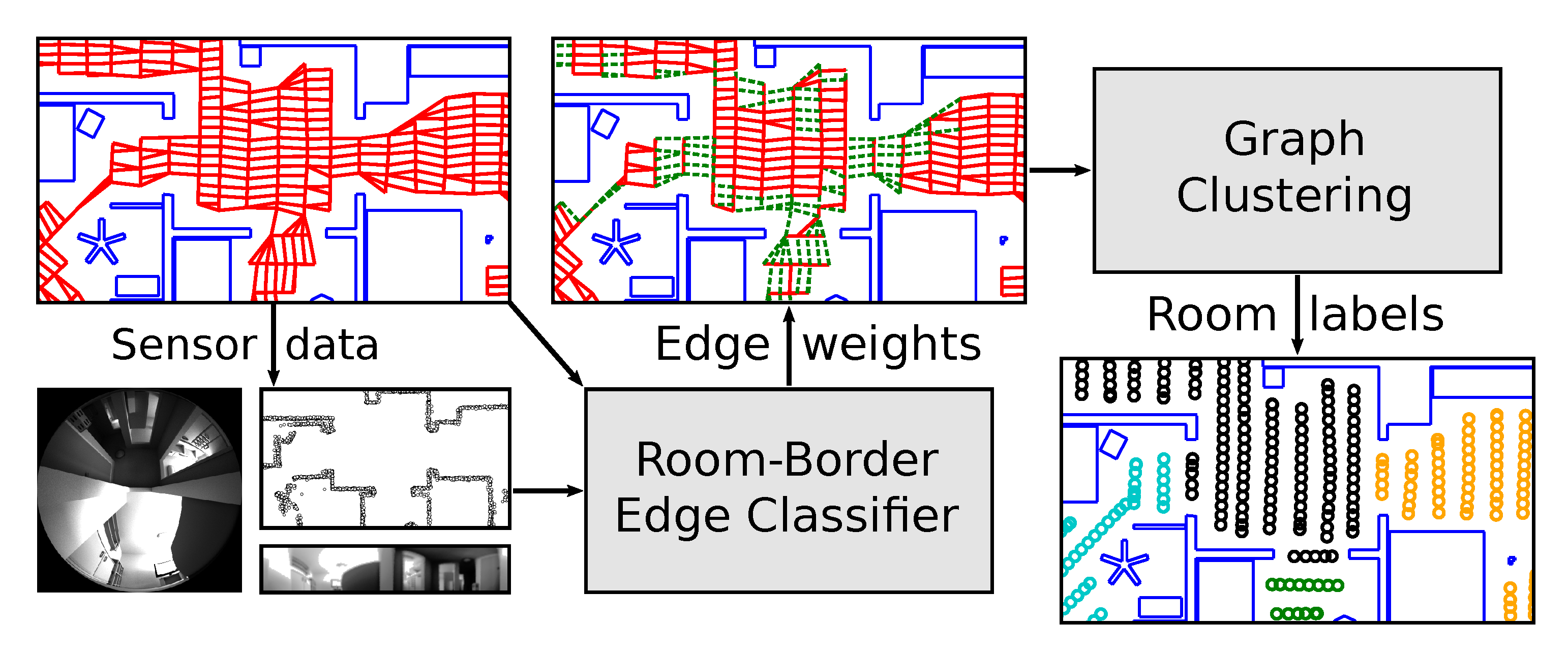
Figure 3.
An example result of our robot’s cleaning strategy. The robot covers the floor space with meandering lanes, shown in red. A circle indicates the beginning of a lane, while an arrowhead indicates its direction. The movement of the robot between the lanes is shown by thin gray lines. The blue lines show the outlines of obstacles, such as walls and furniture. This figure was generated from an experiment in our robot simulator.

Figure 4.
A segment of the robot’s topo-metric map graph, as used for navigation and planning. This map graph was generated from the cleaning run shown in Figure 3. The red lines represent edges in the graph. Each edge connects two nodes, which, for the sake of clarity, are not shown here. As seen in this figure, there are many overlapping edges between the meandering lanes.
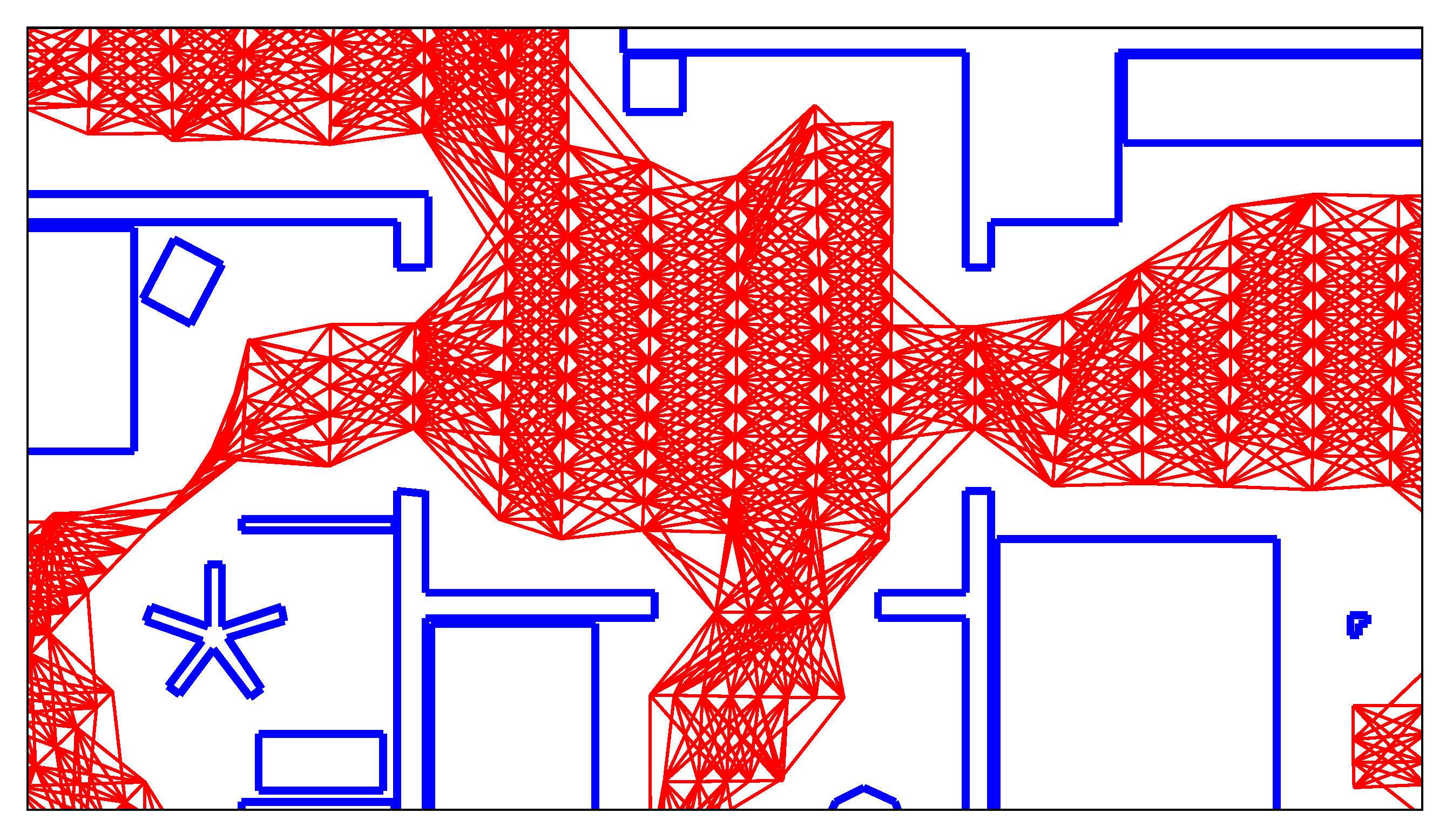
Figure 5.
The map graph from Figure 4, after superfluous edges have been deleted. This kind of comparatively sparse graph is used by all subsequent steps in our method. The black dashed lines show the room borders according to the ground truth.
Figure 5.
The map graph from Figure 4, after superfluous edges have been deleted. This kind of comparatively sparse graph is used by all subsequent steps in our method. The black dashed lines show the room borders according to the ground truth.

Figure 6.
Two examples of the robot’s map graph at a narrow passageway. These figures use the same style as Figure 4. A passageway between two rooms is shown in the center of the image and marked in gray. A hypothetical room border is indicated by a dashed line. Both figures use the same scale, and both passageways are approximately identical in size. However, the room border intersects two edges in (b), compared to five in (a). We compensate for this by adjusting the graph’s edge weights. Note that (a) corresponds to the center-right passageway in Figure 5, rotated clockwise.
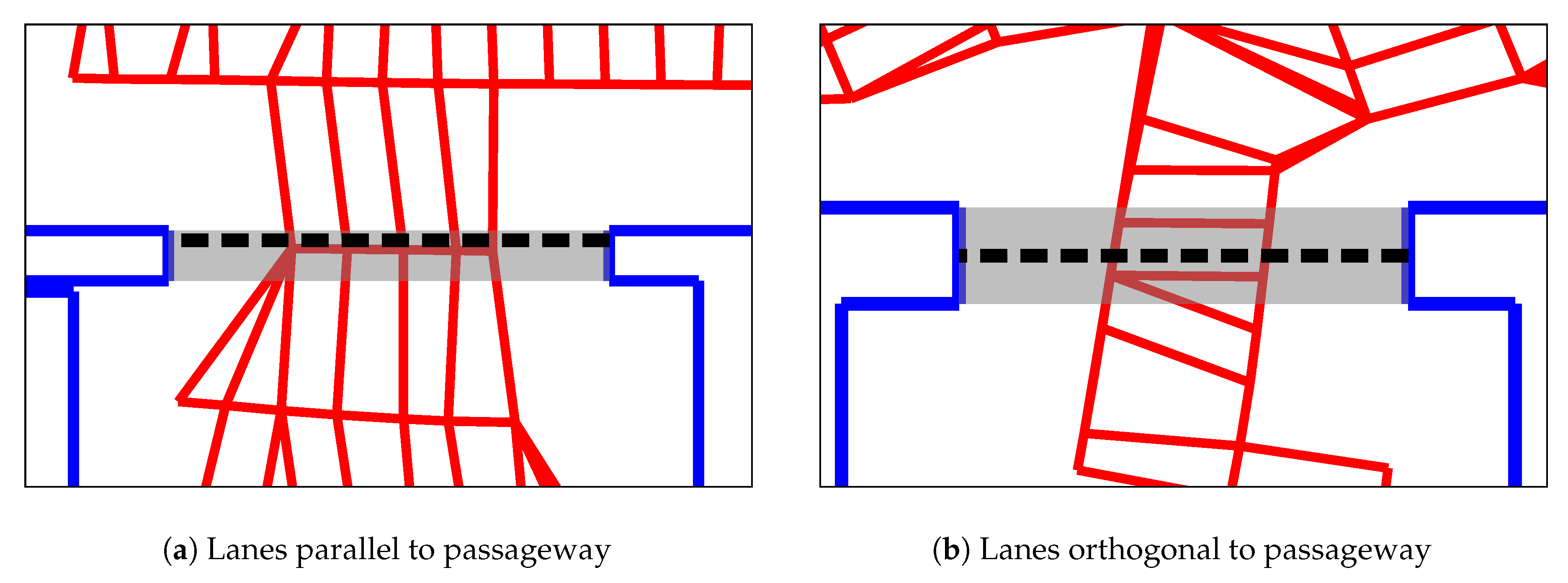
Figure 7.
An illustration of the passageway-width estimation. Obstacle points are shown as black circles. The two blue dots represent to the two nodes in the map graph; they are connected by an edge (blue line) of length l. A pair of dashed gray lines delimit the obstacle search area around the edge. Two red circles correspond to the two obstacle points closest to the edge on each side, as shown by the dotted lines. The distance L (red line) between those two points is the approximate passageway width.

Figure 8.
An illustration of the visual passageway detection heuristic. Passageway detection on the camera image from (a) identifies the edges shown in the detail (b); (b) corresponds to the dashed rectangle in (a). The solid outer ring represents the edge–search cone with an opening angle of . Similarly, the dashed ring corresponds to the edge–offset cone with an angle of . Pixels identified as part of an image edge are highlighted in color. The hue indicates the direction of each pixel’s edge gradient. Next, we construct an edge-pixel histogram from these pixels based on the edge direction and edge offset s. The histogram in (c) shows a clear maximum near the center, corresponding to the lintel. However, this simple heuristic is vulnerable to false positives. In (d), such a false positive is caused by a ceiling lamp.

Figure 9.
We assume a hypothetical passageway to determine the passageway-detection parameters and . Our robot is represented by the small rectangle near the bottom of each figure. The light and dark gray rectangles show the sides and lintel of the passageway, respectively.
Figure 9.
We assume a hypothetical passageway to determine the passageway-detection parameters and . Our robot is represented by the small rectangle near the bottom of each figure. The light and dark gray rectangles show the sides and lintel of the passageway, respectively.
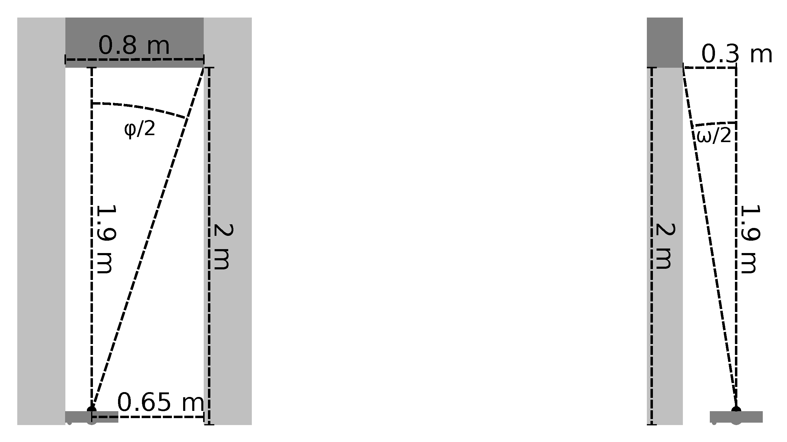
Figure 10.
The geometry of the edge pixels for passageway detection. The position contains an edge pixel with gradient vector and edge–gradient orientation . Mentally extending the edge from gives the dotted black line. If the pixel is part of a straight lintel, the lintel would correspond to this line. The distance between the line and the image center is the edge offset s. The gray circles correspond to the search cones shown in Figure 8b. If lies within the outer search cone, and s is less than the radius of the inner search cone, this pixel will be added to the histogram.

Figure 11.
Receiver Operating Characteristics (ROC) curves for the five edge features used in this work. (a) contains edge features that do not utilize camera images, while (b) contains those that do. For each edge feature, the ROC curve is indicated by a solid line. The location and magnitude of Youden’s J statistic is indicated by a dashed line of the same color. A black, dashed diagonal line indicates the chance level.

Figure 12.
The effect of edge classification on the map graph from Figure 5. Edges classified as crossing a room border are drawn as green, dashed lines. While most room–border edges are classified correctly, we also note some false-positive results within the rooms.
Figure 12.
The effect of edge classification on the map graph from Figure 5. Edges classified as crossing a room border are drawn as green, dashed lines. While most room–border edges are classified correctly, we also note some false-positive results within the rooms.
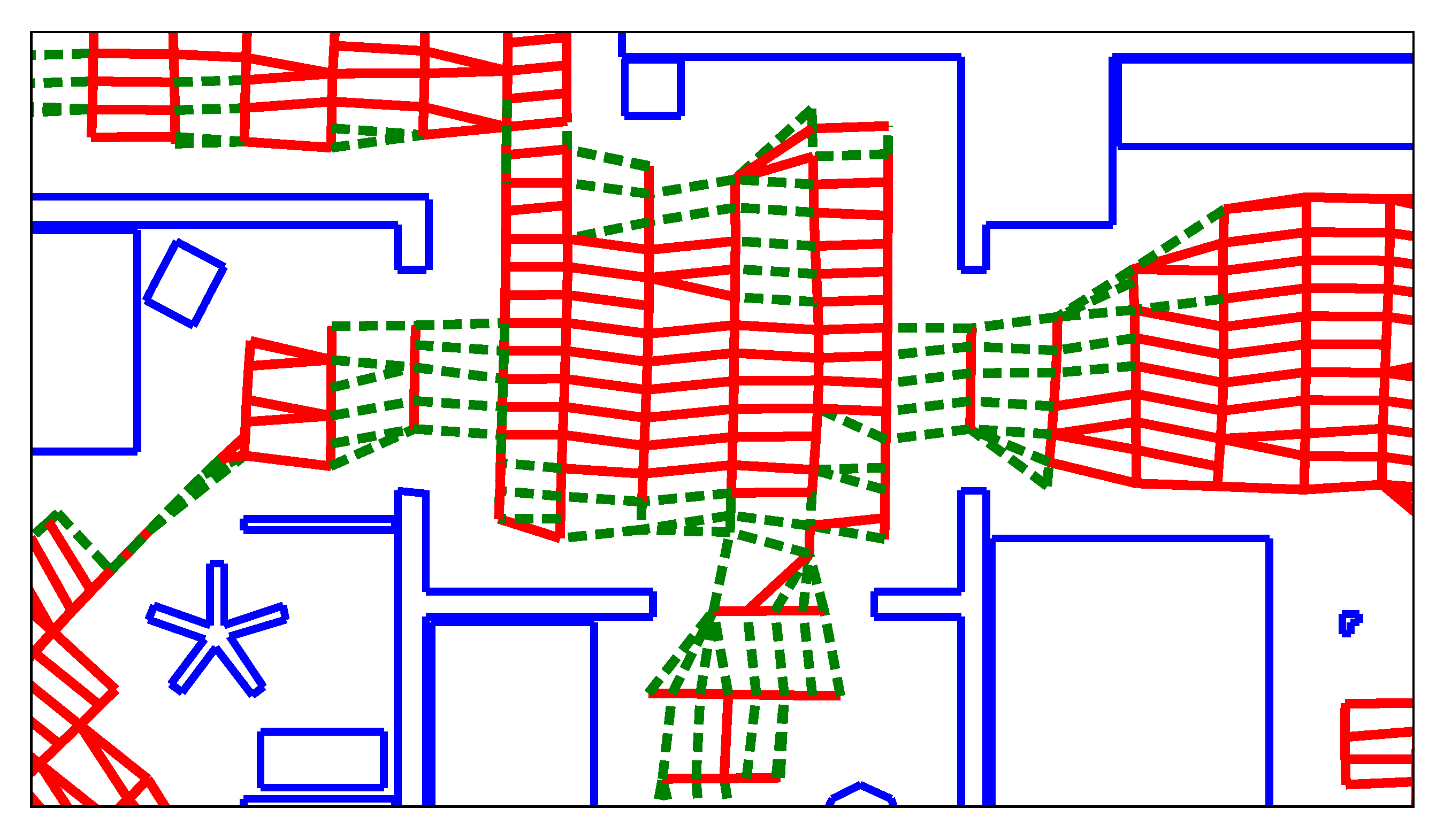
Figure 13.
Plots showing the mean impurity for the full search space listed in Table 4. Values of greater than the maximum of the color scale are shown in dark brown. Only the maps for and are shown here. According to Table 5, these values for w and result in some of the lowest .
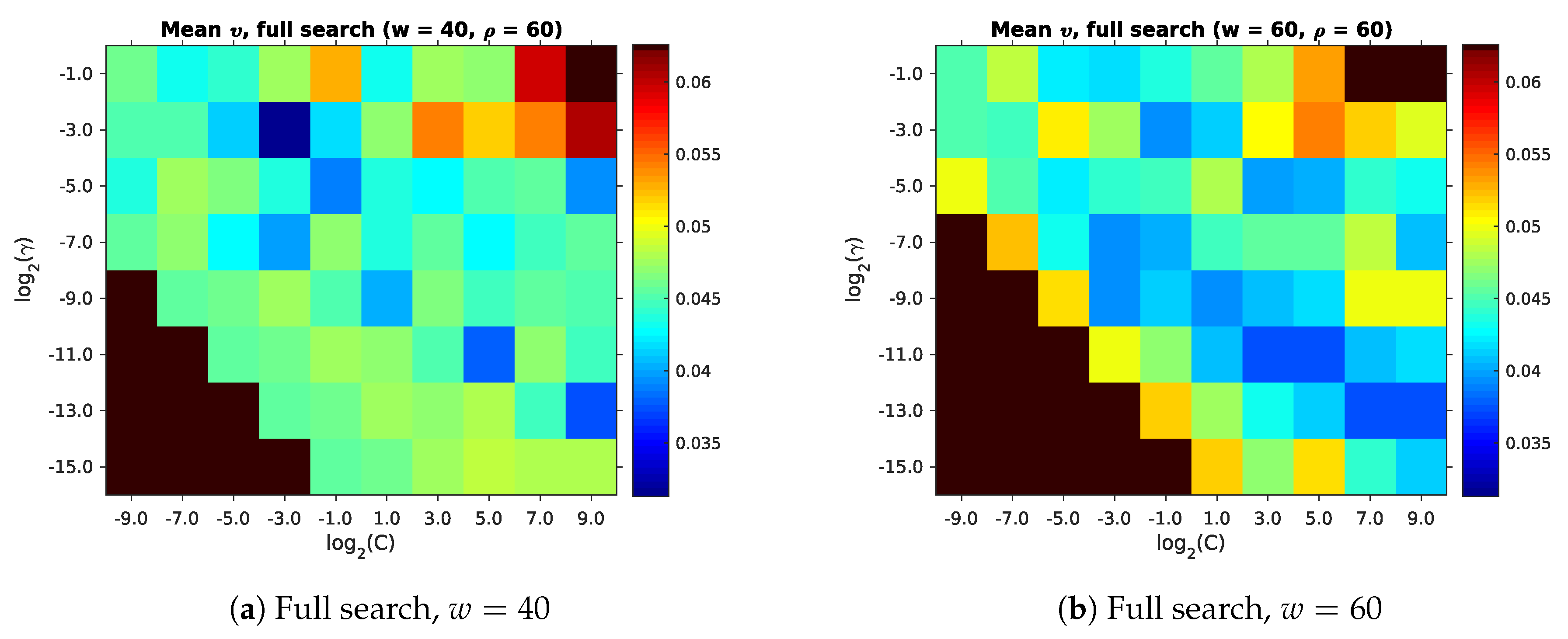
Figure 14.
Plots showing the mean impurity for the fine and extrafine search space listed in Table 4. Values of greater than the maximum of the color scale are shown in dark brown. Only the maps for and are shown, as these contain the lowest according to Table 6.

Figure 15.
The relation between the number of nodes n and room count m. Each mark corresponds to one of our maps. Marks of different color represent different environments.
Figure 15.
The relation between the number of nodes n and room count m. Each mark corresponds to one of our maps. Marks of different color represent different environments.
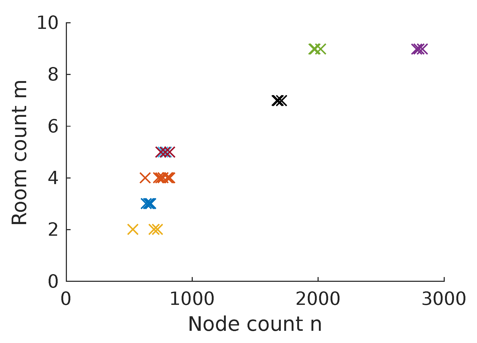
Figure 16.
The three real environments used in this work, according to the obstacle map generated during a cleaning run. Each obstacle point is represented by a small circle. Since our robot’s obstacle map lacks global metric consistency, some walls appear to be slightly curved. Each environment is shown with a checkered bar indicating a length of 5 .
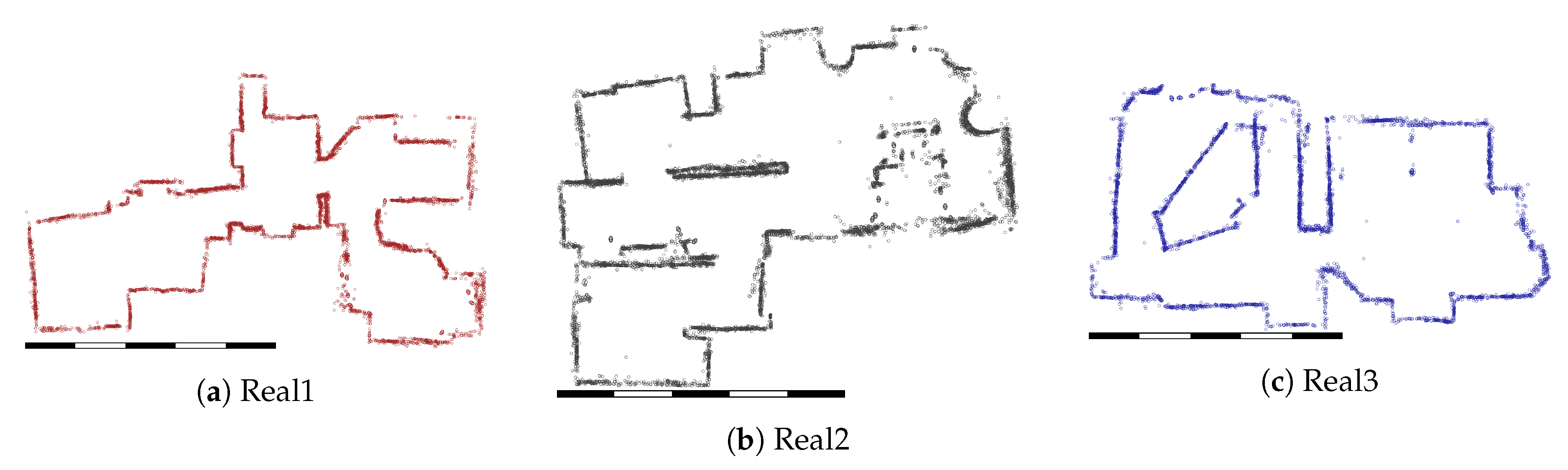
Figure 17.
The unoccupied floor space in each of the five simulated environments. Note that a fraction of the floor space may be inaccessible to the robot due to nearby obstacles. Each environment is shown with a checkered bar indicating a length of 5 .
Figure 17.
The unoccupied floor space in each of the five simulated environments. Note that a fraction of the floor space may be inaccessible to the robot due to nearby obstacles. Each environment is shown with a checkered bar indicating a length of 5 .
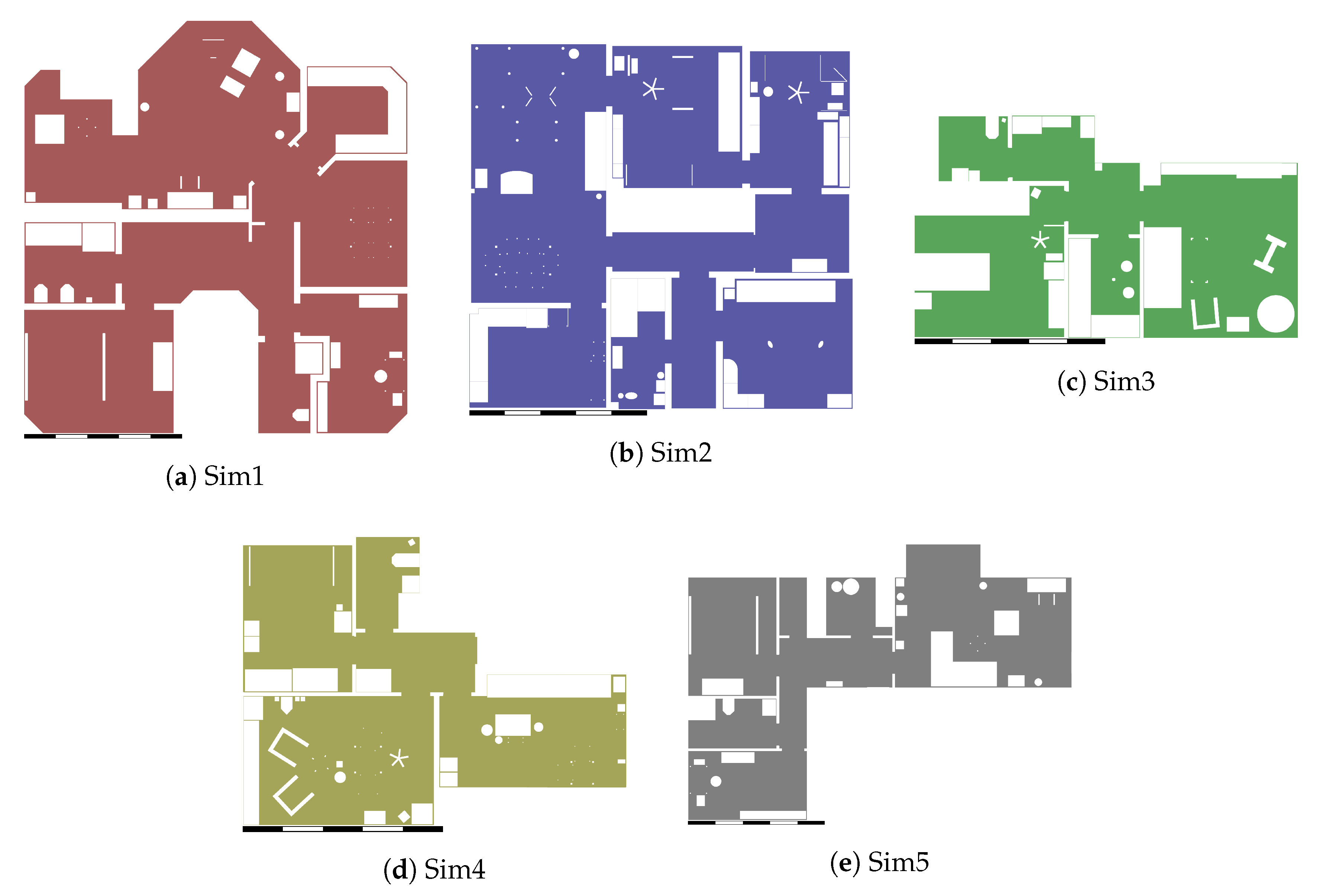
Figure 18.
Panoramic images captured by our robot in three different real environments. The images were captured using a fisheye lens mounted on an upward-facing camera. Only the exposed, inner disc is used by our method.
Figure 18.
Panoramic images captured by our robot in three different real environments. The images were captured using a fisheye lens mounted on an upward-facing camera. Only the exposed, inner disc is used by our method.
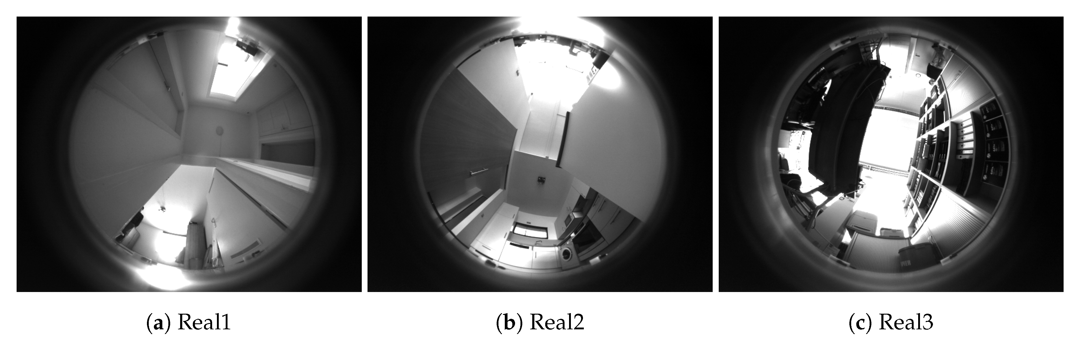
Figure 19.
Low-resolution, unfolded panoramic images acquired by our robot. These images are created by reprojecting, blurring and histogram-equalizing the images in Figure 18. In this work, we use such images to calculate the image distances described in Section 2.2.4. Our robot also performs visual navigation with images of this type.
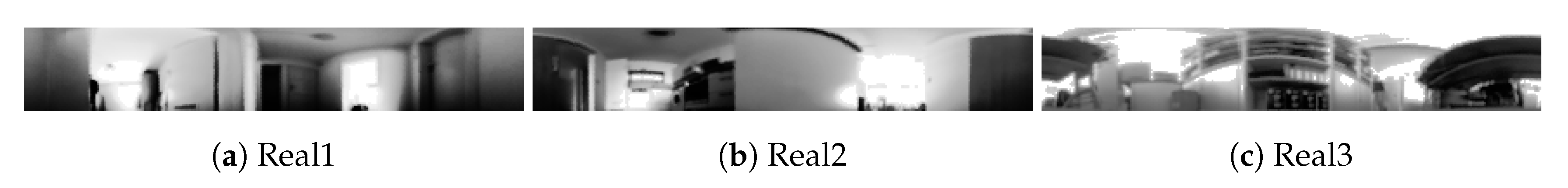
Figure 20.
Rendered camera images, created from the 3D models of our simulated environments. One image is shown for each environment. These images are analogous to the real images shown in Figure 18. The image dimensions are somewhat different from the real camera images. However, the image area and field of view we use within this work are identical.
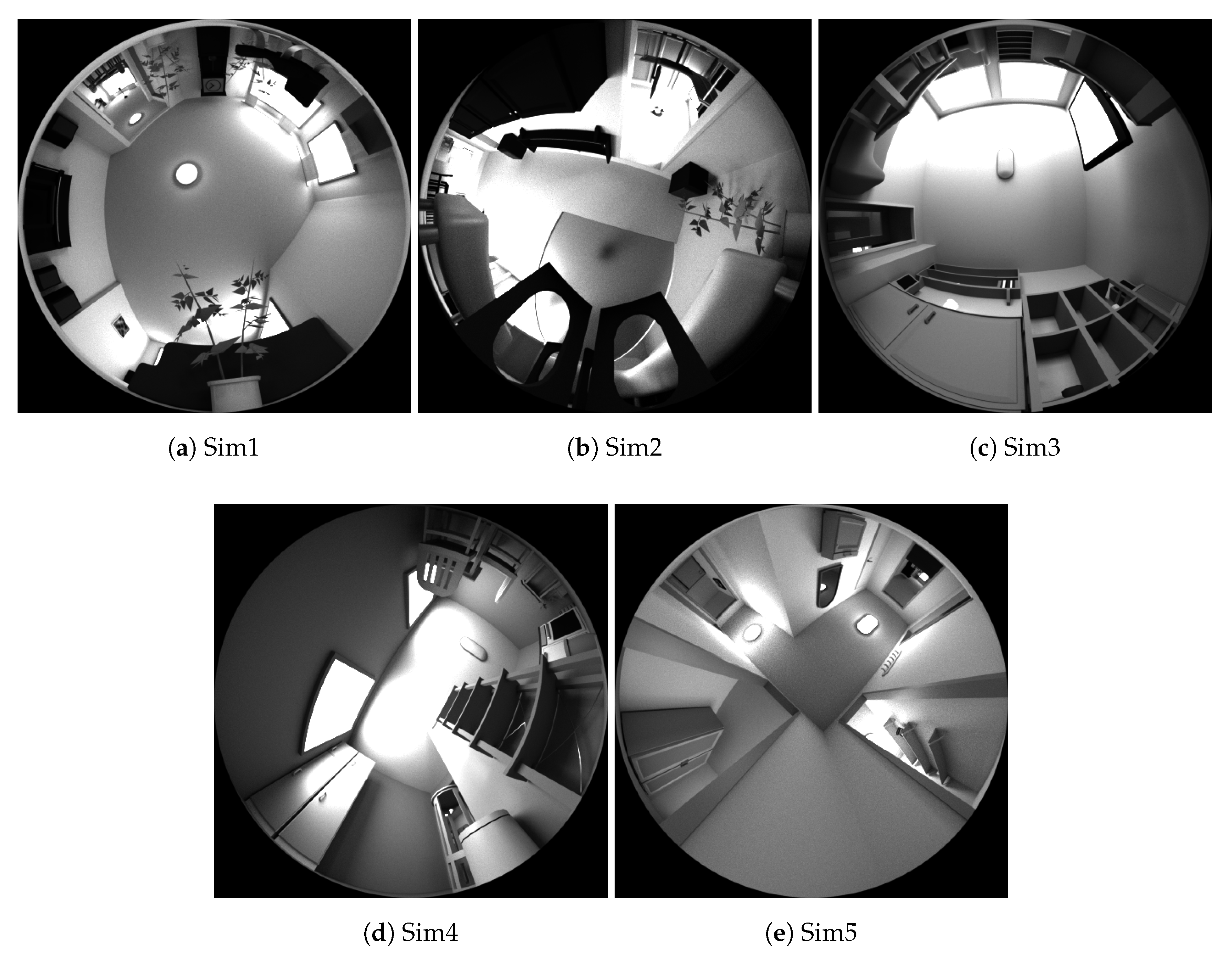
Figure 21.
Unfolded low-resolution images, based on the simulated camera images shown in Figure 20. These images were created in the same manner as those shown in Figure 19.

Figure 22.
An example room segmentation result for the Sim2 simulated environment. (a) shows the ground truth according to Section 3.1.1. Similarly, (b) displays the result of our room segmentation method, using the best parameters from Table 6. Comparing the two sub-figures, we see that our result closely matches the ground truth. Map nodes are represented by circles, and are shown at their true location. Nodes of the same color share the same room label, and therefore belong to the same room. We manually assigned colors to room labels, attempting to associate each color with the same room in both subfigures. Blue lines represent obstacles such as walls or furniture.
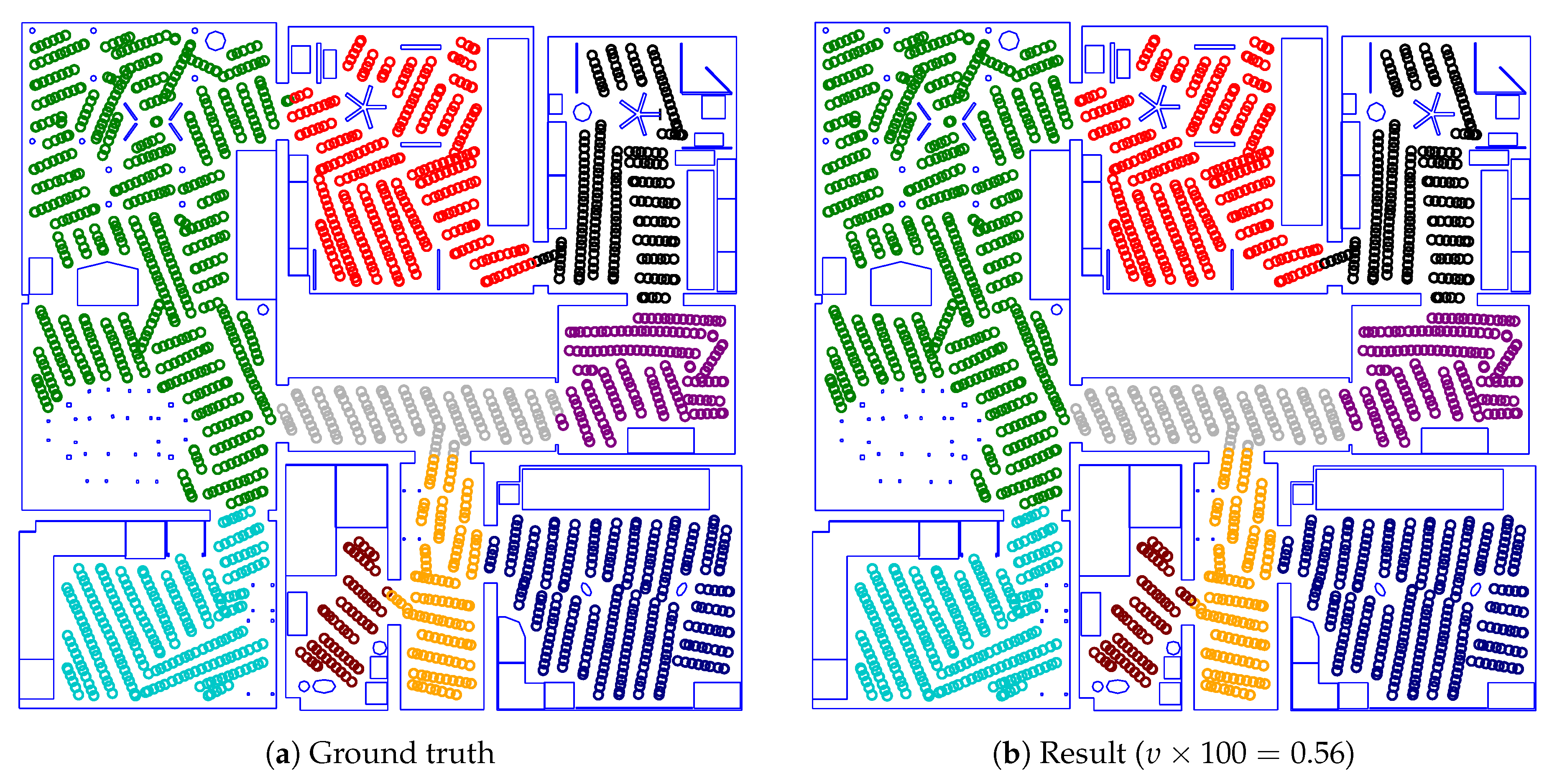
Figure 23.
This figure shows a room segmentation result from the Sim1 environment. Its style is identical to that of Figure 22. In this example, our method failed to correctly segment the small hallway in the upper-right quadrant. As our method uses a fixed room number, the lower-left room is incorrectly split in return.

Figure 24.
A room segmentation example from the Sim4 environment. The style of this plot is described in Figure 22. Here, our method fails to segment the small room near the top. Instead, the larger lower-left room is split at a narrow opening between a wall and a chair.
Figure 24.
A room segmentation example from the Sim4 environment. The style of this plot is described in Figure 22. Here, our method fails to segment the small room near the top. Instead, the larger lower-left room is split at a narrow opening between a wall and a chair.
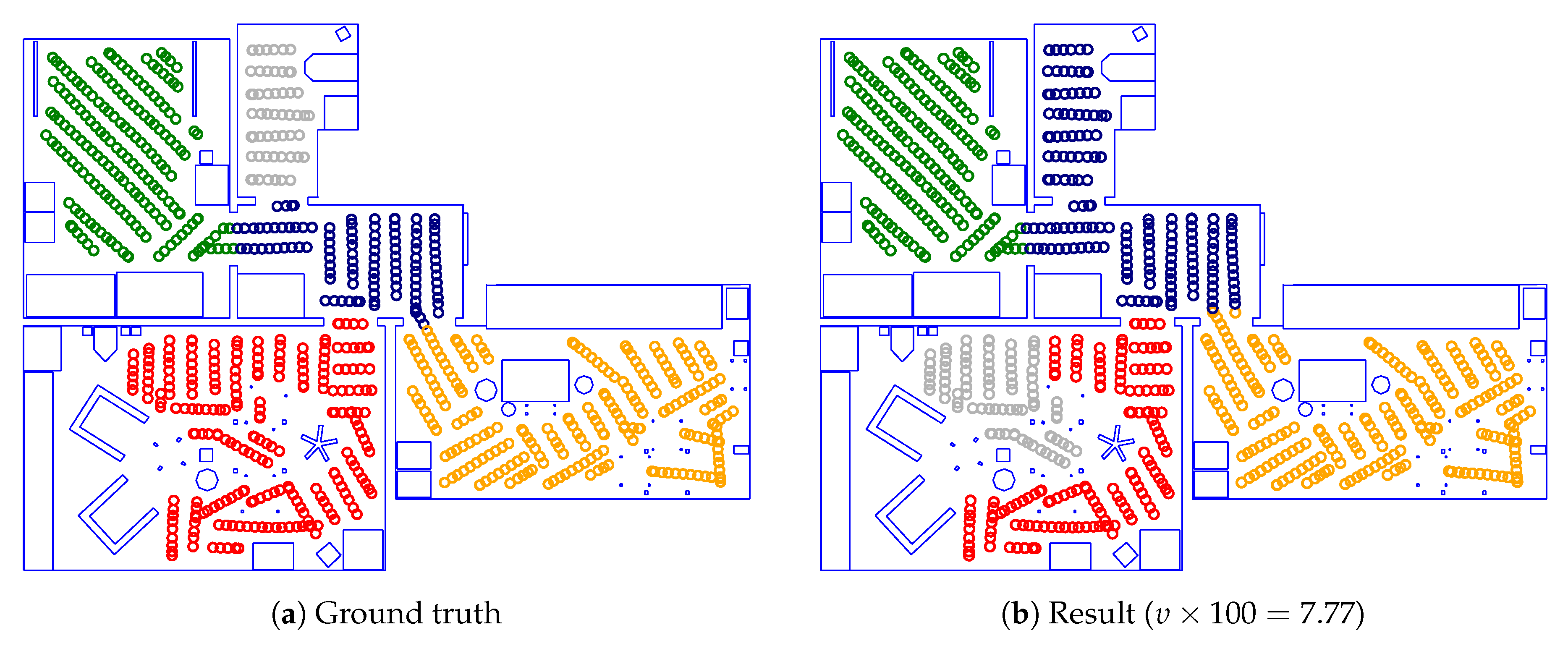
Figure 25.
A room segmentation result for the Real2 environment. This plot is similar to Figure 22, but based on a physical-robot experiment. Therefore, map nodes are plotted according to the robot’s internal position estimate. Small black rings represent points from the robot’s obstacle map. As we will discuss in Section 4.1, most room borders in this environment are relatively indistinct. This causes incorrect room segmentations.
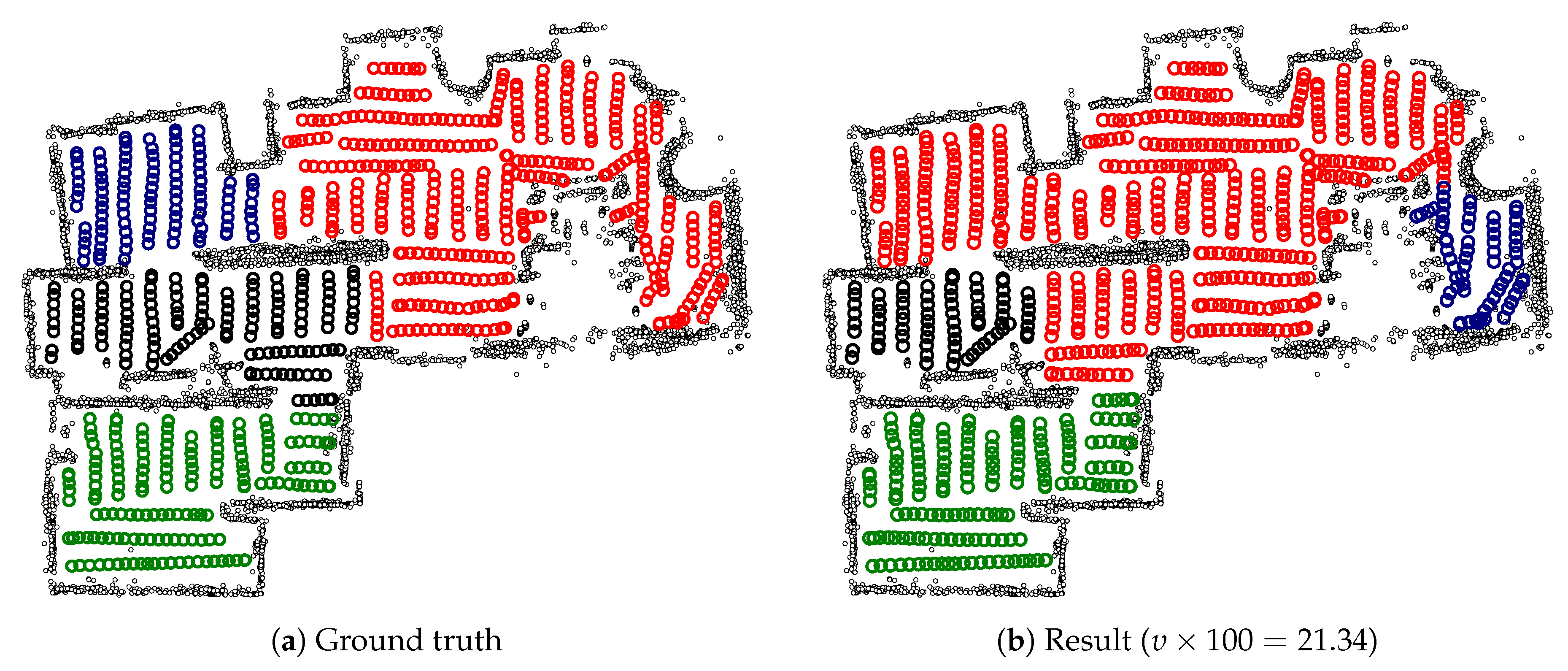
Figure 26.
An overview of the mean impurity for experiments with different edge features. Values are taken from Table 10.
Figure 26.
An overview of the mean impurity for experiments with different edge features. Values are taken from Table 10.
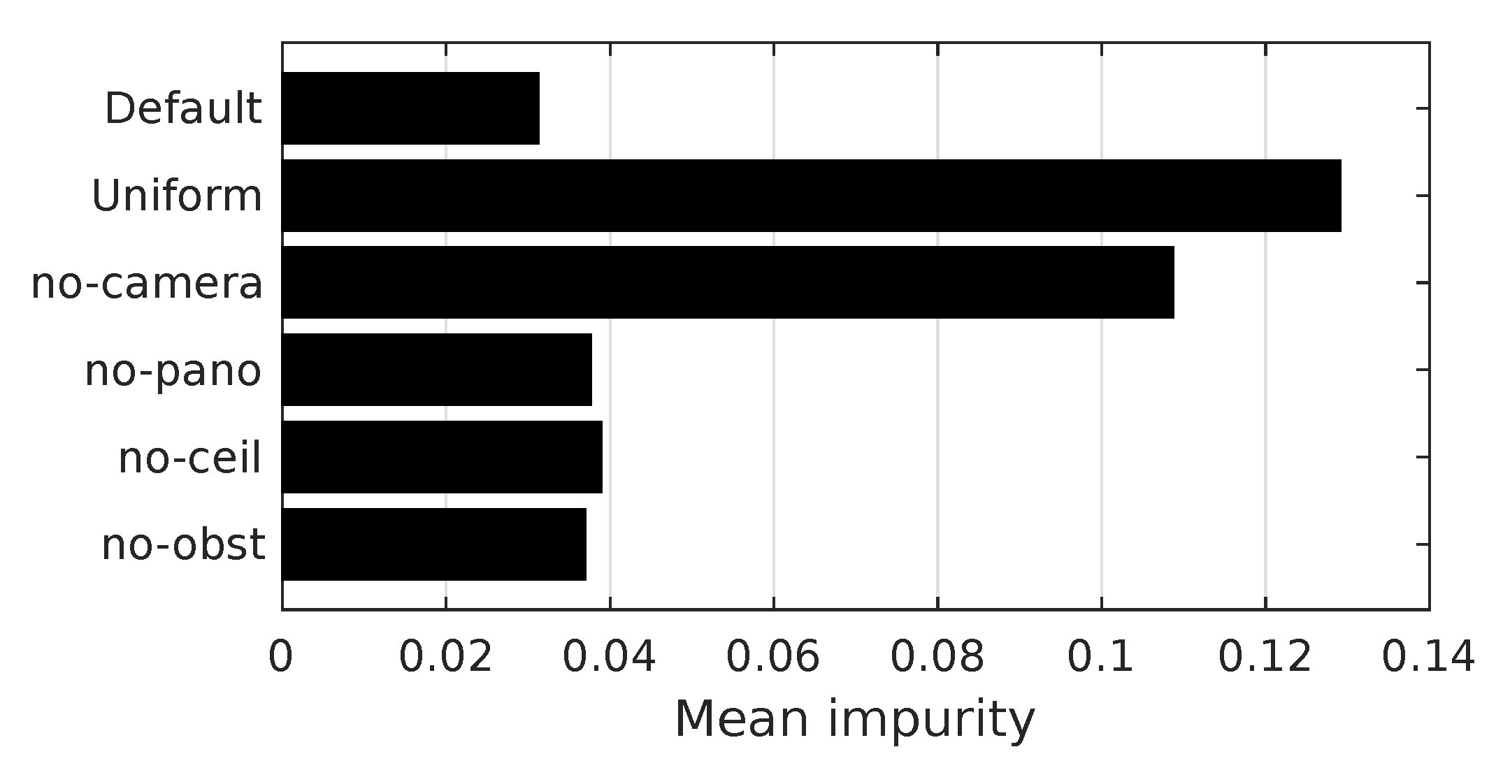
Figure 27.
These plots show results for the Sim5 environment, with and without using the edge classifier. (a) shows the result for our regular method, which is nearly identical to the ground truth (not shown). For (b), we performed room segmentation without adjusting the edge weights. This results in several incorrect room borders. The style of this plot is based on Figure 22.
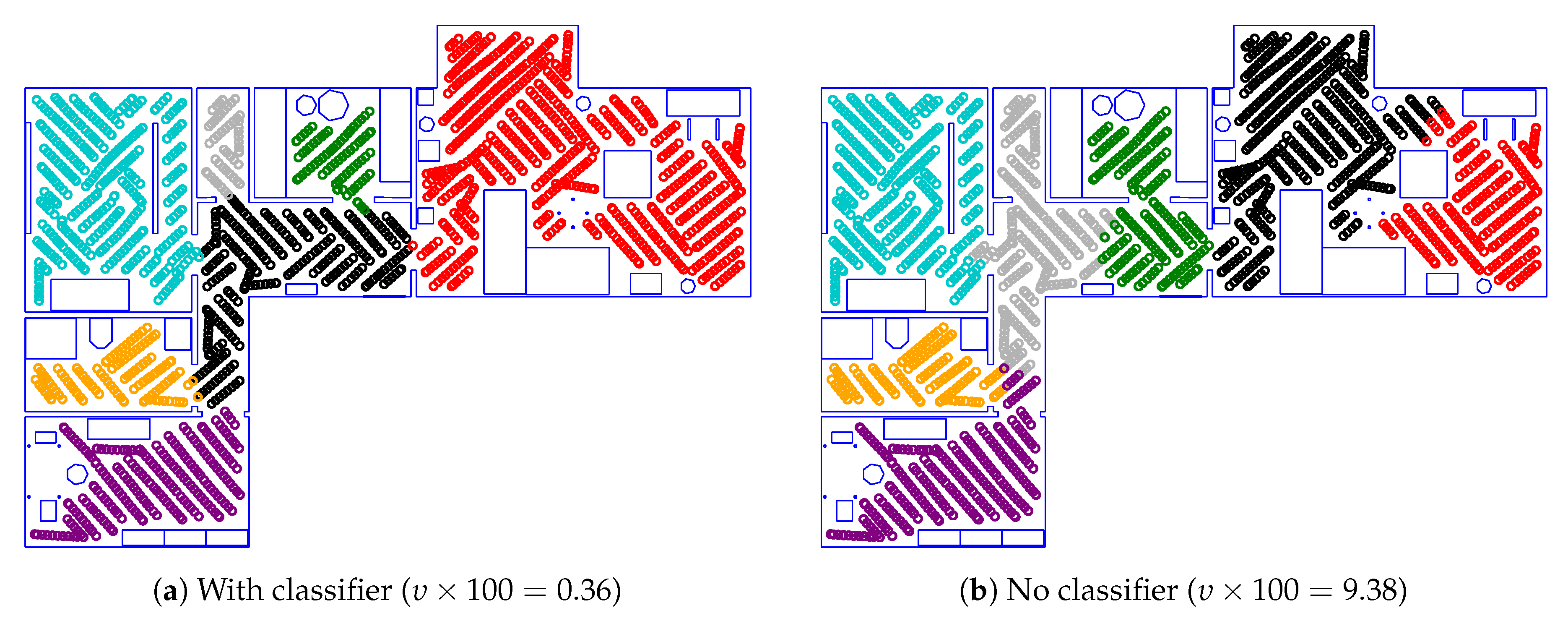
Figure 28.
The unoccupied floor space of the additional test environment, shown in the style of Figure 17. This environment includes a wide passageway connecting the top-left room, very small rooms (top right), and furniture subdividing larger rooms (left).
Figure 28.
The unoccupied floor space of the additional test environment, shown in the style of Figure 17. This environment includes a wide passageway connecting the top-left room, very small rooms (top right), and furniture subdividing larger rooms (left).

Figure 29.
A room segmentation result from the additional simulated environment. The style is identical to that of Figure 22. As seen in (b), our method failed to identify the wide passageway separating the upper-left room. However, all other rooms were segmented correctly.
Figure 29.
A room segmentation result from the additional simulated environment. The style is identical to that of Figure 22. As seen in (b), our method failed to identify the wide passageway separating the upper-left room. However, all other rooms were segmented correctly.
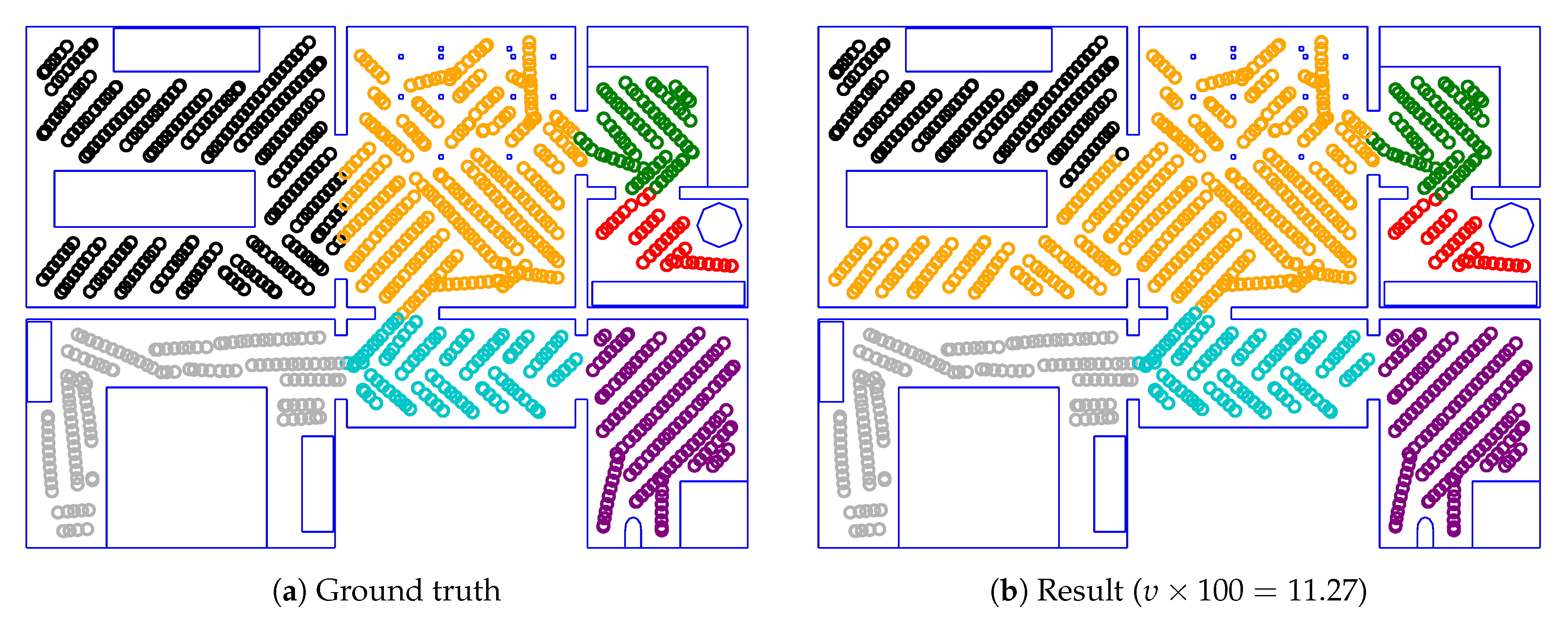
Figure 30.
Our method fails to detect this unusual room border in the Sim1 environment. (a) shows a rendered image of the location. The light red coloration highlights the location of the undetected room border; (b) is a robot-camera image taken at the room border.
Figure 30.
Our method fails to detect this unusual room border in the Sim1 environment. (a) shows a rendered image of the location. The light red coloration highlights the location of the undetected room border; (b) is a robot-camera image taken at the room border.
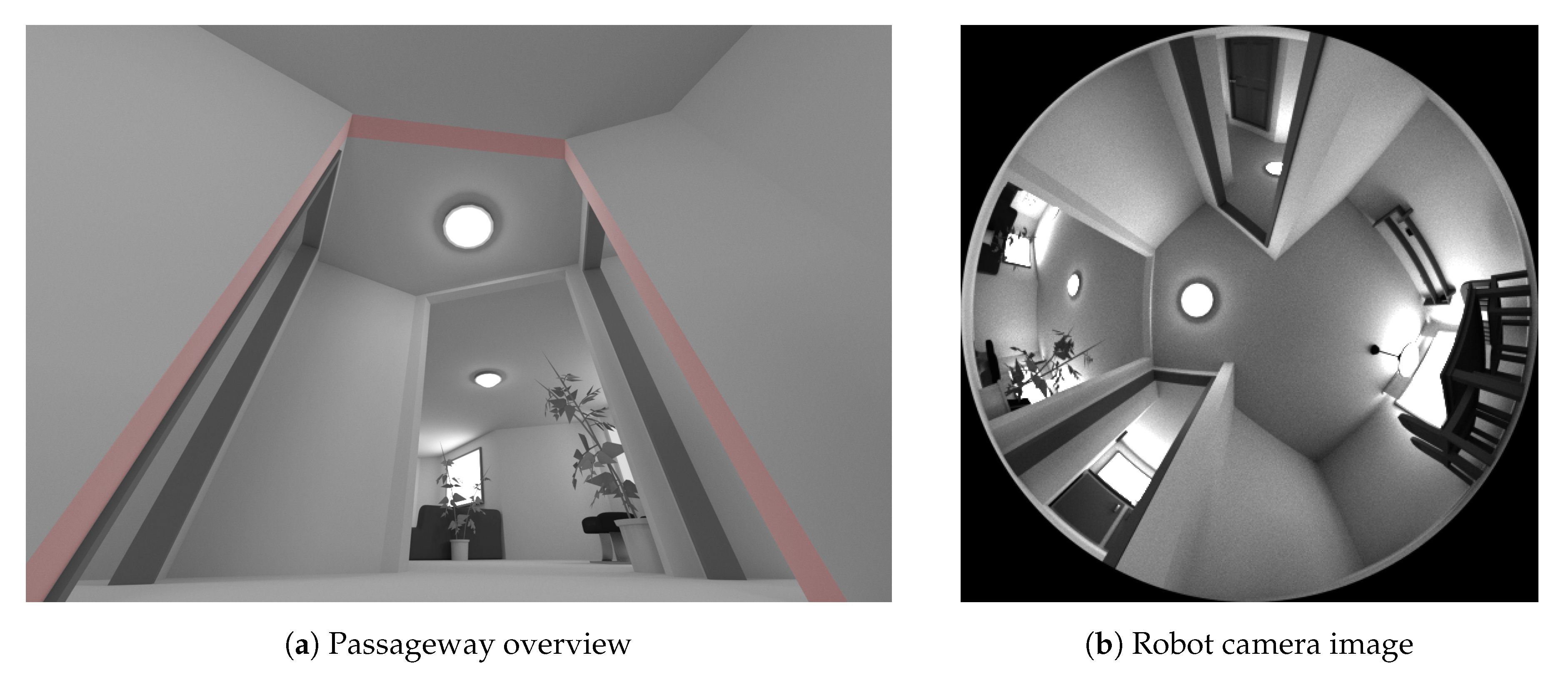
Figure 31.
The Real2 environment also contains unusual room borders. In (a), we highlight two such room borders using color; (b) shows the camera image taken by our robot at the location of the red room–border.
Figure 31.
The Real2 environment also contains unusual room borders. In (a), we highlight two such room borders using color; (b) shows the camera image taken by our robot at the location of the red room–border.
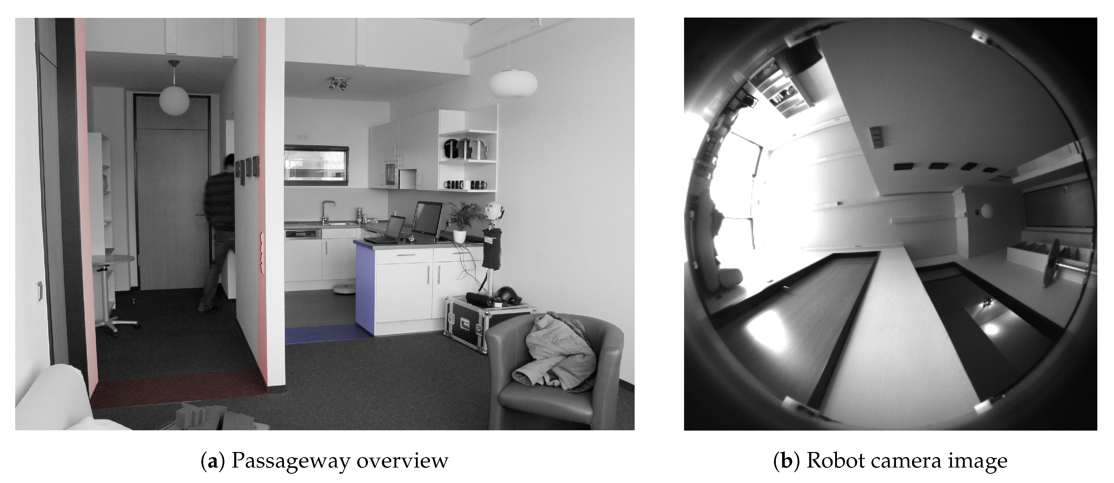

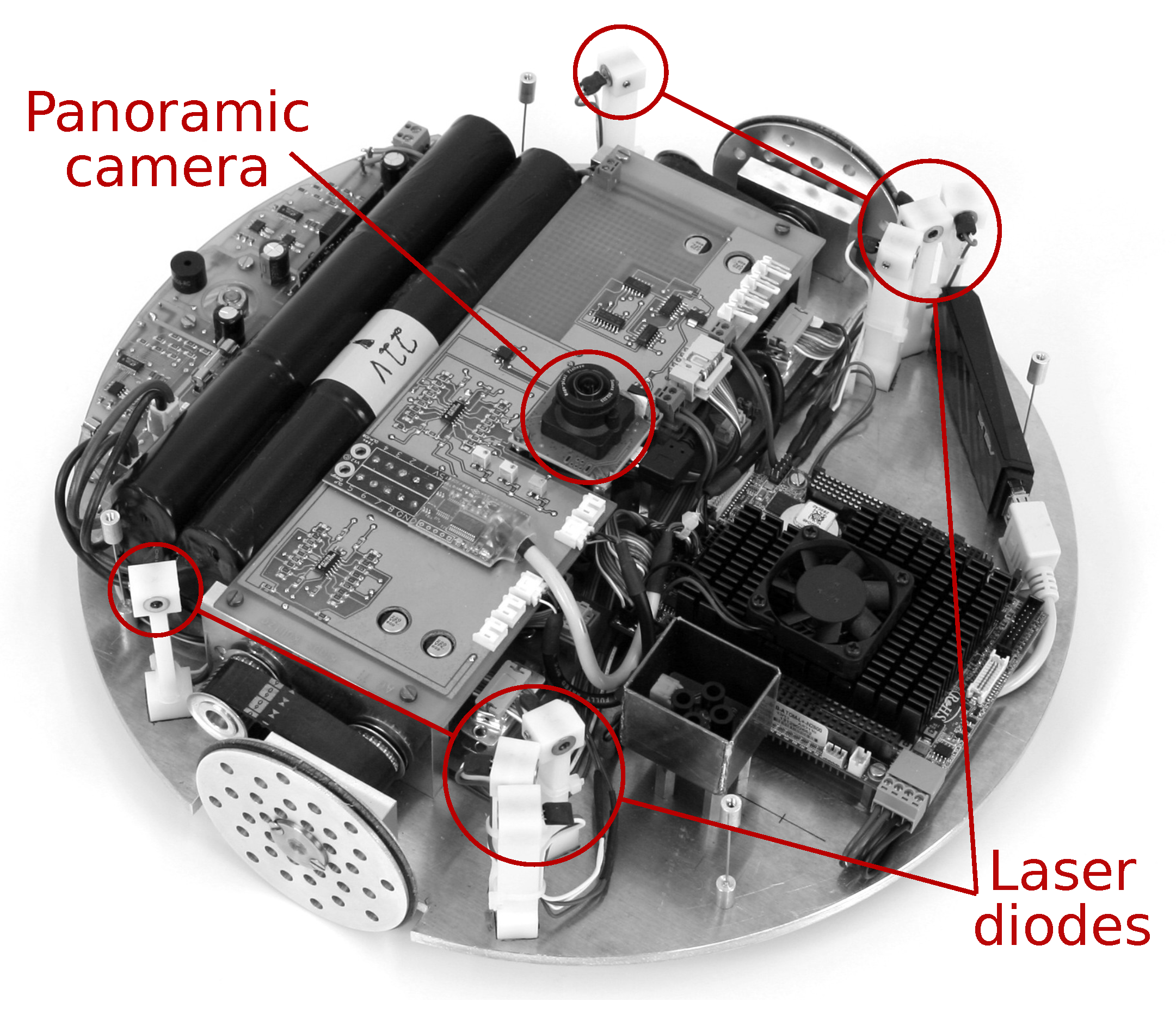
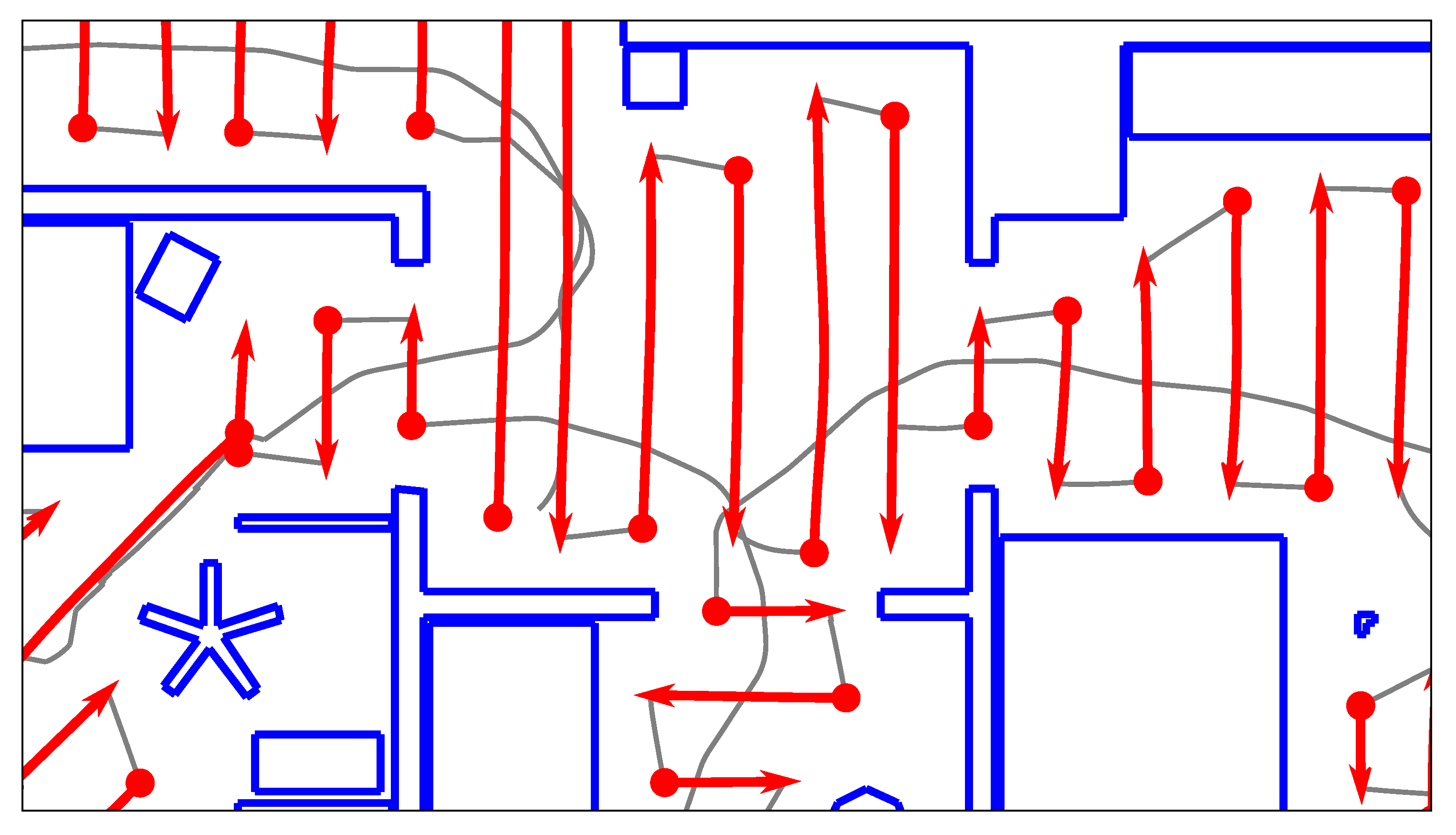
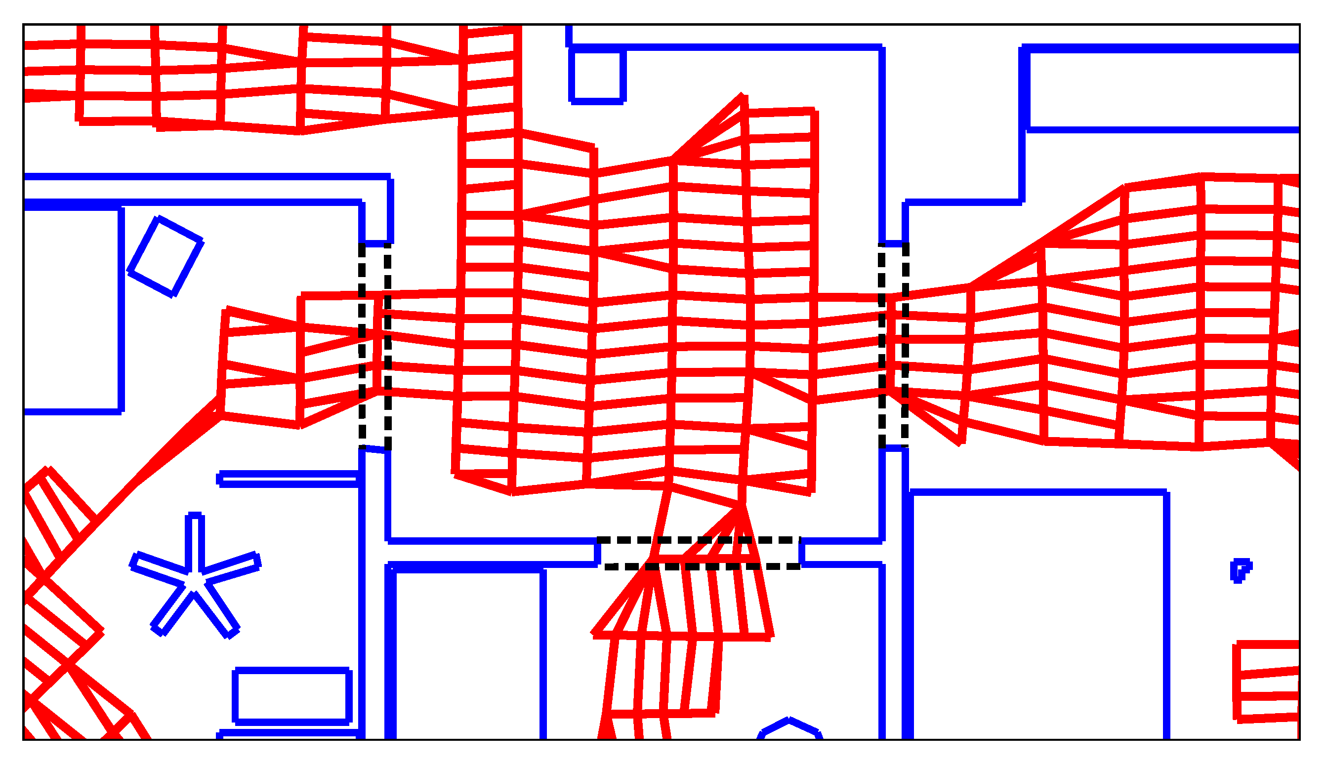
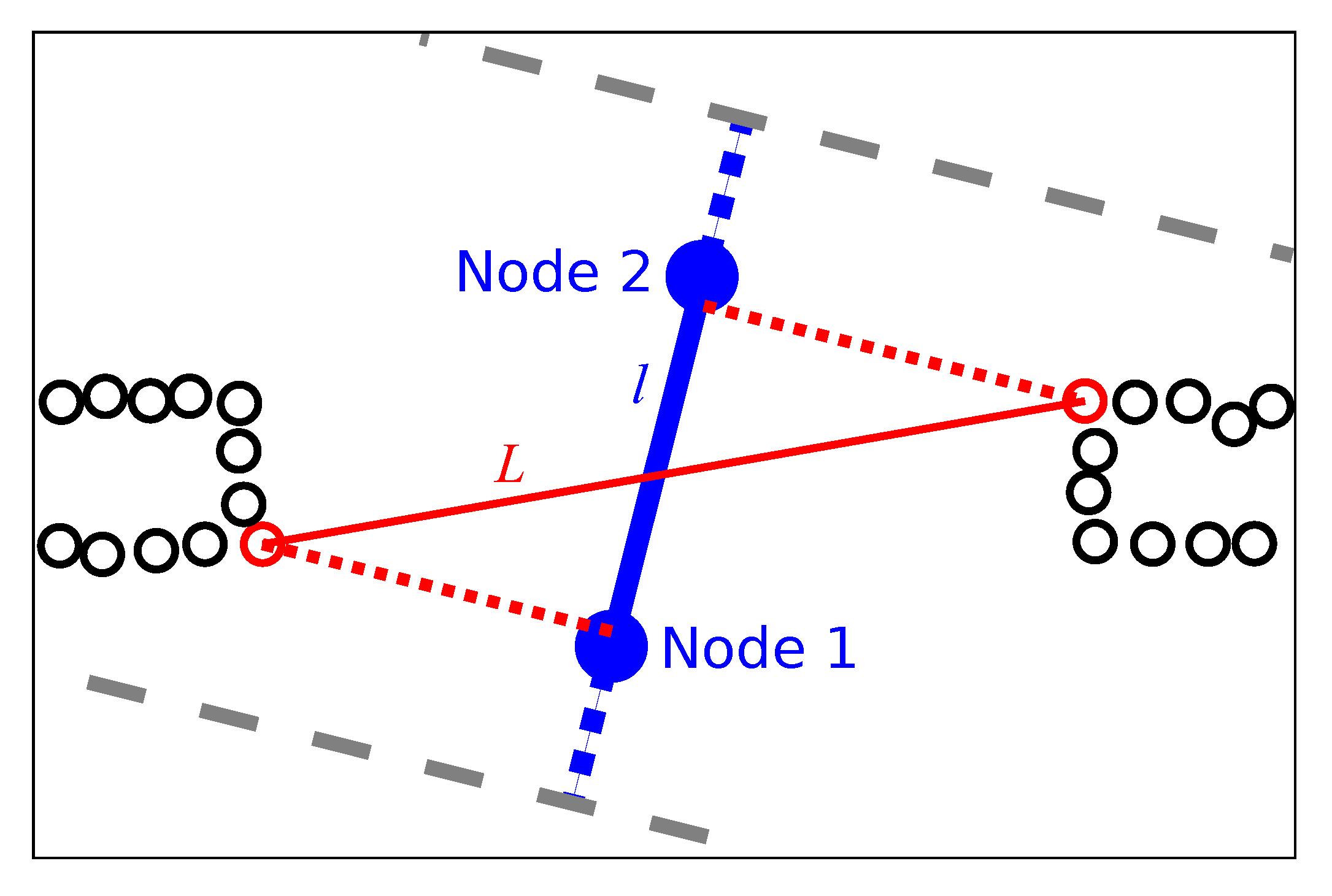
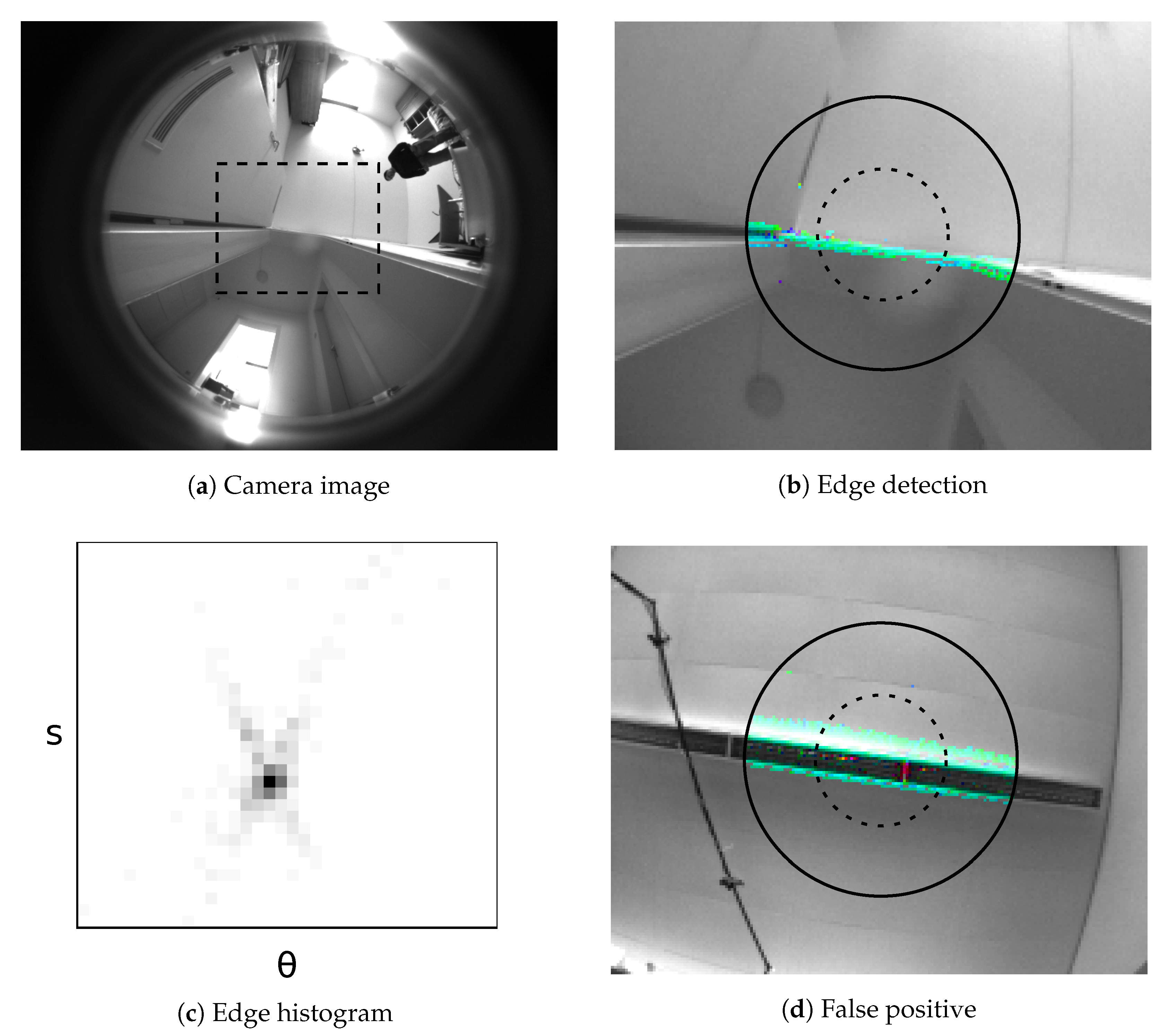
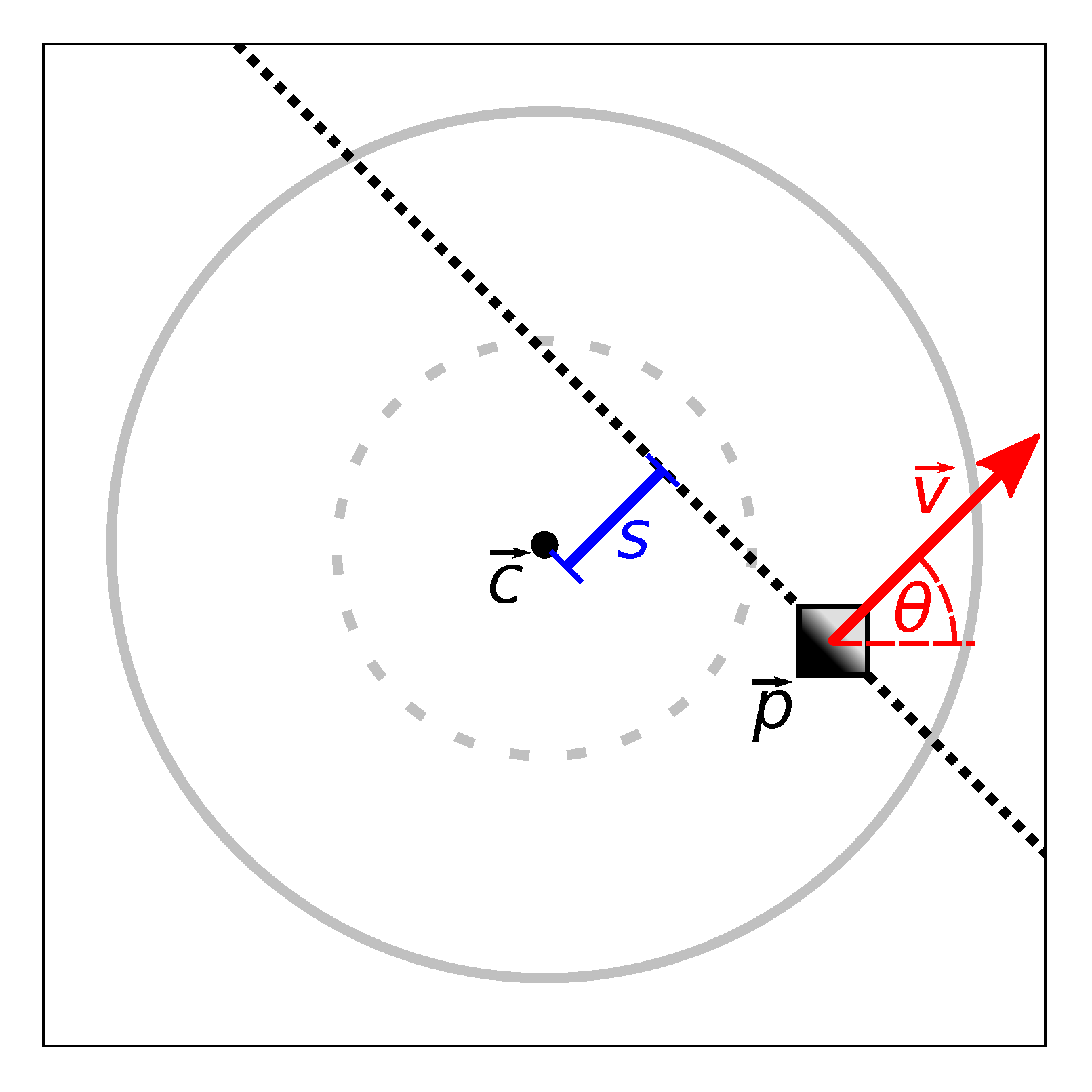
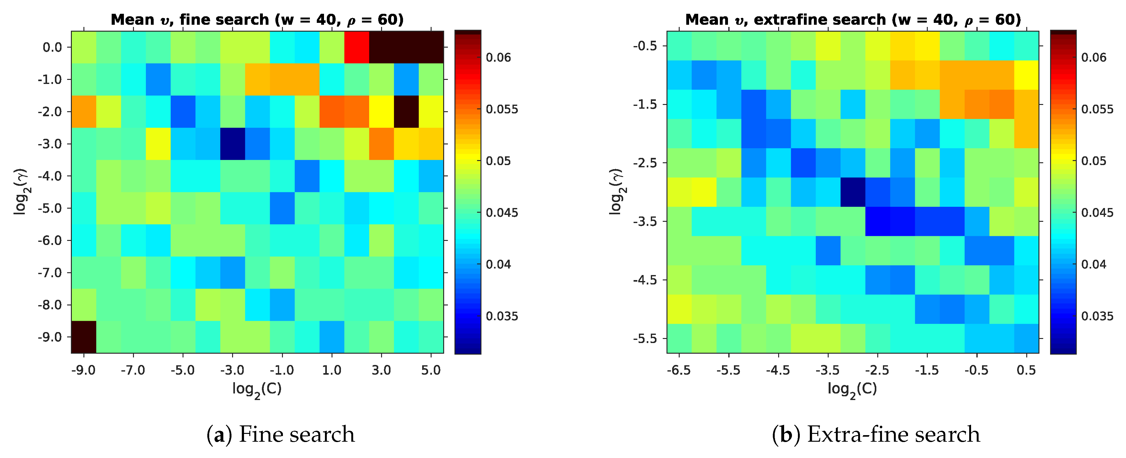
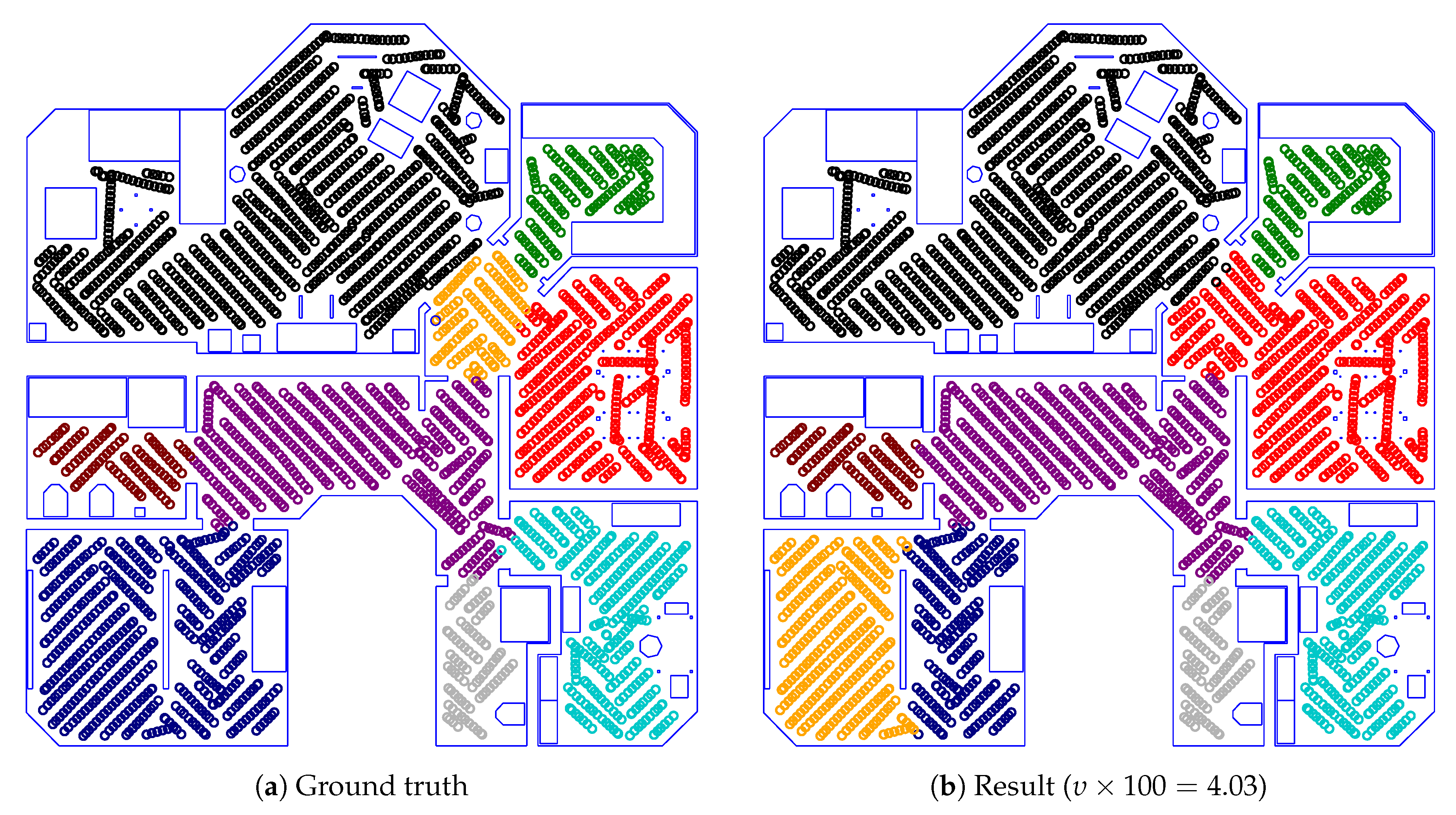
Table 1.
The conditional probability that a random short or long edge crosses a room border. We give these values for short and long edges, which have a length of and respectively. The column labeled gives the overall fraction of short and long edges. Similarly, the row labeled contains the fraction of room–border () and within-room () edges. This table was calculated from the maps described in Section 3.1.
| border | |||
|---|---|---|---|
| 0.008 | 0.992 | 0.498 | |
| 0.043 | 0.957 | 0.502 | |
| 0.026 | 0.974 |
Table 2.
Passageway-detection parameters tested during the search. The parameters with the best area-under-curve are printed in bold, and are used throughout the rest of this work. Note that the bin sizes and are derived from the number of bins and .
Table 2.
Passageway-detection parameters tested during the search. The parameters with the best area-under-curve are printed in bold, and are used throughout the rest of this work. Note that the bin sizes and are derived from the number of bins and .
| Parameter | Values |
|---|---|
| 100, 200, 400 | |
| (18, 17), (36, 33) | |
| 50°, 55°, 60°, 65°, 70°, 80°, 90° |
Table 3.
The area-under-curve and Youden’s J statistic for each of the five edge features. When used as a heuristic for edge-feature selection, high values should indicate a useful feature.
Table 3.
The area-under-curve and Youden’s J statistic for each of the five edge features. When used as a heuristic for edge-feature selection, high values should indicate a useful feature.
| Edge Feature | Area under Curve | J |
|---|---|---|
| Edge length | 0.71 | 0.35 |
| Obstacle data | 0.78 | 0.56 |
| Passageway detection | 0.87 | 0.61 |
| Image distance | 0.77 | 0.40 |
| Image distance | 0.66 | 0.29 |
Table 4.
Parameter search spaces used for our room segmentation method. For each search, all possible values of C, , w and are combined, resulting in a total of p parameter combinations. Here, , for example .
Table 4.
Parameter search spaces used for our room segmentation method. For each search, all possible values of C, , w and are combined, resulting in a total of p parameter combinations. Here, , for example .
| Experiment | w | p | |||
|---|---|---|---|---|---|
| full | −9:2:9 | −15:2:−1 | 20, 40, 60 | 20:20:120 | 1440 |
| fine | −9:1:5 | −9:1:0 | 40 | 50:10:80 | 600 |
| extrafine | −6.5:0.5:0.5 | −5.5:0.5:−0.5 | 40 | 50, 60, 70 | 495 |
Table 5.
The results of the parameter search over the full search space specified in Table 4. We sort results according to the lowest mean impurity over all environments, and list only the first ten entries. The parameters with the lowest impurity are given in bold, and are used in most of our subsequent experiments. This table also contains the median impurity . For the sake of readability, the impurities have been multiplied by a factor of 100.
| w | |||||
|---|---|---|---|---|---|
| −3 | −3 | 40 | 60 | 3.13 | 1.04 |
| −3 | −3 | 40 | 80 | 3.15 | 1.12 |
| −3 | −3 | 40 | 100 | 3.55 | 1.12 |
| −3 | −3 | 40 | 120 | 3.55 | 1.12 |
| 3 | −11 | 60 | 60 | 3.72 | 1.30 |
| 9 | −13 | 60 | 60 | 3.73 | 1.37 |
| 7 | −13 | 60 | 60 | 3.74 | 1.30 |
| 5 | −11 | 60 | 60 | 3.74 | 1.37 |
| 9 | −13 | 40 | 60 | 3.75 | 1.63 |
| 9 | −13 | 40 | 80 | 3.76 | 1.63 |
Table 6.
The results of the parameter search over the extrafine search space specified in Table 4. Results are sorted according to the lowest mean impurity , and only the first five entries are shown here. The result with the lowest is printed in bold. All other details are as in Table 5.
| w | |||||
|---|---|---|---|---|---|
| −3.0 | −3.0 | 40 | 60 | 3.13 | 1.04 |
| −3.0 | −3.0 | 40 | 70 | 3.13 | 1.04 |
| −3.0 | −3.0 | 40 | 50 | 3.19 | 1.37 |
| −2.0 | −3.5 | 40 | 50 | 3.35 | 1.65 |
| −2.5 | −3.5 | 40 | 60 | 3.50 | 1.04 |
Table 7.
This table describes the room count estimation results. is the average absolute room count estimation error over all maps. The fraction of maps for which each method gives the correct result is . Similarly, the fraction for which the error is at most one is given as .
Table 7.
This table describes the room count estimation results. is the average absolute room count estimation error over all maps. The fraction of maps for which each method gives the correct result is . Similarly, the fraction for which the error is at most one is given as .
| Method | |||
|---|---|---|---|
| Map-node regression | 0.68 | 0.42 | 0.90 |
| Eigenvalue gap | 0.77 | 0.45 | 0.81 |
Table 8.
The properties of our test and training environments. The second column lists the number of different maps included in the training set. The Area is the total floor-space, as calculated from the 3D model. This includes space that is covered by furniture, or otherwise inaccessible to the robot. Unfortunately, this value is not available for the real environments. We also list the average number of Map nodes; this is approximately proportional to the area covered while cleaning. The Rooms column gives nominal room count derived from the ground truth. The Passageway contrast describes the visual distinctiveness of the majority of room–border passageways. This qualitative judgment is based on a visual inspection of the camera images. High-contrast passageways are visually distinct relative to the surrounding walls and ceiling. Conversely, a low-contrast passageway may appear similar to the surrounding structure. Finally, the Lighting attribute indicates whether an environment is lit more by interior or exterior light sources.
| Name | # | Area [m] | Map Nodes | Rooms | Passageway Contrast | Lighting |
|---|---|---|---|---|---|---|
| Sim1 | 3 | 125 | 2806 | 9 | High | Interior |
| Sim2 | 3 | 101 | 1988 | 9 | Low | Mixed |
| Sim3 | 3 | 51 | 787 | 5 | Low | Exterior |
| Sim4 | 3 | 46 | 783 | 5 | Medium | Exterior |
| Sim5 | 3 | 79 | 1688 | 7 | High | Interior |
| Real1 | 5 | - | 656 | 3 | Low | Exterior |
| Real2 | 8 | - | 760 | 4 | Low | Exterior |
| Real3 | 3 | - | 649 | 2 | High | Exterior |
Table 9.
Parameter search spaces for experiments with partial edge features, using the notation from Table 4. All no-* experiments also include the basic search space. For these experiments, n includes only parameter combinations not already part of the basic search space.
Table 9.
Parameter search spaces for experiments with partial edge features, using the notation from Table 4. All no-* experiments also include the basic search space. For these experiments, n includes only parameter combinations not already part of the basic search space.
| Experiment | w | p | |||
|---|---|---|---|---|---|
| basic | −9:2:9 | −15:2:−1 | 40 | 20:20:120 | 480 |
| no-camera | −9:2:11 | −15:2:1 | 40 | 2.5, 5, 10, 20 | 316 |
| no-pano | same as basic | 0 | |||
| no-ceiling | −9:2:15 | −19:2:−1 | 40 | 20:20:120 | 300 |
| no-obst | same as basic | 0 | |||
Table 10.
The results of the experiments with partial edge features. For each variant, we give the parameters with the lowest mean impurity . We also include the median impurities . Default refers to the results achieved with all edge features, as in Table 5. For the uniform results, we did not use an edge classifier. Instead, all edges in the map graph had a uniform weight of 1. For this reason, the corresponding row also contains no parameters.
| w | ||||||
|---|---|---|---|---|---|---|
| Default | −3 | −3 | 40 | 60 | 3.13 | 1.04 |
| uniform | - | - | - | - | 12.91 | 15.46 |
| no-camera | −1 | −3 | 40 | 5 | 10.87 | 9.67 |
| no-pano | 5 | −13 | 40 | 100 | 3.76 | 1.07 |
| no-ceiling | 15 | −13 | 40 | 60 | 3.89 | 1.37 |
| no-obst | −5 | −3 | 40 | 80 | 3.69 | 1.21 |
© 2017 by the author. Licensee MDPI, Basel, Switzerland. This article is an open access article distributed under the terms and conditions of the Creative Commons Attribution (CC BY) license (http://creativecommons.org/licenses/by/4.0/).
Share and Cite
MDPI and ACS Style
Fleer, D. Human-Like Room Segmentation for Domestic Cleaning Robots. Robotics 2017, 6, 35. https://doi.org/10.3390/robotics6040035
AMA Style
Fleer D. Human-Like Room Segmentation for Domestic Cleaning Robots. Robotics. 2017; 6(4):35. https://doi.org/10.3390/robotics6040035
Chicago/Turabian StyleFleer, David. 2017. "Human-Like Room Segmentation for Domestic Cleaning Robots" Robotics 6, no. 4: 35. https://doi.org/10.3390/robotics6040035
Note that from the first issue of 2016, this journal uses article numbers instead of page numbers. See further details here.