A Simple Robotic Eye-In-Hand Camera Positioning and Alignment Control Method Based on Parallelogram Features

Abstract

A simple and effective method for camera positioning and alignment control for robotic pick-and-place tasks is described here. A parallelogram feature is encoded into each 3D object or target location. To determine the pose of each part and guide the robot precisely, a camera is mounted on the robot end-flange to determine and measure the location and pose of the part. The robot then adjusts the camera to align it with the located part so that it can be grasped. The overall robot control system follows a continuous look-and-move control strategy. After a position-based coarse alignment, a sequence of image-based fine alignment steps is carried out, and the part is then picked and placed by the robot arm gripper. Experimental results showed an excellent applicability of the proposed approach for pick-and-place tasks, and the overall errors were 1.2 mm for positioning and 1.0° for orientation angle.

1. Introduction

There is an abundance of different literature on vision-based robot control. In this technology, image information is used to measure the error between the current position and orientation (pose) of a robot and its desired reference pose [1,2]. A position-based visual servo (PBVS) system estimates the three-dimensional measurements of the target’s pose with respect to a camera Cartesian coordinate frame [3], while an image-based visual servo (IBVS) system estimates two-dimensional measurements in image plane coordinates and directs the desired movement of the robot. A hybrid visual servo uses a combination of PBVS and IBVS, in which some errors are specified in the image pixel space and some in the Cartesian pose space.

A vision-guide robot control system may use visual information in two different ways: open-loop robot control and closed-loop visual feedback control. In the open-loop approach, the robot movement is based on the visual information extracted in the Cartesian frame; thus, the camera has to be calibrated with respect to the robot. However, camera calibration is known to be an error prone process. Perfect calibration of the robot/camera system is difficult, time-consuming, and sometimes even impossible to achieve.

There are two ways to implement vision-feedback robot control: the dynamic look-and-move system and the direct visual servo system [4,5]. The dynamic look-and-move system performs vision-feedback control of robot manipulation in a hierarchical manner. The higher-level vision system provides a desired pose reference input to a lower-level robot controller which then uses feedback from the joints to internally stabilize the robot. In direct visual servo control systems, a visual controller replaces the robot controller and directly computes input to the robot joints. The direct visual servo system usually requires high-speed vision feedback information, which places a high burden on both system hardware and software.

Image-based features such as points, lines, areas, regions, parallelism, and cross-ratios can be used to align a manipulator gripper with an object. Image features from projective geometry and invariance have been used for on-line calibration and for defining error functions and/or set-points for visual control [6,7]. Other issues related to visual measurement are camera configuration, the number of cameras, and the image processing techniques used. Commonly-used camera–robot system configurations are eye-in-hand, the standalone camera system, or a combination of both. The eye-in-hand system is preferred but requires either precision manipulation or active vision ability. In an active vision system, the camera has to be moved frequently for purposeful visual perception [8].

Vision-guided control systems offer many advantages, such as flexibility, compensation for system uncertainty, and good tolerance to calibration errors. There are many applications of visually-guided robot manipulation systems, from pick-and-place, peg-in-hole, and bin-picking tasks to high precision autonomous assembly systems [9,10,11,12,13]. Kragic and Christensen designed a tracking system for hand-eye coordination by integrating the two methods of voting and fuzzy logic. They showed the system’s robustness, in particular, for scenes with multiple moving objects and partial occlusion of the tracking object [9]. A 2D vision-guided robotic assembly method with no manual calibration was proposed in [10]. That system relies on a local calibration method to achieve a high accuracy alignment for the final assembly. A practical vision-based robotic bin-picking system has been reported in the literature, which performs detection and 3D pose estimation of objects in an unconstructed bin using a novel camera design, picks up parts from the bin, and conducts error detection and pose correction while the part is in the gripper [11]. Two unique points in their work are a multi-flash camera that extracts robust depth edges and a fast. directional chamfer-matching algorithm that improves the accuracy of the chamfer match by including an edge orientation. Another study presented a fast peg-and-hole alignment system, in which a visual servoing approach with a single eye-in-hand high-speed camera is used to overcome the problem of position and attitude uncertainty [12]. They adopted a high-speed 3-degrees of freedom (DOF) active peg to cooperate with the robot arm under high-speed visual feedback. A practical verification-based approach was also proposed to reduce the rate of wrong picking [13]. The robot recognizes an object twice in a clutter working space and in hand after picking up an object.

The primary objective of this paper is the study of vision-guided robotic pick-and-place control systems with only one eye-in-hand camera based on a simple parallelogram model. Similar problems involving camera positioning on a parallel plane have been studied, and the approach has usually required the on-line computing of a Jacobian image matrix [14,15]. Affine visual servoing has been offered, whereby changes in the shape of image contours are used in order to control the positioning process [14]. However, no experimental results were shown. Cretual and Chaumette studied the problem of positioning a robotic eye-in-hand camera in such a way that the image plane becomes parallel to a planar object [15]. A dynamic visual servoing approach was also proposed to design a control loop upon the second order spatial derivatives of the optical flow. Our approach is easier to implement and does not require the computing of Jacobian matrices. In this paper, a simple and effective method for camera positioning and alignment control during robotic pick-and-place tasks is offered. The camera is mounted in a fixed position on the end-effector and provides images of the area below the gripper. A simple parallelogram model has been chosen to capture interesting features for use in vision servoing. The proposed positioning and alignment technique employs simple parallelism invariance to align the camera with a part based on a coarse and fine alignment strategy. Accurate absolute depth, from the camera to the part, can be obtained from its area in the image space. This means the pick-and-place task for 3D objects can be done without the need for a stereo vision system.

The rest of the paper is organized as follows. Section 2 presents the visual measurement model based on planar parallelogram features. Section 3 offers vision-based positioning and alignment control techniques in pick-and-place tasks. Section 4 describes and discusses the experimental results obtained using a 6-axis industrial robot. Section 5 concludes the paper.

2. Positioning and Alignment Based on Parallelogram Features

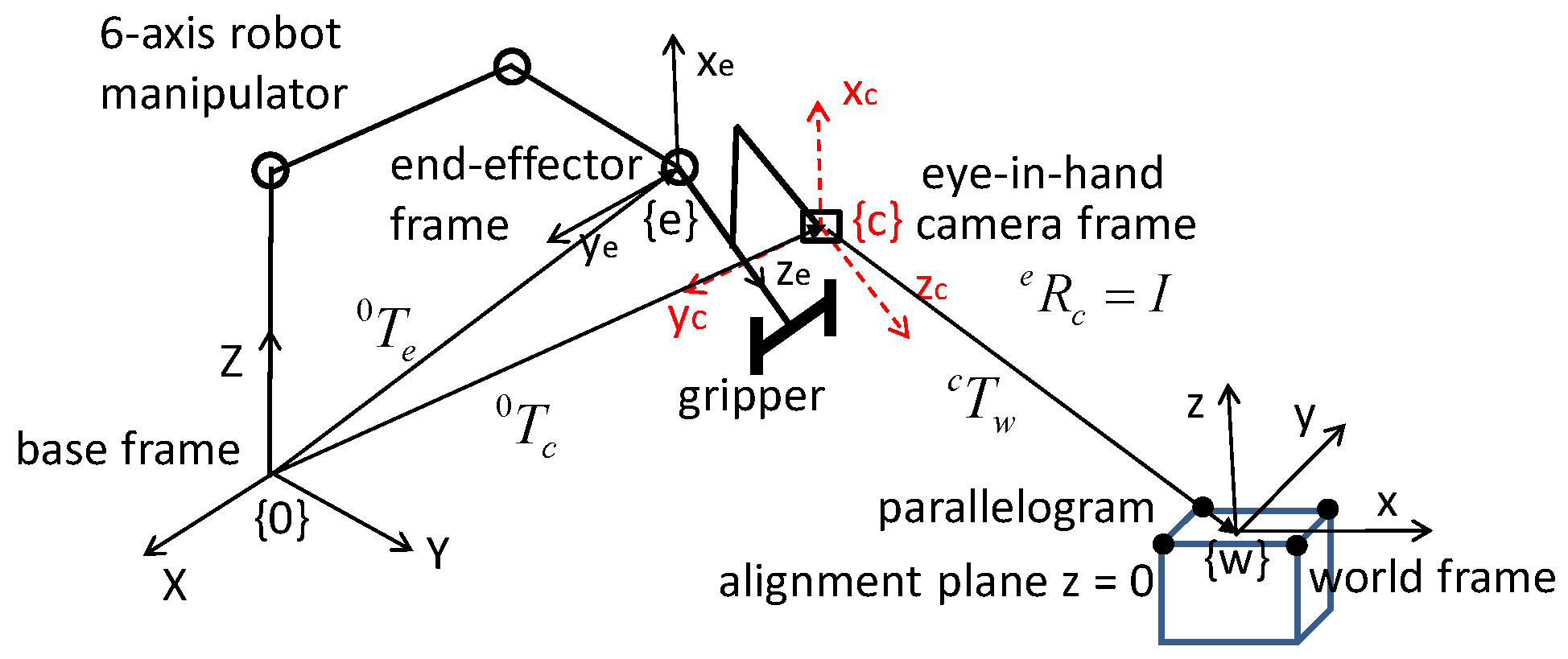
The coordinate frames of a 6-degrees of freedom (DOF) robot-gripper and single eye-in-camera system are defined as follows: the robot base coordinate frame {0}, end-effector coordinate frame {e}, eye-in-hand camera coordinate frame {c}, and world (or object/part) coordinate frame {w}. For simplicity, the eye-in-hand camera is installed so that the camera frame {c} and end-effector frame {e} are purely translational, and there is a rotational matrix ${}_{}{}^{e}R_c=I$.

Figure 1 shows coordinate systems of the robot-gripper-and-camera system. Position vectors $(X,Y,Z)$, $(x,y,z)$, $(x_c,y_c,z_c)$, and $(x_e,y_e,z_e)$ are the translation vector of a target position relative to the base frame {0}, world frame {w}, camera frame {c}, and end-effector frame {e}, respectively. Image point $(u,v)$ is a pixel coordinate in the image plane, such that the u-coordinate points to the $x_c$-axis and the v-coordinate points to the $y_c$-axis. Here, $R_x(\theta )$, $R_y(\theta )$, and $R_z(\theta )$ are defined as the basic rotational matrices of the rotational joints on the x-, y-, and z-axes.

The eye-in-hand camera 6-DOF pose estimation method is based on the camera pinhole model and the rigid transformation of a parallelogram in the world coordinate frame’s $z=0$ plane. The ideal pinhole camera model represents the relationship between the world space and the image space, while the relationship between the coordinate of the object point $(x,y,z)$ and the image point $(u,v)$ is given by

$$w\left[\begin{array}{c}u\\ v\\ 1\end{array}\right]=H\left[\begin{array}{c}x\\ y\\ 1\end{array}\right],$$

(1)

where the left-hand side ($w{[u,v,1]}^T$) is a homogeneous coordinate representation of the image space and H is a 3-by-3 homography matrix (or perspective projection matrix) up to a scale factor. A homograph is much easier to use for camera calibration with a flat world z = 0, than a general 3D case. A point (u,v) in the image corresponds to a certain point in the world.

The homography matrix H is a matrix multiplication of two 3-by-3 matrices:

$$H=AB,$$

(2)

where A is the camera intrinsic matrix, and B the extrinsic coordinate transformation B. The camera intrinsic matrix, $A=\left[\begin{array}{ccc}{k}_u& \gamma & u_0\\ 0& k_v& v_0\\ 0& 0& 1\end{array}\right]$, represents the relationship between the camera coordinate system and its image space. Parameters $k_u$ and $k_v$ are the effective focal length in pixels of the camera along the xc and yc directions, $\gamma$ is the camera skew factor, and $(u_0,v_0)$ is the coordinate of the principle point.

The extrinsic coordinate transformation matrix, $B=\left[\begin{array}{ccc}{r}_1& r_2& t\end{array}\right]$, represents the relationship between the camera coordinate system and the object coordinate system, the homogeneous matrix is ${}^{c}T_w=\left[\begin{array}{cc}R& t\\ 0^T& 1\end{array}\right]$, where $R=\left[\begin{array}{ccc}{r}_1& r_2& r_1\times r_2\end{array}\right]$, and the symbol $0^T$ stands for $[\begin{array}{ccc}0& 0& 0\end{array}]$. Here, it is assumed that the camera intrinsic matrix A is known in advance. There are several methods that can be applied to compute the camera intrinsic parameters, with Zhang’s plane target method [16] being a popular one.

Let ${\left[x_i,y_i,0\right]}^T$, $i=1,2,3,4$, be the alignment feature points in the world coordinate $z=0$ plane in the counter-clockwise direction, satisfying the parallelogram property, i.e., $x_1-x_2+x_3-x_4=0$ and $y_1-y_2+y_3-y_4=0$; and ${\left[u_i,v_i\right]}^T$, $i=1,2,3,4$, are the corresponding image points in the image plane. From the above four feature points ${\left[x_i,y_i,0\right]}^T$ and ${\left[u_i,v_i\right]}^T$, $i=1,2,3,4$, one can compute the parallelogram-to-quadrilateral projection homography H up to a scale factor. Moreover, if $u_1-u_2+u_3-u_4=0$ and $v_1-v_2+v_3-v_4=0$, then elements $H_{31}=H_{32}=0$, and H is a parallelogram-to-parallelogram affine transformation; otherwise, H is a perspective projection transformation. Affine transformation means the addition of translation to linear transformation. The properties of affine transformation include lines map to lines, parallel lines remain parallel, and parallelograms map to parallelograms. As a result, the object is lying in a plane parallel to the image plane. The alignment control can then be easily performed by translating in the x-y plane and rotating about the z-axis.

When the homography matrix H is an affine transformation, the absolute depth from camera to the object can be computed from

$$z_c=\frac{\sqrt{k_u{k}_v{S}_{xy}}}{\sqrt{S_{uv}}},$$

(3)

where $S_{xy}$ and $S_{uv}$ are the area of the parallelogram in the world space and in the image plane, respectively.

Once the projective matrix H has been computed, the extrinsic matrix B can be computed easily from

$$B=\left[\begin{array}{ccc}{r}_1& r_2& t\end{array}\right]=A^{-1}H.$$

(4)

The above matrix inverse approach does not enforce the orthonormality of the first two columns of the rotation matrix R, $R=\left[\begin{array}{ccc}{r}_1& r_2& r_1\times r_2\end{array}\right]$. One easy and approximate solution is to adjust them to orthonormality, by letting

$$\overline{B}=\left[\begin{array}{ccc}{\overline{r}}_1& {\overline{r}}_2& t\end{array}\right]=A^{-1}H,$$

(5)

and then setting

$$\begin{gathered} r_3=\frac{{\overline{r}}_1\times {\overline{r}}_2}{{\Vert {\overline{r}}_1\times {\overline{r}}_2\Vert }_2} \\ {r}_1=\frac{{\overline{r}}_2\times r_3}{{\Vert {\overline{r}}_2\times r_3\Vert }_2} \end{gathered}$$

and

$$r_2=r_3\times r_1$$

to satisfy $r_1^T{r}_2=0$ and $r_1^T{r}_1=r_2^T{r}_2=1$. Usage of the third orthogonal unit vector $r_3$ here is to guarantee that vectors $r_1$ and $r_2$ are orthogonal unit vectors. This simplified approach is easy to compute and acceptable, because we use the rotation matrix R merely as an estimate during the initially coarse vision alignment stage. The homogeneous matrix from the object coordinate system to the camera coordinate system is then

$${}^{c}T_w=\left[\begin{array}{cc}R& t\\ 0^T& 1\end{array}\right],\mathrm{and}R=\left[\begin{array}{ccc}{r}_1& r_2& r_1\times r_2\end{array}\right].$$

(6)

3. Positioning and Alignment Control in Pick-And-Place Tasks

As the camera is mounted on the robot end-flange, the relative position between the camera and the gripper is fixed. Moreover, the robot pose adjustment can be also regarded as an alignment of the camera pose with the part pose. The camera alignment control method is based on a coarse-to-fine strategy, in which position-based vision control is used in coarse alignment, followed by image-based fine alignment control.

3.1. Position-Based Coarse Vision Alignment

Let the part’s alignment pose respective to the camera frame be represented by ${}^{c}T_g=\left[\begin{array}{cc}{R}_g& t_g\\ 0^T& 1\end{array}\right]$, where $R_g=R_z({\theta }_g)$, and ${\theta }_g$ is the desired part orientation angle in the image plane, and $t_g$ is the desired part position relative to the camera frame. In a robot control system, the camera adjustment can be realized by a relative transformation matrix respective to the current camera frame {c}:

$${}^{c}T_c={}^{c}T_w{}^{c}T_g^{-1}.$$

(7)

The new camera pose is then changed according to

$${}^{0}T_c((k+1)T_s)={}^{0}T_c(k{T}_s){}^{c}T_c,$$

(8)

where $k{T}_s$ represents current time, and $(k+1)T_s$ represents the next pose updated time. Time $T_s$ is the robot’s point-to-point control play time, which was set in the range of 0.5~1.0 s in this study.

3.2. Image-Based Fine Alignment Control

As Equation (7) is based on the approximation condition, the above position-based alignment will not be precise to within a tolerable range for performing general robotic pick-and-place tasks, and further fine-alignment is required. Define $(u_g,v_g)=(u_0,v_0)$ as the desired target image position (center of the image plane), $h_g$ is the desired depth, and ${\theta }_g$ is the desired orientation angle in the image plane. Since the robot system has 6 degrees of freedom, one may define 6 control errors in the image space as follows:

$$\begin{gathered} e_1=\frac{u_1+u_2+u_3+u_4}{4}-u_0 \\ {e}_2=\frac{v_1+v_2+v_3+v_4}{4}-v_0 \\ {e}_3=u_1-u_2+u_3-u_4 \\ {e}_4=v_1-v_2+v_3-v_4 \\ {e}_5=\mathrm{atan}2(v_2-v_1,u_2-u_1)-{\theta }_g \end{gathered}$$

and

$$e_6=\frac{\sqrt{k_u{k}_v{S}_{xy}}}{\sqrt{S_{uv}}}-h_g.$$

Errors $(e_1,e_2)$ are used for compensating the parallelogram alignment positioning error, errors $(e_3,e_4)$ are used for compensating the parallelogram alignment orientation error, and the object depth and rotational errors $(e_5,e_6)$ are used mainly during the pick-and-place phase. The function of the control errors $(e_3,e_4)$ is to align with the object lying in a plane parallel to the image plane. Figure 2 shows the parallelogram alignment errors in the image space. A commonly adopted approach in visual servo control is the employment of simple proportional controllers.

To simplify the visual control design, the fine-alignment process is divided into two sub-systems. First, a proportional incremental control law,

$$\left[\begin{array}{c}\Delta x_c\\ \Delta y_c\end{array}\right]=\left[\begin{array}{c}{K}_1{e}_1\\ K_2{e}_2\end{array}\right],$$

(9)

is applied to align the center of the image parallelogram to the center position of the image plane, where $(\Delta x_c,\Delta y_c,0)$ is the incremental translation relative to the current camera coordinate frame. Second, a proportional incremental control law,

$$\left[\begin{array}{c}\Delta {\alpha }_c\\ \Delta {\beta }_c\end{array}\right]=\left[\begin{array}{c}{K}_3{e}_3\\ K_4{e}_4\end{array}\right],$$

(10)

is then applied to be used in camera fine-alignment control, where $(\Delta {\alpha }_c,\Delta {\beta }_c,0)$ are incremental rotation angles relative to the current camera coordinate frame. Proportional gains $K_1$ and $K_2$ are xy-plane translational error gains, and $K_3$ and $K_4$ are x-axis and y-axis rotational error gains during the fine-alignment control loop.

To select the proportional gains above, we need to look for the image Jacobian and examine system stability. Let $\nu ={[v_x,v_y,v_z]}^T$ and $\omega ={[{\omega }_x,{\omega }_y,{\omega }_z]}^T$ be the translation linear speed and rotation angular speed of the eye-in-hand camera with respect to camera frame. The image Jacobian of a point object P at camera coordinate $(x_c,y_c,z_c)$ and image coordinate $(u,v)$ can be represented by

$$\left[\begin{array}{c}\dot{\overline{u}}\\ \dot{\overline{v}}\end{array}\right]=\left[\begin{array}{cccccc}-\frac{k_u}{z_c}& 0& \frac{\overline{u}}{z_c}& \frac{\overline{u}\overline{v}}{k_v}& -k_u-\frac{{\overline{u}}^2}{k_u}& \frac{k_u}{k_v}\overline{v}\\ 0& -\frac{k_v}{z_c}& \frac{\overline{v}}{z_c}& k_v+\frac{{\overline{v}}^2}{k_v}& -\frac{\overline{v}\overline{u}}{k_u}& -\frac{k_v}{k_u}\overline{u}\end{array}\right]\left[\begin{array}{c}\nu \\ \omega \end{array}\right],$$

(11)

where $\overline{u}=u-u_0$ and $\overline{v}=v-v_0$.

The parallelogram position alignment error can be rewritten as

$$\left[\begin{array}{c}{e}_1\\ e_2\end{array}\right]=\left[\begin{array}{c}(u_1+u_2+u_3+u_4)/4-u_0\\ (v_1+v_2+v_3+v_4)/4-v_0\end{array}\right]=\left[\begin{array}{c}({\overline{u}}_1+{\overline{u}}_2+{\overline{u}}_3+{\overline{u}}_4)/4\\ ({\overline{v}}_1+{\overline{v}}_2+{\overline{v}}_3+{\overline{v}}_4)/4\end{array}\right],$$

(12)

and from the image Jacobian matrix in Equation (11), one can obtain

$$\left[\begin{array}{c}{\dot{e}}_1\\ {\dot{e}}_2\end{array}\right]=\left[\begin{array}{cc}-k_u{z}_c^{-1}& 0\\ 0& -k_v{z}_c^{-1}\end{array}\right]\left[\begin{array}{c}{v}_x\\ v_y\end{array}\right].$$

(13)

It is clear that the proportional control law in Equation (9), $\left[\begin{array}{c}{v}_x\\ v_y\end{array}\right]=\left[\begin{array}{c}{K}_1{e}_1\\ K_2{e}_2\end{array}\right]$, $K_1,K_2>0$, derives the steady-state error $(e_1,e_2)$ to zero for static objects.

The parallelogram orientation alignment error can also be rewritten as

$$\left[\begin{array}{c}{e}_3\\ e_4\end{array}\right]=\left[\begin{array}{c}{u}_1-u_2+u_3-u_4\\ v_1-v_2+v_3-v_4\end{array}\right]=\left[\begin{array}{c}{\overline{u}}_1-{\overline{u}}_2+{\overline{u}}_3-{\overline{u}}_4\\ {\overline{v}}_1-{\overline{v}}_2+{\overline{v}}_3-{\overline{v}}_4\end{array}\right],$$

(14)

and

$$\left[\begin{array}{c}{\dot{e}}_3\\ {\dot{e}}_4\end{array}\right]=\left[\begin{array}{cc}\frac{{\overline{u}}_1{\overline{v}}_1-{\overline{u}}_2{\overline{v}}_2+{\overline{u}}_3{\overline{v}}_3-{\overline{u}}_4{\overline{v}}_4}{k_v}& -\frac{{\overline{u}}_1^2-{\overline{u}}_2^2+{\overline{u}}_3^2-{\overline{u}}_4^2}{k_u}\\ \frac{{\overline{v}}_1^2-{\overline{v}}_2^2+{\overline{v}}_3^2-{\overline{v}}_4^2}{k_v}& -\frac{{\overline{u}}_1{\overline{v}}_1-{\overline{u}}_2{\overline{v}}_2+{\overline{u}}_3{\overline{v}}_3-{\overline{u}}_4{\overline{v}}_4}{k_u}\end{array}\right]\left[\begin{array}{c}{\omega }_x\\ {\omega }_y\end{array}\right].$$

(15)

The proportional control law in Equation (10), $\left[\begin{array}{c}{\omega }_x\\ {\omega }_y\end{array}\right]=\left[\begin{array}{c}{K}_3{e}_3\\ K_4{e}_4\end{array}\right]$ is used only when $e_1=e_2=0$, and we have

$$\left[\begin{array}{c}{\dot{e}}_3\\ {\dot{e}}_4\end{array}\right]=\left[\begin{array}{cc}{K}_3\frac{{\overline{u}}_1{\overline{v}}_1-{\overline{u}}_2{\overline{v}}_2+{\overline{u}}_3{\overline{v}}_3-{\overline{u}}_4{\overline{v}}_4}{k_v}& -K_3\frac{{\overline{u}}_1^2-{\overline{u}}_2^2+{\overline{u}}_3^2-{\overline{u}}_4^2}{k_u}\\ K_4\frac{{\overline{v}}_1^2-{\overline{v}}_2^2+{\overline{v}}_3^2-{\overline{v}}_4^2}{k_v}& -K_4\frac{{\overline{u}}_1{\overline{v}}_1-{\overline{u}}_2{\overline{v}}_2+{\overline{u}}_3{\overline{v}}_3-{\overline{u}}_4{\overline{v}}_4}{k_u}\end{array}\right]\left[\begin{array}{c}{e}_3\\ e_4\end{array}\right].$$

(16)

To examine stability, let $V=\frac{1}{2}{e}_3^2+\frac{1}{2}{e}_4^2$, be a candidate of the Lyapunov function and thus when positive definite conditions

$$\begin{gathered} -K_3\frac{{\overline{u}}_1{\overline{v}}_1-{\overline{u}}_2{\overline{v}}_2+{\overline{u}}_3{\overline{v}}_3-{\overline{u}}_4{\overline{v}}_4}{k_v}\ge 0,\mathrm{and} \\ -K_3{K}_4\frac{{({\overline{u}}_1{\overline{v}}_1-{\overline{u}}_2{\overline{v}}_2+{\overline{u}}_3{\overline{v}}_3-{\overline{u}}_4{\overline{v}}_4)}^2-({\overline{u}}_1^2-{\overline{u}}_2^2+{\overline{u}}_3^2-{\overline{u}}_4^2)({\overline{v}}_1^2-{\overline{v}}_2^2+{\overline{v}}_3^2-{\overline{v}}_4^2)}{k_v{k}_u}>0 \end{gathered}$$

are satisfied, we have asymptotic stability. Recalling that ${\overline{u}}_1+{\overline{u}}_3+{\overline{u}}_2+{\overline{u}}_4=0$ and ${\overline{v}}_1+{\overline{v}}_3+{\overline{v}}_2+{\overline{v}}_4=0$, it can be shown that

$$\begin{gathered} {({\overline{u}}_1{\overline{v}}_1-{\overline{u}}_2{\overline{v}}_2+{\overline{u}}_3{\overline{v}}_3-{\overline{u}}_4{\overline{v}}_4)}^2-({\overline{u}}_1^2-{\overline{u}}_2^2+{\overline{u}}_3^2-{\overline{u}}_4^2)({\overline{v}}_1^2-{\overline{v}}_2^2+{\overline{v}}_3^2-{\overline{v}}_4^2) \\ ={({\overline{u}}_1{\overline{v}}_2-{\overline{v}}_1{\overline{u}}_2+{\overline{u}}_2{\overline{v}}_3-{\overline{v}}_2{\overline{u}}_3+{\overline{u}}_3{\overline{v}}_1-{\overline{u}}_1{\overline{v}}_3)}^2>0. \end{gathered}$$

Thus, to derive the steady-state error $(e_3,e_4)$ to zero, it is required that: $K_3=-\mathrm{sgn}({\overline{u}}_1{\overline{v}}_1-{\overline{u}}_2{\overline{v}}_2+{\overline{u}}_3{\overline{v}}_3-{\overline{u}}_4{\overline{v}}_4)K$, $K>0$, and $K_4=-K_3$.

When $e_1=e_2=0$ and $e_3=e_4=0$, the camera is moved to the upright position of the target plane $z=0$; after this, the absolute depth from camera to the object, $z_c$, can be computed precisely from Equation (3). The proportional control law,

$$\left[\begin{array}{c}\Delta {\theta }_c\\ \Delta z_c\end{array}\right]=\left[\begin{array}{c}{K}_5{e}_5\\ K_6{e}_6\end{array}\right],$$

(17)

is then applied to perform the pick-and-place tasks.

3.3. Camera Pose Alignment and Robot Pick-And-Place Sequential Control

The eye-in-hand camera alignment control and robot pick-and-place task are executed by simple sequential control. Coarse camera alignment is carried out and followed immediately by fine camera alignments, finishing up with a pick-and-place of the part by the gripper. The detailed alignment and pick-and-place procedure are listed and explained below.

Step 1:

Position-based camera coarse-alignment as stated in Section 3.1.

Step 2:

Image-based camera fine-alignments (refer to Section 3.2).

Step 2.1:

Compensation of position error by moving the camera pose relative to the current camera frame, ${}^{c}T_c=\left[\begin{array}{cc}I& \Delta p_c\\ 0^T& 1\end{array}\right]$, where $\Delta p_c={\left[\Delta x_c,\Delta y_c,0\right]}^T$. The new camera pose is then changed according to ${}^{0}T_c((k+1)T_s)={}_{0}T{}_c(k{T}_s){}_{c}T{}_c$.

If $\max \{\left|e_1\right|,\left|e_2\right|\}>\epsilon$, then repeat Step 2.1; else if $\max \{\left|e_3\right|,\left|e_4\right|\}>\delta$, then go to Step 3; else go to Step 2.2.

Step 2.2:

Compensate orientation error by rotating the camera pose with respect to the current camera frame x- and y-axes, ${}^{c}T_c=\left[\begin{array}{cc}{}^{c}R_c& 0\\ 0^T& 1\end{array}\right]$, where ${}^{c}R_c=R_x(\Delta {\alpha }_c)R_y(\Delta {\beta }_c)$. The new camera pose is then changed according to ${}^{0}T_c((k+1)T_s)={}^{0}T_c(k{T}_s){}^{c}T_c$.

If $\max \{\left|e_3\right|,\left|e_4\right|\}>\delta$, then repeat Step 2.2; else go to Step 2.1.

Step 3:

Execute robot gripper pick-and-place motion relative to current end-effector frame, ${}^{e}T_e=\left[\begin{array}{cc}{}^{e}R_e& \Delta p_e\\ 0^T& 1\end{array}\right]$, where ${}^{e}R_e=R_z(\Delta {\theta }_c)$ and $\Delta p_e={\left[\Delta x_e,\Delta y_e,\Delta z_e\right]}^T$. The gripper pose is then changed according to ${}^{0}T_e((k+1)T_s)={}^{0}T_e(k{T}_s){}^{e}T_e$.

4. Experimental Results and Discussions

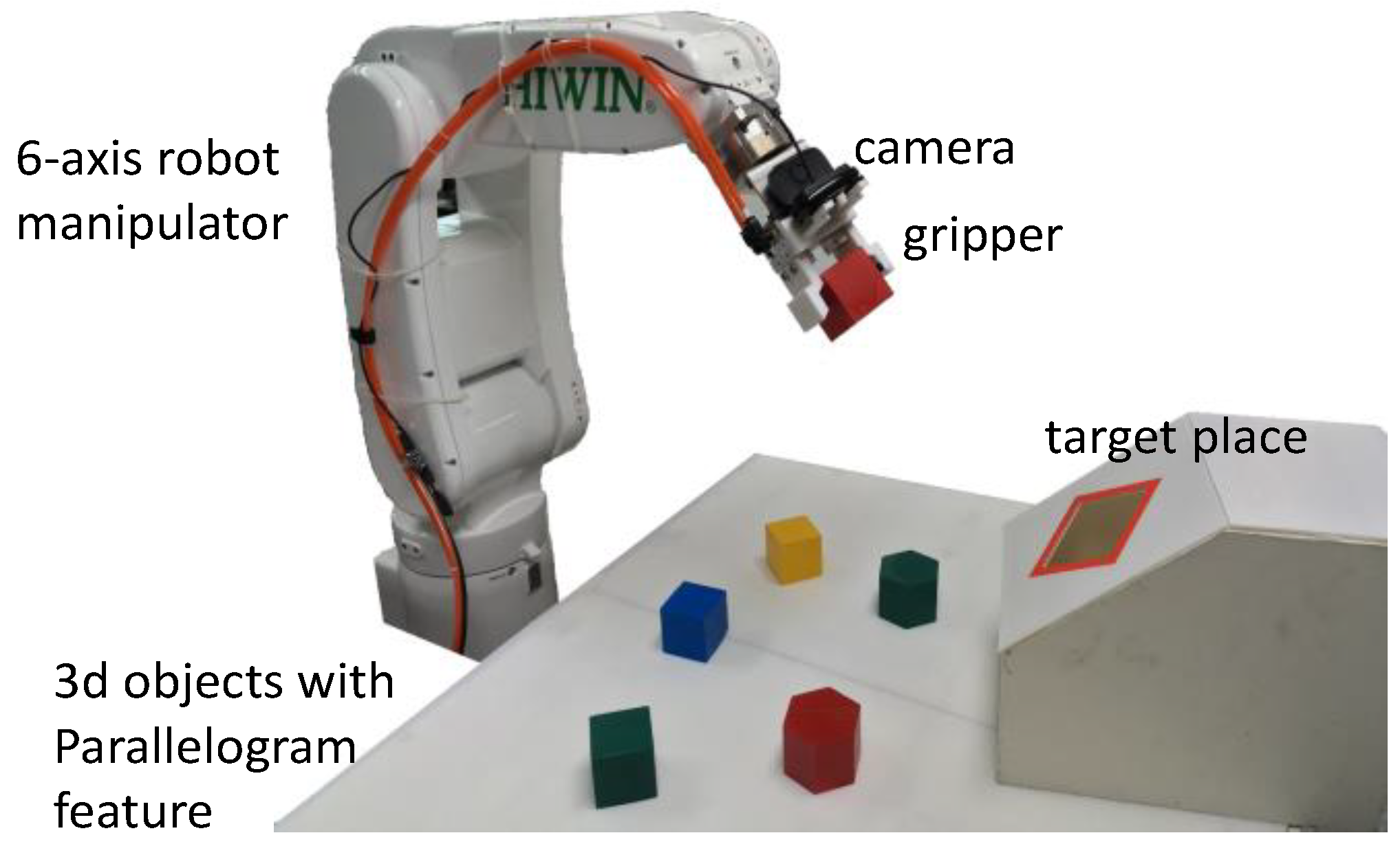
The experimental robot used in this study was a Hiwin R605 6-axis industrial manipulator, which had an on–off gripper attached to its end-effector. A camera was installed on a fixed end-flange in front of and above the gripper. The eye-in-hand camera used was a low-cost Web color camera with a resolution of 720 × 1280 at 30 fps. The overall robot control system was based on a commercially provided robot controller running under a continuous look-and-move control strategy. The robot controller had built-in set-point control and point-to-point motion control utilities in both joint-space and Cartesian-space. We implement the robot vision and control software on a PC with Microsoft Visual C++ programming language and use OpenCV library functions, such as cvtColor, findContours, and approxPolyDP, for color segmentation and to search for an object’s vertices.

Figure 3 shows the experimental robot control system set-up, in which the geometric data of the 3D objects are known. Each packing part or target placing location is featured by a parallelogram.

Table 1. Intrinsic camera parameters.

Parameter	${\mathit{k}}_{\mathit{u}}$	${\mathit{k}}_{\mathit{v}}$	$\mathit{\gamma }$	${\mathit{u}}_0$	${\mathit{v}}_0$
Value	985.03	984.62	0.0	378.33	619.76

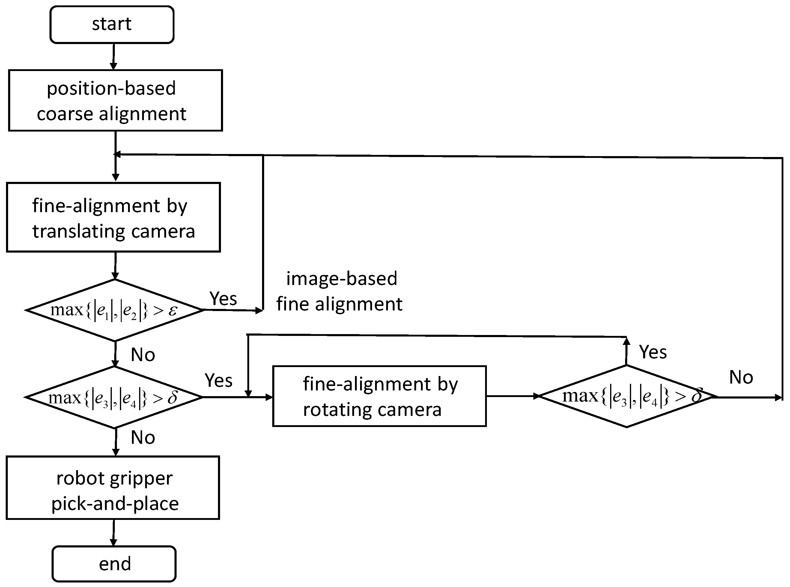
shows the camera’s intrinsic parameters. As the eye-in-hand camera is moving and close to the estimated object, the camera skew factor $\gamma =0$. Figure 4 is a schematic of the control flow of the eye-in-hand camera alignment control and gripper pick-and-place control.

Table 2. Proportional control gains.

Gain	${\mathit{K}}_1$	${\mathit{K}}_2$	${\mathit{K}}_3$	${\mathit{K}}_4$	${\mathit{K}}_5$	${\mathit{K}}_6$
Value	0.2463	0.2463	$-$0.3175	0.3175	1	1

shows the proportional incremental control gains in image-based fine-alignment control. Since the unit of $e_5$ is angle error (in degrees) and that of $e_6$ is depth error (in mm), $K_5=1$ and $K_6=1$ are used.

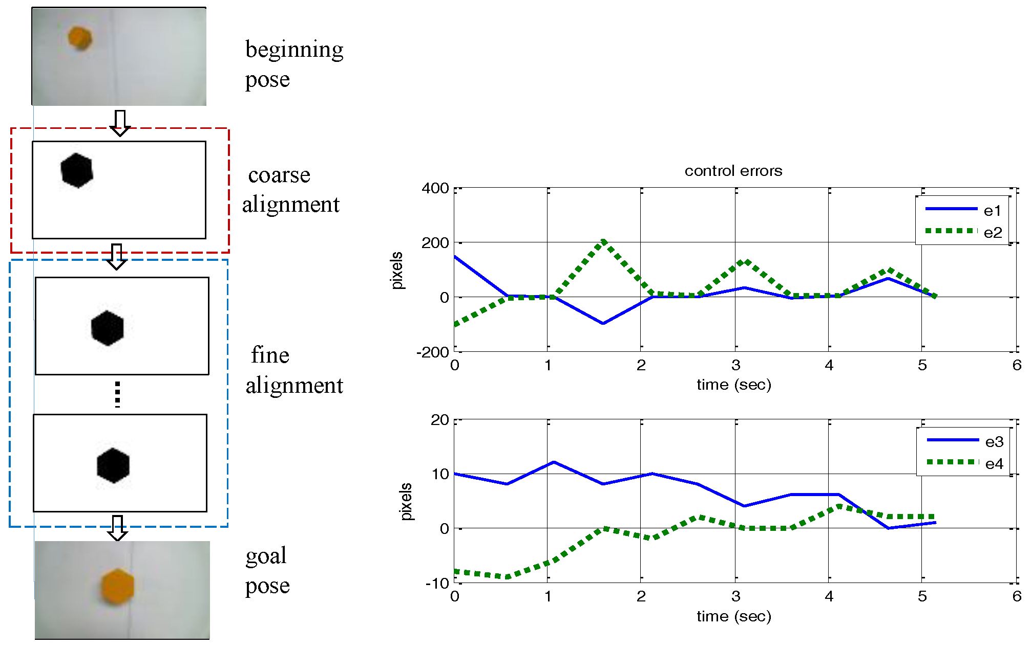
In the first alignment control experiment, the goal was to align the camera with a hexahedron part at the center and upright position in the image plane and then to cause the robot to pick up the part. Figure 5 shows the camera alignment control result for picking up the part. The alignment goal pose is set to:

$${}^{c}T_g=\left[\begin{array}{cccc}1& 0& 0& 0\\ 0& 1& 0& 0\\ 0& 0& 1& 200\\ 0& 0& 0& 0\end{array}\right],$$

and the external parameters matrix at the beginning pose was computed as

$${}^{c}T_w=\left[\begin{array}{cccc}0.926577& 0.327094& -0.185648& 61.5127\\ -0.209547& 0.858864& 0.467378& -121.6251\\ 0.312323& -0.394159& 0.864346& 474.4364\\ 0& 0& 0& 1\end{array}\right].$$

The coarse alignment control motion was then set as ${}^{c}T_c={}^{c}T_w{}^{c}T_g^{-1}$.

The error bounds were then set to $\epsilon =4$ pixels and $\delta =2$ pixels for the following fine-alignment stage. After eight fine-alignment movements, the camera moved to the upright center position of the hexahedron at a depth of 200 mm. The positioning accuracy was within 1.0 mm and the orientation angle accuracy was within 1.0 degree. The robot vision control system follows a continuous look-and-move control scheme. The processing time of the object feature vision feedback is less than one second. In each vision control iteration, the robot’s movement follows a joint space point-to-point motion with set-points obtained from the vision control law and the robot’s inverse kinematics. Usually, a joint space point-to-point motion takes 0.5 to 1.0 s. The alignment control finishes within three iterations on average, and thus the vision-based alignment control task takes just a few seconds.

In the second alignment control experiment, the goal was to first align the camera with a square shape at the center and upright position in the image plane and then to cause the robot to place the object. Figure 6 shows the camera alignment control result before placing the object. The goal alignment pose was set to

$${}^{c}T_g=\left[\begin{array}{cccc}1& 0& 0& 0\\ 0& 1& 0& 0\\ 0& 0& 1& 300\\ 0& 0& 0& 0\end{array}\right],$$

and the external parameters matrix at the beginning pose was computed as

$${}^{c}T_w=\left[\begin{array}{cccc}0.987708& -0.001122& -0.156303& 122.4860\\ -0.108232& 0.716561& -0.689076& -153.3283\\ 0.112774& 0.697523& 0.707632& 564.0036\\ 0& 0& 0& 1\end{array}\right].$$

The coarse alignment control motion was then set as ${}^{c}T_c={}^{c}T_w{}^{c}T_g^{-1}$.

In the fine-alignment stage, the error bounds were also set to $\epsilon =4$ pixels and $\delta =2$ pixels. After 7 fine-alignment movements, the camera is moved to the upright center position of the square shape at a depth of 300 mm. The positioning accuracy was within 1.0 mm and orientation angle accuracy was within 1.0 degree.

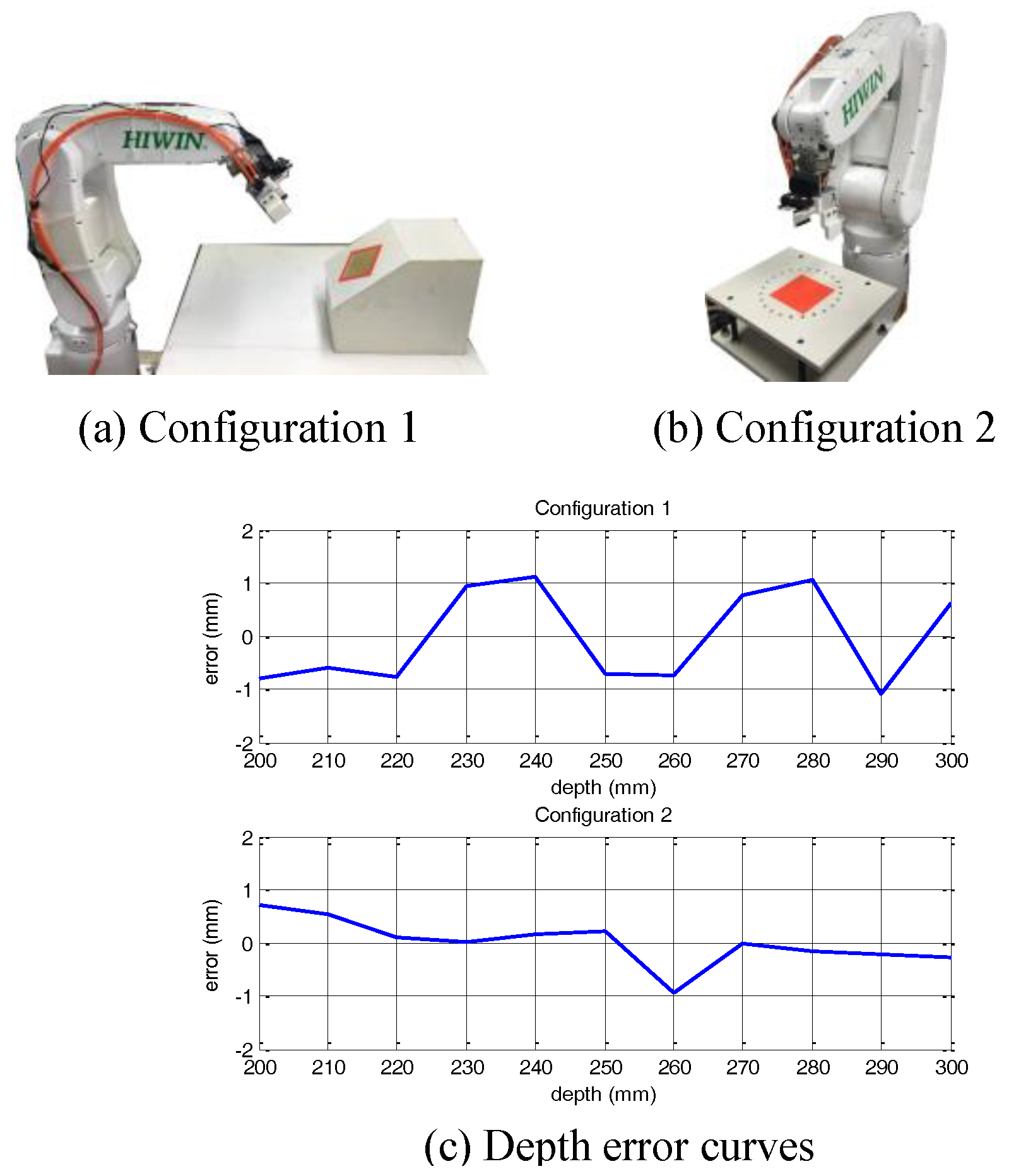
In the following depth error experiment, the approximate distance from the camera location to the object was between 200 mm and 300 mm during pose estimation. Figure 7 shows the computed depth error, using Equation (3), for two different object poses after fine-alignment was done. The actual depth error was about 1.2 mm.

We next discuss the main advantages and disadvantages of similar eye-in-hand visual servo control systems, in which the target object is composed of four non-coplanar points, and perform experimental tests on a 6-DOF robot [6,17,18]. We base the use of four characteristic points in total for six DOFs on a commonly used strategy. From the projection of these four points in the image frame, a set of six features can control all six DOFs of the robot manipulator: three for positioning control and three for orientation control.

The work by Hager uses projective geometry and projective invariance in robotic hand-eye coordination [6]. This approach separates hand-eye coordination into application-independent hand-eye utilities and application-dependent geometric operations. The three basic position/alignment skills are planar positioning, parallel alignment, and positioning in the object coordinate. The experiments are based on tracking corners formed by the intersections of line segments. The accuracy of the placement is typically within 2.0 mm. Because all of the proposed control algorithm are nonlinear, this approach sometimes exhibits singularities within a viewable workspace.

Kosmopoulos experimented with a 6-DOF sunroof placement robot by monitoring four corners of a sunroof opening [17]. That research identified the corners as the interaction points of the two line edges. The sunroof placement installation operation is thus done under a small workspace volume. The visual control system does not need to estimate the depth and there is no need for camera calibration. The control method is based on a local calculation of the image Jacobian matrix through training and is only suitable for relatively small deviations (10.0 mm and 1.0 degrees) from the end-effector nominal pose.

Recent work by Keshmiri and Xie combines optimized trajectory planning with an augmented image-based servo control [18], using six visual features to facilitate the optimization procedure and depth-estimation. These features are the center of four feature points, the perimeter of the lines connecting each consecutive feature point, and three rotational angles from the deformation in the features by rotating the camera about its x-axis, y-axis and z-axis. The planning procedure consists of three stages: moving the camera to estimate the depth of features, planning the best camera velocity to remove orientation errors, and planning the best camera velocity to remove position errors. A calibration error could deviate the robot from its ideal path, and the local minima problem may arise. Because this is global offline trajectory planning, it is therefore unable to work in a dynamically changing environment.

The main advantage of the proposed methodology is the simplicity of implementing the visual servo control without using the interaction matrix as a traditional method. Our method is based on the point error and area error of four feature points. We choose the parallelogram model so as to capture any interesting features for use in the 6-DOF imaged-based visual servo control. The positioning and alignment task employs only simple parallelism invariance and decoupled proportional control laws to position and align the camera with a target object. An accurate absolute depth, from the camera to the object, can be obtained from its area in the image space. Experimental results show excellent applicability of the proposed approach for pick-and-place tasks, and the overall errors are 1.2 mm for positioning and 1.0° for orientation angle.

5. Conclusions

This paper describes a simple and efficient method for camera positioning and alignment control using a single eye-in-hand camera. The proposed technique uses simple parallelism invariance to align the eye-in-hand camera with a part based on a coarse and fine alignment strategy. Accurate absolute depth from camera to the part can be obtained from its area in the image space. The overall positioning accuracy is within 1.2 mm and orientation angle accuracy is within 1.0 degree. The main advantages of the proposed visual servoing are as follows: (1) easy implementation and less calibration; (2) a planar image feature based on parallelism without the need to compute the image Jacobian matrix; and (3) the ability to measure precise absolute depth information by a single eye-in-hand camera. As the proposed approach is based on a parallelogram feature, it does not work with arbitrary-shaped objects. However, the proposed method can be applicable to an object that is adhered to a parallelogram marker or an object’s interior that has the four vertices of a parallelogram (such as a hexagon and octagon). We only use a parallelogram in a planar plane as the key image feature herein.

In a future work, we will employ the invariant cross-ratio to invariantly position a point with respect to a projective basis on a line—for instance, generating points on a 3D line using measured image cross-ratios. Furthermore, a quadrilateral in an image form four-point basis can be used directly for the generation of coplanar 3D points. In this work the pick-and-place task is constrained to 2-1/2D objects, and object geometric data are known in advance. Due to the image processing techniques used and the limited usage of a commercial robot controller in linear motion, the speed of pick-and-place tasks in our experiment was quite slow. Further work can include estimation of the pose of general 3D objects without knowing their geometric data, and conducting faster pick-and-place tasks.