On a Two-DoF Parallel and Orthogonal Variable-Stiffness Actuator: An Innovative Kinematic Architecture

Abstract

Variable-Stiffness Actuators are continuously increasing in importance due to their characteristics that can be beneficial in various applications. It is undisputed that several one-degree-of-freedom (DoF) solutions have been developed thus far. The aim of this work is to introduce an original two-DoF planar variable-stiffness mechanism, characterized by an orthogonal arrangement of the actuation units to favor the isotropy. This device combines the concepts forming the basis of a one-DoF agonist-antagonist variable-stiffness mechanism and the rigid planar parallel and orthogonal kinematic one. In this paper, the kinematics and the operation principles are set out in detail, together with the analysis of the mechanism stiffness.

1. Introduction

A Variable-Stiffness Actuator (VSA) permits the adjustment of both the position and stiffness of the load [1]. The fundamental aspects of a VSA are: (i) real-time adjustable stiffness requiring neither force sensors nor transmission backdrivability; (ii) robustness to external perturbations and unpredictable model errors; (iii) adaptability and force accuracy in the interaction with the operator; (iv) suitable for direct interaction with humans in the presence of safety requirements, limiting the force of collisions in the event of a malfunction or unexpected movements.

The above aspects, as well as the onset of new field of applications, are making them increasingly viable solutions. In fact, a first attempt to organize the numerous available technologies and solutions presented in the scientific literature was considered necessary and fundamental to establish a common language for designers and potential users [2]. Different types of VSA actuation schemes have been developed thus far [1,3]. In particular, it is worth mentioning, the so-called principle of operation of the agonist-antagonist [4], commonly used in such devices and adapted to the kinematic architecture set out in the present work.

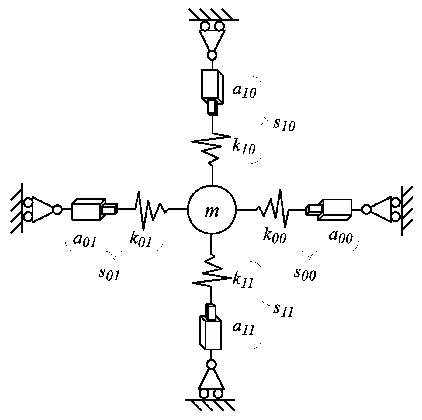
Usually these are made up of two Series Elastic Actuators (SEA) arranged in parallel to a mobile mass as shown in Figure 1. SEAs are constituted by a rigid actuator and a non-linear spring assembled serially [5]. The nonlinearity of the elastic element is necessary to allow the adjustment of the VSA stiffness [6]. Non-linear springs can be realized in different ways. An example of these, are non-homogeneous coil springs, obtained by varying the pitch or the diameter along the axis. With the same objective an alternative solution would be to employ cams with variable-radius, e.g., [7,8]. In fact, the vast majority of the VSAs developed thus far are characterized by a one-DoF actuation scheme. To the authors’ knowledge only one two-DoF mechanism enabling planar movements has been developed up to now [9]. This is a cable-driven device arranged on a triangular framework, with three non-linear SEAs. Due to the presence of three tendons, the possibility to adjust the stiffness of the load along different directions is limited. Moreover, each tendon is controlled independently by two actuators, thus requiring six of these.

To take the existing architecture one step further and enhance the isotropy in terms of stiffness and decoupling of degrees of freedom, an original kinematics two-DoF planar solution based on two orthogonal tendon-driven VSA actuation schemes was developed and is presented in this work. Its original kinematics allows one to tune, at the same time, both the equilibrium position and the stiffness of a mobile platform along two orthogonal directions. The orthogonal configuration is an arrangement that helps to reach an isotropic behavior in the entire workspace [10,11,12].

Moreover, the architecture has been conceived with the aim of minimizing the number of actuators required. In fact, the architecture presented within this work uses only four actuators, being the minimum number required to control both the equilibrium position and the mechanical stiffness of a mobile mass along two orthogonal directions. Combining the typical modularity of VSA antagonist actuators, the architecture presented herein is essentially made up of two orthogonal VSAs, as shown in the scheme set out in Figure 2, within which each one of these are characterized by two antagonist identical submodules.

The paper is organized as follows: the nomenclature is listed in

Table 1. Table of symbols.

Symbol	Description
$P_{\cdots }$	Geometric point
$\left\{f\right\}$	Reference frame. $\left\{w\right\}$ denotes the global reference frame.
${\mathbf{P}}_{\cdots \left(f\right)}=$, ${[P_{\cdots ,x\left(f\right)},P_{\cdots ,y\left(f\right)}]}^T$	Coordinates x and y of point $P_{\cdots }$ WRT $\left\{f\right\}$. If no $\left\{f\right\}$ is indicated, $\left\{w\right\}$ is understood.
$\dot{\mathbf{P}}$	First time derivative of P
${\mathbf{O}}_f$	Origin of $\left\{f\right\}$
$\{{\mathbf{e}}_{f,x},{\mathbf{e}}_{f,y}\}$	Axes of $\left\{f\right\}$
$d(P,Q)$	Distance between point P and Q
$\mathbf{v}={[v_{x\left(f\right)},v_{y\left(f\right)}]}^T$, $\mathbf{v}=v{\mathbf{u}}_v$	Vector v, with components $v_{x\left(f\right)}$ and $v_{y\left(f\right)}$ WRT $\left\{f\right\}$, of magnitude v and direction ${\mathbf{u}}_v$
$\mathbf{v}(Q,P)=\mathbf{Q}-\mathbf{P}$	Vector from P to Q applied in P.
$\mathbf{U}(Q,P)=\frac{\mathbf{v}(Q,P)}{\left|\mathbf{v}\right(Q,P\left)\right|}$	Unit vector from P toward Q.
$\mathbf{u}\left(\mathbf{v}\right)=\frac{\mathbf{v}}{\left|\mathbf{v}\right|}$	Unit vector of v.

; the kinematic architecture is presented in Section 2; the force and stiffness analysis is described in Section 3; conclusions are drawn in Section 4.

2. Kinematics

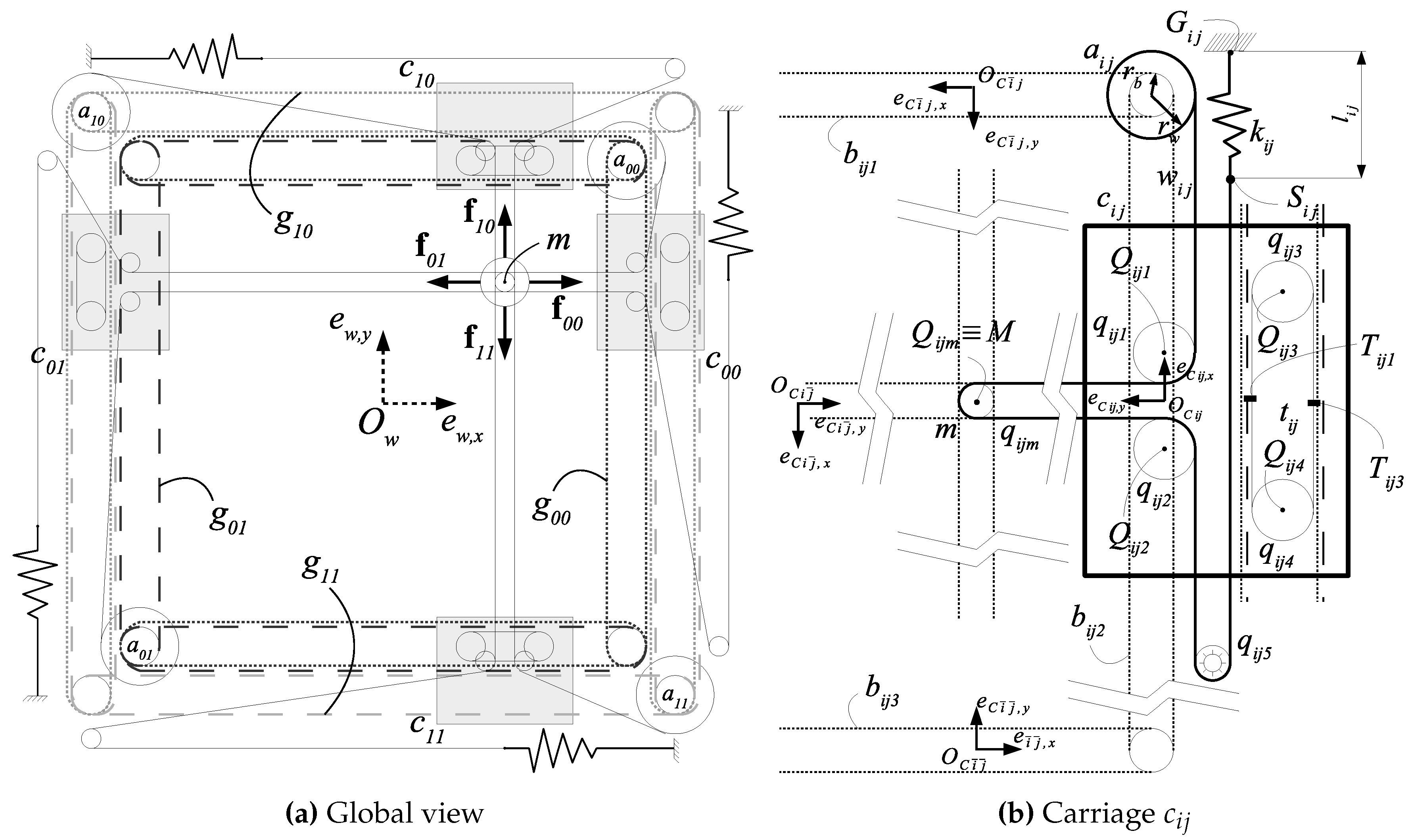
Let us refer to Figure 3 and to Figure 4 for a graphical representation of the kinematic architecture under consideration. The former is a simplified scheme of two main embedded submodules. The latter is a completed scheme of all the main components and sets out all the required symbols for a complete geometrical and analytic description.

The two-DoF planar VSA presented in this work is made up of four almost identical actuation modules, orthogonal and antagonistic in pairs, identified by $g_{ij}$, where $i\in \{0,1\}$ and $j\in \{0,1\}$. The subscripts $\left(ij\right)$ indicate hereafter both the direction and the orientation with respect to $\left\{w\right\}$, being the global planar reference frame. This notation has been chosen for the sake of generality. Nevertheless, referring to Figure 4, the subscript i is the actuation direction and, specifically, $i=0$ and $i=1$ correspond to $i={\mathbf{e}}_{w,x}$ and $i={\mathbf{e}}_{w,y}$, respectively, whereas, the subscript j refers to its orientation and, specifically, $j=0$ and $j=1$ correspond to the same or the opposite orientation of the specified i unit vector, respectively. Moreover, let us define $\overline{i}$ and $\overline{j}$ the complement to 1 of i and j, respectively. Accordingly, given that $g_{ij}$ refers to, generically, one of the four actuation modules, $g_{\overline{i}j}$ and $g_{\overline{i}\overline{j}}$ refer to the two actuation modules perpendicular to $g_{ij}$ and antagonists between them.

A mobile body m is connected to the ground by means of four wires $w_{ij}$ tensioned by non-linear springs $k_{ij}$, each of these belonging to $g_{ij}$. Wires $w_{ij}$ are wrapped around four pulleys concentric to the center of m, indicated by M.

By hypothesizing that the inertial and external forces acting on m are disregarded, this system configuration shows the characteristic of applying to m a set of forces ${\mathbf{f}}_{ij}$, parallel to i with orientation j, antagonist and orthogonal in pairs.

The generic module $g_{ij}$ is made up of:

• a rotational actuator $a_{ij}$ characterized by the rotational coordinate ${\theta }_{ij}$ and the torque ${\tau }_{ij}$;
• a non-linear spring $k_{ij}$, assumed to be identical $\forall i,j$, with length $l_{ij}=d(S_{ij},G_{ij})=\Delta l_{ij}+l_{ij,eq}$, indicating $G_{ij}$ as ground point, $S_{ij}$ the free endpoint of $w_{ij}$, $l_{ij,eq}$ the preload length of the spring, and $\Delta l_{ij}$ the length variation from the preload length;
• a wire $w_{ij}$ actuated by $a_{ij}$ at one of its endpoints, exerting on M the pulling force ${\mathbf{f}}_{ij}$ due to the elongation of $k_{ij}$;
• a carriage $c_{ij}$, ensuring the correct direction of ${\mathbf{f}}_{ij}$;
• a set of synchronous belts $b_{ijl}$, with $l\in \{1,2,3\}$, with the task of synchronizing the motion of the carriages $c_{\overline{i}j}$ and $c_{\overline{i}\overline{j}}$ with respect to M thus assuring the orthogonality of the antagonist force pairs (${\mathbf{f}}_{\overline{i}j}$ and ${\mathbf{f}}_{\overline{i}\overline{j}}$) acting on the end effector.

As can be seen from Figure 4a, the only difference between $g_{0j}$ and $g_{1j}$ (for each j) is the length of belts $b_{ijl}$ for assembly purposes. We can moreover denote:

• ${\mathbf{f}}_m$ the external force applied to m;
• $v_i$ each couple $(g_{i0},g_{i1})$ constituting an antagonistic VSA.

Referring to Figure 5 and ignoring inertial effects, the position of m (i.e., M) can be obtained by solving the equilibrium equation:

$$\sum _{i=1}^2\sum _{j=1}^2{\mathbf{f}}_{ij}+{\mathbf{f}}_m={\mathbf{f}}_s+{\mathbf{f}}_m=0.$$

(1)

where ${\mathbf{f}}_s$ denotes the total force exerted by the springs on m.

The mechanical transmission of this architecture, constituted by $c_{ij}$, $w_{ij}$ and $b_{ijl}$, ensures that the forces applied to m are orthogonal and antagonistic in pairs, as set out below (Figure 4):

$${\mathbf{f}}_{01}=-{\mathbf{f}}_{00},{\mathbf{f}}_{11}=-{\mathbf{f}}_{10},{\mathbf{f}}_{00}\perp {\mathbf{f}}_{10},$$

(2)

and assuming that all $k_{ij}$ are identical and no external forces are applied, i.e., ${\mathbf{f}}_m=\mathbf{0}$. This is an aspect which can be anticipated to control both the equilibrium position and the stiffness of m along two orthogonal directions in performing planar movements.

We will now focus on the generic carriage $c_{ij}$ to illustrate the transmission mechanism represented in Figure 4b where $\left\{c_{ij}\right\}$ denotes its local reference frame. Each $c_{ij}$ includes four pulleys $q_{ijk}$, with $k\in \{1\dots 4\}$, each center being indicated by $Q_{ijk}$. Pulleys $q_{ij1}$ and $q_{ij2}$ are configured so that $\mathbf{v}(Q_{ij1},O_{c_{ij}})=-\mathbf{v}(Q_{ij2},O_{c_{ij}})$, and ${\mathbf{e}}_{c_{ij},x}=\mathbf{u}(Q_{ij1},O_{c_{ij}})$. Pulley $q_{ijm}$ is fixed to m and centered in M, pulley $q_{ij5}$ is affixed to the ground. It must be pointed out that $q_{ijm}\forall i,j$ are four pulleys (one per $g_{ij}$) centered in M, coaxial, and placed side by side along their axis. By hypothesizing ${\mathbf{f}}_{ij}$ as coplanar, notwithstanding the slight displacement which might occurs among pulleys for construction reasons (Figure 6b).

The wire $w_{ij}$, connected to the ground point $G_{ij}$ through $k_{ij}$ at its endpoint $S_{ij}$, partially enveloped in series on $q_{ij1}{q}_{ijm}{q}_{ij2}{q}_{ij5}$, applies the pulling force ${\mathbf{f}}_{ij}$ on m.

The transmission mechanism of two antagonistic modules (Figure 6) has the objective of synchronizing $c_{ij}$ among them so that

$$M\in {\mathbf{e}}_{c_{ij},y}\forall i,j$$

(3)

in this way (2) is respected, since ${\mathbf{f}}_{ij}\Vert \mathbf{u}(O_{c_{ij}},M)$.

Referring to Figure 4b and Figure 7, it is

$${\dot{M}}_i=\frac{{\dot{\theta }}_{i0}{r}_w-{\dot{l}}_{i0}}{2}=-\frac{{\dot{\theta }}_{i1}{r}_w-{\dot{l}}_{i1}}{2}\forall i,$$

(4)

where ${\dot{M}}_i$ denotes the velocity of M along the i direction.

If no external force is applied to m, the result is $\left|{\mathbf{f}}_{ij}\right|=\left|{\mathbf{f}}_{i\overline{j}}\right|$ by reason of (2) above and as the ${\mathbf{f}}_{ij}$ are exerted by $k_{ij}$, the result is $l_{i0}=l_{i1}=l_i$. Differentiating with respect to the time, one obtains ${\dot{l}}_{i0}={\dot{l}}_{i1}={\dot{l}}_i$. Therefore, (4) can be written in the following form

$${\dot{l}}_i=r_w({\dot{\theta }}_{i0}+{\dot{\theta }}_{i1})/2$$

(5)

which, if substituted in (4), will result in

$${\dot{M}}_i=\frac{({\dot{\theta }}_{i0}-{\dot{\theta }}_{i1})r_w}{4}$$

(6)

Referring to Figure 6, $r_w$,$r_b$ indicate the radius of the pulleys enveloped by $w_{ij}$,$b_{ijl}$ and actuated through $a_{ij}$, respectively. If $B_{ijl}$ is a generic point of the belts $b_{ijl}$, the following relationship results:

$$\left|{\dot{\mathbf{B}}}_{ijl}\right|=r_b{\dot{\theta }}_{ij}\forall B_{ijl}\in b_{ijl}\forall i,j.$$

(7)

Each $c_{ij}$ includes two pulleys $q_{ij3}$$q_{ij4}$ enveloped by the belt $t_{ij}$ arranged in a manner that $\mathbf{v}(Q_{ij3},Q_{ij4})\Vert {\mathbf{e}}_{c_{ij},x}$. The velocities of two opposite points $T_{ij1},T_{ij3}\in t_{ij}$ with respect to the velocity of $c_{ij}$ are set out in (Figure 4b, Figure 7):

$${\dot{\mathbf{O}}}_{c_{ij}}=({\dot{\mathbf{T}}}_{ij1}+{\dot{\mathbf{T}}}_{ij3})/2\forall i,j$$

(8)

Therefore, constraining $B_{ij1}$ and $B_{i\overline{j}3}$ (chosen for the sake of convenience), to $T_{\overline{i}j1}$ and $T_{\overline{i}j3}$, respectively, and combining (6), (7) and (8) so that ${\dot{M}}_i={\dot{O}}_{c_{\overline{i}j}}\forall i,j$ in order to satisfy condition (3), the result is

$$r_w=2r_b,$$

(9)

that is used as a design parameter to ensure (2).

It is noteworthy to underline that the architecture presented herein minimizes the total number of actuators required for the functional specification needed. In fact, four is the minimum number of actuators to independently control position and stiffness along two orthogonal directions.

The deformations of tension springs due to the application of an external force to the mobile mass M is set out in Figure 8.

3. Force and Stiffness Analysis

Generally, because of its intrinsic compliance, if ${\mathbf{f}}_m\ne 0$, m deviates significantly from its equilibrium position, thus causing it not to comply with (2) even if it complies with (9). Consequently, the orthogonality between $v_0$ and $v_1$ is no longer respected. Therefore, it is necessary to evaluate the actual mechanical characteristic of m, i.e., the relationship between the displacement and the force ${\mathbf{f}}_m$, taking into consideration the possibility of large displacements from the equilibrium configuration.

Let us refer to Figure 9, a zoomed view of Figure 5, for symbols and nomenclature used in this force and stiffness analysis. In particular, we have defined ${\mathbf{M}}_{eq}$ the position of M if ${\mathbf{f}}_m=0$, and ${\mathbf{M}}_f$ the position of M if ${\mathbf{f}}_m\ne 0$. We can moreover denote by $\Delta \mathbf{M}={\mathbf{M}}_f-{\mathbf{M}}_{eq}$. Given a force ${\mathbf{f}}_m$, the resulting position of M can be obtained by solving Equation (1). However, to characterize the mechanism and given the intrinsic nonlinearity of the system, it is necessary to evaluate ${\mathbf{f}}_s$, opposite to ${\mathbf{f}}_m$, in function of the position of m. It is moreover useful to take into consideration the representation of ${\mathbf{f}}_s$ both in Cartesian and polar components. For the sake of convenience, we will define:

• $f_{s,x}={\mathbf{f}}_s·{\mathbf{e}}_{w,x}$, x component of ${\mathbf{f}}_s$ with respect to $\left\{w\right\}$;
• $f_{s,y}={\mathbf{f}}_s·{\mathbf{e}}_{w,y}$, y component of ${\mathbf{f}}_s$ with respect to $\left\{w\right\}$;
• $f_{s,r}={\mathbf{f}}_s·\mathbf{u}(\Delta \mathbf{M})$, component of ${\mathbf{f}}_s$ parallel to $\Delta \mathbf{M}$;
• $f_{s,t}=\sqrt{f_s^2-f_{s,r}^2}$, component of ${\mathbf{f}}_s$ normal to $\Delta \mathbf{M}$.

More particularly, $f_{s,r}$ denotes the amount of force oriented toward the equilibrium point and $f_{s,t}$ denotes the amount of force perpendicular to the displacement vector, due to reasons of non-orthogonality, misalignment, and asymmetry.

The local stiffness of m along different directions can be evaluated by partial derivatives of ${\mathbf{f}}_s$ with respect to space

$$k_x=\frac{\partial f_{s,x}}{\partial x}{k}_y=\frac{\partial f_{s,y}}{\partial y}{k}_r=\frac{\partial f_{s,r}}{\partial r}{k}_t=\frac{\partial f_{s,t}}{r\partial \theta }.$$

(10)

where $x=M_{f,x\left(w\right)}$, $y=M_{f,y\left(w\right)}$, $r=\left|\Delta \mathbf{M}\right|$ and $\theta =arctan2(\Delta M_y,\Delta M_x)$.

Some numerical evaluations are reported and commented hereunder to better understand the mechanical behavior of the mechanism. Without loss of methodological generality, let us refer to a mechanism with unitary quantities by considering the International System of Units. The following assumptions are made:

• referring to Figure 5 and Figure 9 the analyzed workspace is in the interval $-1$ m$\le x,y\le 1$ m;
• $k_{ij}$ is assumed to be a quadratic spring exerting a force $f_{k,ij}=a_k{l}_{ij}^2=a_k{(\Delta l_{ij}+l_{ij,eq})}^2$, with $a_k=1$N/m${}^2$;
• $l_{0j,eq}=l_{1j,eq}=1$ m, i.e., halfway through its available stroke (Figure 4b).

The choice of a quadratic spring is due to the fact that a quadratic force-length function of the actuators in antagonist VSA makes the stiffness of the mobile body independent from the load externally applied to it [6]. This makes it the most common and sought-after spring characteristic in one-DoF VSAs. It is important to numerically assess how the asymmetries and non-orthogonalities, which take place by varying the M position, affect this aspect.

Regardless of these assumptions, the reasoning and the methodology behind the simulations presented can be adapted to any type of spring and dimension by using a developed parametric numerical routine.

Referring to Figure 10, let us firstly analyze force components $f_{s,r}$,$f_{s,t}$ and stiffness $k_r$ in some specific points within the workspace. It is evident that the majority of the isotropic behavior occurs if $M_{eq}$ is placed in the center of the workspace and that the symmetry of this configuration considerably limits any tangential force $f_{s,t}$ which deviates from the line connecting $M_f$ to its equilibrium point $M_{eq}$.

Approaching the boundaries of the workspace, edge effects and asymmetries are increasingly evident. It is noteworthy that if both $M_f$ and $M_{eq}$ are on one the symmetry axes of the workspace, no tangential force occurs due to existing force symmetries. It is further worth noting that not all the workspace is reachable because of the limits of the $k_{ij}$ stroke. In any event, for the purposes of this work, force and stiffness values for all the points under investigation in the workspace have been plotted. In this way one can obtain a more general overview of force and stiffness variations with the focus being placed on the architecture analysis and overlooking potential limitations due to construction reasons.

Referring to Figure 11, and more specifically to the condition $l_{0j,eq}/l_{1j,eq}=0.2$ which is indicated by a dot, Figure 12 highlights how, by using two different preload lengths on VSAs $v_0$ and $v_1$, one can deform the force field in order to obtain different values of stiffness along two orthogonal directions of the workspace.

Figure 13 shows how the stiffness between two orthogonal directions can be modified by varying the preload length of one of the two VSA and disregarding the other.

By using the force maps, such as the one shown in Figure 10 and Figure 12 one can easily estimate the applied force as a function of the actual displacement of m with respect to its equilibrium position. Moreover, stiffness ellipsis, for specific values of spring preloads, are set out in Figure 14.

4. Conclusions

This work presents a novel variable-stiffness mechanical architecture. It features an innovative two-DoF parallel and orthogonal architecture capable of favoring isotropic behavior and tuning stiffness ellipsis along two independent axes. The orthogonality of agonist-antagonist tendons is ensured by a custom-made mechanical transmission. Analytical aspects and numerical simulations have been presented to illustrate and investigate the kinetostatic characteristics of this mechanism.

The mechanism allows configuration of stiffness ellipses with axes approximately parallel to the axes of the structure with very different components. This result is true in the center of the work area and worsens depending on the proximity to the boundaries. This is a general result of the theory and not limited to any particular prototype. This happens despite the use of pairs of quadratic springs, which allow tuning of the stiffness of the mobile body if employed in one-dimensional antagonist VSA, independently from its displacement from the equilibrium position. Asymmetries and non-linearities of force and stiffness characteristics are increasingly evident, the closer the equilibrium point is to the boundaries. This aspect must be considered in developing a control system of a mechatronic device based on the presented architecture, to properly estimate the externally applied force and to control the mechanical stiffness of the mechanism.

To exploit the potentialities of the mechanism it is convenient to add sensors to measure both the positions of the motors and the elongations of the springs. By combining them, it is possible to measure the actual position of the mobile body and to estimate the externally applied force. Additional limit switches could be embedded for resetting purposes if incremental position sensors are used. The actual resolution of the selected sensors will depend on the target actual resolution of a real device. As a general remark, the higher the resolution and the acquisition frequency of the sensors are, the higher is the performance of force-feedback and vibration control algorithms eventually implemented.

Being a cable-driven mechanism, its main limitation is related to the risk of slacking wires, as in other wire-based VSAs. This aspect requires that all the tension springs and wires are enough preloaded, in accordance with the maximum force applied to the load, which should not be greater than the preload.

The current work refers to a general description of the mechanism to analyze it peculiarities, independently from the actual dimensions of a possible prototype. To correctly dimension a real device, it will be required to perform specific calculations based on the presented model.

The mechanism presented in this paper is proposed to be embedded in two-DoF planar haptic devices, for which high mechanical backdrivability is foreseen and where a compliant tunable behavior is required. For this reason, it is embedded within PLANarm, the prototype of a two-DoF end-effector planar device for upper-limb neurorehabilitation (Figure 15).