Detecting Changes in Forest Structure over Time with Bi-Temporal Terrestrial Laser Scanning Data

Abstract

Changes to stems caused by natural forces and timber harvesting constitute an essential input for many forestry-related applications and ecological studies, especially forestry inventories based on the use of permanent sample plots. Conventional field measurement is widely acknowledged as being time-consuming and labor-intensive. More automated and efficient alternatives or supportive methods are needed. Terrestrial laser scanning (TLS) has been demonstrated to be a promising method in forestry field inventories. Nevertheless, the applicability of TLS in recording changes in the structure of forest plots has not been studied in detail. This paper presents a fully automated method for detecting changes in forest structure over time using bi-temporal TLS data. The developed method was tested on five densely populated forest plots including 137 trees and 50 harvested trees in point clouds. The present study demonstrated that 90 percent of tree stem changes could be automatically located from single-scan TLS data. These changes accounted for 92 percent of the changed basal area. The results indicate that the processing of TLS data collected at different times to detect tree stem changes can be fully automated.

1. Introduction

The stem of a tree holds most of its volume, biomass and economic value [1]. Knowledge of the changes occurring in the stem status constitutes an essential input into studies concerning forest management and harvesting operations [2]. The same applies to the assessment of biomass changes in the form of a time series. This information can be used in monitoring forest-bound carbon, bioenergy potential, and forest damage [3,4].

Fallen and harvested trees significantly change the forest structure. The detection of these changes can be made using field inventories and remote sensing (RS) techniques. When covering large areas, the RS technique is the essential tool in monitoring changes. Stem changes can be detected based on image differentiation between two RS data sets collected at different times, e.g., using two canopy height models [5]. Many RS techniques, however, require accurate reference data at plot level to reduce the estimation error. With small areas, e.g., permanent sample plots, changes can be detected from the tree stumps using manual interpretation and by referring to stem-location maps recorded at different times by conducting field measurements. With circular plots, the plot center coordinate is typically collected using a global positioning system (GPS) device; the relative stem location is measured using a rangefinder and a bearing compass, and finally, the absolute locations are calculated by combining the data obtained. Conventional field measurement is widely recognized as being a time-consuming and costly approach to obtain forestry data [6,7]. More automated and more cost-effective techniques to map stem changes are needed to provide field inventory data.

Terrestrial laser scanning (TLS) has been demonstrated to be a promising solution for plot level field inventories [8,9,10,11,12,13,14,15,16,17,18,19]. TLS collects three-dimensional (3-D) measurements of the targets in the form of a high-precision point cloud (x, y, z, intensity of the backscattered power). The advantage of applying TLS data to forest inventories is the improvement in the accuracy and efficiency of field measurements, and the capability of locating trees on the plot and deriving stem curve data [20]. In addition, TLS data document the entire plot at a particular time, which enables subsequent measurements and time-series analyses.

Currently, TLS data are not applied in forest inventories at an operational level. The challenges mainly lie in the automation of data processing. A sample plot is typically scanned from several positions inside and/or outside the plot, depending on the size and complexity of the plot. To understand the forest plot, the scans must be first registered, and the stems inside the plot must be located and reconstructed. Details of the tree features can then be further extracted from the point clouds of individual trees. At this moment, fully automated solutions are not yet available for all applications, e.g., the registration of several scans; however these solutions are highly desirable. It has been estimated that by using TLS and automated data processing, the field inventory can be performed more efficiently than through conventional field work.

The applicability of TLS measurements in detecting changes within forest plots has not been studied in detail. Thus far, interest in applying TLS data in change detection has mainly been demonstrated in civil engineering, e.g., in the deformation analysis of man-made individual objects, such as bridges [21], tunnels [22], and television towers [23]. Geological and hydraulic applications have also been recently reported, e.g., sea cliff erosion monitoring [24] and streambank-retreat monitoring [25].

This paper presents a fully automated method for the detection of changes in forest structure over time using bi-temporal TLS data. The developed method was tested by analyzing harvested stems between two TLS data acquisitions.

2. Material

2.1. Study Area and Field Data Collection

The study area is a managed forest, located in the vicinity of Evo, Finland (61.19°N, 25.11°E). The test data are comprised of five circular plots, each with a fixed radius of 10 m.

The field references were collected in 2008. The coordinates of the plot centers were measured using a Trimble GEOXM 2005 GPS device and were post-processed using local base station data. The locations of the trees were determined using a Suunto bearing compass (Suunto Oy, Vantaa, Finland), and the distance from the plot center was determined using a Haglöf Vertex laser rangefinder (Haglöf Sweden AB, Långsele, Sweden). The diameters at breast height (DBH) measurements were conducted using calipers, and all the trees with DBH greater than 10 cm were included in the data for this study.

Scots pine (Pinus sylvestris), Norway spruce (Picea abies) and birch (Betula sp.) were the main tree species growing on the plots, which were categorized as high-density plots according to the threshold stem number, 600 stems/ha, described in [10]. The trees on the plots were at various stages of growth. Descriptive statistics of the plots at the time of the field inventory are summarized in Table 1.

Table 1. Statistical features of the study plots.

Plot		1	2	3	4	5
Density (stems/ha)		637	923	1,019	1,146	1,178
Number (stems)		20	29	32	36	37
Species (percent)	Pine	85	93	3	6	19
	Spruce	0	0	88	47	0
	Deciduous	0	7	9	31	81
DBH (cm)	Min	12.1	10.7	10.0	10.9	10.2
	Max	29.4	27.5	51.3	26.5	30.5
	Mean	22.8	19.4	18.8	16.7	16.1
	std	5.0	4.3	7.6	4.2	5.3
Height (m)	Min	14.2	11.5	10.1	10.8	10.2
	Max	25.8	21.7	26.0	22.2	25.2
	Mean	21.2	17.4	17.3	15.8	18.2
	std	2.9	2.1	3.4	2.9	3.8

Table 1. Statistical features of the study plots.

Plot		1	2	3	4	5
Density (stems/ha)		637	923	1,019	1,146	1,178
Number (stems)		20	29	32	36	37
Species (percent)	Pine	85	93	3	6	19
	Spruce	0	0	88	47	0
	Deciduous	0	7	9	31	81
DBH (cm)	Min	12.1	10.7	10.0	10.9	10.2
	Max	29.4	27.5	51.3	26.5	30.5
	Mean	22.8	19.4	18.8	16.7	16.1
	std	5.0	4.3	7.6	4.2	5.3
Height (m)	Min	14.2	11.5	10.1	10.8	10.2
	Max	25.8	21.7	26.0	22.2	25.2
	Mean	21.2	17.4	17.3	15.8	18.2
	std	2.9	2.1	3.4	2.9	3.8

A thinning operation was performed between two scanning campaigns, as depicted in Section 2.2. Table 2 provides the descriptive statistics of the stems removed on each plot.

Table 2. Statistical features of the harvested trees.

Plot		1	2	3	4	5
Number (stems)		7	10	13	8	12
DBH (cm)	Min	14.4	10.7	11.1	10.9	10.8
	Max	26.0	22.2	22.2	21.0	19.5
	Mean	19.8	16.7	15.6	14.7	14.7
	std	4.4	3.6	3.4	3.2	2.6
Height (m)	Min	16.1	11.5	12.8	10.8	13.0
	Max	23.0	19.1	19.9	17.3	21.5
	Mean	20.2	16.1	16.6	13.9	17.8
	std	2.4	2.6	2.4	2.3	2.3

Table 2. Statistical features of the harvested trees.

Plot		1	2	3	4	5
Number (stems)		7	10	13	8	12
DBH (cm)	Min	14.4	10.7	11.1	10.9	10.8
	Max	26.0	22.2	22.2	21.0	19.5
	Mean	19.8	16.7	15.6	14.7	14.7
	std	4.4	3.6	3.4	3.2	2.6
Height (m)	Min	16.1	11.5	12.8	10.8	13.0
	Max	23.0	19.1	19.9	17.3	21.5
	Mean	20.2	16.1	16.6	13.9	17.8
	std	2.4	2.6	2.4	2.3	2.3

2.2. Terrestrial Laser Data Acquisition

TLS measurements were performed on each plot during two field campaigns in March and August of 2008. The two scans are referred to as Time I and Time II. The plots were scanned without any clearance of undergrowth, removal of lower branches, or any other pre-scan preparations. The data were collected using a Leica HDS6000 terrestrial laser scanner (Leica Geosystems AG, Heerbrugg, Switzerland), shown in Figure 1. The data acquisition rate of the scanner was 500,000 points per second. The beam size was 3 mm at the exit, and the divergence was 0.22 mrad. One full field-of-view scan, 360° horizontally and 310° vertically, was performed at the plot center. The scanning resolution was set to an angular increase of 0.036° in both the horizontal and vertical directions. This increase corresponded to a point distance of 6.3 mm at a distance of 10 m, measured between the beam centers on a surface perpendicular to the laser beam. The center point on each plot was marked on the ground before the first scan at Time I, and the height of the scanner was recorded. When performing the second scan, the scanner was positioned at approximately the same position as at Time I.

Figure 1. The Leica HDS6000 terrestrial laser scanner.

Figure 1. The Leica HDS6000 terrestrial laser scanner.

The TLS data of Plot 1 at Time I and Time II are presented in Figure 2. Figure 2(a) is a side view of the point cloud before the harvest operation. Figure 2(b) is that after the harvest; it is clear that some stems have been removed.

Figure 2. The terrestrial laser scanning (TLS) data for the plot (a) before and (b) after the harvest operation.

Figure 2. The terrestrial laser scanning (TLS) data for the plot (a) before and (b) after the harvest operation.

2.3. Pre-Processing

The point cloud on each plot at Time II was matched with that acquired at Time I and then transformed into the coordinate system of Time I. In general, the registration of the two point clouds captured roughly at the same time is performed using reference targets, such as balls, placed in the field. Regarding the data sets acquired at different times, the reference target must be present in the same position during each measurement. It is, however, impractical in forest-related applications to have permanent artificial reference targets at different times. In this study, the registration was achieved using cloud-to-cloud matching using common points manually identified within both point clouds. Objects such as marks on stems or short branches were used as reference targets.

With single-scan TLS data, the data are redundant on close range surface. The foot prints of laser points are highly overlapped at a close range. Table 3 lists the diameter of the foot prints and the distance between adjacent ones at 1–10 m, given the scanning resolution used in this study. All measurements were made on a planar surface perpendicular to the laser beam. The distance between adjacent foot prints was measured from center to center. For example, the diameter of the foot print was 3.22 mm at 1 m from the scanner and the distance between the adjacent foot prints was 0.63 mm. The adjacent foot prints are fully separated at approximately 7 m distance from the scanning position.

In the forest environment, the recorded point clouds are highly concentrated around the scanner. It has been previously reported that 50 percent of the points lie within 2.5 m and 80 percent lie within 6 m of the horizontal distance from the scanner [26]. Sampling the point cloud reduced data redundancy. One of every nth point within the planar distance was selected. The factor n was 15 within 3 m and 5 between 3 m and 6 m. All the points beyond 6 m were included. The data reference for the test was obtained from field-measured trees having a point cloud in the scan.

Table 3. The diameter of the foot print and the distance between adjacent foot prints *.

Distance from Scanner (m)	Diameter of Foot Print (mm)	Distance between Adjacent Foot Prints (mm)
1	3.22	0.63
2	3.44	1.26
3	3.66	1.88
4	3.88	2.51
5	4.10	3.14
6	4.32	3.77
7	4.54	4.40
8	4.76	5.03
9	4.98	5.65
10	5.20	6.28

* The beam diameter was 3 mm at exit and the divergence was 0.22 mrad; the angular increase was 0.036° in both horizontal and vertical directions

Table 3. The diameter of the foot print and the distance between adjacent foot prints *.

Distance from Scanner (m)	Diameter of Foot Print (mm)	Distance between Adjacent Foot Prints (mm)
1	3.22	0.63
2	3.44	1.26
3	3.66	1.88
4	3.88	2.51
5	4.10	3.14
6	4.32	3.77
7	4.54	4.40
8	4.76	5.03
9	4.98	5.65
10	5.20	6.28

* The beam diameter was 3 mm at exit and the divergence was 0.22 mrad; the angular increase was 0.036° in both horizontal and vertical directions

3. Change Detection Methods

Change detection was applied by combining the data- and object-orientated approaches. In the data-orientated approach, the bi-temporal voxel elements were compared to detect the approximate changes. The changed points found in this step were reflected from different objects on the plot. Some were reflected by the harvested stems and some were caused by canopy changes due to seasonal growth. To precisely detect the harvested stems, the point cloud was further analyzed using an object-orientated approach.

Figure 3. The steps in stem change detection: (a) the point cloud for a tree before the change; (b) the point cloud in the space corresponding to (a) after the change; (c) the differences found in the data-orientated analysis; (d) the detected stem points; (e) the reconstructed stem model.

Figure 3. The steps in stem change detection: (a) the point cloud for a tree before the change; (b) the point cloud in the space corresponding to (a) after the change; (c) the differences found in the data-orientated analysis; (d) the detected stem points; (e) the reconstructed stem model.

Figure 3 illustrates the concept of data- and object-orientated analyses in the detection of stem change. The point cloud for a tree at Time I is depicted in Figure 3(a). The point cloud in the corresponding space at Time II is depicted in Figure 3(b). Figure 3(c) presents the differences found in the data-orientated analysis. Figure 3(d,e) present the detected stem points and the reconstructed stem model in the object-orientated analysis, respectively. Object-orientated analysis was performed based on the results of the data-orientated detection.

3.1. Data-Orientated Approach

There are very few corresponding points, reflected from the same position, in the bi-temporal TLS data sets. Therefore, direct data comparison, such as point differentiation, was not possible. The comparisons were, thus, performed in the voxel space.

The point cloud in the scanner coordinate system (x, y, z) was transformed into the voxel coordinate system (r, c, l) using the transformation matrix M, as shown in Equations (1) and (2). The origin of the voxel coordinate system in the scanner coordinate system (x₀, y₀, z₀) and the size of the voxel element (v_x, v_y, v_z) were the same for both data sets captured at different times. Therefore, the two data sets were in the same voxel coordinate system following the transformation. In the experiment, the origin of the voxel coordinate system was (0, 0, −H_s), where H_s is the height of the scanner, 1.8 m in this case. The voxel element was a cube with a side length of 50 cm.

(1)

(2)

The number of points in each voxel element at Times I and II were compared to detect the changed points. In the present context, the changed points are those points reflected from objects presented only at Time I. The points, presented only at Time II, were reflected from objects that were unchanged, but occluded at Time I. A voxel element was assumed to have changed if the number of points at Time I was significantly greater than that at Time II, e.g., the number of points at Time II was less than 10 percent of those at Time I. The points in the changed voxel element at Time I were then selected for further analyses.

3.2. Object-Orientated Approach

The entire stem model was constructed from the detected changed points in the object-orientated analysis, which made it possible to precisely locate the harvested stems and to exclude changes introduced by, e.g., the movements of trees caused by wind.

The spatial properties of each selected point were first automatically studied in its neighborhood to detect stem points. A local coordinate system was built using the eigenvalue decomposition. The eigenvectors represent the axes directions and the eigenvalues represent the point variances along the axes. In general, the stem point has flat and vertical shapes in its immediate neighborhood. A point was selected for further study if its neighboring points exhibited low variance along one direction in the new local coordinate system X₁Y₁Z₁ and if the direction of the normal vector is close to horizontal in the real world coordinate system X_gY_gZ_g. Figure 4 illustrates a point p on a cylinder surface, its local coordinate systems X₁Y₁Z₁, and the real world coordinate system X_gY_gZ_g. Most of the branch and canopy points were excluded from the selected points in this step. Some of those points may still be present, as they have similar spatial properties as the stem points. The stem was further recognized in a robust modeling procedure.

Figure 4. A point p on a cylinder surface, its local coordinate system X₁Y₁Z₁, and the real world coordinate system X_gY_gZ_g.

Figure 4. A point p on a cylinder surface, its local coordinate system X₁Y₁Z₁, and the real world coordinate system X_gY_gZ_g.

The tree stem was reconstructed using a series of cylinder primitives along the stem profile. In a stem section, a cylinder was fitted to a set of laser points. Equation (3) represents the definition of a cylinder.

(3)

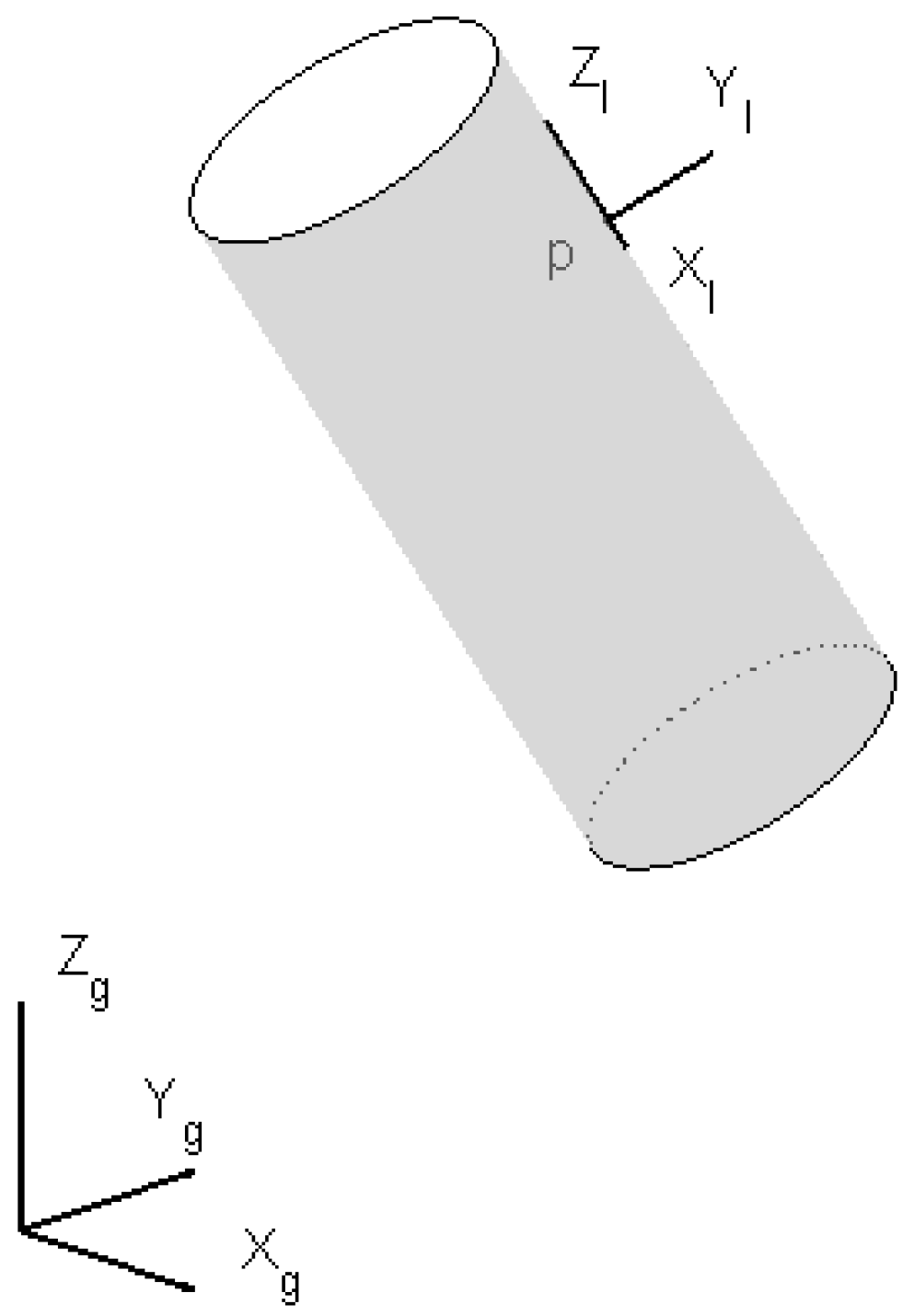
where are the points on the cylinder surface, is a point on the axis, is the direction of the axis of the cylinder with a unit length, and r is the radius. The distance, or the residual, between the laser point and the cylinder surface is . The laser points were weighted to reduce the effect of cross errors, e.g., the points reflected from the branches. The entire stem model was reconstructed in a growing manner. The initial parameters of the model element were the estimations of the previous cylinder. For more details on the robust modeling procedure, please refer to [27].

3.3. DBH Estimation and Location Map for Changed Stems

The DBHs and locations of the harvested stems were automatically estimated using the stem models. The model element at breast height was selected. The diameter and position of the cylinder served as the DBH and the stem location estimation, respectively. Breast height was defined as the point 1.3 m above the ground level; and the ground height was estimated based on the lowest data point around the stem model. The location map for the changed stems was constructed to evaluate the change detection method.

4. Results and Discussion

The changes in forest structure over time were detected using the developed method. The result of the detection on Plot 1 is displayed in Figure 5. Figure 5(a,b) are the TLS data at Time I and Time II, respectively. Figure 5(c) shows the laser points from the harvested stems. Figure 5(d) displays the models of the harvested stems.

Figure 5. The detection in forest structure over time: (a) the TLS data at Time I; (b) the TLS data at Time II; (c) the laser points from the changed stems; (d) the stem models.

Figure 5. The detection in forest structure over time: (a) the TLS data at Time I; (b) the TLS data at Time II; (c) the laser points from the changed stems; (d) the stem models.

The location map of harvested stems was matched with the data reference to evaluate the algorithm. Table 4 summarizes the mapping results. The harvested stems refer to the number of harvested stems in the reference data. The mapped changes represent the number of harvested stems detected from the point cloud using the presented method. Omission is the number of harvested stems not found. Commission is the number of detected harvested stems lacking corresponding references.

In the experiment, five harvested stems were not mapped, which represents the omission error. These trees were partly occluded by other objects and only a small proportion of the stem was included in the data set. The commission errors were those detected changes without correspondences in the references. Two extra changes were detected, and both were harvested stems. They were not included in the reference because of their properties. One stood on the border of the plot, and the other was a dead tree that was not considered in the inventory. Thus, there were no extra detected stems, which had not changed in reality. The overall accuracy of the stem status detection was 96 percent when considering 137 reference trees in the point clouds. The accuracy of the harvested stem detection was 90 percent accounting for 92 percent of the removed basal area.

Table 4. Summary of change detection from the single-scan TLS data.

Plot	1	2	3	4	5
Harvested stems	7	10	13	8	12
Mapped stems	7	8	13	5	12
Omission	0	2	0	3	0
Commission	0	0	1	1	0

Table 4. Summary of change detection from the single-scan TLS data.

Plot	1	2	3	4	5
Harvested stems	7	10	13	8	12
Mapped stems	7	8	13	5	12
Omission	0	2	0	3	0
Commission	0	0	1	1	0

The experiment demonstrated that the proposed method is capable of detecting harvested tree stems if the changed point clouds include this information. To be able to cover close to 100 percent of the changed trees, multi-scan measurements are needed. It is worth noting that the operational cost of multi-scan measurements is higher than that of single-scan measurements. It currently takes 2–4 min for a commercial phase-shift scanner to perform a full field-of-view scan, e.g., 360-by-310 degrees. However, the multi-scan measurement is the only method to map all trees on the dense forest plots. The proposed method can be directly applied to multi-scan measurements without modifications.

The mean bias (bias = estimation − reference) of the DBH estimated for the harvested trees was 0.16 cm and the root mean square error (RMSE) was 1.29 cm, based on 45 mapped stems. If one outlier (due to heavy occlusion) was removed, the mean bias was 0.04 cm and the RMSE was 0.98 cm. (The mean deviation, reference-estimation, was −0.16 cm and −0.04 cm respectively.)

Prior state-of-the-art studies revealed that DBH has been estimated in a sparse forest (212–410 stems/ha) with RMSE of 1.8–3.25 cm using single-scan data and with RMSE of 1.48 cm using multi-scan data [15]. In addition it has been reported that DBH can be derived with RMSE of 3.4–3.74 cm using multi-scan data in a sparse forest (212 stems/ha) [28], and with RMSE 9.17 cm in a sparse urban forest using single-scan data [29]. In a dense forest stand (1,031 stems/ha), the RMSE of the DBH has been reported to be between 1.9 and 3.7 cm [17].

The improved estimation accuracy in this study is attributed to the applied method. In previous research, the DBH has been typically estimated in two-dimensions (2-D) with the points around the DBH height being projected onto the XY plane. Circle fitting or Hough transformation has been used to determine the diameter. In practice, tree stems typically lean towards certain directions. Errors arise from the projection of a stem section onto a 2-D plane. In the present method, each stem section was estimated using a 3-D cylinder model and a robust fitting procedure. The stem direction and its radius were estimated simultaneously. In addition, the entire stem model was constructed. The initial approximation values of the parameters were the results of the previous fitting procedure, which was an advantage of the model fitting.

The method applied here detects changes in the time-series data based on the data and the object basis. In the data-orientated analysis, the approximate changes are detected in the voxel space. The changes are identified by comparing the number of points in voxel units, which is fast and simple. However, the detected changes correspond to various objects on the plot, e.g., the ground and the tree crown. The object-orientated analysis accurately identifies the object subjected to changes by constructing the entire stem model. For example, some stem points may be falsely identified as changed points in the data-orientated analysis because of tree movement caused by the wind. However, it is not possible to construct an entire stem model for such points because the number of points is very limited. In general, object modeling requires far more computation than the comparing operation. The proposed method combines data- and object-orientated analyses. Intensive computation is concentrated on the subset of original points.

The developed method was tested with bi-temporal terrestrial laser scanning data in the detection of harvested trees. The experiment was performed on five forest plots including 137 trees and 50 harvested trees in point clouds. To date, these test sets are among the largest data sets reported for the plot level forest inventory. It is worth noting that it is complicated to arrange change detection studies because it requires the permission of the land owners; however, more extensive data sets are needed in future studies.

The present study also reveals some interesting new potential study topics for further research, e.g., the estimation of decrease in stand volume and biomass in time-series data. The proposed method automatically reconstructs detailed 3-D models of changed tree stems. By applying similar techniques, not only can the volume and biomass changes be monitored after harvesting, but they can also be predicted before the real changes occur. Conventional field measurement methods cannot be used to measure changes in tree volume and biomass accurately or automatically. The technique proposed in this paper emphasizes the possibility of forest managements in a more accurate and precise manner.

Another potential application is the measurement of changes on the permanent sample plots used in national forest inventories (NFIs). In the NFI, permanent sample plots are usually re-measured about every 10 years. Multi-temporal TLS can be considered as having high potential for data collection from the standpoints of growth and biomass models. TLS mensuration provides a relatively speedy technique for acquiring the data required in these model construction processes. The accuracy of multi-temporal TLS measurements in tree-wise growth measurements should be further studied.

It would also be an interesting topic to apply the presented algorithm to different types of forests. The growth environment of forests can be different; thus, stem forms and plot properties between different types of forests may vary. For example, in urban forests, management activities and competition between trees are less intensive compared with managed forests. Thus, trees in urban forests, especially deciduous trees, are likely to have complex stem forms, and the detection of structure changes in such an environment can be challenging. Further studies are needed to explore the applications of multi-temple TLS in different types of forests.

5. Conclusions

This paper presents a fully automated algorithm using bi-temporal terrestrial laser scanning data to detect harvested stems in a typical boreal forest environment. The algorithm was developed based on a 3-D point processing technique and it works for both single- and multi-scan terrestrial laser-scanning measurements. The algorithm was tested on five densely populated managed forest plots. The point clouds totally capture 137 trees, out of which 50 trees had been harvested between terrestrial laser scanning acquisitions. The diameters at breast height of the changed stems were estimated with root-mean-squared-error of 1.29 cm. The overall detection accuracy of the harvested changed stems was 90 percent when using the single-scan approach accounting for 92 percent of the removed basal area. The omissions were occluded stems, where no adequate point cloud has been recorded for these trees, and commissions were dead or border trees, which had not been recorded in the field data. Thus, the developed method found all the changed trees having an adequate point cloud in the changed data. This study demonstrates that the bi-temporal terrestrial laser scanning data can be automatically processed in the detection of tree stem changes on forest plots. The diameters at breast height can be accurately accessed by using the single-scan data. These make it possible to estimate more features of removed trees, as the diameters at breast height are widely used as the basic input in the tree feature estimation. In order to cover close to 100 percent of the changed trees, multi-scan measurements should be employed. Further research is needed to access volume and biomass changes over time based on the detected individual tree stems.

References

1. Lehtonen, A.; Mäkipää, R.; Heikkinen, J.; Sievänen, R.; Liski, J. Biomass expansion factors (BEFs) for Scots pine, Norway spruce and birch according to stand age for boreal forests. Forest Ecol. Manage. 2004, 188, 211–224. [Google Scholar] [CrossRef]
2. Holopainen, M.; Vastaranta, M.; Rasinmäki, J.; Kalliovirta, J.; Mäkinen, A.; Haapanen, R.; Melkas, T.; Yu, X.; Hyyppä, J. Uncertainty in timber assortment estimates predicted from forest inventory data. Eur. J. Forest Res. 2010, 129, 1131–1142. [Google Scholar] [CrossRef]
3. Holopainen, M.; Vastaranta, M.; Kankare, M.; Räty, M.; Vaaja, M.; Liang, X.; Yu, X.; Hyyppä, J.; Hyyppä, H.; Kaasalainen, S.; et al. Biomass Estimation of Individual Trees Using TLS Stem and Crown Diameter Measurements. In Proceedings of ISPRS Workshop Laser Scanning, Calgary, AB, Canada, 29–31 August 2011.
4. Vastaranta, M.; Korpela, I.; Uotila, A.; Hovi, A.; Holopainen, M. Mapping of snow-damaged trees in bi-temporal airborne LiDAR data. Eur. J. Forest Res. 2012, 131, 1217–1228. [Google Scholar] [CrossRef]
5. Yu, X.; Hyyppä, J.; Kaartinen, H.; Maltamo, M. Automatic detection of harvested trees and determination of forest growth using airborne laser scanning. Remote Sens. Environ. 2004, 90, 451–462. [Google Scholar] [CrossRef]
6. Pouliot, D.A.; King, D.J.; Bell, F.W.; Pitt, D.G. Automated tree crown detection and delineation in high-resolution digital camera imagery of coniferous forest regeneration. Remote Sens. Environ. 2002, 82, 322–334. [Google Scholar] [CrossRef]
7. Holmström, H.; Kallur, H.; Ståhl, G. Cost-plus-loss analyses of forest inventory strategies based on kNN-assigned reference sample plot data. Silva Fennica 2003, 37, 381–398. [Google Scholar]
8. Aschoff, T.; Spiecker, H. Algorithms for the automatic detection of trees in laser scanner data. Int. Arch. Photogramm. Remote Sens. Spat. Inform. Sci. 2004, 36, 71–75. [Google Scholar]
9. Thies, M.; Pfeifer, N.; Winterhalder, D.; Gorte, B.G.H. Three-dimensional reconstruction of stems for assessment of taper, sweep and lean based on laser scanning of standing trees. Scand. J. Forest Res. 2004, 6, 571–581. [Google Scholar]
10. Watt, P.J.; Donoghue, D.N.M. Measuring forest structure with terrestrial laser scanning. Int. J. Remote Sens. 2005, 26, 1437–1446. [Google Scholar] [CrossRef]
11. Henning, J.G.; Radtke, P.J. Ground-based laser imaging for assessing three-dimensional forest canopy structure. Photogramm. Eng. Remote Sensing 2006, 72, 1349–1358. [Google Scholar]
12. Henning, J.G.; Radtke, P.J. Detailed stem measurements of standing trees from ground-based scanning lidar. Forest Sci. 2006, 52, 67–80. [Google Scholar]
13. Hopkinson, C.; Chasmer, L.; Young-Pow, C.; Treitz, P. Assessing forest metrics with a ground-based scanning lidar. Can. J. Forest Res. 2004, 34, 573–583. [Google Scholar] [CrossRef]
14. Hosoi, F.; Omasa, K. Factors contributing to accuracy in the estimation of the woody canopy leaf-area-density profile using 3D portable lidar imaging. J. Exp. Bot. 2007, 58, 3464–3473. [Google Scholar]
15. Maas, H.-G.; Bienert, A.; Scheller, S.; Keane, E. Automatic forest inventory parameter determination from terrestrial laser scanner data. Int. J. Remote Sens. 2008, 29, 1579–1593. [Google Scholar] [CrossRef]
16. Lefsky, M.; McHale, M.R. Volume estimates of trees with complex architecture from terrestrial laser scanning. J. Appl. Remote Sens. 2008, 2, 023521. [Google Scholar] [CrossRef]
17. Tansey, K.; Selmes, N.; Anstee, A.; Tate, N.J.; Denniss, A. Estimating tree and stand variables in a Corsican Pine woodland from terrestrial laser scanner data. Int. J. Remote Sens. 2009, 30, 5195–5209. [Google Scholar] [CrossRef]
18. Liang, X.; Litkey, P.; Hyyppä, J.; Kaartinen, H.; Kukko, A.; Holopainen, M. Automatic plot-wise tree location mapping using single-scan terrestrial laser scanning. Photogramm. J. Fin. 2011, 22, 37–48. [Google Scholar]
19. Seidel, D.; Beyer, F.; Hertel, D.; Fleck, S.; Leuschner, C. 3D-laser scanning: A non-destructive method for studying above-ground biomass and growth of juvenile trees. Agr. Forest Meteorol. 2011, 151, 1305–1311. [Google Scholar] [CrossRef]
20. Liang, X.; Hyyppä, J.; Kankare, V.; Holopainen, M. Stem Curve Measurement Using Terrestrial Laser Scanning. In Proceedings of 11th International Conference on LiDAR Applications for Assessing Forest Ecosystems, Hobart, TAS, Australia, 16–20 Ocotober 2011.
21. Zogg, H.-M.; Ingensan, H. Terrestrial laser scanning for deformation monitoring—Load tests on the felsenau viaduct (CH). Int. Arch. Photogramm. Remote Sens. Spat. Inform. Sci. 2008, 37, 555–562. [Google Scholar]
22. Lindenbergh, R.; Pfeifer, N.; Rabbani, T. Accuracy analysis of the Leica HDS3000 and feasibility of tunnel deformation monitoring. Int. Arch. Photogramm. Remote Sens. Spat. Inform. Sci. 2005, 36, 24–29. [Google Scholar]
23. Schneider, D. Terrestrial Laser Scanning for Area Based Deformation Analysis of Towers and Water Damns. In Proceedings of 3rd IAG Symposium of Geodesy for Geotechnical and Structural Engineering and 12th FIG Symposium on Deformation Measurements, Baden, Austria, 22–24 May 2006.
24. Young, A.P.; Olsen, M.J.; Driscoll, N.; Flick, R.E.; Gutierrez, R.; Guaz, R.T.; Johnstone, E.; Kuester, F. Comparison of airborne and terrestrial Lidar estimates of seacliff erosion in southern California. Photogramm. Eng. Remote Sensing 2010, 76, 421–427. [Google Scholar]
25. Resop, J.P.; Hession, W.C. Terrestrial laser scanning for monitoring streambank retreat: Comparison with traditional surveying techniques. J. Hydraul. Eng. 2010, 136, 794–798. [Google Scholar] [CrossRef]
26. Litkey, P.; Puttonen, E.; Liang, X. Comparison of Point Cloud Data Reduction Methods in Single-Scan TLS for Finding Tree Stems in Forest. In Proceedings of 11th International Conference on LiDAR Applications for Assessing Forest Ecosystems, Hobart, TAS, Australia, 16–20 Ocotober 2011.
27. Liang, X.; Litkey, P.; Hyyppä, J.; Kaartinen, H.; Vastaranta, M.; Holopainen, M. Automatic stem mapping using single-scan terrestrial laser scanning. IEEE Trans. Geosci. Remote Sens. 2012, 50, 661–670. [Google Scholar] [CrossRef]
28. Huang, H.; Li, Z.; Gong, P.; Cheng, X.; Clinton, N.; Cao, C.; Ni, W.; Wang, L. Automated methods for measuring DBH and tree heights with a commercial scanning Lidar. Photogramm. Eng. Remote Sensing 2011, 77, 219–227. [Google Scholar]
29. Moskal, M.; Zheng, G. Retrieving forest inventory variables with terrestrial laser scanning (TLS) in urban heterogeneous forest. Remote Sens. 2012, 4, 1–20. [Google Scholar]