Geoprocessing Journey-to-Work Data: Delineating Commuting Regions in Dalarna, Sweden

Abstract

Delineation of commuting regions has always been based on statistical units, often municipalities or wards. However, using these units has certain disadvantages as their land areas differ considerably. Much information is lost in the larger spatial base units and distortions in self-containment values, the main criterion in rule-based delineation procedures, occur. Alternatively, one can start from relatively small standard size units such as hexagons. In this way, much greater detail in spatial patterns is obtained. In this paper, regions are built by means of intrazonal maximization (Intramax) on the basis of hexagons. The use of geoprocessing tools, specifically developed for the processing of commuting data, speeds up processing time considerably. The results of the Intramax analysis are evaluated with travel-to-work area constraints, and comparisons are made with commuting fields, accessibility to employment, commuting flow density and network commuting flow size. From selected steps in the regionalization process, a hierarchy of nested commuting regions emerges, revealing the complexity of commuting patterns.

1. Introduction

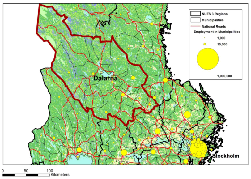
Dalarna is a county in central Sweden comprising of 15 municipalities with a total land area of 28,194 km² and a population of 277,000 in 2010. It is located northwest of Stockholm and has a varied landscape, from mountains in the northern part along the Norwegian border to plains with lakes in the central and southern parts (see Figure 1). The industrial basis of the economy is dominated by paper and pulp, and iron and steel. It is also a popular tourist destination. The largest cities are Borlänge and Falun. Together they contain 28.5% of the county’s population.

For this paper, journey-to-work patterns in Dalarna have been analyzed from different perspectives using geographical information system (GIS) technology and data obtained from a processed subset of the LISA database of Statistics Sweden for the year 2008. This database contains registered places of residence and work. The two registrations are done at different points in time and are not limited to daily commuting, which is a disadvantage. Amcoff [1] has detected a number of errors in the database, related to the inclusion of migration data, weekly commuting and incorrect residential registrations. A small percentage of the records also do not include coordinates and had to be removed from the subset. Despite these shortcomings, the LISA database is a valuable source for spatial analysis. Journey-to-work patterns provide information on important daily movements. To know how large commuting flows are, where they come from and what the relationship is between an employment center and its surroundings can be of great value to businesses recruiting their labor force there. It can also be of value to authorities who define, implement and monitor labor policies, and to transportation planners who study trip patterns.

Figure 1. The location of Dalarna.

Figure 1. The location of Dalarna.

The average size of a municipality in Dalarna is 1,880 km². There are large size differences. The smallest municipality is 574 km² and the largest 6,914 km². A problem generally underestimated in the delineation of commuting regions is the variable size of administrative units, often municipal areas. This causes a distortion in analysis results as the probability of commuting trips with origin as well as destination inside such a unit is higher in larger units [2]. One aspect related to this problem is the aggregation of point-based spatial objects into areal units of variable size, such as municipalities. Another aspect is that self-containment, the main criterion in labor market delineation, is difficult to use with very small base spatial units, as will be explained later. In this way, much commuting information is lost, especially in the larger municipalities. For these reasons, the county has been divided in 1,330 hexagons of 23.4 km² each, with all origins and destinations of the employed population allocated to them. This is possible in a country such as Sweden as population data are available on a fine grid of 0.25 km in urban areas and 1 km in rural areas. A number of hexagon sizes have been tested. With a hexagon size of 23.4 km², most employment centers in the county fit within one hexagon, while a clear differentiation is obtained between employment centers and residential areas.

A critical step in the data processing is the allocation of all individual origins and destinations to hexagons. Individual trips are then bundled into flows. The result is an aggregation from squares to hexagons. Next, commuting flows can be determined by interlinking the hexagon centroids of origins and destinations. External commuting, i.e., flows from and to other counties can be calculated, too. On a county level, there is substantially more out-commuting than in-commuting (see Table 1). As a result, the number of employed residents in the county is much larger than the number of jobs. Internal commuting in the hexagons is 25.6% of employed residents. This is much lower than for municipalities, where it is 71.3%. The origin–destination matrix created for this study only contains flows within hexagons and between hexagons in the county. However, employed resident numbers include external out-commuters, i.e., persons employed outside the county, while job numbers include external in-commuters, i.e., persons living outside the county.

Table 1. Commuting statistics for Dalarna.

Employed Residents	175,130
Jobs	139,297
Internal Commuting	44,914
In-commuting (Including External In-commuting)	94,383
Out-commuting (Including External Out-commuting)	130,216
External In-commuting	8,577
External Out-commuting	44,410

Table 1. Commuting statistics for Dalarna.

Employed Residents	175,130
Jobs	139,297
Internal Commuting	44,914
In-commuting (Including External In-commuting)	94,383
Out-commuting (Including External Out-commuting)	130,216
External In-commuting	8,577
External Out-commuting	44,410

The table indicates that parts of the county, mainly in the south, are integrated into labor markets outside the county. Net in-commuting is equal to net out-commuting, namely 85,806. Adding this figure to internal commuting gives the total number of commuting trips within the county, namely 130,720. Ninety percent of these trips are within a Euclidian distance of 25 km (see Table 2). With a curve factor of 1.2, the road distance is 30 km. Almost two-thirds of all trips are within 10 km Euclidian distance.

Commuting regions or journey-to-work areas can be delineated with different delineation procedures. Cladera and Bergadà [3] distinguish two basic approaches: a rule-based approach that emphasizes attraction experienced by peripheries with respect to employment centers and an approach that emphasizes interaction between different centers. In addition to the general variable administrative unit size problem mentioned earlier, rule-based methods have a drawback that the constraints used in the delineation process are arbitrarily selected [4], whereas a drawback of the interaction-based hierarchical clustering methods is that the configuration of regions created at a specific step in the regionalization is subjectively assessed [4]. Hierarchical clustering cannot guarantee that the demanded maximization of within-region mobility is optimal [5]. Although it is very difficult to find optimal solutions [4], the problem has been addressed by the application of a modularity quality function [4,6] or an evolutionary regionalization algorithm [7].

Contrary to the attempts made to find (near) optimal configurations, the aim of this paper is, using Dalarna as an example, to evaluate different configurations of commuting regions with the Intramax hierarchical clustering method starting from a hexagonal pattern of relatively small base spatial units. In the analysis, travel-to-work area constraints are used to assess these configurations, which are subsequently compared with the commuting patterns found using commuting fields, network accessibility to employment, commuting flow density and network commuting flow size. To support the analysis, use is made of a number of geoprocessing tools, two of them purpose-built, namely the Intramax region builder tool and the commuting field builder tool.

The paper is structured as follows: First, an exposition is given of the Intramax algorithm and the indicators used to assess the results obtained with this algorithm. Next, spatial patterns of residence- and workplace-based self-containment are created. Next, it is shown what values of residence-based self-containment are obtained at different steps in the regionalization process and how the respective configurations compare with spatial patterns obtained with the other indicators. Finally, a judgment is passed on these results with reference to the local labor market area configuration used by Statistics Sweden.

Table 2. Commuting trips within a specific Euclidian distance.

Within (km)	Number of Trips	% of Total
5	44,914	34.4
10	87,935	67.3
15	101,400	77.6
20	111,138	85.0
25	117,159	89.6
30	120,295	92.0

Table 2. Commuting trips within a specific Euclidian distance.

Within (km)	Number of Trips	% of Total
5	44,914	34.4
10	87,935	67.3
15	101,400	77.6
20	111,138	85.0
25	117,159	89.6
30	120,295	92.0

2. Methods

In this paper, the method of hierarchical clustering, using Intramax analysis, is being followed to delineate commuting regions, but avoiding the problem caused by the variable size of base spatial units and using residence-based self-containment and number of employed residents as indicators for the selection of configurations. The constraints used here as a benchmark are the minima of 66.67% self-containment and 3,500 employed residents set for travel-to-work areas (TTWAs) in Great Britain [8]. In TTWAs [9], size and self-containment criteria have been applied together with an interaction function, but a trade-off is used between self-containment and resident employed population. A TTWA has a large resident employed population and a high self-containment value. The size constraint used in this analysis is very low. In the TTWA delineation for Great Britain, a range between 3,500 and 25,000 employed residents is used now [10], whereas for Germany a constraint of 50,000 is seen as acceptable [11]. TTWAs are partly rule-based since the regionalization process is always started at employment centers that meet the self-containment criterion. However, self-containment and size constraints have been adapted to changed circumstances through the years [8].

2.1. Intramax Analysis

Interaction functions are used as objective functions in hierarchical clustering algorithms. One such algorithm is intrazonal maximization or Intramax. This algorithm identifies functional regions by hierarchically aggregating spatial base units in order to create homogeneous clusters. Intramax is an agglomerative or bottom-up clustering algorithm that starts with as many clusters as there are base units. Clusters are then successively merged until finally one cluster is left. A contiguity constraint is thereby taken into account [12]. In this context, Masser and Brown [13] define a functional region as an area that is delimited by maximizing the proportion of total interaction occurring within the aggregation of base units that form the diagonal elements of the origin–destination matrix, thereby minimizing “the proportion of cross-boundary movements in the system as a whole.”

Intramax analysis is a stepwise procedure using an objective function, where with N spatial units, after N-1 steps, all spatial units are aggregated into a single region. All interaction is then intrazonal. The procedure can be visualized by means of a dendrogram. “The objective of the Intramax procedure is to maximize the proportion within the group interaction at each stage of the grouping process, while taking into account the variations in the row and column totals of the matrix” [13]. Each pair of regions is investigated at each step in the regionalization process. Two regions are merged for which the objective function has been maximized. The objective function of this algorithm is:

(1)

where T_ij = interaction between origin region i and destination region j

(2)

where O_i = total outflow from region i

(3)

where D_j = total inflow into region j

The objective function can only be calculated for D_j > 0 and for O_i > 0 [12].

Intramax analysis is part of the spatial analysis software package Flowmap, developed at Utrecht University [12]. The input consists of an origin file, a destination file and a flow file providing for each OD-pair its flow size, i.e., number of movements. Output of Intramax analysis, besides a dendrogram, is a fusion report, showing the aggregation history and two tables that are built while processing the Intramax fusion report. For each base unit, the first table shows the region that this unit belongs to at a specified step. By joining this table with the polygon file of the base units, regional divisions for a step can be shown on a map by dissolving on the field of this step. The second table shows the flows within and between regions.

Due to the inclusion of the Intramax algorithm in Flowmap, it has been widely used for the delineation of labor markets and commuting regions. The use of the dBase exchange format facilitates coupling with desktop GIS software. Therefore, analysis results can be immediately visualized and evaluated at selected steps in the regionalization process. It has been used to identify travel-to-work areas in Ireland by Meredith et al. [14]. The Centre of Full Employment and Equity (CofFEE) in Australia has used the algorithm for the delineation of CofFEE functional economic areas for that country [15]. Krygsman et al. [16] have used it to delineate functional transport regions in South Africa. It has been used for the delimitation of functional regions in England, Wales and Scotland by Feldman et al. [17], in Newfoundland and Labrador (Canada) in a research project on functional regions [18], in Switzerland by Killer and Axhausen [19] and in Slovenia by Drobne and Bogataj [20].

2.2. Self-Containment

An area receives flows from outside its borders, i.e., has a certain amount of in-commuting, and produces flows that go to other areas, i.e., a certain amount of out-commuting. Size criteria often used in commuting studies are residents employed locally (REL), resident-employed population (REP) and day-employed population (DEP). REL is the population working within the area where it resides, which is equal to internal commuting. REP is the population working within or outside the area where it resides, which is equal to internal commuting plus out-commuting. DEP is the population working within the area or number of jobs, which is equal to internal commuting plus in-commuting.

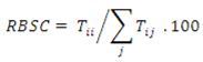
Self-containment is the most important criterion for the selection of employment foci in rule-based delineation procedures, but it can also be used to test functional regions with regard to commuting flows. It refers to the ability of a region or zone to provide employment to its own residents, whereby a distinction is often made between residence-based or supply-side self-containment (RBSC) and workplace-based or demand-side self-containment (WBSC) [21]. RBSC is the share of residents employed within a zone, i.e., internal commuting divided by the number of employed residents, expressed as a percentage:

(4)

where T_ii = internal flow in zone i, T_ij = flow from zone i to zone j, and ∑_j T_ij = total outflow from zone i to zone j (including internal flows).

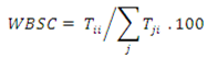
WBSC is the share of jobs inside a zone occupied by residents of this zone, i.e., internal commuting divided by the number of jobs, expressed as a percentage:

(5)

where T_ii = internal flow in zone i, T_ji = flow from zone j to zone i, and ∑_j T_ji = total inflow from zone j to zone i (including internal flows).

2.3. Commuting Fields

From the point of view of the single employment center and looking at one-way flows, one can delineate a commuting region by determining the orientation of in-commuters to this employment center. A classic approach is to consider employment centers as central places, having a surplus of jobs in order to serve their hinterlands. Commuting regions are then nodal regions with a core and periphery. Smolin [22] has delineated commuting regions in central Ohio based on this approach. He called these regions commuting fields in order to indicate that he had obtained zones of influence proportional to the percentage of commuters in other nodes that are oriented at the core of the commuting field. He allowed these regions to overlap each other by fixing the boundary of the commuting field at a relatively low percentage. Nonoverlapping commuting regions can be created by finding the “influence divide” between nodes, thereby delineating, what Smolin called, commuting hinterlands.

2.4. Accessibility to Employment

Accessibility can be measured for a specific destination, but also for all destinations together. Accessibility to an employment center is often shown by means of drive time contours. Voronoi drive time isochrones provide a general view of the time it will take to reach an employment center from its surroundings. It is necessary to set average speeds for each road type. Drive times are indicated by polygons, each related to a specific time period. Overall accessibility can be measured in different ways. One approach is to measure potential accessibility. With the floating catchment area (FCA) method, the catchment area is a distance circle or travel time zone around each resident or demand location, i.e., the centroid of an origin hexagon. A job-residents or supply-to-demand ratio measures accessibility to jobs within the catchment area. The catchment area floats from one resident location to another and determines accessibility to jobs for all resident locations. In the two-step floating catchment area (2SFCA) method, the process of floating catchment is done twice: once on job or supply locations (destinations), once on demand locations (origins) [23].

The procedure for 2SFCA is as follows:

• Choose threshold distance or travel time d₀ from supply location j to determine the catchment area
• Search for each supply location j all demand locations k that are within catchment area j
• Calculate supply-to-demand ratio R_j within the catchment area:

  (6)

where S_j = supply at location j, and D_k = demand at location k

• Search for each demand location i all supply locations j that are within catchment area i
• Sum up R_j at those locations to obtain accessibility A_i at demand location i:

  (7)

2.5. Commuting Flow Density and Network Commuting Flow Size

The line density tool of ArcGIS is used to calculate the density of commuting flows. This tool calculates the density of desire lines for raster cells taking account of flow size. A distance circle is drawn around each raster cell using a specific search radius. The length of the portion of each desire line that falls within the circle is multiplied with its flow size. The total of the multiplications is then divided by the circle’s area to obtain the density of a cell. As in a real situation trips flow on networks, commuting flows are assigned to the major road network in Dalarna using a shortest-path algorithm.

3. Analysis

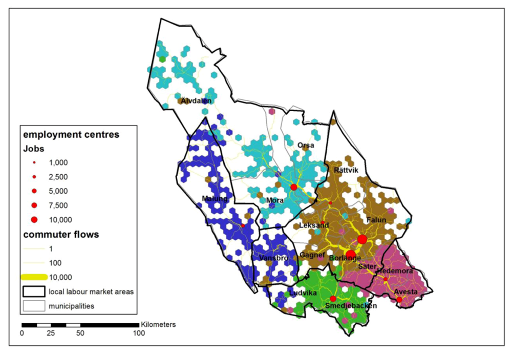
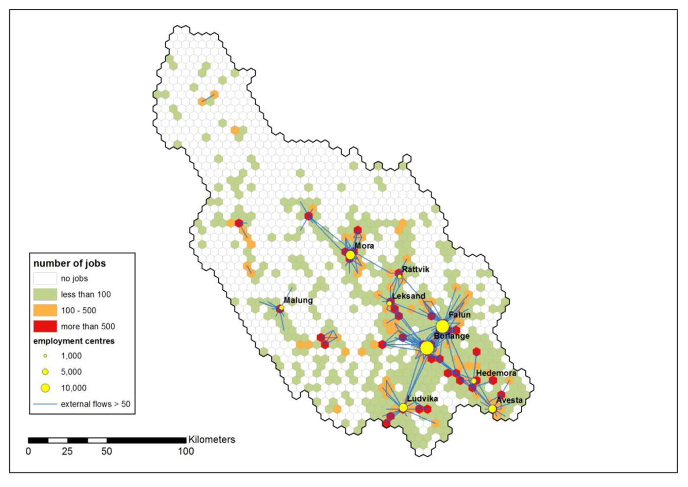
For part of the analysis, nine centers have been selected as major employment centers. Such a center has a core hexagon with 2,000 or more jobs and adjacent hexagons with 1,000 or more jobs. These centers together have 94,402 jobs, which is 67.8% of the total number of jobs in the county. A clear three-level hierarchy exists (see Table 3). There are two large centers, Borlänge and Falun (between 24,000 and 28,000 jobs), three medium centers, Mora, Ludvika and Avesta (between 8,000 and 11,000 jobs) and four small centers, Hedemora, Leksand, Malung and Rättvik (between 2,000 and 4,000 jobs). The day-employed population is very concentrated. 91.7% of the base spatial units have less than 100 jobs or no jobs at all (see Figure 2).

Figure 2. Number of jobs and major employment centers and external flows.

Figure 2. Number of jobs and major employment centers and external flows.

Table 3. Major employment centers.

Employment Center	Number of Jobs
Avesta	8,621
Borlänge	27,477
Falun	24,660
Hedemora	3,920
Leksand	3,520
Ludvika	9,694
Malung	3,149
Mora	10,832
Rättvik	2,529
Total	94,402

Table 3. Major employment centers.

Employment Center	Number of Jobs
Avesta	8,621
Borlänge	27,477
Falun	24,660
Hedemora	3,920
Leksand	3,520
Ludvika	9,694
Malung	3,149
Mora	10,832
Rättvik	2,529
Total	94,402

3.1. Self-Containment

Self-containment has been calculated for 466 hexagons. These are the hexagons that contain resident-employed population as well as day-employed population. A comparison has been made between municipalities and hexagons in Dalarna. Residence-based self-containment of hexagons is substantially smaller and has more variation (see Table 4).

Table 4. Residence-based and workplace-based self-containment in municipalities and hexagons.

Self-Containment	Residence-Based (%)		Work-Place Based (%)
Method	Municipalities	Hexagons	Municipalities	Hexagons
Mean	73.3	19.3	77.9	59.6
Confidence Level (95.0%)	7.583	1.668	2.938	2.812
St. Dev.	13.7	18.3	1.4	30.9
10%	50.1	5.9	73.0	20.1
25%	67.0	8.7	76.2	33.3
50% (Median)	77.8	13.3	78.1	55.1
75%	82.2	23.5	79.6	100.0
90%	84.2	40.2	86.6	100.0

Table 4. Residence-based and workplace-based self-containment in municipalities and hexagons.

Self-Containment	Residence-Based (%)		Work-Place Based (%)
Method	Municipalities	Hexagons	Municipalities	Hexagons
Mean	73.3	19.3	77.9	59.6
Confidence Level (95.0%)	7.583	1.668	2.938	2.812
St. Dev.	13.7	18.3	1.4	30.9
10%	50.1	5.9	73.0	20.1
25%	67.0	8.7	76.2	33.3
50% (Median)	77.8	13.3	78.1	55.1
75%	82.2	23.5	79.6	100.0
90%	84.2	40.2	86.6	100.0

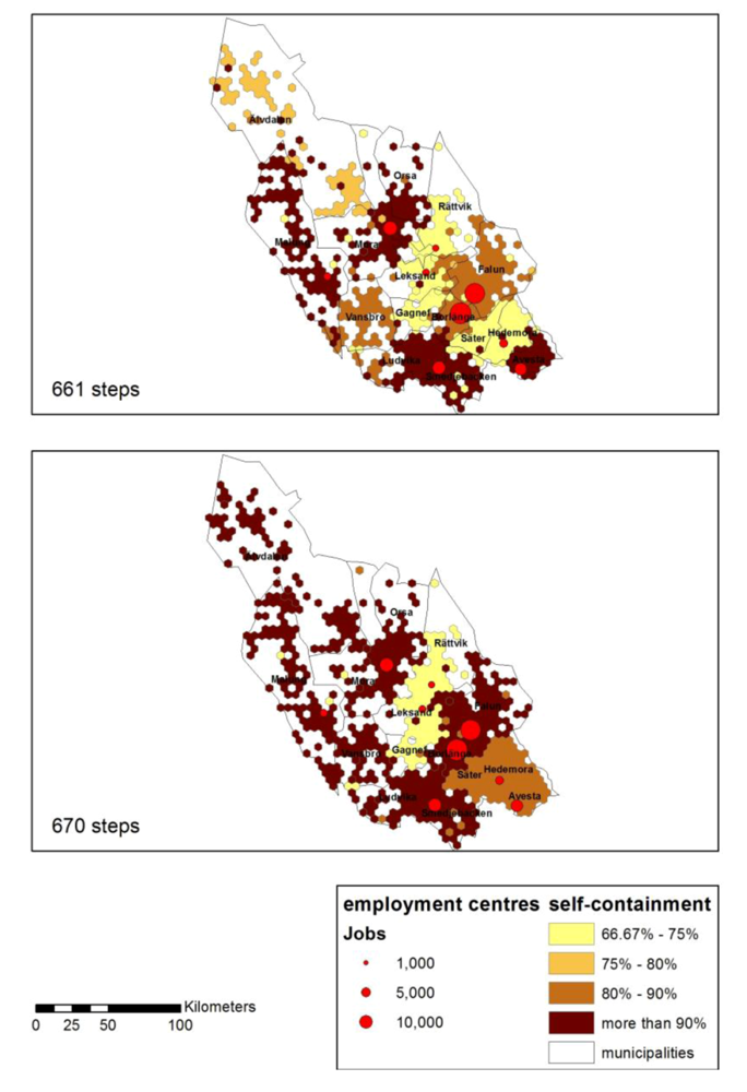
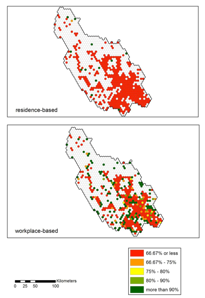
The preponderant low residence-based self-containment of hexagons (see Figure 3) is caused by the small size of the base spatial units. With reference to the base spatial units used in this study, the radius of a circle with an area of 23.4 km² is 2.7 km. The radius of a circle representing the average municipal area in the province is 24.5 km. With 34% of all commuting within 5 km and 90% within 25 km (see Table 2), the reason for this low figure is clear. There are relatively few internal movements as employed residents mainly work elsewhere. In the case of workplace-based self-containment, levels are generally higher as most base spatial units have a small day-employed population.

Figure 3. Residence-based and workplace-based self-containment.

Figure 3. Residence-based and workplace-based self-containment.

Generally, the larger a municipal area, the larger self-containment is. In southern Sweden, a strong positive correlation has been found between municipal land area and both types of self-containment. Coombes and Bond [8] have also found that the larger travel-to-work areas (TTWAs) they delineated in UK tend to have higher self-containment levels. Differences between residence-based and workplace-based self-containment are relatively small. However, if very small base spatial units are used, as in this analysis, these differences become so large that it is not appropriate to use them as selection criteria for employment foci as has been the case with TTWAs.

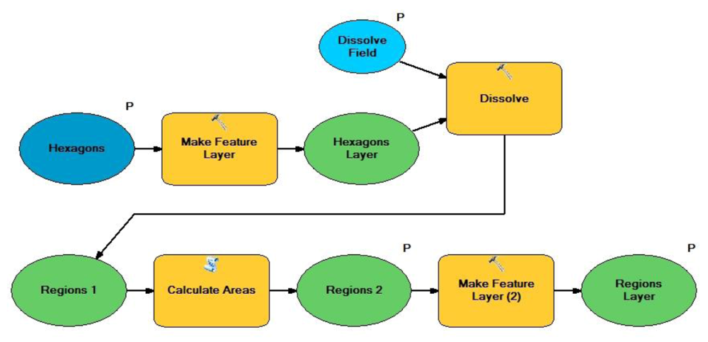
3.2. Intramax Analysis

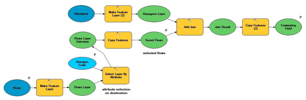
Commuting regions were created with the Intramax algorithm on the basis of commuting trips. Tables were produced after processing the fusion report to obtain region maps for a number of fusion steps in the algorithm. The output of the Intramax analysis was then used as input in a geoprocessing model, created with ArcGIS ModelBuilder [24], that produced a map of commuting regions related to a specific fusion step (see Figure 4).

Figure 4. Intramax region builder tool.

Figure 4. Intramax region builder tool.

To start Intramax analysis in Flowmap, one needs a table that contains the coordinates of the centroids of all hexagons and a flow table that contains the scores for each OD pair. The fusion report shows the increases in cumulative intrazonal interaction while the number of regions is decreasing.

The question arises what step must be chosen to delimit the functional regions. This decision is judgmental. “The Intramax procedure does not include an objective basis for determining the number of market areas. The choice of an appropriate number of markets is at the discretion of the user” [25]. To overcome this problem, Mitchell et al. [15] propose the identification of breaking points in the fusion report “where significant increases in the cumulative intrazonal interaction occur as a result of a fusion”. Breaking points have been detected at steps 642, 645, 647, 657, 669 and 671. At step 642 the number of regions is 25, with 66.7% of trips internal. Table 5 shows the differences between a number of steps with regard to percentage internal commuting and number of functional regions created. The number of regions decreases with every further step.

Table 5. Intramax analysis results at selected steps.

Step	% Internal	Number of Regions
642	66.7	25
645	71.5	22
647	75.6	20
657	79.8	14
661	82.1	11
669	84.4	7
670	89.3	6
671	92.6	5

Table 5. Intramax analysis results at selected steps.

Step	% Internal	Number of Regions
642	66.7	25
645	71.5	22
647	75.6	20
657	79.8	14
661	82.1	11
669	84.4	7
670	89.3	6
671	92.6	5

3.3. Applying TTWA Constraints

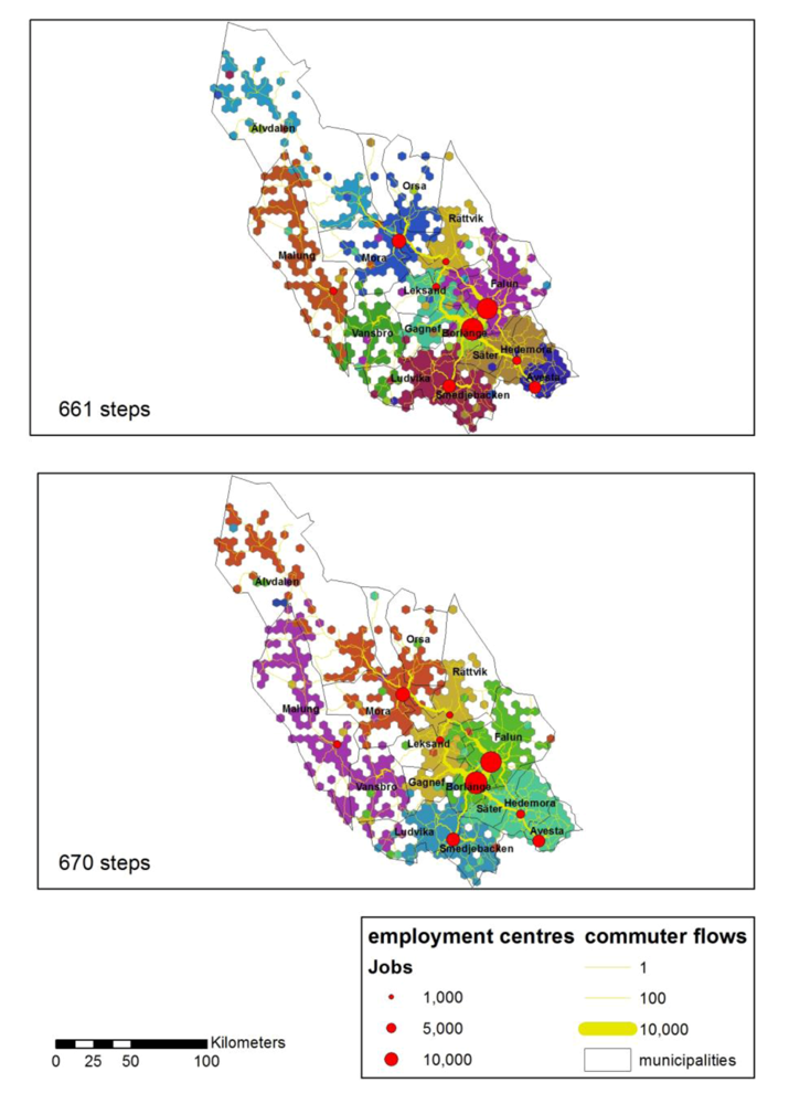
At step 661, very small regions are merged with other regions, resulting in a stable pattern of 11 regions that do not differ substantially in size (see Figure 5). All these regions meet the TTWA self-containment constraint (see Table 6 and Figure 6). However, two regions, Älvdalen and Vansbro, do not have major employment centers. Vansbro is the only region that does not meet the TTWA size constraint of 3,500.

Figure 5. Intramax analysis results at steps 661 (11 regions) and 670 (six regions).

Figure 5. Intramax analysis results at steps 661 (11 regions) and 670 (six regions).

At step 670, six regions are left. All these regions have one or two major employment centers. Self-containment levels are now considerably higher, with four regions having levels above 90%, one region above 80% and one above 70% (see Table 7 and Figure 6). All regions meet the TTWA size constraint. At step 671, five regions are left. The Leksand-Gagnef-Rättvik region, which had a relatively low self-containment level of 73% in the previous step, now has merged with the Borlänge-Falun region (see Table 8).

Table 6. Net residence-based self-containment at step 661.

Region	Internal	Total	% Internal
Älvdalen	2,774	3,502	79.21
Avesta	9,221	10.189	90.40
Borlänge	18,592	23,161	80.27
Falun	21,932	26,558	82.58
Hedemora-Säter	9,035	12,951	69.76
Leksand-Gagnef	7,752	11,329	68.43
Ludvika-Smedjebacken	15,017	16,359	91.80
Malung	4,853	5,223	92.92
Mora-Orsa	12,001	13,129	91.41
Rättvik	3,322	4,909	67.67
Vansbro	2,806	3,375	83.14

Table 6. Net residence-based self-containment at step 661.

Region	Internal	Total	% Internal
Älvdalen	2,774	3,502	79.21
Avesta	9,221	10.189	90.40
Borlänge	18,592	23,161	80.27
Falun	21,932	26,558	82.58
Hedemora-Säter	9,035	12,951	69.76
Leksand-Gagnef	7,752	11,329	68.43
Ludvika-Smedjebacken	15,017	16,359	91.80
Malung	4,853	5,223	92.92
Mora-Orsa	12,001	13,129	91.41
Rättvik	3,322	4,909	67.67
Vansbro	2,806	3,375	83.14

Figure 6. Residence-based self-containment at steps 661 (11 regions) and 670 (six regions).

Figure 6. Residence-based self-containment at steps 661 (11 regions) and 670 (six regions).

Table 7. Net residence-based self-containment at step 670.

Region	Internal	Total	% Internal
Avesta-Hedemora-Säter	19,455	23,140	84.08
Borlänge-Falun	46,953	49,730	94.42
Leksand-Gagnef-Rättvik	11,846	16,238	72.95
Ludvika-Smedjebacken	15,025	16,370	91.78
Malung-Vansbro	7,868	8,598	91.51
Mora-Orsa-Älvdalen	15,571	16,631	93.63

Table 7. Net residence-based self-containment at step 670.

Region	Internal	Total	% Internal
Avesta-Hedemora-Säter	19,455	23,140	84.08
Borlänge-Falun	46,953	49,730	94.42
Leksand-Gagnef-Rättvik	11,846	16,238	72.95
Ludvika-Smedjebacken	15,025	16,370	91.78
Malung-Vansbro	7,868	8,598	91.51
Mora-Orsa-Älvdalen	15,571	16,631	93.63

Table 8. Net residence-based self-containment at step 671.

Region	Internal	Total	% Internal
Avesta-Hedemora-Säter	19,455	23,140	84.08
Borlänge-Falun-Leksand-Gagnef-Rättvik	63,068	65,968	95.60
Ludvika-Smedjebacken	15,025	16,370	91.78
Malung-Vansbro	7,868	8,598	91.51
Mora-Orsa-Älvdalen	15,571	16,631	93.63

Table 8. Net residence-based self-containment at step 671.

Region	Internal	Total	% Internal
Avesta-Hedemora-Säter	19,455	23,140	84.08
Borlänge-Falun-Leksand-Gagnef-Rättvik	63,068	65,968	95.60
Ludvika-Smedjebacken	15,025	16,370	91.78
Malung-Vansbro	7,868	8,598	91.51
Mora-Orsa-Älvdalen	15,571	16,631	93.63

3.4. Commuting Fields

Commuting fields can be constructed in a number of steps using a number of techniques and tools available in ArcMap. The most time-consuming steps have been included in a geoprocessing model using ArcGIS ModelBuilder [24] in order to calculate the commuting field of an employment center (see Figure 7).

The major employment centers of Dalarna consist of single or multiple hexagons. The commuting field builder tool can build a detailed pattern of commuters’ orientation to these centers. In principle, each hexagon of which a percentage of its resident employed population commutes to the selected employment center, i.e., its core, is part of the commuting field. However, a limit of 5% has been applied to be able to delineate it. 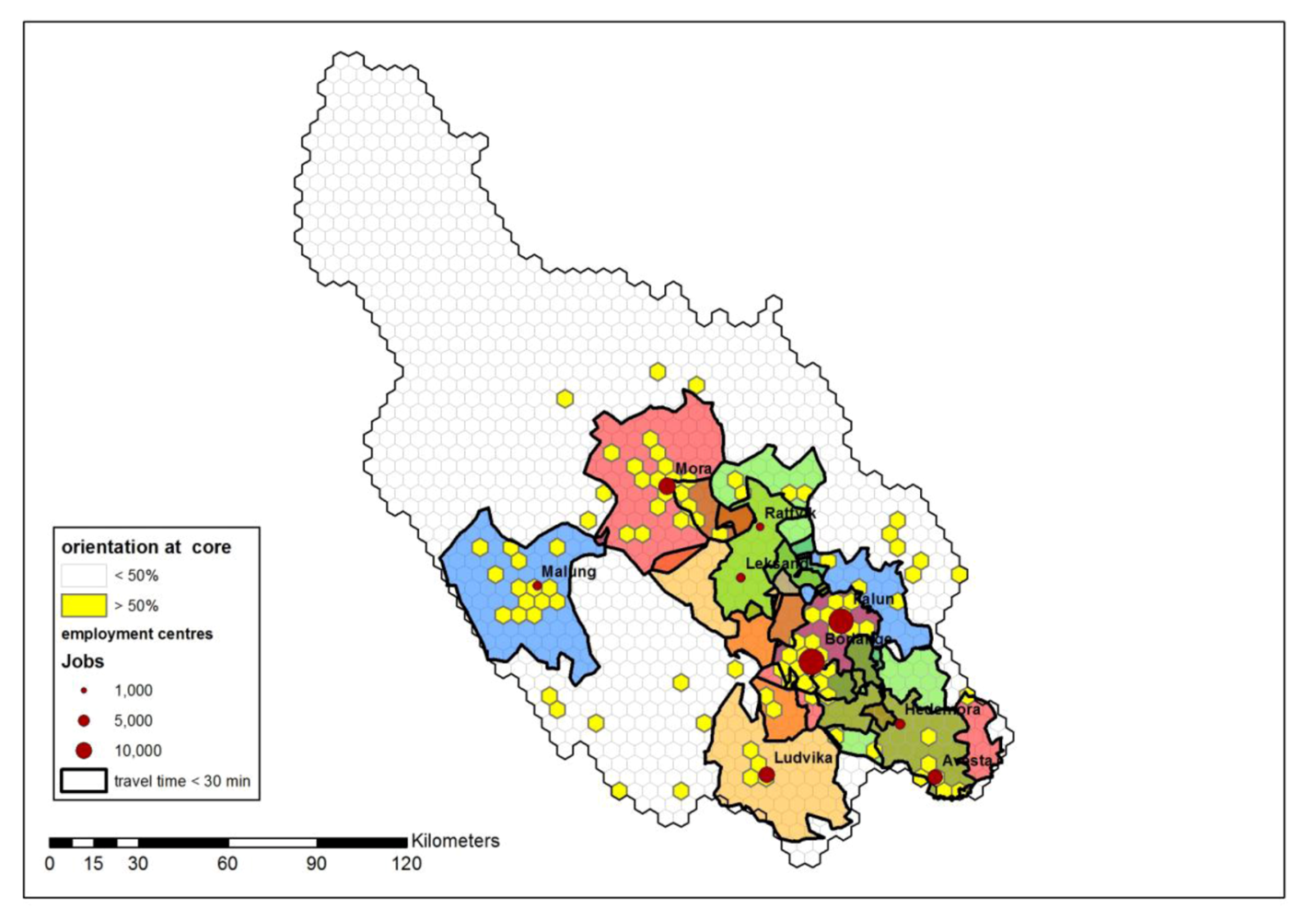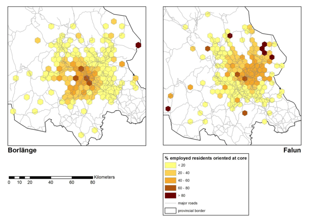Figure 8 shows the (overlapping) commuting fields of the Borlänge and Falun cores with the magnitude of orientation from their peripheries. According to Smolin [22], 50% orientation is a critical magnitude. This is shown in Figure 9 for all major employment centers. Separate clusters attached to a core have been obtained in this way for Borlänge, Falun, Malung, Ludvika, Mora and Avesta.

Figure 7. Commuting field builder tool.

Figure 7. Commuting field builder tool.

Figure 8. Commuting fields of Borlänge and Falun.

Figure 8. Commuting fields of Borlänge and Falun.

Figure 9. Commuting fields and 30 min travel time areas.

Figure 9. Commuting fields and 30 min travel time areas.

3.5. Network Accessibility to Employment

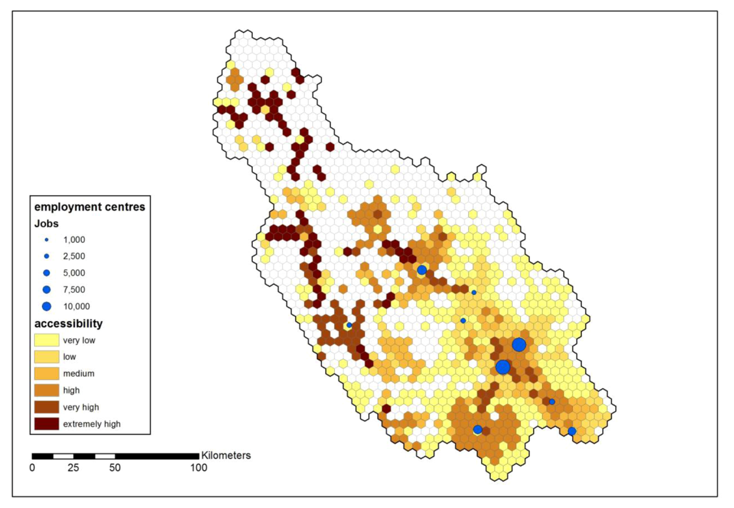
Potential accessibility to employment has been measured with the two-step floating catchment area (2SFCA) method. It gives an indication how labor markets could further develop. Using a 30-min travel time catchment area, thereby covering the vast majority of commuting trips, Figure 10 shows clusters of high accessibility around Älvdalen, Mora, Borlänge-Falun, Ludvika and Hedemora. Areas of very high potential accessibility to extremely high potential accessibility are found along the main roads in the northwestern part of the province and between the high accessibility clusters of Älvdalen and Mora. The area around the main road between Borlänge and Ludvika also has a very high potential accessibility.

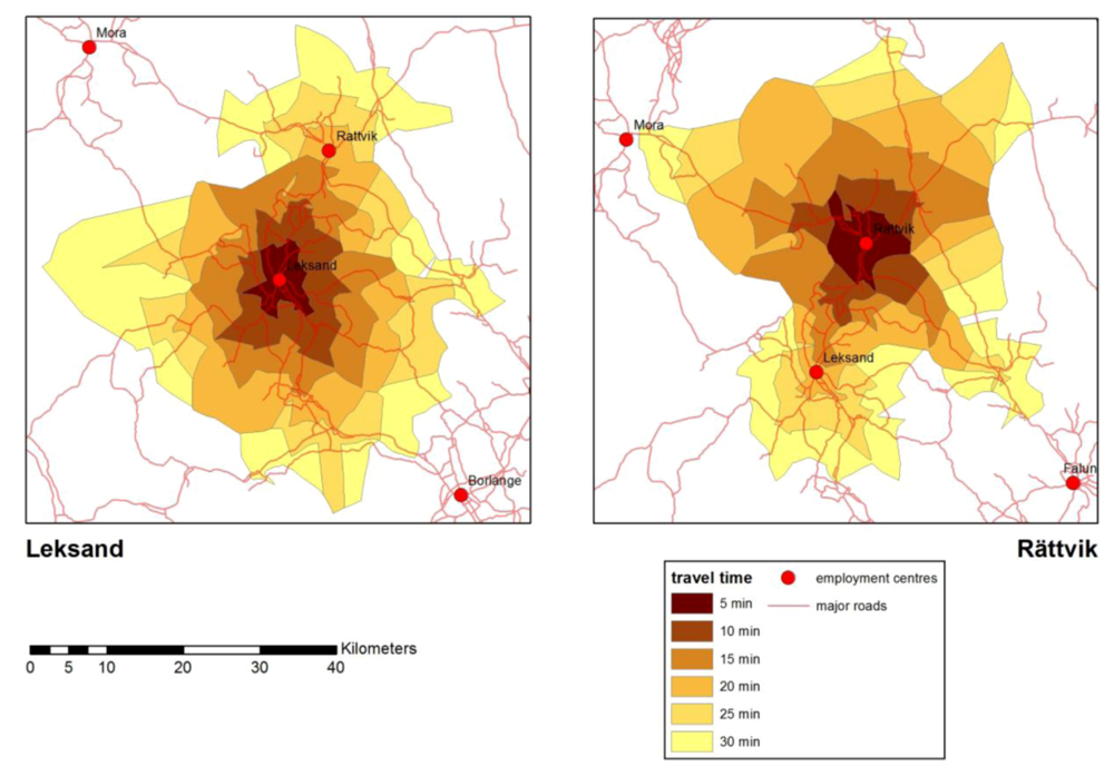
Accessibility to a single employment center has been measured with Voronoi drive time isochrones. Figure 11 shows the 5-min road travel time contours for Leksand and Rättvik to a maximum of 30 min. This method can also be used to determine the amount of overlap between employment centers. The 30-minute travel time areas of Leksand and Rättvik clearly overlap. Similar overlaps have been found between Borlänge and Falun and between Avesta and Hedemora (see Figure 9). Such overlaps are not only an indication of interdependency of employment centers, but they also show that workers can easily switch employment without changing residence.

Figure 10. Network accessibility to employment (30 min travel time on road network).

Figure 10. Network accessibility to employment (30 min travel time on road network).

Figure 11. Voronoi drive time isochrones for Leksand and Rättvik.

Figure 11. Voronoi drive time isochrones for Leksand and Rättvik.

Figure 12. Commuter flows on road network and line density.

Figure 12. Commuter flows on road network and line density.

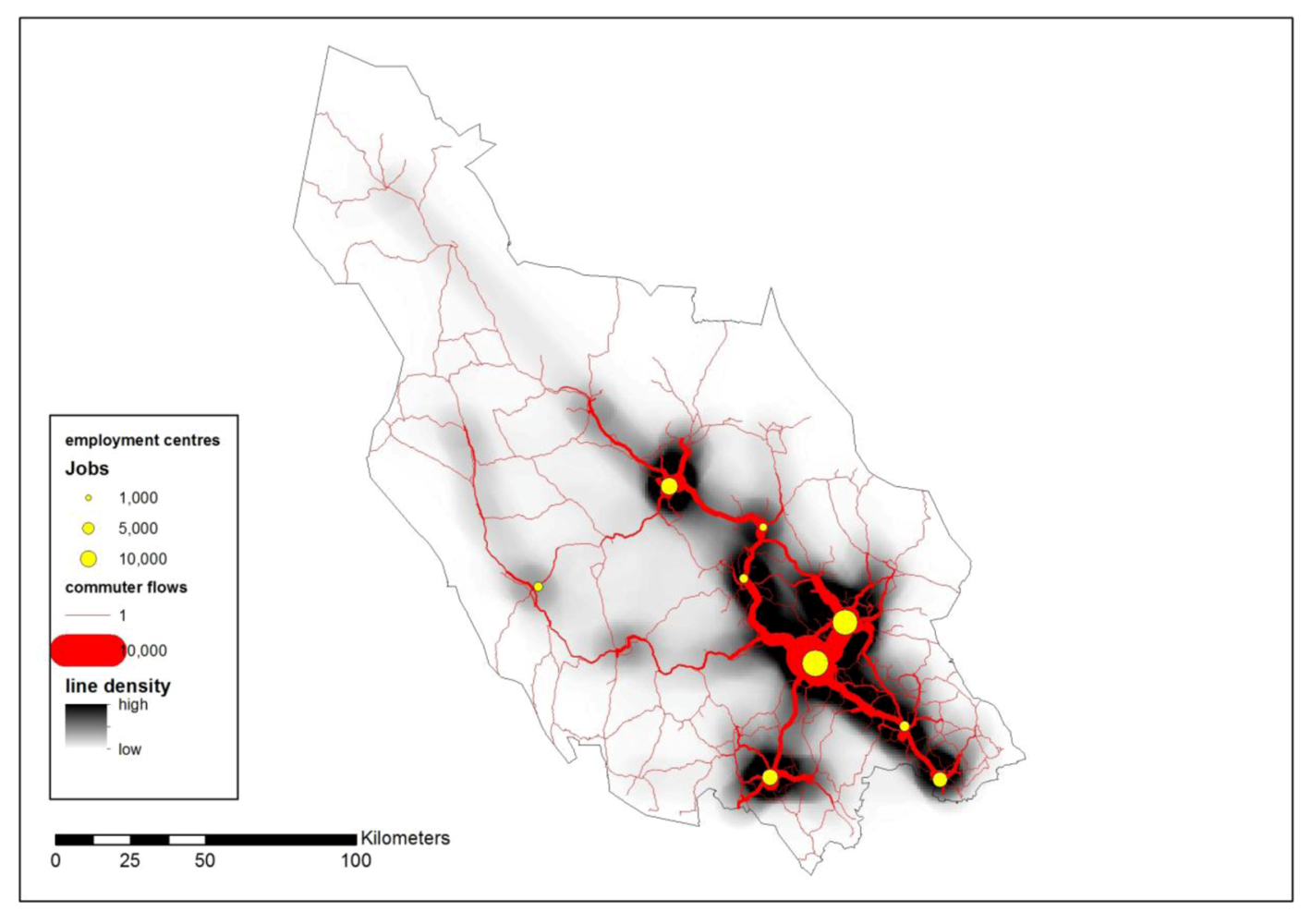
3.6. Commuting Flow Density and Network Commuting Flow Size

Commuting flow size along the road network has been determined using the shortest travel times between origins and destinations. The largest flows occur between Borlänge and Falun, on the roads leading northwest and southeast from Borlänge, northwest and northeast from Falun and northeast, and northeast from Mora and Avesta (see Figure 12). From Ludvika, there are substantial flows in different directions. Large flows coincide with high line density, as calculated with the line density tool.

4. Conclusion

Self-containment as a criterion for delineation has to be used carefully. It has been shown that with small spatial base units, large differences occur between residence-based self-containment and workplace-based self-containment. Therefore, these criteria cannot be used for the selection of employment foci. However, as regionalization proceeds, both types of self-containment will become useful in the assessment of the regions created at different steps in the Intramax analysis.

Fusion results have been obtained for a number of steps. Three of them, suitable candidates for selection as commuting region delineation, have been further investigated. As a result, three levels of commuting regions are proposed: a lower level of 11 Intramax regions with 82.1% internal flows (at step 661), a medium level of six Intramax regions with 89.3% internal flows (at step 670) and a higher level of five Intramax regions with 92.6% internal flows (at step 671). All regions meet the TTWA self-containment constraint at both levels. One Intramax region at the lower level, Vansbro, does not meet the TTWA employment size constraint. This region, which is a local labor market area (LLMA) as delineated by Statistics Sweden [26], has been merged with the Malung region on the medium level (see Figure 5). On the latter level, the Falun region has been merged with the Borlänge region, the Rättvik region with the Leksand-Gagnef region, the Älvdalen region with the Mora-Orsa region and the Hedemora-Säter region with the Avesta region (see Figure 5). On the higher level, the Leksand-Gagnef-Rättvik region has been merged with the Borlänge-Falun region (see Figure 13).

There are strong bonds between the two largest employment centers, Borlänge and Falun. Their commuting fields as well as travel time areas overlap each other and there is a very strong commuting flow between them. The combined region of these centers is also an area of high potential accessibility to very high potential accessibility. The LLMA includes the Leksand-Gagnef-Rättvik region, although the travel time areas of Leksand-Rättvik and Borlänge-Falun do not overlap. The orientation from this region to Borlänge and Falun is also quite low. The Leksand-Gagnef-Rättvik region, which meets the TTWA constraints, is a special case as their relatively small employment centers do not function as cores for a commuting field. This region, situated east of Lake Siljan, contains a number of interrelated settlements that do not differ much in size. Potential accessibility is low. Avesta and Hedemora-Säter form one Intramax region and also a LLMA. However, the Intramax region stretches further to the west. The same applies to the Malung-Vansbro Intramax region, which occupies the most western part of the Ludvika LLMA. This part is outside the Ludvika travel time area, but some of the hexagons there have a relatively strong orientation to Ludvika.

Figure 13. Intramax analysis result at step 671 (five regions) compared with local labor market areas.

Figure 13. Intramax analysis result at step 671 (five regions) compared with local labor market areas.

These differences show that a delineation using hexagons provides much more detail than the municipalities offer. A distinction can also be made between inhabited and uninhabited areas. They also show that a 100% agreement on the borders of commuting areas is not possible.

For the steps of the lower and medium level, Intramax analysis produces more regions than the rule-based method used by Statistics Sweden to delineate LLMAs [19]. At the higher level step, there is a remarkable similarity between the Intramax delineation and the LLMA delineation (see Figure 13). However, the Vansbro LLMA only appears as an Intramax region at the lower level. The latter can be explained by the rule used in the LLMA delineation that a municipality is selected as starting point in the regionalization process if less than 20% of the resident-employed population commutes to other municipalities while the largest commuting flow to any other municipality is less than 7.5% [19]. This allows the selection of relatively small employment centers. It is possible to go to an even higher level, when at step 672 the Avesta-Hedemora-Säter region is merged with the Borlänge-Falun-Leksand-Gagnef-Rättvik region, creating a super-region that remarkably coincides with the line density cluster in this area (see Figure 12). However, the necessity of this additional level can be questioned as the Avesta-Hedemora-Säter region already has a relatively high self-containment level at step 671.

Small hexagons as base spatial units, while excluding uninhabited areas, result in detailed delineations. However, as self-containment cannot be used as a criterion for the selection of employment centers as starting points in the regionalization process, neither the rule-based method for LLMAs nor the hybrid method used for TTWAs are options. For a regionalization process that starts from such small spatial base units, an interaction-based method such as Intramax analysis is very suitable. Intramax analysis also allows delineation of commuting regions at different levels, resulting, in this case, in a three-level or even four-level commuting region hierarchy using the concept of nesting, with each order of the hierarchy fitting in the next higher order [27]. Delineation levels can then subsequently be evaluated using TTWA criteria as well as accessibility and density measures and spheres of influence determined by GIS methods, allowing a critical assessment of results. Another advantage of using these small hexagons is that borders of commuting regions turn out to be fuzzy (see Figure 5 and Figure 13), indicating, to some extent, the incidence of nondaily commuting.