Identifying Urban Wetlands through Remote Sensing Scene Classification Using Deep Learning: A Case Study of Shenzhen, China

Abstract

Urban wetlands provide cities with unique and valuable ecosystem services but are under great degradation pressure. Correctly identifying urban wetlands from remote sensing images is fundamental for developing appropriate management and protection plans. To overcome the semantic limitations of traditional pixel-level urban wetland classification techniques, we proposed an urban wetland identification framework based on an advanced scene-level classification scheme. First, the Sentinel-2 high-resolution multispectral image of Shenzhen was segmented into 320 m × 320 m square patches to generate sample datasets for classification. Next, twelve typical convolutional neural network (CNN) models were transformed for the comparison experiments. Finally, the model with the best performance was used to classify the wetland scenes in Shenzhen, and pattern and composition analyses were also implemented in the classification results. We found that the DenseNet121 model performed best in classifying urban wetland scenes, with overall accuracy (OA) and kappa values reaching 0.89 and 0.86, respectively. The analysis results revealed that the wetland scene in Shenzhen is generally balanced in the east–west direction. Among the wetland scenes, coastal open waters accounted for a relatively high proportion and showed an obvious southward pattern. The remaining swamp, marsh, tidal flat, and pond areas were scattered, accounting for only 4.64% of the total area of Shenzhen. For scattered and dynamic urban wetlands, we are the first to achieve scene-level classification with satisfactory results, thus providing a clearer and easier-to-understand reference for management and protection, which is of great significance for promoting harmony between humanity and ecosystems in cities.

1. Introduction

Humanity is increasingly urban but continues to depend on nature for its survival [1]. As a result, many wetlands may remain in urban areas, both as remnants of the natural environment and as the result of human activities [2]. These urban wetlands provide special ecosystem services for urban residents, including mitigating runoff, treating wastewater, cooling urban areas, and contributing to culture and entertainment [3,4,5]. However, these urban wetlands should be properly managed to maintain a balance with human activities [6]. Otherwise, pollution from sediment, such as heavy metal elements and microplastic pollution, may appear in urban wetlands, and reproduction of biological communities, such as bat and Chironomidae populations, may cause serious adverse effects on urban health [7,8,9].

Correctly identifying urban wetlands is fundamental for developing effective management and protection plans, but it is not an easy task. Compared with one-sided and inefficient manual surveys, remote sensing has become the current mainstream method by which urban wetlands are identified [10,11]. However, existing research on urban wetland identification has focused on typical wetland areas in large cities or small typical wetland cities [12,13,14], and these studies are thus limited by traditional pixel-level remote sensing image classification methods. On the one hand, urban wetlands mostly exist in scattered forms [15], and the pixels containing these small wetlands in remote sensing images are easily mixed with other surrounding pixels [16]. On the other hand, urban wetlands exhibit special dynamic changes because they are affected by naturally and artificially controlled hydrological dynamics [17,18], making it difficult to fully identify the real-time coverage pixels of a wetland even when considering multitemporal remote sensing observations [19]. In fact, an urban wetland in a real environment is usually a scene composed of vegetation, water, tidal flats, and other land cover types, rather than a single, static land-cover type. More recently, remote sensing image classification methods have been moving from pixel-level interpretation methods to scene-level semantic interpretation methods, thus aiming to label each image patch with a specific semantic class [20]. Compared with remote sensing classification methods performed at the pixel level, more semantic meanings can be understood through scene-level classification, especially for the global spatial patterns formed by pixels [21,22].

For scene-level classification, the performance of the classifier largely depends on the feature extraction ability for remote sensing images [23]. For example, the histogram of an image can be used as a low-level summary of its features, but the classification accuracies obtained based on these low-level features are hardly satisfactory [24]. Fortunately, widely respected deep learning methods have been introduced into scene classification techniques and applied to remote sensing images. In particular, the convolutional neural network (CNN) model shows especially powerful image feature-learning capabilities [25]. During the development of the CNN model, a network named VGGNet proposed in 2014 was pioneered successfully [26], confirming the importance of network depth to image feature learning ability and classification accuracy. To further increase network depth, a network structure using shortcut connections and a network structure using dense connections were proposed and named ResNet [27] and DenseNet, respectively [28]. Their principle is to solve the problem of vanishing/exploding gradients with increasing network depth by fusing feature maps of multiple scales in the network. Although ResNet and DenseNet overcome the difficulty of increasing network depth and can achieve higher classification accuracy, they also increase the complexity of the model structure. Therefore, MobileNet [29,30] and EfficentNet [31], which are mainly characterized by reducing the number of network parameters, are also of great value under the premise of maintaining high classification accuracy. Compared with other land cover types, such as cultivated land, forestland, and construction land, wetlands usually have lower classification accuracy [32], so it is necessary to apply these high-precision CNN models. In two wetland studies in Canada, Rezaee et al. [33] and Mahdianpari et al. [34] compared the classification effects of various CNN models, including VGGNet, ResNet, and DenseNet, with traditional methods, such as support vector machine (SVM) and random forest (RF), by using RapidEye optical imagery. Gunen [35] used Sentinel-2 images to compare the capabilities of the CNN model and traditional methods such as SVM, linear discriminant analysis and K-nearest neighborhood in wetland water and non-water classification. The comparison results of the above studies all indicated that the powerful image feature learning ability of the CNN model can achieve a higher precision classification effect. However, urban wetlands are scattered and dynamic, different from the typical natural wetlands in the above studies, and the performance of the typical CNN models in urban wetland classification is still unknown; it is therefore worth further exploration and discovery.

Shenzhen, a coastal city in southeastern China with a warm and humid climate, was once covered with large natural wetland areas [36]. However, since the Shenzhen Special Economic Zone was established in 1979, urban sprawl has spread very quickly in this city [37,38]. This sprawl has destroyed many native natural wetlands and created many new artificial wetlands. As the concept of sustainable development has been emphasized in recent years [39,40], identifying these scattered and dynamic urban wetlands for appropriate protection has become an urgent technical problem. Thus, we used the scene-level classification method to identify urban wetland patch types from Sentinel-2 remote sensing images. The objectives of this study are to: (1) construct a technical framework for identifying urban wetland scenes; (2) compare the performances of several typical CNN models when classifying urban wetland scenes; and (3) analyze the spatial pattern and composition of urban wetland scenes in Shenzhen.

2. Materials and Methods

2.1. Overall Framework

The overall workflow of this study is summarized in Figure 1. It includes three stages: data preparation, modelling, and mapping and analysis. In the data preparation stage, a local classification system and sample dataset were generated for Shenzhen to further support urban wetland scene mapping and comparative analysis. In the modelling stage, a variety of typical CNN models were compared to determine the network structure that is most suitable for urban wetland scene classification. In the mapping and analysis stage, the urban wetland scene results obtained in Shenzhen were mapped, and spatial pattern analysis, composition analysis, and comparative analysis with other remote sensing products based on pixel classification were performed.

2.2. Study Area

Shenzhen lies between 22.45° N and 22.87° N and between 113.77° E and 114.62° E, is located in the coastal area of Guangdong Province in South China (Figure 2a) and has a tropical oceanic monsoon climate. The city has abundant rainfall and sunshine, with an average annual precipitation total of 1882.8 mm and an annual average temperature of 23.7 °C, resulting in a wide variety of wetlands [36,37]. In addition, Shenzhen is one of the fastest-growing cities in China [41]. Since the establishment of the special economic zone 42 years ago, Shenzhen has developed rapidly into an international metropolis and by 2018 reached an annual GDP of over RMB 2400 billion and a population of over 12.53 million [41]. Rapid population growth and urban sprawl have caused serious damage to natural wetlands and have resulted in the creation of a large number of artificial wetlands and small wetlands. This setting provides an appropriate case study for identifying urban wetlands from the perspective of remote sensing scenes.

2.3. Classification System and Datasets

2.3.1. Classification System

In this study, the classification system referenced is the latest classification system of China’s 3rd National Land Survey [42], which is extensively different from the previous classification system of the national wetland survey; the new system is regarded as a necessary for future wetland surveys and monitoring. On this basis, we conducted a field survey of urban wetlands in Shenzhen in September 2021 and photographed and recorded the type, location, vegetation, and other attributes of 18 typical locations (Figure 2b). Finally, we made appropriate adjustments to the category structure according to the local wetland types and distribution characteristics in Shenzhen to meet the scene classification requirements of remote sensing images. In the local classification system, wetlands and non-wetlands were grouped into 5 subcategories (Figure 3).

2.3.2. Reference Data of the Very High-Resolution Optical Images

According to the classification system, remote sensing scenes were manually selected from very high-resolution optical images taken in December 2020. The images, obtained from the Shenzhen Municipal Bureau of Planning and Natural Resources, have a spatial resolution of 0.2 m. To match the high-resolution multispectral images, the shape of urban wetland scenes was set at 320 m × 320 m, and 2083 patches were selected from the very high-resolution optical images.

The coverage area is the main basis for identifying the scene type of a remote sensing image. Specifically, when the coverage area of a certain wetland type and water exceeds 50% and the coverage area of water is smaller than that of this wetland type, the patch is identified as a wetland scene of the corresponding type. Conversely, the patch is identified as a scene of a non-wetland type when a non-wetland covers more than 50% of the area.

2.3.3. Classification Data of the High-Resolution Multispectral Images

Consistent with the timing of very high-resolution optical images, high-resolution multispectral images captured by the Multispectral Instrument (MSI) sensors onboard the Sentinel-2A/B satellites in December 2020 were used [43]. In regional wetland research of similar scales, Sentinel-2 images are widely used remote sensing data, and their high spatial resolution and rich red-edge and infrared bands are beneficial to wetland identification [44,45]. Furthermore, a new method to aggregate cloud-free Sentinel-2 images based on the Google Earth Engine (GEE) platform was applied, which has been proven to be superior than the often-used median image aggregation and greenest pixel mosaic methods [46]. This new method can input all archived Sentinel-2 images in Shenzhen in December 2020 and calculate the quality score of cloud and shadow cover to synthesize a cloud-free image. After resampling to 10 m resolution, Shenzhen remote sensing images with 13 bands were downloaded (

Table 1. Information on the Sentinel-2 high-resolution multispectral images used in this study.

Band Name	Spectral Region	Spatial Resolution (m)
Band 1	Coastal Aerosol	60, resampled to 10
Band 2	Blue	10
Band 3	Green	10
Band 4	Red	10
Band 5	Vegetation red edge1	20, resampled to 10
Band 6	Vegetation red edge2	20, resampled to 10
Band 7	Vegetation red edge3	20, resampled to 10
Band 8	Near-infrared	10
Band 8A	Narrow Near Infrared	20, resampled to 10
Band 9	Water vapor	60, resampled to 10
Band 10	Shortwave infrared-Cirrus	60, resampled to 10
Band 11	Shortwave infrared 1	20, resampled to 10
Band 11	Shortwave infrared 1	20, resampled to 10
Band 12	Shortwave infrared 2	20, resampled to 10

). Sentinel-2 images with sufficient spectral information and easy access were used to generate the sample datasets and identify the urban wetlands. The sample dataset was randomly divided into a training set, a validation set, and a test set at a ratio of 5:3:2, and all patches within Shenzhen were input into the CNN model to classify their scene types.

2.3.4. Comparison Dataset of Land Cover Products

Two remote sensing products based on pixel-level classification were used for comparison with the results of this study, namely, GlobeLand30 and GLC_FCS30. GlobeLand30 is a 30-meter-resolution global surface cover product that was released by the Chinese government in 2014 [47] and recently updated with a new dataset to produce the 2020 version (http://www.globallandcover.com, accessed on 26 December 2021). GlobeLand30 contains a total of 12 land cover types, among which wetlands, water bodies, and sea areas were reclassified as wetlands in this study, while all other types were reclassified as non-wetlands (

Table 2. The reclassification and original categories of two land cover products.

Reclassification Categories	Original Categories of GlobeLand30		Original Categories of GLC_FCS30
	Name	Code	Name	Code
Wetland	Wetland Water Sea areas	50 60 255	Wetlands Water body	180 210
Non-wetland	Cropland Forest Grassland Shrubland Tundra Impervious Surface Bareland Snow/Ice No data	10 20 30 40 70 80 90 100 0	Rainfed cropland Herbaceous cover Tree or shrub cover Irrigated cropland Open evergreen broadleaved forest Closed evergreen broadleaved forest Open deciduous broadleaved forest Closed deciduous broadleaved forest Open evergreen needle-leaved forest Closed evergreen needle-leaved forest Open deciduous needle-leaved forest Closed deciduous needle-leaved forest Open mixed leaf forest Closed mixed leaf forest Shrubland Evergreen shrubland Deciduous shrubland Grassland Lichens and mosses Sparse vegetation Sparse shrubland Sparse herbaceous Impervious surfaces Bare areas Consolidated bare areas Unconsolidated bare areas Permanent ice and snow Filled value	10 11 12 20 51 52 61 62 71 72 81 82 91 92 120 121 122 130 140 150 152 153 190 200 201 202 220 250

). GLC_FCS30 is a long-time-series global surface cover product generated from the GEE platform and Landsat satellite imagery, with a resolution of 30 meters and a stable accuracy [48]. The GLC_FCS30 dataset for 2020 was downloaded from the website of the Earth Big Data Science Project (http://data.casearth.cn, accessed on 26 December 2021); from this dataset, wetlands and water bodies were reclassified as wetlands in this study, while all other types were reclassified as non-wetlands (Table 2). To match the scene classification results of this study, the range of segmented scenes was used to count the wetland areas in the GlobeLand30 and GLC_FCS30 datasets. When the wetland area in the examined range exceeded 50%, the range was converted to a wetland scene.

2.4. Deep Learning Scene Classification Model

A CNN model is composed of multiple convolution layers, pooling layers, and other layers. This combination of multiple layers may show different feature extraction capabilities, thus allowing the formation of a variety of CNN models. Excluding some models that do not support the minimum size of 32 pixels × 32 pixels, a total of twelve typical CNN models were tested in this study, including VGG16, ResNet50, ResNet101, ResNet152, MobileNet, MobileNetV2, DensNet121, DenseNet169, DenseNet201, EfficientNetB0, EfficientNetB5, and EfficientNetB7 [26,27,28,29,30,31]. Based on the ImageNet classification dataset [49], these models were pretrained and integrated into the Keras application implementation (https://keras-cn.readthedocs.io, accessed on 26 December 2021), so we can easily transfer their weights to the classification task of urban wetland scenes. Specifically, we fine-tuned the output structures of these models by adding a global average pooling layer, three fully connected layers, and two dropout layers to optimize the output features and reduce the overfitting phenomenon (Figure 1).

Finally, the softmax loss function [50] was used to classify the output features of the CNN models. All the above models were implemented in the Ubuntu 20.4 long-term support (LTS) operating system, and TensorFlow 2.5, CUDA 11.4, CUDNN 8.2, and NVIDIA GeForce RTX 3090 GPU with 24 G of memory provided support for the deep learning process applied to images.

2.5. Evaluation Metrics

The training and validation datasets were iterated through each CNN model 300 times to allow the model to learn the optimal parameters. The test dataset did not participate in this process at all but was used only to evaluate the model performances, including the classification effects of the subcategories and the whole datasets. The overall accuracy (OA) and kappa coefficient were used to evaluate the overall performance of each model, and the F1-score and confusion matrix table were used to evaluate the model performances in each subcategory.

Accordingly, the calculation formulas of the OA and kappa metrics are as follows:

$$\mathrm{OA}=\frac{n_{true}}{n_{total}}$$

(1)

$$\mathrm{kappa}=\frac{\left(OA-P\right)}{\left(1-P\right)}$$

(2)

$$\mathrm{P}=\frac{{{\displaystyle \sum }}_1^j(\sum labe{l}_j\times \sum predic{t}_j)}{n^2}$$

(3)

where $n_{true}$ and $n_{total}$ represent the number of correctly classified samples and the total number of samples, respectively, and $labe{l}_j$ and $predic{t}_j$ are the true and predicted values of class $j$, respectively. In fact, the kappa coefficient is calculated based on the confusion matrix, which considers the accuracy balance among multiple types of urban wetlands more than the OA does. In addition, the reclassified GlobeLand30 and GLC_FCS30 products correspond to the scene classification results obtained in this study, and there are only two types of scenes: wetlands and non-wetlands. Therefore, the OA and kappa metrics used to evaluate the model performance were also applicable for evaluating the consistency between the classification results and land cover products.

To evaluate the effect of a model in discerning among subcategories, the F1-score is a commonly used metric; this metric consists of the weighted mean of precision and recall and is calculated as follows [51,52]:

$$F{1}_{score}=2\times \frac{precision\times recall}{precision+recall}$$

(4)

$$precision=\frac{\mathrm{TP}}{\mathrm{TP}+\mathrm{FP}}$$

(5)

$$recall=\frac{\mathrm{TP}}{\mathrm{TP}+\mathrm{FN}}$$

(6)

where $\mathrm{TP}$ represents the number of samples that were correctly predicted, and $\mathrm{FP}$ and $\mathrm{FN}$ represent the numbers of samples incorrectly predicted for a certain subcategory and incorrectly predicted for other subcategories, respectively.

2.6. Pattern Detection Method

Drawing a standard deviation ellipse of objects on a map is a widely used spatial pattern detection method [53], and this method was used in this study. The reference with which the spatial pattern is interpreted includes the position, range, shape, and center of each ellipse, as this information can indicate the coverage, distribution trend, and discrete state of the urban wetland distribution. In ArcGIS 10.6 software (https://www.esri.com, accessed on 26 December 2021), the ellipses of different urban wetland scenes were drawn one by one using the Directional Distribution tool, and their centers were calculated using the Mean Center tool.

3. Results

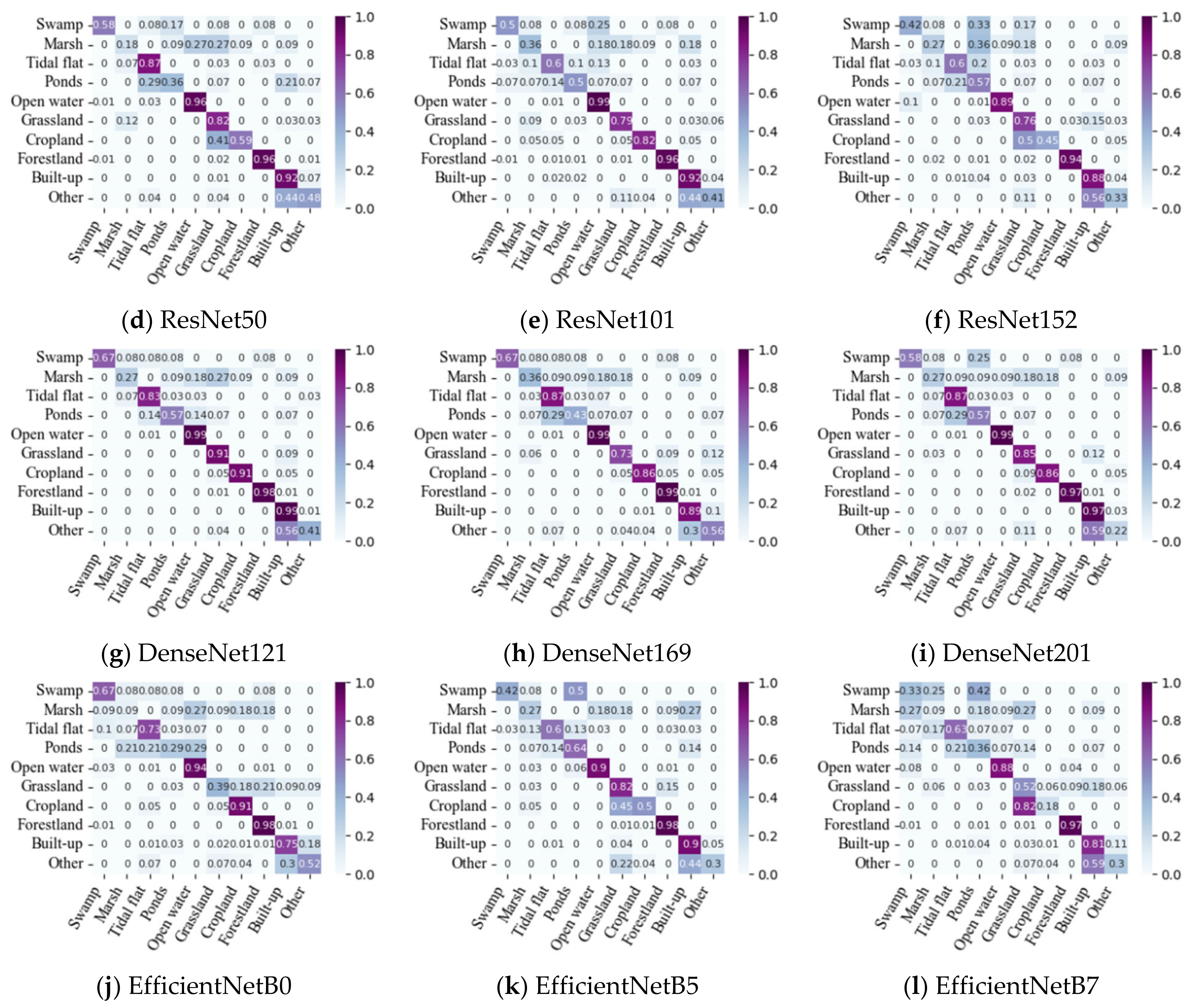
3.1. Classification Performances of Models

As shown in

Table 3. The overall performance evaluation of each model.

Model	Metric			Metric
	OA	Kappa		OA	Kappa
VGG16	0.819	0.778	DenseNet121	0.887	0.863
ResNet50	0.831	0.796	DenseNet169	0.856	0.827
ResNet101	0.828	0.793	DenseNet201	0.861	0.832
ResNet152	0.769	0.723	EfficientNetB0	0.762	0.716
MobileNet	0.840	0.807	EfficientNetB5	0.793	0.750
MobileNetV2	0.807	0.763	EfficientNetB7	0.706	0.647

, the overall performance of each model is good. The OA values of all models were greater than 0.7, and the kappa coefficients were greater than 0.6. Compared with the performances of the same models with different layers, the overall performance differences between different types of models were greater. In general, the DenseNet models showed better effects in identifying urban wetland scenes. In particular, DenseNet121 performed best, with OA and kappa values of approximately 0.89 and 0.86, respectively.

As seen from the performance of each model in identifying the subcategories, there are great differences among models. The F1-scores obtained for different subcategories with each model are shown in Figure 4. The classification results for the forestland, open water, and built-up scenes were good, while the classification results for the marsh, other, and pond scenes were relatively poor. In general, the identifiability for wetland scenes reflected by each model was lower than that for non-wetland scenes.

It is worth noting that the subcategories misclassified by each model were mainly wetland scenes; less mixing occurred with other non-wetland scenes (Figure 5). For example, in DensNet121, the ratios of the swamp, marsh, tidal flat, pond, and open water scenes that were misclassified as non-wetland scenes were 0.08, 0.45, 0, 0.14, and 0, respectively, while all other non-wetland scenes were not misclassified as wetland scenes. This result illustrated that it is more difficult to classify wetland subcategories than non-wetland subcategories. Specifically, the accuracy of DensNet121 when identifying open water and tidal flat scenes is high, reaching 0.83 and 0.99, respectively. The ratios of correctly identified swamp and pond scenes were 0.67 and 0.57, respectively. Swamp scenes were occasionally misidentified as marsh, tidal flat, pond, or forestland scenes, and pond scenes were occasionally misidentified as tidal flat, open water, grassland, or built-up scenes. Only 0.27 of the total number of samples were correctly identified as marsh scenes, which were often misidentified as grassland or open water and occasionally as pond, cropland, or built-up scenes.

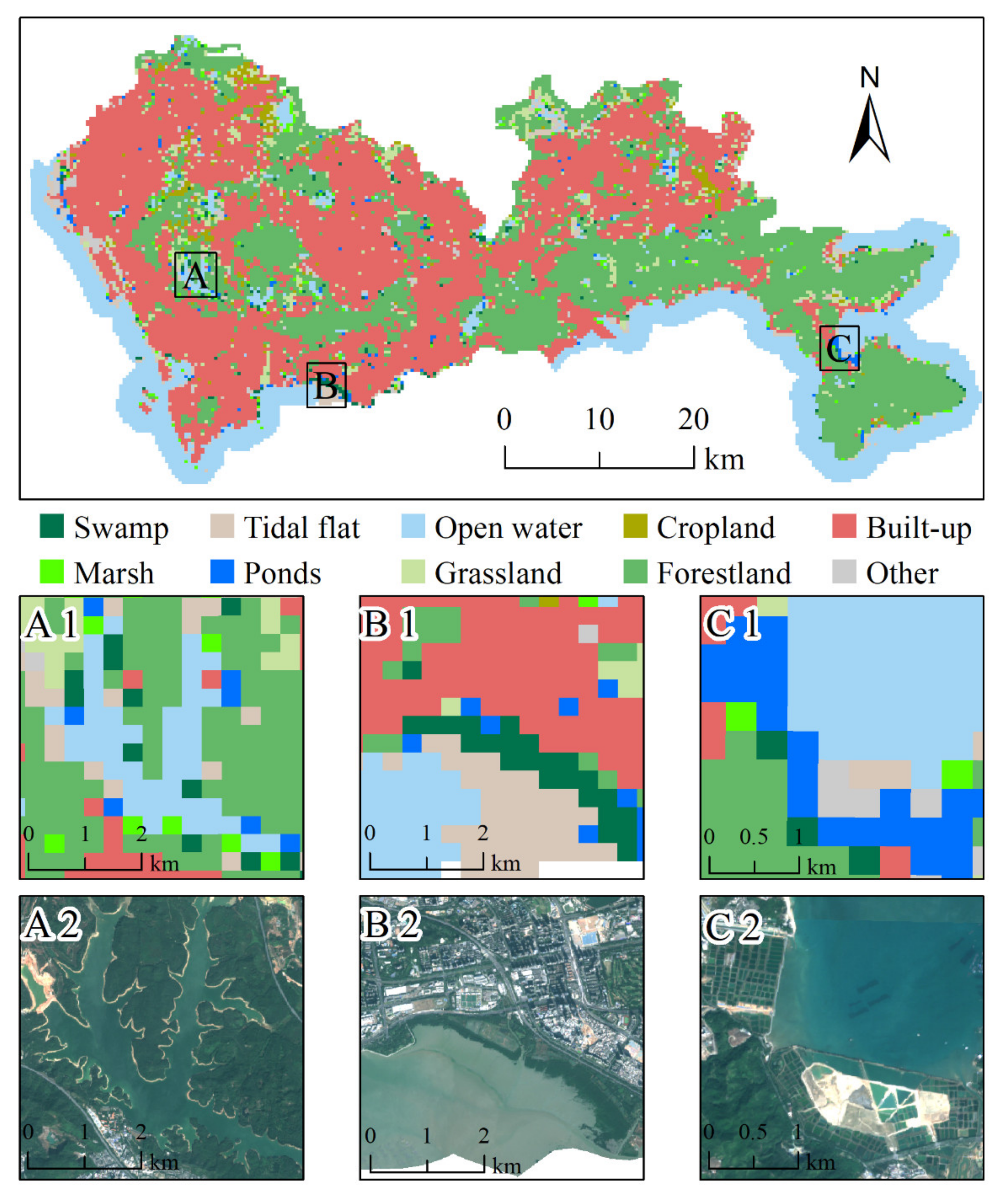
3.2. Scene Classification Results in Shenzhen

After comparing the performances of various models, we chose the DenseNet121 model to generate an urban wetland scene map of Shenzhen. As shown in Figure 6, the scene classification performance of this model was generally good. The built-up, forestland, and open water scenes constituted the main spatial pattern. To examine the classification results in more detail, we selected three important wetland areas, namely, Tiegang Reservoir, Futian Mangrove Nature Reserve, and East Coast Aquaculture Base; these areas were marked A, B, and C on the map, respectively. The classification results of these three areas showed good quality. Compared with the real remote sensing image shown in the last row of Figure 6, the classification results of these three areas can correspond to actual features. In addition, the spatial distribution of various scenes conforms to familiar ecological law. In area A, the reservoir was centered on, and surrounded by, wetland scenes, including swamps, marshes, tidal flats, and ponds. Area B shows a typical mangrove wetland pattern, ranging from open water to tidal flats and swamps. Moreover, area C reflected the dike-pond system wetland scene with Guangdong characteristics [54].

3.3. Comparison with Pixel Classification Products

As shown in

Table 4. Comparison between the scene classification results and pixel classification products.

Dataset	Number of Scenes		Evaluation Metric
	Related	Overlapping	OA	Kappa
Global30	4139	4028	0.959	0.870
GLC30	3954	3900	0.956	0.859

, in 4139 relevant scenes, the wetland area indicated by GlobeLand30 accounted for more than 50%; among these scenes, 4028 were coincident with the classification results obtained in this study, and the OA and kappa values between them reached 0.96 and 0.87, respectively. Moreover, in 3954 relevant scenes, the wetland area of GLC_FCS30 accounted for more than 50%, among which 3900 were coincident with the classification results of this study; the OA and kappa values derived between them were 0.96 and 0.86, respectively. The two products based on pixel-level classification showed good consistency with our scene classification results, indicating that the framework and methods we constructed are effective for urban wetland identification.

3.4. Spatial Pattern of Wetland Scenes in Shenzhen

As shown in Figure 7, five types of urban wetland scenes were extracted from all classification results, and standard deviation ellipses were drawn to detect their spatial patterns. First, judging from the locations, ranges, and shapes of the ellipses, the scenes were roughly distributed in an east–west pattern. This was consistent with the basic shape of Shenzhen, thus illustrating that the distribution of various wetland scenes within the city was roughly balanced. Next, we mapped the centers of the ellipses to detect the spatial pattern of the urban wetland scenes in more detail. The black cross symbol in Figure 7 is the geometric center of Shenzhen and can be used as a reference to judge the locations of other urban wetland scene centers. Obviously, the open water scenes, including a large area of coastal wetlands, were more distributed to the southeast. In addition, the remaining swamp, tidal flat, marsh, and pond scenes showed small but intensified westward distributions.

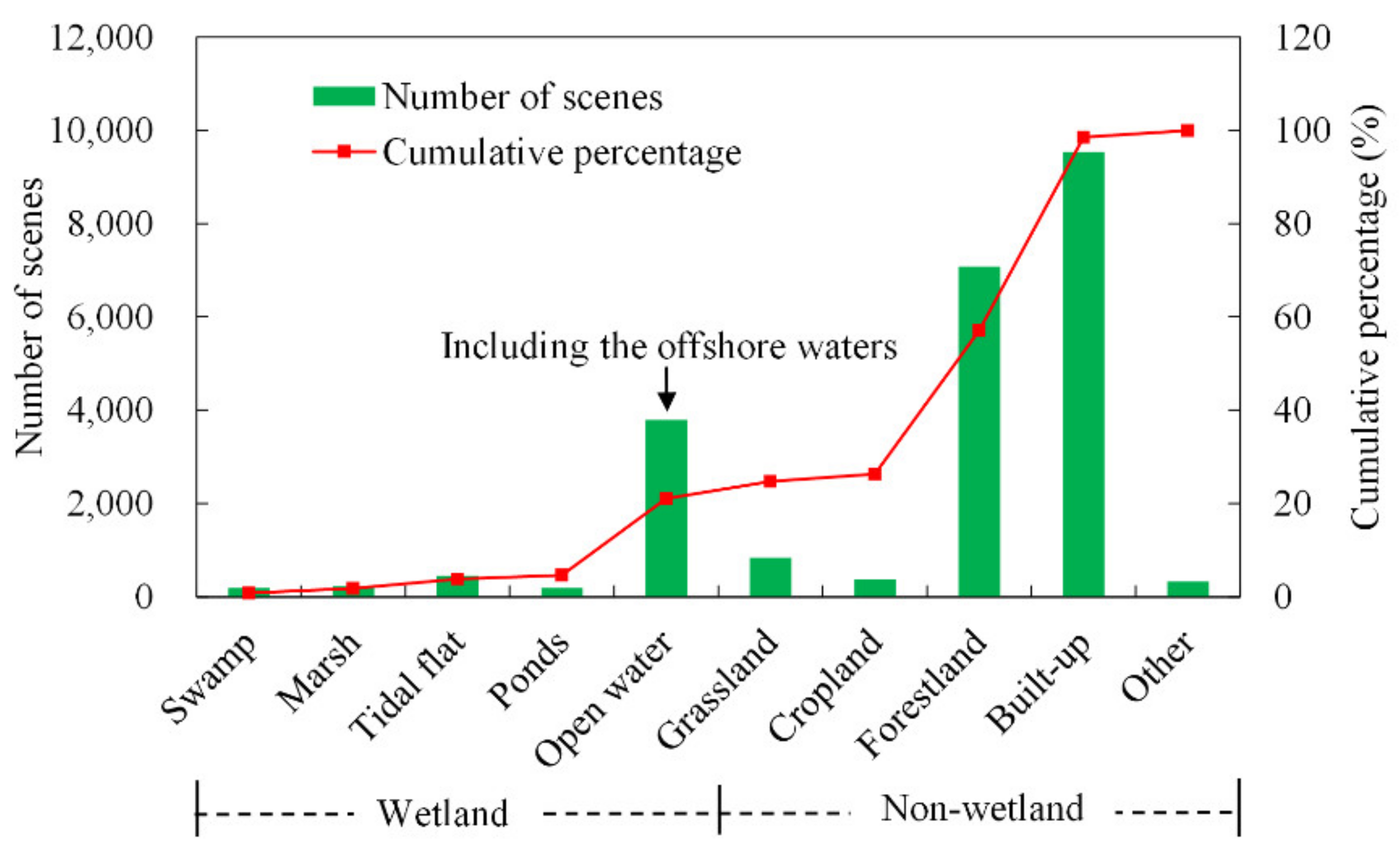
3.5. Composition of Wetland Scenes in Shenzhen

In Figure 8, the classification results of all 23,027 scenes in Shenzhen were counted. Among them, 4096 scenes were identified as urban wetland scenes, accounting for approximately 21.1% of all scenes. This percentage may seem high, but it includes the offshore waters covered by the study area and identified as open water scenes, accounting for 78% of the wetland scenes. In addition, 457, 230, 191, and 191 tidal flat, marsh, swamp, and pond scenes were identified, accounting for 9.41%, 4.73%, 3.93%, and 3.93% of the wetland scenes, respectively. The state of urban wetlands in Shenzhen is not good, and the remaining four urban wetland scenes other than open water accounted for only 4.64% of the total.

4. Discussion

An urban wetland scene may contain a mixture of multiple water bodies, tidal flats, vegetation, and even facilities. The scattered and irregular dynamic characteristics further increase their complexity in real environments. However, the traditional pixel-level classification method does not perform satisfactorily when identifying urban wetlands and is usually applied to some typical wetland cities or typical urban wetlands [12,13,14]. Therefore, this study proposed an urban wetland identification framework based on the remote sensing scene-level classification method. In a remote sensing image patch with a size of 320 m × 320 m, if the wetland covered more than 50% of the patch, the patch was defined as a wetland scene. Compared with pixel-level classification, this scene-level classification method combines multiple types of wetland semantics to identify them and includes dynamic changes that may not be observed in the scene.

This study utilized and compared 12 typical CNN models, including VGG16, ResNet50, ResNet101, ResNet152, MobileNet, MobileNetV2, DensNet121, DenseNet169, DenseNet201, EfficientNetB0, EfficientNetB5, and EfficientNetB7. Compared with classification studies conducted in natural wetlands (OAs are generally higher than 90%) [33,34], the OAs achieved in this study are lower because the classification task for urban wetlands is more complex. However, the performance of classical models in different classification tasks is similar, and the differences between different models are large. In general, the model performances gradually deteriorated from DenseNet to MobileNet to ResNet to VGG to EfficientNet. There is no substantial difference in the performance of the same model with different numbers of layers, probably because the size of the images limits its ability to learn features. Finally, the DenseNet121 model was verified as the best choice for wetland scene classification in Shenzhen. The classification results showed good consistency with the GlobeLand30 and GLC_FCS30 products classified at the pixel level, and both OAs were above 0.96. It is worth noting that our classification results identified five specific subcategories of wetlands, and the main content identified by the above two products was water bodies.

Similar to urban wetlands in other regions [13,18], the urban wetlands in Shenzhen presented an obvious scattered distribution pattern overall. Standard deviation ellipses were drawn to detect the detailed spatial pattern of the wetland scenes. Affected by coastal wetlands in the southeast and southwest, the center of the open water scenes was obviously skewed towards the southeast. The remaining wetland scenes of the swamps, tidal flats, marshes, and ponds showed only slight westward offsets. The open waters near the coast accounted for a large proportion of the wetland scenes composition, thus providing Shenzhen with extensive ecological service benefits [37,55,56]. However, the remaining urban wetland scenes other than open waters accounted for only 4.64% of the total, confirming the severity of the situation in Shenzhen in mitigating wetland degradation [57,58]. For city managers who want to achieve sustainable development, it may be an innovative idea to consider the scene classification results to formulate appropriate plans and policies for urban wetland conservation. A square scene target is easier to understand and protect than many fuzzy pixels, and a wetland scene composed of multiple components is more realistic and warrants than many static sections of land cover pixels.

With the continuous improvement in data collection capabilities, the limitations imposed by data availability on ecological research have weakened, and more attention has been given to the research frameworks and models [57]. Similarly, the high-resolution multispectral data used in this study meet the classification requirements for identifying urban wetlands, but there is still room for improvement. The Sentinel-2 images we used were resampled to a 10-meter resolution, but the input size of the CNN model was still limited. Although the very high-resolution optical images we used are clearer, they lack spectral information and are difficult to obtain and apply on the whole Shenzhen scale, so they are used only as a reference for building multispectral data samples. In the future, multispectral remote sensing images with higher resolutions and more CNN models will be considered.

5. Conclusions

Urban wetland patches in remote sensing images are usually a complex whole composed of a variety of land cover types with scattered distributions and irregular dynamic characteristics that differ from those of natural wetlands. This makes it difficult for traditional pixel-level classification methods to completely distinguish among specific wetland types, and in many cases, only water bodies can be effectively identified. Therefore, we interpret the patch types of remote sensing images at the scene level, breaking through the semantic limitation of pixel-level interpretations. In Shenzhen, we developed an urban wetland identification framework combining the latest national classification system, field surveys, very high-resolution optical images, and high-resolution multispectral images. Twelve typical CNN models were used for comparative experiments, among which the DenseNet121 model had the best performance, with OA and kappa values reaching 0.89 and 0.86, respectively. The urban wetland scenes of Shenzhen classified by the DenseNet121 model maintained good consistency with the pixel-level classification results of the GlobeLand30 and GLC_FCS30 products, and finer identification between subcategories was achieved. In addition, the standard deviation ellipse method was used to detect the spatial pattern of urban wetland scenes in Shenzhen, and we found that the spatial distribution was generally balanced in the east–west direction. In the wetland scenes, the proportion of open water was as high as 78%, and the open water center showed an obvious southward pattern. It is worth noting that the remaining urban wetland scenes, including swamps, marshes, tidal flats, and ponds, were more scattered and accounted for only 4.64% of the total area of Shenzhen, presenting a serious challenge for wetland management and protection. Therefore, we suggest that the sustainable development of Shenzhen should pay more attention to urban wetland scenes such as swamps, marshes, tidal flats, and ponds rather than being limited to land cover pixels and water body boundaries.

In summary, this study proposed an identification framework for urban wetlands based on scene-level remote sensing classification for the first time. Compared with pixel-level classification, our classification results are more conducive to being understood and accepted by city managers and can provide an effective reference for formulating appropriate urban wetland management and protection policies.

References

1. Bolund, P.; Hunhammar, S. Ecosystem services in urban areas. Ecolog. Econ. 1999, 29, 293–301. [Google Scholar] [CrossRef]
2. Ehrenfeld, J.G. Evaluating wetlands within an urban context. Ecol. Eng. 2000, 15, 253–265. [Google Scholar] [CrossRef]
3. Boyer, T.; Polasky, S. Valuing urban wetlands: A review of non-market valuation studies. Wetlands 2004, 24, 744–755. [Google Scholar] [CrossRef]
4. Gómez-Baggethun, E.; Barton, D.N. Classifying and valuing ecosystem services for urban planning. Ecolog. Econ. 2013, 86, 235–245. [Google Scholar] [CrossRef]
5. Xue, Z.S.; Hou, G.L.; Zhang, Z.S.; Lyu, X.G.; Jiang, M.; Zou, Y.C.; Shen, X.J.; Wang, J.; Liu, X.H. Quantifying the cooling-effects of urban and peri-urban wetlands using remote sensing data: Case study of cities of Northeast China. Landsc. Urban Plan. 2019, 182, 92–100. [Google Scholar] [CrossRef]
6. Patz, J.A.; Daszak, P.; Tabor, G.M.; Aguirre, A.A.; Pearl, M.; Epstein, J.; Wolfe, N.D.; Kilpatrick, A.M.; Foufopoulos, J.; Molyneux, D.; et al. Unhealthy landscapes: Policy recommendations on land use change and infectious disease emergence. Environ. Health Perspect. 2004, 112, 1092–1098. [Google Scholar] [CrossRef] [Green Version]
7. Carew, M.E.; Pettigrove, V.; Cox, R.L.; Hoffmann, A.A. The response of Chironomidae to sediment pollution and other environmental characteristics in urban wetlands. Freshw. Biol. 2007, 52, 2444–2462. [Google Scholar] [CrossRef]
8. Straka, T.M.; Lentini, P.E.; Lumsden, L.F.; Wintle, B.A.; van der Ree, R. Urban bat communities are affected by wetland size, quality, and pollution levels. Ecol. Evol. 2016, 6, 4761–4774. [Google Scholar] [CrossRef] [Green Version]
9. Townsend, K.R.; Lu, H.C.; Sharley, D.J.; Pettigrove, V. Associations between microplastic pollution and land use in urban wetland sediments. Environ. Sci. Pollut. Res. 2019, 26, 22551–22561. [Google Scholar] [CrossRef]
10. Ozesmi, S.L.; Bauer, M.E. Satellite remote sensing of wetlands. Wetl. Ecol. Manag. 2002, 10, 381–402. [Google Scholar] [CrossRef]
11. Shaikh, M.; Green, D.; Cross, H. A remote sensing approach to determine environmental flows for wetlands of the Lower Darling River, New South Wales, Australia. Int. J. Remote Sens. 2001, 22, 1737–1751. [Google Scholar] [CrossRef]
12. Guan, Y.A.; Bai, J.H.; Tian, X.; Zhi, L.H.; Yu, Z.B. Integrating ecological and socio-economic systems by carbon metabolism in a typical wetland city of China. J. Clean. Prod. 2021, 279, 123342. [Google Scholar] [CrossRef]
13. Rashid, I.; Aneaus, S. Landscape transformation of an urban wetland in Kashmir Himalaya, India using high-resolution remote sensing data, geospatial modeling, and ground observations over the last 5 decades (1965–2018). Environ. Monit. Assess. 2020, 192, 635. [Google Scholar] [CrossRef] [PubMed]
14. Zhou, H.P.; Jiang, H.; Zhou, G.M.; Song, X.D.; Yu, S.Q.; Chang, J.; Liu, S.R.; Jiang, Z.S.; Jiang, B. Monitoring the change of urban wetland using high spatial resolution remote sensing data. Int. J. Remote Sens. 2010, 31, 1717–1731. [Google Scholar] [CrossRef]
15. Zeng, Z.; Liu, Y. Fractal analysis of urban wetland shape changes using remote sensing—A case study of Nanhu Lake in Wuhan. In Proceedings of the 2008 International Workshop on Education Technology and Training & 2008 International Workshop on Geoscience and Remote Sensing, Shanghai, China, 21–22 December 2008; pp. 298–301. [Google Scholar]
16. Xu, X.; Ji, W. Knowledge-based algorithm for satellite image classification of urban wetlands. In Proceedings of the International Conference of Computational Methods in Sciences and Engineering, Athens, Greece, 4–7 April 2014; pp. 285–288. [Google Scholar]
17. Bareuther, M.; Klinge, M.; Buerkert, A. Spatio-temporal dynamics of algae and macrophyte cover in urban lakes: A remote sensing analysis of Bellandur and Varthur Wetlands in Bengaluru, India. Remote Sens. 2020, 12, 3843. [Google Scholar] [CrossRef]
18. Ji, W.; Xu, X.F.; Murambadoro, D. Understanding urban wetland dynamics: Cross-scale detection and analysis of remote sensing. Int. J. Remote Sens. 2015, 36, 1763–1788. [Google Scholar] [CrossRef]
19. He, C.Y.; Tian, J.; Shi, P.J.; Hu, D. Simulation of the spatial stress due to urban expansion on the wetlands in Beijing, China using a GIS-based assessment model. Landsc. Urban Plan. 2011, 101, 269–277. [Google Scholar] [CrossRef]
20. Cheng, G.; Li, Z.P.; Yao, X.W.; Guo, L.; Wei, Z.L. Remote sensing image scene classification using bag of convolutional features. IEEE Geosci. Remote Sens. Lett. 2017, 14, 1735–1739. [Google Scholar] [CrossRef]
21. Cheng, G.; Han, J.W.; Lu, X.Q. Remote Sensing Image Scene Classification: Benchmark and State of the Art; IEEE: New York, NY, USA, 2017; pp. 1865–1883. [Google Scholar]
22. Blaschke, T.; Strobl, J. What’s wrong with pixels? Some recent developments interfacing remote sensing and GIS. Z. Geoinf. 2001, 6, 12–17. [Google Scholar]
23. Amiri, K.; Farah, M.; Leloglu, U.M. BoVSG: Bag of visual SubGraphs for remote sensing scene classification. Int. J. Remote Sens. 2020, 41, 1986–2003. [Google Scholar] [CrossRef]
24. Zhang, J.M.; Lu, C.Q.; Li, X.D.; Kim, H.J.; Wang, J. A full convolutional network based on DenseNet for remote sensing scene classification. Math. Biosci. Eng. 2019, 16, 3345–3367. [Google Scholar] [CrossRef] [PubMed]
25. Cheng, G.; Xie, X.X.; Han, J.W.; Guo, L.; Xia, G.S. Remote sensing image scene classification meets deep learning: Challenges, methods, benchmarks, and opportunities. IEEE J. Sel. Top. Appl. Earth Observ. Remote Sens. 2020, 13, 3735–3756. [Google Scholar] [CrossRef]
26. Simonyan, K.; Zisserman, A. Very deep convolutional networks for large-scale image recognition. arXiv 2014, arXiv:1409.1556. [Google Scholar]
27. He, K.M.; Zhang, X.Y.; Ren, S.Q.; Sun, J. Identity mappings in meep residual networks. arXiv 2014, arXiv:1603.05027v3. [Google Scholar]
28. Huang, G.; Liu, Z.; van der Maaten, L.; Weinberger, K.Q. Densely connected convolutional networks. In Proceedings of the 2017 IEEE Conference on Computer Vision and Pattern Recognition, Honolulu, HI, USA, 21–26 July 2017; pp. 2261–2269. [Google Scholar]
29. Howard, A.G.; Zhu, M.; Chen, B.; Kalenichenko, D.; Wang, W.; Weyand, T.; Andreetto, M.; Adam, H. Mobilenets: Efficient convolutional neural networks for mobile vision applications. arXiv 2017, arXiv:1704.04861. [Google Scholar]
30. Sandler, M.; Howard, A.; Zhu, M.L.; Zhmoginov, A.; Chen, L.C. MobileNetV2: Inverted residuals and linear bottlenecks. In Proceedings of the 2018 IEEE/CVF Conference on Computer Vision and Pattern Recognition, Salt Lake City, UT, USA, 18–23 June 2018; pp. 4510–4520. [Google Scholar]
31. Tan, M.X.; Le, Q.V. EfficientNet: Rethinking model scaling for convolutional neural networks. arXiv 2019, arXiv:1905.11946. [Google Scholar]
32. Wang, H.; Wen, X.; Wang, Y.; Cai, L.; Liu, Y. China’s land cover fraction change during 2001–2015 based on remote sensed data fusion between MCD12 and CCI-LC. Remote Sens. 2021, 13, 341. [Google Scholar] [CrossRef]
33. Rezaee, M.; Mahdianpari, M.; Zhang, Y.; Salehi, B. Deep convolutional neural network for complex wetland classification using optical remote sensing imagery. IEEE J. Sel. Top. Appl. Earth Observ. Remote Sens. 2018, 11, 3030–3039. [Google Scholar] [CrossRef]
34. Mahdianpari, M.; Salehi, B.; Rezaee, M.; Mohammadimanesh, F.; Zhang, Y. Very deep convolutional neural networks for complex land cover mapping using multispectral remote sensing imagery. Remote Sens. 2018, 10, 1119. [Google Scholar] [CrossRef] [Green Version]
35. Gunen, M.A. Performance comparison of deep learning and machine learning methods in determining wetland water areas using EuroSAT dataset. Environ. Sci. Pollut. Res. 2021, in press. [Google Scholar] [CrossRef]
36. Shi, P.J.; Yuan, Y.; Zheng, J.; Wang, J.A.; Ge, Y.; Qiu, G.Y. The effect of land use/cover change on surface runoff in Shenzhen region, China. Catena 2007, 69, 31–35. [Google Scholar] [CrossRef]
37. Li, T.H.; Li, W.K.; Qian, Z.H. Variations in ecosystem service value in response to land use changes in Shenzhen. Ecol. Econ. 2010, 69, 1427–1435. [Google Scholar]
38. Meng, L.T.; Sun, Y.; Zhao, S.Q. Comparing the spatial and temporal dynamics of urban expansion in Guangzhou and Shenzhen from 1975 to 2015: A case study of pioneer cities in China’s rapid urbanization. Land Use Pol. 2020, 97, 104753. [Google Scholar] [CrossRef]
39. Liengpunsakul, S. Artificial intelligence and sustainable development in China. Chin. Econ. 2021, 54, 235–248. [Google Scholar] [CrossRef]
40. Yu, B.B. Ecological effects of new-type urbanization in China. Renew. Sust. Energ. Rev. 2021, 135, 110239. [Google Scholar] [CrossRef]
41. Li, H.; Chen, P.J.; Grant, R. Built environment, special economic zone, and housing prices in Shenzhen, China. Appl. Geogr. 2021, 129, 102429. [Google Scholar] [CrossRef]
42. Zhao, R.; Wu, K.N.; Li, X.L.; Gao, N.; Yu, M.M. Discussion on the unified survey and evaluation of cultivated land quality at county scale for China’s 3rd National Land Survey: A case study of Wen County, Henan Province. Sustainability 2021, 13, 2513. [Google Scholar] [CrossRef]
43. Ji, F.J.; Meng, J.H.; Cheng, Z.Q.; Fang, H.T.; Wang, Y.N. Crop yield estimation at field scales by assimilating time series of Sentinel-2 data into a modified CASA-WOFOST coupled model. IEEE Trans. Geosci. Remote Sens. 2022, 60, 4400914. [Google Scholar] [CrossRef]
44. Slagter, B.; Tsendbazar, N.E.; Vollrath, A.; Reiche, J. Mapping wetland characteristics using temporally dense Sentinel-1 and Sentinel-2 data: A case study in the St. Lucia wetlands, South Africa. Int. J. Appl. Earth Obs. Geoinf. 2020, 86, 102009. [Google Scholar] [CrossRef]
45. Eid, A.N.M.; Olatubara, C.O.; Ewemoje, T.A.; El-Hennawy, M.T.; Farouk, H. Inland wetland time-series digital change detection based on SAVI and NDWI indecies: Wadi El-Rayan lakes, Egypt. Remote Sens. Appl. Soc. Environ. 2020, 19, 100347. [Google Scholar] [CrossRef]
46. Schmitt, M.; Hughes, L.; Qiu, C.; Zhu, X.X. Aggregating cloud-free Sentinel-2 images with Google Earth Engine. In Proceedings of the PIA19: Photogrammetric Image Analysis, Munich, Germany, 16 September 2019; pp. 145–152. [Google Scholar]
47. Chen, J.; Ban, Y.; Li, S. Open access to Earth land-cover map. Nature 2014, 514, 434. [Google Scholar]
48. Zhang, X.; Liu, L.; Chen, X.; Gao, Y.; Xie, S.; Mi, J. GLC_FCS30: Global land-cover product with fine classification system at 30 m using time-series Landsat imagery. Earth Syst. Sci. Data 2021, 13, 2753–2776. [Google Scholar] [CrossRef]
49. Deng, J.; Dong, W.; Socher, R.; Li, L.J.; Li, K.; Li, F.F. ImageNet: A large-scale hierarchical image database. In Proceedings of the 2009 IEEE Conference on Computer Vision and Pattern Recognition, Miami, FL, USA, 20–25 June 2009; pp. 248–255. [Google Scholar]
50. Wen, Y.D.; Zhang, K.P.; Li, Z.F.; Qiao, Y. A discriminative feature learning approach for deep face recognition. In Proceedings of the Computer Vision—ECCV 2016, Amsterdam, The Netherlands, 11–14 October 2016; pp. 499–515. [Google Scholar]
51. Goutte, C.; Gaussier, E. A probabilistic interpretation of precision, recall and F-score, with implication for evaluation. In Proceedings of the ECIR 2005: Advances in Information Retrieval, Santiago de Compostela, Spain, 21–23 March 2005; pp. 345–359. [Google Scholar]
52. Pashaei, M.; Kamangir, H.; Starek, M.J.; Tissot, P. Review and evaluation of deep learning architectures for efficient land cover mapping with UAS hyper-spatial imagery: A case study over a wetland. Remote Sens. 2020, 12, 959. [Google Scholar] [CrossRef] [Green Version]
53. Peng, J.; Chen, S.; Lu, H.L.; Liu, Y.X.; Wu, J.S. Spatiotemporal patterns of remotely sensed PM2.5 concentration in China from 1999 to 2011. Remote Sens. Environ. 2016, 174, 109–121. [Google Scholar] [CrossRef]
54. Korn, M. The dike pond concept: Sustainable agriculture and nutrient recycling in China. Ambio 1996, 25, 6–13. [Google Scholar]
55. Huang, X.; Han, X.P.; Ma, S.; Lin, T.J.; Gong, J.Y. Monitoring ecosystem service change in the City of Shenzhen by the use of high-resolution remotely sensed imagery and deep learning. Land Degrad. Dev. 2019, 30, 1490–1501. [Google Scholar] [CrossRef]
56. Yang, R.; Ren, F.; Xu, W.; Ma, X.; Zhang, H.; He, W. China’s ecosystem service value in 1992–2018: Pattern and anthropogenic driving factors detection using Bayesian spatiotemporal hierarchy model. J. Environ. Manag. 2022, 302, 114089. [Google Scholar] [CrossRef]
57. Peng, J.; Liu, Y.X.; Wu, J.S.; Lv, H.L.; Hu, X.X. Linking ecosystem services and landscape patterns to assess urban ecosystem health: A case study in Shenzhen City, China. Landsc. Urban Plan. 2015, 143, 56–68. [Google Scholar] [CrossRef]
58. Zhou, H.J.; Shi, P.J.; Wang, J.A.; Yu, D.Y.; Gao, L. Rapid urbanization and implications for river ecological services restoration: Case study in Shenzhen, China. J. Urban Plan. Dev 2011, 137, 121–132. [Google Scholar] [CrossRef]
Figure 1. Overall urban wetland identifying workflow followed in this study.
Ijgi 11 00131 g001
Figure 2. Study area: (a) Is the location map of Shenzhen in Guangdong Province in China; (b) is the false color Sentinel-2 remote sensing image (bands 8, 4, and 3) of Shenzhen.
Ijgi 11 00131 g002
Figure 3. The indigenous classification system of Shenzhen.
Ijgi 11 00131 g003
Figure 4. The F1-scores of different subcategories in each model.
Ijgi 11 00131 g004
Figure 5. Tables containing the normalized confusion matrices of different models.
Ijgi 11 00131 g005aIjgi 11 00131 g005b
Figure 6. Mapping scene classification results derived from the DenseNet121 model and comparison of true color high-resolution images (bands 4, 3 and 2). (A) Tiegang Reservoir, (B) Futian Mangrove Nature Reserve, and (C) East Coast Aquaculture Base.
Ijgi 11 00131 g006
Figure 7. Spatial pattern of the urban wetland scenes of Shenzhen.
Ijgi 11 00131 g007
Figure 8. Composition of scene classification results.
Ijgi 11 00131 g008