
A Fine-Grain Batching-Based Task Allocation Algorithm for Spatial Crowdsourcing


1
The Academy of Digital China (Fujian), Fuzhou University, Fuzhou 350108, China
2
College of Computer and Data Science/College of Software, Fuzhou University, Fuzhou 350108, China
3
Key Lab of Spatial Data Mining & Information Sharing, MOE, Fuzhou University, Fuzhou 350108, China
*
Author to whom correspondence should be addressed.
ISPRS Int. J. Geo-Inf. 2022, 11(3), 203; https://doi.org/10.3390/ijgi11030203
Submission received: 30 December 2021
/
Revised: 10 March 2022
/
Accepted: 12 March 2022
/
Published: 17 March 2022
Abstract
:Task allocation is a critical issue of spatial crowdsourcing. Although the batching strategy performs better than the real-time matching mode, it still has the following two drawbacks: (1) Because the granularity of the batch size set obtained by batching is too coarse, it will result in poor matching accuracy. However, roughly designing the batch size for all possible delays will result in a large computational overhead. (2) Ignoring non-stationary factors will lead to a change in optimal batch size that cannot be found as soon as possible. Therefore, this paper proposes a fine-grained, batching-based task allocation algorithm (FGBTA), considering non-stationary setting. In the batch method, the algorithm first uses variable step size to allow for fine-grained exploration within the predicted value given by the multi-armed bandit (MAB) algorithm and uses the results of pseudo-matching to calculate the batch utility. Then, the batch size with higher utility is selected, and the exact maximum weight matching algorithm is used to obtain the allocation result within the batch. In order to cope with the non-stationary changes, we use the sliding window (SW) method to retain the latest batch utility and discard the historical information that is too far away, so as to finally achieve refined batching and adapt to temporal changes. In addition, we also take into account the benefits of requesters, workers, and the platform. Experiments on real data and synthetic data show that this method can accomplish the task assignment of spatial crowdsourcing effectively and can adapt to the non-stationary setting as soon as possible. This paper mainly focuses on the spatial crowdsourcing task of ride-hailing.
1. Introduction
Crowdsourcing is a computing paradigm whereby humans actively or passively participate in the procedure of computing, especially for tasks that are intrinsically easier for humans than for computers [1]. With the popularization of advanced mobile devices, a new crowdsourcing framework, spatial crowdsourcing (SC) [2,3,4,5,6,7,8], harnesses the potential of the crowd to perform real-world tasks with a strong spatial nature that are not supported by conventional crowdsourcing techniques [9]. On excellent spatial crowdsourcing platforms such as Uber [10], Waze [11], GrubHub [12], and Gigwalk [13], task requesters can send spatial tasks to SC servers, which employ smart device carriers as workers to physically move to designated locations to complete these spatial tasks. Crowdsourcing workers are participants in the process of spatial crowdsourcing task allocation, also known as task executors.
How to assign large-scale tasks to the corresponding crowdsourcing task executors is the first challenge that the spatial crowdsourcing platform faces; that is, task assignment. The purpose of task assignment is to arrange tasks for suitable task performers according to multiple objectives. Task allocation in spatial crowdsourcing is generally defined as: Given a group of tasks and a group of task performers, task allocation is the process of arranging tasks and task performers for specific goals under the premise of meeting spatial constraints, time constraints, or other constraints. The real-time matching method [14,15,16] can give the allocation result as soon as possible.
In fact, a real application might not strictly require tasks to be assigned immediately. By waiting for a reasonably short period of time, it is feasible for the system to implement local static allocation in batch mode. However, how to theoretically select the optimal single batch or adjust the batch size in real time to significantly improve the effectiveness of the task allocation algorithm is still an open problem. Most of the existing spatial crowdsourcing batch modes mostly adopt fixed batch size and test the influence of different batch sizes on the task allocation algorithm in the experimental stage.
Kazemi et al. [17,18] adopted the batch strategy and simplified the bipartite graph as an instance of the maximum flow problem, obtaining accurate results using the basic strategy based on the Ford–Fulkerson algorithm. However, the fixed batch mode does not perform well in practical application, with a constantly changing demand density, therefore the real-time batch adjustment strategy has attracted more and more attention from researchers [19,20,21,22,23]. Qian et al. [24] proposed an adaptive batch processing mechanism based on spatial crowdsourcing to take better care of user experience and more realistic situations. Due to the advantages of the design mechanism, some traditional task allocation methods can also be combined with the adaptive batch processing mechanism, which improves the efficiency of online dynamic task allocation and shows good compatibility. According to this framework, they designed a dynamic batch adjustment scheme based on the multi-armed bandit (MAB) algorithm, which is an algorithm used to infer the next most suitable batch size through historical data. At the same time, they also took the average waiting time of users as the optimization goal, so as to enhance the user experience and better meet the needs of the real situation.
However, this algorithm does not fully consider the non-stationarity of the optimal batch size. In our research, we optimize the task allocation effect of spatial crowdsourcing by tracking the dynamic change of the optimal batch size. In addition, if there are too many kinds of optional batches in the MAB algorithm, the algorithm overhead will be greatly increased. There are too few optional batch types, which will affect the accuracy of batching and lead to poor task allocation effects. We take a fine-grained batching approach and consider the benefits of multiple stakeholders simultaneously. Overall, the main contributions of this article are as follows:
- We propose a fine-grained batching-based task allocation algorithm (FGBTA) for the online allocation problem in batch mode (OAPB) to achieve precise batching and improve allocation efficiency;
- We introduce the non-stationary setting to consider the dynamic changes of the environment and use two concept drifts (a phenomenon that a target variable changes over time) to verify the effectiveness of the algorithm in experiments;
- We verify the effectiveness and efficiency of the algorithm on synthetic data and real data. Experimental results show that our method is superior to the compared methods in terms of overall utility and waiting time.
In the remainder of the paper, we review relevant studies in Section 2 and formally define the OAPB problem in Section 3. Section 4 formally introduces the FGBTA method. The Section 5 sets up experiments to evaluate our solutions. The Section 6 summarizes this paper and looks forward to further research.
2. Related Work
Under the framework of spatial crowdsourcing, the online allocation problem based on batch mode is studied, and an adaptive batch processing method based on MAB is adopted. Therefore, in the related research section, we review the following three topics.
2.1. Crowdsourcing and Geographic Information Crowdsourcing
Crowdsourcing [25,26,27,28,29] refers to the process of collecting information or inputting tasks from a large number of crowds, usually through the Internet [30]. Crowdsourcing is an online distributed problem-solving paradigm, in which an individual, company, or organization publishes defined task(s) to the dynamic crowd through a flexible open call to leverage human intelligence, knowledge, skill, work, and experience [31]. Currently, it widely supports various applications and has made remarkable achievements.
Many researchers have studied crowdsourcing about geographic information [32,33,34,35]. Goodchild et al. [36] studied the potential role of volunteered geographic information (VGI) [37,38] in disaster management, which is closely related to the concept of crowdsourcing. They not only reviewed the field of the VGI, but also studied the correlation between crowdsourcing data quality and disaster management, and discussed four forest fires that affected the Santa Barbara area as an example. Basiri and Hacklay et al. [39] focused on the challenges and future directions of crowdsourcing geospatial data, especially on the problems caused by data quality and VGI deviation. They believed that VGI can not only be used as a method of making maps, but also as a complex, more democratic, reproducible, open, and reliable system, which can involve the society and promote diversity, cooperation, and wider participation. Hacklay et al. [40] regarded geographic citizen science as a field wherein crowdsourcing geographic information and citizen science are combined, and crowdsourcing allows ordinary people to participate in scientific work, because the data they generate has obvious geographical characteristics. Khajwal et al. [41] improved the effectiveness of crowdsourcing in post-disaster damage assessment by enhancing the content and reliability of information gathered through public participation. The research presented a novel framework for the quantification and reduction of uncertainty in the outcome of participatory damage assessment. Vrbik [42] introduced a process of collecting non-standardized place names in two cities of the Czech Republic. The collection process is carried out by crowdsourcing using a network map application specially created for this purpose.
Numerous spatial crowdsourcing applications have appeared in developed areas such as North America and Europe. Since 2009, the successful Geo-Wiki Project [43] has been running. The Geo-Wiki project is an online volunteer network created to eliminate location incompatibilities and increase the accuracy of global land cover maps. The Global Earthquake Model (GEM) [44] project uses the concept of crowdsourcing. It is an international forum where organizations and individuals gather to develop, use, and share tools and resources to make an unbiased assessment of earthquake risk. The experimental project Clickworkers [45] was launched by NASA in 2000. This project aimed at identifying and classifying craters on Mars, and thousands of participants analyzed every image in the database. In the above projects, data is actively generated and submitted, which means that a specific mobile application or service is established to collect reports generated by users. This crowdsourcing is called active crowdsourcing. Even without voluntary contributors, crowdsourcing may be activated. This crowdsourcing is called passive crowdsourcing. For example, people now consume and generate geographic information as new geographic information sources at any time through Flickr, Twitter, Facebook, and Instagram.
2.2. Online Allocation in Batch Mode
Kazemi et al. [17] firstly applied the batch method to solve the task allocation problem of spatial crowdsourcing, and proposed three solutions to the maximum cardinality problem in batch mode: Greedy Strategy (GR), Lease Location Entropy Priority (LLEP), and Nearest Neighbor Priority Strategy (NNP). Although they clearly and completely described the specific matching methods, spatial tasks, and crowdsourcing workers’ participation in the matching within fixed time intervals, they did not consider the influence of the interval length (batch size) on the matching performance.
In the scheduling framework based on batch processing, Wang et al. [46] adopted the reinforcement learning method of Q-learning to adaptively change the batch size and gave the theoretical analysis results ensuring the competition ratio. Different from Wang et al., who focused on the overall utility of the platform, Qian et al. [24] focused on the effects of user experience and supply and demand on batching. They introduced the MAB problem into the batching mechanism and improved the ϵ-greedy method. In our work, we comprehensively consider the requirements of requests, crowdsourcing workers, and platforms, and balance and improve the benefits of all these aspects by constructing reasonable optimization objectives. Sun et al. [47] firstly predicted the number of future spatial tasks and crowdsourcing workers through the GRU deep learning model, and then studied the adaptive batching strategy based on DQN and DDQN to solve the task allocation problem. For specific spatial crowdsourcing applications and ride-hailing applications, Qin et al. [21] customized a series of methods based on reinforcement learning to overcome the dimension curse and sparse reward problems. Meanwhile, this work also provided a solution for the balance of spatial partition between the state representation error of asynchronous matching and the optimal gap. Aiming at the bottleneck matching problem, Wang [48] proposed an adaptive holding strategy based on reinforcement learning, and gave the theoretical results of the stochastic algorithm of performance boundary. Due to the dynamic characteristics of spatial tasks and crowdsourcing workers’ arrival, the non-stationarity of optimal batch size has not been fully considered in the above research. By tracking the dynamic changes of the optimal batch size, the task allocation effect of spatial crowdsourcing can be optimized.
2.3. Multi-Armed Bandit (MAB)
The problem of MAB is a classic problem in probability theory, which belongs to the category of reinforcement learning. The problem is as follows: a gambler enters a casino and faces a gambling machine with arms. He does not know the real profit of each arm in advance. Every time he plays, he can pull down one arm and receive profit. He needs to select an arm drop each time to obtain the maximum payoff (or minimum regret) for round .
With stationary setting [49,50,51], the reward distribution of each arm in all rounds is fixed. A simple and effective way to deal with the problem is -greedy. It selects the optimal arm (called “exploitation”) with a probability of 1- and randomly selects the arm (called “exploration”) with a probability of . The limitation of this method is that the probability of selection of all arms is equal during exploration, and the observed reward information is not fully utilized. Upper Confidence Bound (UCB) [52,53,54,55,56] is an optimistic strategy for dealing with uncertain environments. The Upper Bound of Confidence is calculated by counting the selected times of each arm, and this algorithm can obtain the regret value of . The limitation of this method is that it is necessary to calculate and update the upper bound of confidence interval of each arm. When the number of arms is too large, the computational cost is too high. Thompson sampling [57,58,59,60,61] was first put forward by Thompson in 1933, also known as posterior sampling and probability matching. Its basic idea is this: firstly, assume that the reward distribution parameter of each arm is a simple prior distribution, and then select the optimal arm according to the updated posterior probability. Thompson sampling algorithm works well, but its performance is poor in time sensitivity problems. Although there has been abundant and effective research on MAB algorithms in stationary environments, many methods are still being explored for more realistic non-stationary environments.
In non-stationary circumstances, the reward distribution of each arm in round may change over time. Cao et al. [62] perceived changes in the environment by detecting changes in the average value of arm reward experience. They developed M-UCB algorithm, which combined the UCB method with a change point detection component based on sliding window (SW) and solved the problem of MAB with piecewise stability. This method adopts a change detection algorithm to monitor environment changes and perform restart, which is an active adaptive strategy. Another strategy is known as passive adaptive strategy. Trovo et al. [63] used the Thompson Sampling (SW-TS) method in SW to deal with two different forms of non-stationary environment: sudden change and smooth change in a unified way. This method uses the reward distribution of the information updating arm in the last n rounds. Cavenaghi et al. [64] proposed three versions of F-DSW TS algorithm: pessimistic version, optimistic version, and average version. The discount factor and the SW method were added to the reward function, which not only enhanced the influence of recent awards but also retained the influence of the historical awards, so as to achieve the purpose of adaptively tracking the optimal award allocation.
Concept drift [65,66,67,68,69] refers to the unpredictable change of the statistical characteristics of the target variables that the model tries to predict with the passage of time. The existence of a concept drift makes the prediction result inaccurate, resulting in a suboptimal decision [70]. In this study, we suggest that the distribution of arm reward changes over time. Concept drift has the following four types: (1) sudden drift, which occurs suddenly in a short period of time, and the new concept replaces the old one; (2) gradual drift, in which the new concept gradually replaces the old concept in a period of time; (3) incremental drift: the old concept gradually develops to the new concept in a period of time; (4) reoccurring drift: old concept will reappear after a period of time.
3. Problem Statement
In this section, we give the basic definition of spatial crowdsourcing task allocation, and then we formally define the optimization objective of task allocation.
3.1. SC Allocation-Related Definitions
Definition 1
(Requester). The requester firstly designs the task and sets the constraints that need to be met when executing the task, and then publishes it on the spatial crowdsourcing platform, waiting for crowdsourcing workers to accept the task.
Definition 2
(Worker). A crowdsourcing worker is a participant in the process of spatial crowdsourcing task allocation. After accepting the task, he needs to move to a specific geographical location as soon as possible to perform the spatial task. A worker is represented by .
- represents the time stamp when he appears ongeographic coordinates. Considering that, in practical applications, workers (such as taxi drivers) tend to move dynamically and that their geographical coordinates are constantly changing, we assume that, if a worker is not assigned a suitable task within a certain period, the worker needs to update his geographical locationand the corresponding appearance time, and then appear on the platform as a new worker, that is,disappears andappears.
- indicates the speed at which workers move to the task location.
- andrespectively represent the latitude and longitude of workers’ geographical position at.
- means that crowdsourcing workers are near the geographic coordinate ofin the period, and they can still use this coordinate to express their geographic position. It is worth noting that, if crowdsourcing workers cannot find a suitable task to match during, they will re-participate in the platform matching process at a new time stamp and a new location.
- represents the acceptable order radius for crowdsourcing workers. If the order distance exceeds the acceptable radius, we think that the task position is too far away, and reckless dispatch will greatly reduce the experience of both sides.
Definition 3
(Spatial Task). Different from traditional tasks, spatial tasks carry geographic information and require crowdsourcing workers to be present at the mission location. A task is defined by .
- represents the release timestamp of the task, that is, the time when the task arrives at the server.
- andrepresent the latitude and longitude of the geographical location of the task, respectively.
- indicates the duration of the task, andis the expiration time stamp of the task.
- represents the specific description of the spatial task. In the application of taxi order dispatch, its specific description is mainly composed of the customer’s destination, namely, whererepresents the latitude of the task destination andrepresents the longitude of the task destination.
Definition 4
(Matching Triplet). The matching triplet consists of crowdsourcing workers, spatial tasks, and allocation time, that is, . is the matching time of spatial task and worker .
3.2. Problem Definitions
Definition 5
(Batch Size). The batch size is represented by , which means that the platform allocates tasks once every b time units. represents the time interval between the -th and -th task assignments. Fixed batch means that the batch size is a constant value and will not change with the variation of the data input stream, namely . Variable batch means that the batch size will increase or decrease with the variation of data input stream. is a batch set, which records the size of each batch. It is expressed as .
Definition 6
(Waiting Time). In this paper, we mainly focus on the spatial crowdsourcing task of ride-hailing. Therefore, the waiting time in this scenario goes through three stages: (1) Firstly, the requester issues the spatial task ; (2) Then, in the process of task allocation, the platform finds a suitable crowdsourcing worker for the requester; (3) Finally, the crowdsourcing worker receives the requester at the timestamp . The subscript in indicates the timestamp when the requester meets with the crowdsourcing worker and finishes waiting.
The waiting timeof the requester is composed of two parts: (1) The waiting time for task assignment, that is, the difference between task assignment time and release time is expressed as. (2) The waiting pickup time consumed by crowdsourcing workers to receive requesters, namely, the ratio of spatial distance to speed, is expressed as.represents the distance between spatial task and worker. Therefore, the total waiting time of the requester is defined as
Definition 7
(Order Reward). Order Reward refers to the profit that crowdsourcing workers can obtain when completing the spatial task. In the application of ride-hailing, the rewards for workers are often related to the distance to their destination. Therefore, we use distance to express order reward, which is represented by
Definition 8
(Success Rate of Allocation). For crowdsourcing platforms, the more tasks they allocate, the more benefits they can earn. We use to represent the success rate of allocation, where and represent the spatial task set and matching pair set after all tasks are completed, respectively, and the meaning of the count function is to count the total number of sets.
Definition 9
(Matching Utility). Requesters, workers, and platforms are the three related sides of spatial crowdsourcing task allocation, and they attach different importance to the allocation factors. In the application of ride-hailing, the requester hopes that the crowdsourcing worker will pick up the driver as soon as possible and reduce the waiting time. Crowdsourcing workers are more likely to be assigned to long-distance orders, which increases the income and reduces the idle rate of cars. The platform hopes to improve the success rate of matching, meet the requirements of both supply and demand sides, and gain more profits. In this paper, the matching utility score comprehensively measures the benefits of three sides by using three factors: the waiting time of user, the reward of order, and the success rate of allocation. The matching utility between tasks and crowdsourcing workers is calculated by weight value and normalized value.
Weight value:
- the waiting time of user:
- the reward of order:
- the success rate of matching:
Normalized function:
There are two reasons for using normalization function here: Firstly, normalization can transform dimensional expression into dimensionless expression. The normalized data is in the same order of magnitude. It can eliminate the influence of dimensions and dimension units between indicators. Secondly, normalization can convert data into decimals between (0, 1), which is convenient for data processing.
- Wait time normalization function:
- Order reward normalization function:
- Success rate of matching normalization function:
In order to keep consistency with other indicators, we also calculated normalization for the success rate, where the default value ofis 1 and the default value ofis 0.
The utility score of a single matchis calculated by the following formula:
It is worth noting that the subscriptis the same asinabove. The subscriptinindicates the timestamp when the requester meets with the crowdsourcing worker and finishes waiting.
The total utility scoreis calculated by the following formula, whereis the average utility andis weight of.
Definition 10
(Online Allocation Problem in Batch Mode, OAPB). In a static scenario (also known as offline scenario), it is assumed that the platform knows all the spatiotemporal information about participants from the beginning, including the arrival time and location of tasks and workers. Different from an offline scenario, an online scenario represents most of the real scenarios of spatial crowdsourcing, in which spatial tasks and crowdsourcing workers arrive dynamically and their spatiotemporal information cannot be obtained in advance before the time is up. Due to the limited information obtained by the greedy algorithm of instant matching, we cut the time stream into set by batch processing. The objective of an online allocation problem in batch mode is to find a set of matching pair to maximize the matching utility .
4. Fine-Grained Batching-Based Task Allocation Algorithm (FGBTA)
In this section, we firstly introduce the basic idea of fine granularity batching, and then design the FGBTA algorithm combined with an in-batch matching algorithm to solve the online allocation problem in batching mode.
4.1. Basic Idea
The task assignment process in batch mode consists of two steps. Firstly, we do not rush to task assignment and actively delay decision time, allowing for input spatial tasks and crowdsourcing workers to obtain as much information as possible. At the same time, the delay time should be suppressed to avoid the task waiting time being too long. Secondly, when the batch size is determined, the spatial tasks and crowdsourcing workers in the batch can be used as nodes to construct a bipartite graph, and the Kuhn-Munkres (KM) algorithm is used to solve optimal matching. Since the latter can be solved using the classical maximum flow algorithm or the Hungarian algorithm, our focus is on determining the appropriate batching timing.
Figure 1 shows the overall architecture of the algorithm. Parameters and return values are transmitted in four large rectangular blocks, which use ϵ-greedy MAB, fine-grained batching, KM, and SW algorithms, respectively. We will introduce these four parts one by one.
- Execute ϵ-greedy MAB algorithm: the algorithm explores the optional batch size with a probability of ϵ, and utilizes the optimal batch size with a probability of 1-ϵ. The gray rectangular box in the ϵ-greedy MAB algorithm box represents the list of stored optional batch size; the circle represents optional batch size and the yellow circle represents the optimal batch size. The algorithm returns a batch size as the input of the next algorithm.
- Execute the fine-grained batching algorithm:
- The first step is to divide the obtained batch size into parts.
- The second step, every time through this step, the algorithm will wait seconds for new spatial tasks and crowdsourcing workers to enter. The small box in the upper left corner of the fine-grained batching box expresses this process. Each blue puzzle piece in the left queue represents a spatial task, and each yellow puzzle piece in the right queue represents a crowdsourcing worker.
- The third step is to use greedy algorithm to perform pseudo-matching and calculate utility. In the pseudo-matching process, we use the first-come-first-served principle to find suitable crowdsourcing workers for tasks. The box in the lower left corner of the fine-grained batching box expresses this process. The upper part of the box represents the existing tasks and workers, and the sequence numbers in the puzzle pieces represent the order in which they arrive at the platform. The lower part shows the algorithm-matching process. Task 1 arrives first, chooses first, and chooses crowdsourcing worker 3. Then, there are still two choices for task 2 and it chooses crowdsourcing worker 2. Finally, there is only crowdsourcing worker 1 available for task 3, and it can only choose crowdsourcing worker 1.
- The fourth step, if the calculated batch utility does not decrease, which means that more tasks and crowdsourcing workers can be stored in the batch, returns to the second step. If the utility of the batch declines, more crowdsourcing data cannot be stored in the batch and the next algorithm is entered. This process is expressed in the judgment box on the right side of the fine-grained batching box, which is used to judge whether the batch utility is declining. If not, return to the second step; otherwise, enter the next algorithm.
- Execute KM algorithm: Execute KM algorithm: This is a process of bipartite matching. The blue puzzle pieces on the left in the KM box represent the existing spatial tasks, and the yellow puzzle pieces on the right represent the existing crowdsourcing workers. One less piece of the puzzle on the right is used to show that the number of left and right nodes in the real task allocation scene is often unequal.
- Execute SW algorithm to update batch utility: For a non-stationary environment, the SW method retains short-term utility scores of batches to eliminate adverse effects caused by historical utility. The timeline on the left in SW represents the passage of time. As time goes on, new utility is input into the queue; the yellow moving box represents the sliding window and the length of the moving box represents the length of the sliding window. Sliding the window to the right means receiving newer recent data.
In citation [24], the author proposed an adaptive batching method based on MAB to adapt to the change of real-time supply and demand. The exploration rate of this algorithm decreases continuously. Although this action can tend to select efficient batches under stable conditions, it will lead to a poor allocation effect when the optimal batch size changes. In order to track the dynamic changes of the optimal batch size, we introduce an unsteady MAB algorithm to perform batch tasks and use an SW to preserve the recent batch utility. In addition, if there are too many kinds of batches in the MAB algorithm, the algorithm overhead will be greatly increased. The types of batches are too few and too sparse, which will affect the accuracy of batches, resulting in a poor task allocation effect.
Therefore, the research focus of this paper is to make fine-grained decision under the framework of MAB. We divide the predicted batch size into sub-range , when the time reaches the end of a certain sub-range, we use greedy algorithm to approximate KM algorithm for pseudo matching. The greedy algorithm used here works with the batch utility function, unlike the greedy algorithm of instant matching. It can be observed that, with an increase in batch size, the average utility of matching has an overall trend of an initial oscillating increase and then an oscillating decline. Because time cannot go back, we put the decision point at the time when the utility declines for the first time, and then use KM algorithm to formally perform matching to obtain the highest possible profit.
4.2. Fine-Grained Batching Algorithm
In terms of fine granularity, we design a set of selectable batch sizes according to the expiration time of the task. Since the minimum time interval is one second, there are kinds of batches that can be selected if the design is carried out every one second, which is too expensive. Therefore, we set optional batches at certain intervals. Assuming the interval length is , the set of optional batch size is . Then, we use MAB algorithm to predict the appropriate batch size , and divide it into several time periods . With the passage of time in the real world, the platform collects spatial tasks and crowdsourcing workers, uses the pseudo-matching of Algorithm 1, and calculates the utility according to the results of the pseudo-matching. In this article, batch utility is the utility score of batch size. The calculation process of the batch utility is as follows:
where is the utility score of single pair matching, represents the utility score of batch size, represents all matching pairs formed in this batch, represents the number of all matching pairs, represents the batch size of this batch, is an adjustable parameter.
The last term is used as a penalty term to avoid selecting a batch size that is too long. Ostensibly, the longer the batch size is, the more information can be obtained, and the better the batch utility score can be obtained by matching within the batch size; however, many long-awaited tasks and crowdsourcing workers will be invalidated, which will affect the overall allocation effect, therefore adding penalty items is beneficial to the overall task allocation.
Finally, when utility rises and begins to decline, on the whole, we think that the optimal decision point has been passed, and here is the available position nearest to the optimal point. Therefore, we perform the true matching of KM algorithm at this point.
| Algorithm 1 Pseudo Matching with Greedy Algorithm |
| Input: a set of tasks order by timestamp, a set of workers Output: batch size utility value 1: initial in-batch match set ; 2: for in : 3: find a worker to maximize the utility score from 4: delete from 5: 6: calculate batch size utility value with match set ; 7: return ; |
Algorithm 1 uses the greedy algorithm to make tentative pseudo-matching to approximate the Hungarian algorithm to find the batch size that maximizes the batch utility. Firstly, according to the arrival order of tasks, the crowdsourcing worker with maximum utility is selected for each task (line 3), then the worker is deleted (line 4) to avoid the worker being selected again, then the match is added to the whole matching set (line 5), and finally the batch utility is calculated (line 6).
We use a case to explain fine-grained batching. Please see Figure 2.
Assuming that the current optimal batch size is 20 s, the prediction batch size given by the MAB algorithm is 40 s, and the interval size (exploration step) is s.
At first, the algorithm collected the first 10 s of spatial tasks and crowdsourcing workers and achieved a batch utility of 0.6 by using pseudo-matching. The purpose of pseudo-matching is only to calculate the batch utility, and it will not form a matching triplet. Then, the next 10 s of data were collected and added to the task set and worker set, and the batch utility of 0.7 was obtained. Because of the increase in batch utility, we continued to explore. When the batch size reaches 30 s, the matching batch utility of spatial tasks and crowdsourcing workers in crowdsourcing platform is 0.65, which starts to decline compared with 0.7 when the batch size is 20 s. Although we know that, when the batch size is 20 s, the utility is better, we cannot turn back the time. Tasks and workers have been waiting in the batch, therefore we should immediately perform the matching in the batch, and the matching result will form the final matching triplet.
4.3. Using Sliding Window (SW) Approach to Deal with Non-Stationary Setting
For the non-stationary environment, we use the SW method to retain the short-term utility score of batch size and eliminate the adverse effects caused by too long historical utility.
We use a queue of size (called hot path here) in each batch size to save the recent utility score . When selecting the optimal batch size, the average value of utility score is used to represent the current utility of the batch size, so as to track the optimal batch at the current time point. The calculation formula of is:
Finally, we present FGBTA in Algorithm 2.
| Algorithm 2 Fine-Grained Batching-based Task Allocation Algorithm Considering Non-Stationary Setting |
| Input: a set of tasks, a set of workers, the timestamp set , exploration rate , adjustable parameter , Output: the batch size selection trace of the entire data stream 1: Initialize exploration rate , empty tasks set , empty workers set , batch size = 0, optional batch set ; 2: Initialize hot trace in each optional size to record recent batch size utility value, matches set ; 3: while incoming timestamp do: 4: if then: 5: exploration: ; 6: else 7: find the optimal batch size with the average value of hot trace ; 8: exploitation: ; 9: end 10: interval set: ; 11: initialize , ; 12: for interval in : 13: collect tasks and workers from ; 14: execute algorithm 1 and get batch size utility value with formula (7) and (8); 15: if : 16: 17: break; 18: else: 19: ; 20: end 21: for incoming tasks and incoming workers in do: 22: collect tasks and workers: ; 23: execute task assignment algorithm and , ; 24: find a batch size which closest to the step; 25: get batch size utility value with formula (7) and (8); 26: 27: if : 28: delete the first element of 29: end 30: ; |
Algorithm 2 describes the FGBTA algorithm. First, we initialize the exploration rate, the optional batch size set, the matching set, and the thermal path of the optional batch (line 1–2). Then, use the ϵ-greedy method to select a random batch size or the current optimal batch size (line 4–9). Then, the greedy algorithm with a small time cost is used for pseudo matching. When the batch utility drops for the first time, the step size at this time is selected as the real batch size later (line 10–20). Finally, the Hungarian matching algorithm is performed to calculate the real batch utility and update the hot path, matching set, and current timestamp (line 21–30).
5. Experimental Study
In this part, we use the proposed FGBTA algorithm to perform experiments on synthetic data sets and real data sets, and show the experimental results.
5.1. Experimental Setup
In the experiment, we used both synthetic and real data sets.
There are two real data sets:
- Desensitized online car-hailing order data came from Xiamen Big Data Security Open and Innovative Application Competition [71]. The time span is from 31 May 2019 to 9 June 2019, and the spatial range is from latitude 24.2° to 24.8°, longitude 117.7° to 118.7°, with a total data of 3,027,488 pieces. According to the order data of online car-hailing in Xiamen on 1 June 2019, we drew the heat map of order distribution. The redder the color in the legend, the larger the number, indicating the higher the order density. The heat map is shown in Figure 3a.
- Desensitized taxi order data came from the Gaia Data Opening plan [72]. The time range is from 1 November 2016 to 30 November 2016. The space range is from latitude 30.571532° to 30.791919° and longitude 103.938215° to 104.21534°. The total data amount is 6844253. According to the order data of taxis in Chengdu on 1 November 2016, we drew a heat map of order distribution, in which the redder the color in the legend, the larger the number, which means the higher the order density. The heat map is shown in Figure 3b. It is worth noting that the two figures use a different maximum density and minimum density, therefore the same color does not mean the same order density. It is difficult to distinguish online car-hailing order or cruise order from taxi order attributes, so we handled taxi orders in the same way, whether they are online car-hailing orders or not, because there was no more attribute information to help us distinguish whether it was a cruise order or not.
The order data is composed of attributes such as the customer’s pickup time stamp, pickup latitude and longitude, getting off time stamp, and getting off latitude and longitude. We regard the pickup time stamp and pickup latitude and longitude as the arrival time of the order and the geographic information of the crowdsourcing task , respectively. The combination of the longitude and latitude of getting off the taxi and the time stamp of getting off the taxi is regarded as the appearance time of crowdsourcing workers in a certain geographical location . Besides, the longitude and latitude of getting off the car here is also regarded as the task destination . Because the data set does not contain the expiration time of each node, we manually generate the valid period .
Because the real data we obtained is limited, as it is difficult to obtain the data that completely matches the information required by the article, we had to do some processing. In the following section, we explain the data processing process, the mapping between real data and the data we needed, and the process of spatial crowdsourcing from the perspectives of requesters, crowdsourcing workers, and platforms.
Similar to the processing methods in other research literature [24,46,48], we paid attention to the matching between the left and right nodes in the bipartite graph, and we performed fuzzy processing for the real physical meaning between them. The following data information can be obtained from real data: pickup timestamp, pickup longitude, pickup latitude, getting off timestamp, getting off longitude, getting off latitude. Therefore, we split the above information from an order, gave it to the requester or the worker, respectively, and then sorted it according to the time sequence. we established the following mapping, as shown in Table 1 and Table 2:
The remaining information (duration of the task) is set according to the actual situation. (description with destination) can be set by custom or getting off latitude and longitude. From the requester’s point of view, we explain the task allocation of spatial crowdsourcing. The requester sends out a request to arrive at the system server at , and waits for the platform to assign suitable workers within the duration time . After the assignment is completed, the requester waits patiently for the worker to finish the task and submit the result. In ride-hailing application, the requester waits for the crowdsourcing worker to reach the uploaded geographic location and takes a taxi to destination .
Other information, such as , and , are set according to the actual situation. From the worker’s point of view, we explain the task allocation of spatial crowdsourcing. Free crowdsourcing worker automatically submits location information so that the platform can assign him an appropriate task. After the assignment is completed, the crowdsourcing worker goes to the designated place to complete the task and submits the results. In the ride-hailing application, a crowdsourcing worker first drives to the designated location to pick up the requester, and then goes to the destination together.
From the perspective of platform, we explain the task allocation of spatial crowdsourcing. The platform is responsible for receiving information of spatial tasks and idle crowdsourcing workers and matching tasks with workers by using appropriate allocation algorithm. The incentive mechanism of the algorithm is often related to the development strategy of the platform. In addition, in the real platform, it is often possible to set the maximum failure time of spatial tasks or the search radius of workers and so on.
For the synthetic data set, we vary the optimal batch size to test the tracking capability of the algorithm. We consider two types of conceptual drift: (1) sudden drift; (2) incremental drift. All of these changes are likely to occur in the real world, and, in the longer term, they are often mixed.
Compare algorithms: we compare the FGBTA algorithm with the following algorithm:
- Greedy algorithm (GR). This algorithm is slightly different from Algorithm 1 in this paper. It is a simple real-time algorithm that selects the most effective match for spatial tasks or crowdsourcing workers without batching. In an average order case, it is a competitive algorithm.
- Fixed-batch algorithm (FB). The batch size of the algorithm is a fixed value. In the non-stationary environment, the optimal fixed batch size will change with the arrival of new inputs. Therefore, we test the optimal batch size for each experiment. In-batch matching uses KM algorithm.
- ϵ-greedy MAB algorithm(G-MAB). The algorithm uses the ϵ-greedy strategy to balance exploration and exploitation, combined with the MAB algorithm, to select the appropriate batch for the input stream over time in order to obtain as much profit as possible.
- ϵ-greedy MAB with variable exploration (GV-MAB). This algorithm dynamically adjusts the exploration rate on the basis of the previous algorithm, which can improve the efficiency of the dynamic task allocation on the whole and shows good compatibility [24].
Evaluation and implementation: all algorithms are evaluated based on task waiting time, order payoff, allocation success rate, and total utility score. We took into account the concerns of requesters, crowdsourcing workers, and platform. All algorithms were implemented by Java language, and the experiments were performed on a machine with a Windows 7 operating system, Intel® Core™ I7-3540M 3.00 GHz processor, and 8 GB main memory.
5.2. Experimental Results
5.2.1. Performance of the Algorithm on Synthetic Data Sets
The synthetic data set we used in this part is expanded from the real data set. We can add random data to increase the data density and delete some existing data to reduce the data density. The supply-demand ratio is controlled by adjusting the number of crowdsourcing workers and spatial tasks to evaluate the performance of the algorithm under the influence of concept drift. We also evaluated the duration, the search radius of crowdsourcing worker, the exploration rate, and adjustable parameter in the algorithm to test the influence of these factors on total utility score.
Impact of Concept Drift
We can control the density of spatial tasks and crowdsourcing workers in unit time and unit space, as well as the ratio of supply and demand to adjust the total utility score, resulting in sudden drift and incremental drift. Our experience is that, when the number of crowdsourcing workers in unit time and unit space is much higher than the number of tasks, the total utility score is often higher. Because there are fewer tasks and more workers, spatial tasks have a better chance of matching the right workers. On the contrary, when there are more tasks and fewer workers, some tasks will expire because they cannot match suitable workers. At the same time, the matched tasks will have a longer waiting time because of the sparse density of workers.
Use synthetic data to generate sudden drift: In practice, the instability of supply and demand occurs in a short period of time. From the shortage of supply to the oversupply, with the increase in data density, the total utility score will be promoted from a lower state to a higher state in a short time. On the contrary, the total utility score can be reduced from a higher state to a lower state.
Use synthetic data to generate sudden drift: On the basis of sudden drift, the increasing speed of crowdsourcing workers will be slowed down so as to achieve the effect of gradually improving the total utility score.
In the synthetic data sets, we show the performance of the algorithm on a sudden and incremental concept drift. The experimental conditions are shown in Table 3.
In Figure 4a, we select the optimal batch for FB algorithm before and after the sudden drift, therefore the utility of the fixed batch in two stages is a smooth straight line. The horizontal axis is used to represent the change of time. For example, abrupt drift requires the change to occur in a short time, while incremental drift can be gradual. The utility on the vertical axis represents the total utility score. After the sudden drift occurs, FGBTA algorithm uses a pseudo-matching heuristic algorithm combined with SW to keep the size of the recent excellent batch to obtain the optimal utility as quickly as possible. In Figure 4b, the total utility score increases over time, and the FGBTA algorithm is also updated step by step and tries to track the optimal batch size, which is the best. Although the utility score of other algorithms is also increasing, the reason for the increase is not that the optimal batch size is obtained, but that the input workers and tasks are more likely to produce higher utility.
Impact of Duration
The experimental conditions are as follows: the synthetic data is based on the real data and the attribute is added and changed to 50, 100, 150, 200 and 250 s, respectively, to test the change of the total utility score of each algorithm under different . The experimental conditions are shown in Table 4.
With the growth of duration, more spatial tasks and crowdsourcing workers will exist in the platform for a long time, and will not be quickly discarded by the system, which will also increase the number of members participating in matching. As a result, the allocation success rate will increase, the waiting allocation time will increase, the pick-up time will decrease, and the order revenue will increase, which generally shows an increase in total utility score, as shown in the Figure 5. In Figure 5, the horizontal axis represents the change in duration, and the vertical axis represents the total utility score. Due to the growth of duration, the size of optional batch increases, and tasks can exist on the platform for a long time and participate in matching, which increases the computational cost of the algorithm and makes the running time longer. It can be seen from the figure that the effect of FGBTA algorithm is similar to that of the FB algorithm, but that FGBTA algorithm is better.
Impact of Radius
The experimental conditions are as follows: the synthetic data is based on the real data, and the attribute is added and changed to 2, 3, 4, 5 and 6 KM, respectively, to test the change of the total utility score of each algorithm under different . The experimental conditions are shown in Table 5.
In the case of small radius, GR algorithm is even better than the G-MAB algorithm, because the search radius of crowdsourcing workers is limited; even if the delay time is longer, they may not be able to obtain appropriate orders. As radius increases, the number of matching candidates increase, and the algorithm takes longer and has higher utility, as shown in Figure 6. In Figure 6, the horizontal axis represents the change in radius, and the vertical axis represents the total utility score. FGBTA algorithm and FB algorithm are better than other algorithms and have higher utility.
Impact of Exploration Rate and Adjustable Parameter
The experimental conditions are as follows: The synthetic data is unchanged after being expanded by real data. By adjusting the parameters of the algorithm, the exploration rate changes from 0.1 to 1.0, and the step size is 0.1. The adjustable parameter changes from 0.00 to 0.05, and the step size is 0.01. The experimental conditions are shown in Table 6 and Table 7.
The exploration rate of FGBTA algorithm is used to weigh the exploration and exploitation in the process of choosing the optimal batch size. In Figure 7a, the horizontal axis represents the change in exploration rate, and the vertical axis represents the total utility score. As shown in the Figure 7a, the optimal exploration rate is 0.6. When the exploration rate reaches 1.0, the selection of batch size is completely random, and the past information cannot be used, therefore the utility drops to the lowest. Similarly, when the exploration rate is low, if the suboptimal batch size is selected, the long-term failure to update to the optimal batch size will also reduce utility. The adjustable parameter of works best at the position of 0.01, as shown in Figure 7b. In Figure 7b, the horizontal axis represents the change in the adjustable parameter, and the vertical axis represents the total utility score.
5.2.2. Performance of the Algorithm on Real Data Sets
As time goes by and the amount of data increases, we compare the performance of these five algorithms on total utility score, task waiting time, order reward, and allocation success rate. The experimental conditions are shown in Table 8.
In Figure 8a, the horizontal axis represents the change in cardinality, and the vertical axis represents the total utility score. It can be seen from Figure 8a that, when the amount of data is increasing, the total utility score of FGBTA algorithm is always higher than that of other four algorithms, followed by FB algorithm. Because the batch size selected by FB algorithm is the optimal batch size screened out by parameter adjustment, the optimal batch size cannot be determined in real time. At the same time, we notice that, although GV-MAB algorithm can dynamically adjust the exploration rate, when the exploration rate drops to a certain degree and stabilizes at the sub-optimal batch size, its utility score is not good.
In Figure 8b, the horizontal axis represents the change in cardinality, and the vertical axis represents the average waiting time. In the comparison chart of the average waiting time of tasks in Figure 8b, the average waiting time of tasks calculated by FGBTA algorithm is the shortest, followed by FB algorithm. The greedy algorithm (GR) has the longest average waiting time, because the real-time batch algorithm needs to match immediately, and the obtained information is limited, thus it cannot delay the allocation to wait for a more suitable matching object. As the waiting time of the task is composed of the waiting time for allocation and the pick-up time of crowdsourcing workers, we can see more details from Figure 9a,b.
In Figure 9, the GR algorithm has the shortest waiting time for allocation because it is immediately allocated, but the distance between the matching sides is too long, resulting in the driving time being too long (waiting pickup time). On the contrary, the GV-MAB algorithm delays batch for the longest time, obtains a lot of crowdsourcing information, and has the shortest pick-up time. In the trade-off between these two factors, the FGBTA algorithm trades the shortest waiting time with shorter batch delay time and shorter pickup time.
In Figure 10a, the greedy algorithm has the highest success rate in terms of platform-concerned allocation success rate, mainly because there are few spatial tasks or crowdsourcing workers that cannot match due to the overdue period. The allocation success rate of FGBTA algorithm is close to that of the FB algorithm, which is better than the other two adaptive batch methods. The GV-MAB algorithm causes more tasks or workers to expire due to their long delay time. Figure 10b shows that there is not much difference among the algorithms in order revenue.
It can be seen from Figure 11 that the GR algorithm had the shortest running time, which also depended on the simple matching rules of the real-time matching algorithm and did not need to use the exact maximum weight matching algorithm. We iterated over all the optional batch lengths for FB algorithm and selected the optimal result, and the FB algorithm seemed to perform better than the FGBTA algorithm. However, in a real operating environment, the system would not have the opportunity to iterate over all possibilities. The FGBTA algorithm is superior to G-MAB and GV-MAB on the whole, and it is slightly inferior to the FB algorithm because the algorithm takes a certain trial and pseudo-matching strategy before the actual batch processing.
The experimental results show that the FGBTA algorithm is optimal or nearly optimal on both real and synthetic data sets in terms of total utility score and the average waiting time of spatial tasks. The FGBTA algorithm is also strong in terms of allocation success rate and order income.
6. Discussion
The FGBTA algorithm handles the task allocation of spatial crowdsourcing from the perspective of fine-grained batching. This method is feasible and can perform well in the face of unsteady changes. Next, we compare the FGBTA algorithm with some algorithms in related research.
The FGBTA algorithm is not a pure real-time algorithm, because, in a real-time algorithm [14,15,16], tasks are matched immediately when they arrive at the system. These methods are similar to GR in the comparison algorithm in this paper. Although real-time matching is extremely fast, there is often little room for operation, and the improved matching effect is limited, which affects the user experience. FGBTA is not a fixed batch algorithm either. The fixed batch algorithm [17,18] uses a fixed time interval as the batch size, which is similar to FB in the comparison algorithm in this paper. The LLEP and NNP algorithms in [17] add some heuristic ideas to obtain the maximum utility, but the method of determining the optimal batch length is not given, and only by trying constantly in the experiment can we find out the optimal value. The FB algorithm in this paper is to compare with our algorithm under the optimal batch size.
The deficiency of our research is that this method is an online algorithm without offline knowledge guidance. The batch size can only be controlled by the historical feedback of the online algorithm and the increase and decrease in batch utility under pseudo-matching. Articles [21,46,47,48] used trained offline information as guidance information for online matching. However, offline training is not considered in this paper.
- In the research of [21], the ride-hailing platform can use the learned strategy structure as a look-up table to adaptively decide when to use the delay matching strategy and how long these matching delays should be. Offline information is a learned strategy structure.
- In the research of [46], this paper designed restricted Q-learning (RQL), which is an algorithm based on reinforcement learning and can produce a near-optimal batch processing strategy. Offline information is a batch processing strategy stored in Q table.
- In the research of [47], a method combining deep learning and reinforcement learning was proposed. By considering the historical data, the GRU model is trained to predict the number of future tasks. The Hungarian algorithm was adopted in batches. Offline knowledge is the predicted number of future tasks.
- In the research of [48], aiming at the online bottleneck matching problem with delay, the author proposes an adaptive holding strategy which is based on reinforcement learning and developed a method called adaptive-h on top of the new holding strategy. Offline knowledge is the holding strategy that has been learned well.
The above methods pay attention to the prediction of future tasks or the training of the optimal strategy table, and the effect is good. We think that these research studies use offline knowledge to guide online matching. Because this paper pays more attention to fine-grained batch processing in online situations and dealing with unsteady situations, it does not consider acquiring a lot of offline knowledge, which is also the difference between this paper and these research studies.
Research [24] focused on the control of exploration rate in the ϵ-greedy MAB algorithm, hoping to maximize the use of the known optimal batch size. However, compared with our method, the disadvantage of their method is that it cannot locate the optimal batch length more accurately. On the other hand, their method is futile for the possible non-stationary environment. Our method performs better on these two points.
7. Conclusions and Future Work
Experimental results show that, compared with GR, FB, G-MAB, and GV-MAB algorithms, the FGBTA algorithm is optimal or near optimal in both data sets and synthetic data sets. The FGBTA algorithm also has strong advantages in allocation success rate and order revenue, but it is slower in running time than GR, a real-time algorithm, and FB, a fixed batch algorithm with optimal batch size.
The advantages of FGBTA algorithm are as follows: (1) Pure online algorithm, which only uses a certain feedback mechanism to adjust the batch size, without too much offline training knowledge. (2) Using this algorithm can obtain higher total utility score and shorter waiting time for users, and enhance the experience of requesters, crowdsourcing workers, and platforms. (3) In the face of unsteady changes, it will respond faster.
The disadvantages of FGBTA algorithm are as follows: (1) We decided to implement the bipartite matching within the batch when the batch utility declined for the first time. Although the experiment shows that the final effect of this strategy is not bad, it may not be the best strategy to take the time when the batch utility declined for the first time as the decision point of bipartite matching. (2) In this paper, the application of taxi dispatch is taken as the key case to study, and the reward mechanism of the task lacks generality, and the expansibility needs to be improved.
This method can also be commercially implemented in general service. Because this method (FGBTA) is an online task allocation algorithm, it can quickly match the spatial tasks and crowdsourcing workers. We can expand the incentive mechanism to make it more diversified to adapt to different kinds of general services. In addition to ride-hailing applications, it can also be applied to take-out crowdsourcing and courier crowdsourcing, especially tour guide dispatch in the tourism platform.
In this paper, we proposed a spatial crowdsourcing task allocation algorithm based on fine-grained batching, which took into account the experience of requestors, crowdsourcing workers, and platforms, and a more realistic non-stationary environment. Experiments showed that our algorithm performed well in both real and synthetic data. Since we adopted the passive SW approach to deal with concept drift, our future research direction is to take the active approach, detect whether drift occurs, understand when, where, and how drift occurs, and adapt to drift.
Author Contributions
Conceptualization, Yuxin Jiao and Xiaozhu Wu; methodology, Yuxin Jiao and Xiaozhu Wu; software, Yuxin Jiao and Zhikun Lin; formal analysis, Yuxin Jiao and Xiaozhu Wu; writing—original draft preparation, Yuxin Jiao and Long Yu; writing—review and editing, Yuxin Jiao and Long Yu; visualization, Yuxin Jiao and Zhikun Lin; supervision, Xiaozhu Wu; project administration, Xiaozhu Wu. All authors have read and agreed to the published version of the manuscript.
Funding
This research received no external funding.
Institutional Review Board Statement
Not applicable.
Informed Consent Statement
Not applicable.
Data Availability Statement
Some desensitized sample data can still be downloaded after the competition from Xiamen Big Data Security Open Innovation Application Competition [71]. The desensitized data from Gaia Data Opening Plan [72] may need to wait until the data download interface on the official website is opened again to submit the application materials.
Conflicts of Interest
The authors declare no conflict of interest.
References
- Tong, Y.X.; Zhou, Z.M.; Zeng, Y.X.; Chen, L.; Shahabi, C. Spatial crowdsourcing: A survey. VLDB J. 2020, 29, 217–250. [Google Scholar] [CrossRef]
- Abdullah, N.A.; Rahman, M.M.; Rahman, M.M.; Ghauth, K.I. A Framework for Optimal Worker Selection in Spatial Crowdsourcing Using Bayesian Network. IEEE Access 2020, 8, 120218–120233. [Google Scholar] [CrossRef]
- Aloufi, E.; Alharthi, R.; Zohdy, M.; Alsulami, D.; Alrashdi, I.; Olawoyin, R. An Efficient Approach for Task Assignment in Spatial Crowdsourcing. In Proceedings of the IEEE International IOT, Electronics and Mechatronics Conference (IEMTRONICS), Vancouver, India, 12 September 2020; pp. 619–623. [Google Scholar]
- Bhatti, S.S.; Fan, J.H.; Wang, K.R.; Gao, X.F.; Wu, F.; Chen, G.H. An Approximation Algorithm for Bounded Task Assignment Problem in Spatial Crowdsourcing. IEEE. Trans. Mob. Comput. 2021, 20, 2536–2549. [Google Scholar] [CrossRef]
- Li, L.; Wang, L.L.; Lv, W.F. Real-time bottleneck matching in spatial crowdsourcing. Sci. China-Inf. Sci. 2021, 64, 2. [Google Scholar] [CrossRef]
- Li, Y.H.; Chang, L.; Li, L.; Bao, X.G.; Gu, T.L. TASC-MADM: Task Assignment in Spatial Crowdsourcing Based on Multiattribute Decision-Making. Secur. Commun. Netw. 2021, 2021, 14. [Google Scholar] [CrossRef]
- Ogbe, M.; Lujala, P. Spatial crowdsourcing in natural resource revenue management. Resour. Policy 2021, 72, 11. [Google Scholar] [CrossRef]
- Wang, Z.; Li, Y.B.; Zhao, K.; Shi, W.; Lin, L.L.; Zhao, J.Z. Worker Collaborative group estimation in spatial crowdsourcing. Neurocomputing 2021, 428, 385–391. [Google Scholar] [CrossRef]
- Gummidi, S.R.B.; Xie, X.K.; Pedersen, T.B. A Survey of Spatial Crowdsourcing. ACM Trans. Database Syst. 2019, 44, 46. [Google Scholar] [CrossRef]
- Uber. Available online: https://www.uber.com/ (accessed on 20 December 2021).
- Waze. Available online: https://www.waze.com/ (accessed on 20 December 2021).
- GrubHub. Available online: https://www.grubhub.com/ (accessed on 20 December 2021).
- Gigwalk. Available online: https://www.gigwalk.com/ (accessed on 20 December 2021).
- Xu, Z.T.; Yin, Y.F.; Ye, J.P. On the supply curve of ride-hailing systems. Transp. Res. Part B-Methodol. 2020, 132, 29–43. [Google Scholar] [CrossRef]
- Song, T.H.; Xu, K.; Li, J.N.; Li, Y.M.; Tong, Y.X. Multi-skill aware task assignment in real-time spatial crowdsourcing. Geoinformatica 2020, 24, 153–173. [Google Scholar] [CrossRef]
- Cheng, Y.R.; Li, B.Y.; Zhou, X.M.; Yuan, Y.; Wang, G.R.; Chen, L. Real-Time Cross Online Matching in Spatial Crowdsourcing. In Proceedings of the IEEE 36th International Conference on Data Engineering (ICDE), Dallas, TX, USA, 20–24 April 2020; pp. 1–12. [Google Scholar]
- Kazemi, L.; Shahabi, C. Geocrowd: Enabling query answering with spatial crowdsourcing. In Proceedings of the 20th international conference on advances in geographic information systems, Redondo Beach, CA, USA, 6–9 November 2012; pp. 189–198. [Google Scholar]
- To, H.; Shahabi, C.; Kazemi, L. A Server-Assigned Spatial Crowdsourcing Framework. ACM Trans. Spat. Algorithms Syst. 2015, 1, 1–28. [Google Scholar] [CrossRef]
- Ke, J.; Xiao, F.; Yang, H.; Ye, J. Learning to delay in ride-sourcing systems: A multi-agent deep reinforcement learning framework. In IEEE Transactions on Knowledge and Data Engineering; IEEE: Piscataway Township, NJ, USA, 2020; p. 1. [Google Scholar] [CrossRef]
- Yang, H.; Qin, X.R.; Ke, J.T.; Ye, J.P. Optimizing matching time interval and matching radius in on-demand ride-sourcing markets. Transp. Res. Part B-Methodol. 2020, 131, 84–105. [Google Scholar] [CrossRef]
- Qin, G.Y.; Luo, Q.; Yin, Y.F.; Sun, J.; Ye, J.P. Optimizing matching time intervals for ride-hailing services using reinforcement learning. Transp. Res. Part C-Emerg. Technol. 2021, 129, 18. [Google Scholar] [CrossRef]
- Azar, Y.; Ganesh, A.; Ge, R.; Panigrahi, D. Online Service with Delay. ACM Trans. Algorithms 2021, 17, 31. [Google Scholar] [CrossRef]
- Ashlagi, I.; Burq, M.; Dutta, C.; Jaillet, P.; Saberi, A.; Sholley, C. Maximum weight online matching with deadlines. arXiv 2018, arXiv:1808.03526. [Google Scholar]
- Qian, L.; Liu, G.F.; Zhu, F.; Li, Z.X.; Wang, Y.; Liu, A. Enhancing User Experience of Task Assignment in Spatial Crowdsourcing: A Self-Adaptive Batching Approach. IEEE Access 2019, 7, 132324–132332. [Google Scholar] [CrossRef]
- Nevo, D.; Kotlarsky, J. Crowdsourcing as a strategic is sourcing phenomenon: Critical review and insights for future research. J. Strateg. Inf. Syst. 2020, 29, 101593. [Google Scholar] [CrossRef]
- Desai, A.; Warner, J.; Kuderer, N.; Thompson, M.; Painter, C.; Lyman, G.; Lopes, G.J.N.C. Crowdsourcing a crisis response for COVID-19 in oncology. Nat. Cancer 2020, 1, 473–476. [Google Scholar] [CrossRef]
- Pandey, S.R.; Tran, N.H.; Bennis, M.; Tun, Y.K.; Manzoor, A.; Hong, C.S. A crowdsourcing framework for on-device federated learning. IEEE Trans. Wirel. Commun. 2020, 19, 3241–3256. [Google Scholar] [CrossRef] [Green Version]
- Wang, Y.; Gao, Y.; Li, Y.; Tong, X.J.C.N. A worker-selection incentive mechanism for optimizing platform-centric mobile crowdsourcing systems. Computer Netw. 2020, 171, 107144. [Google Scholar] [CrossRef]
- Modaresnezhad, M.; Iyer, L.; Palvia, P.; Taras, V.J.I.P. Information Technology (IT) enabled crowdsourcing: A conceptual framework. Inf. Process. 2020, 57, 102135. [Google Scholar] [CrossRef]
- Howe, J. The rise of crowdsourcing. Wired Mag. 2006, 14, 1–4. [Google Scholar] [CrossRef]
- Bhatti, S.S.; Gao, X.; Chen, G.J.J.o.S. General framework, opportunities and challenges for crowdsourcing techniques: A Comprehensive survey. J. Syst. Softw. 2020, 167, 110611. [Google Scholar] [CrossRef]
- Moghadas, M.; Rajabifard, A.; Fekete, A.; Kötter, T. A Framework for Scaling Urban Transformative Resilience Through Utilizing Volunteered Geographic Information. ISPRS Int. J. Geo-Inf. 2022, 11, 114. [Google Scholar] [CrossRef]
- Herold, H.; Behnisch, M.; Hecht, R.; Leyk, S.J.I.I.J.o.G.-I. Geospatial Modeling Approaches to Historical Settlement and Landscape Analysis. ISPRS Int. J. Geo-Inf. 2022, 11, 75. [Google Scholar] [CrossRef]
- Hacar, M.J.I.I.J.o.G.-I. Analyzing the Behaviors of OpenStreetMap Volunteers in Mapping Building Polygons Using a Machine Learning Approach. ISPRS Int. J. Geo-Inf. 2022, 11, 70. [Google Scholar] [CrossRef]
- Cao, S.; Du, S.; Yang, S.; Du, S. Functional Classification of Urban Parks Based on Urban Functional Zone and Crowd-Sourced Geographical Data. ISPRS Int. J. Geo-Inf. 2021, 10, 824. [Google Scholar] [CrossRef]
- Goodchild, M.F.; Glennon, J.A. Crowdsourcing geographic information for disaster response: A research frontier. Int. J. Digit. Earth 2010, 3, 231–241. [Google Scholar] [CrossRef]
- Elwood, S.; Goodchild, M.F.; Sui, D. Prospects for VGI research and the emerging fourth paradigm. In Crowdsourcing Geographic Knowledge; Springer: Berlin/Heidelberg, Germany, 2013; pp. 361–375. [Google Scholar]
- Li, W.; Batty, M.; Goodchild, M.F. Real-time GIS for smart cities. Int. J. Geogr. Inf. Sci. 2020, 34, 311–324. [Google Scholar] [CrossRef]
- Basiri, A.; Haklay, M.; Foody, G.; Mooney, P. Crowdsourced geospatial data quality: Challenges and future directions. Int. J. Geogr. Inf. Sci. 2019, 33, 1588–1593. [Google Scholar] [CrossRef] [Green Version]
- Haklay, M. Citizen science and volunteered geographic information: Overview and typology of participation. In Crowdsourcing Geographic Knowledge; Springer: Berlin/Heidelberg, Germany, 2013; pp. 105–122. [Google Scholar]
- Khajwal, A.B.; Noshadravan, A. An uncertainty-aware framework for reliable disaster damage assessment via crowdsourcing. Int. J. Disaster Risk Reduct. 2021, 55, 102110. [Google Scholar] [CrossRef]
- Vrbík, D.; Lábus, V. Crowdsourcing of Popular Toponyms: How to Collect and Preserve Toponyms in Spoken Use. Int. J. Geo-Inf. 2021, 10, 303. [Google Scholar] [CrossRef]
- Geo-Wiki. Available online: https://www.geo-wiki.org/ (accessed on 1 March 2022).
- Global Earthquake Model (GEM). Available online: https://www.globalquakemodel.org/ (accessed on 1 March 2022).
- ClickWorkers. Available online: http://www.nasaclickworkers.com/ (accessed on 1 March 2022).
- Wang, Y.S.; Tong, Y.X.; Long, C.; Xu, P.; Xu, K.; Lv, W.F. Adaptive Dynamic Bipartite Graph Matching: A Reinforcement Learning Approach. In Proceedings of the IEEE 35th International Conference on Data Engineering (ICDE), Macau, China, 8–11 April 2019; pp. 1478–1489. [Google Scholar]
- Sun, L.J.; Yu, X.J.; Guo, J.C.; Yan, Y.; Yu, X. Deep Reinforcement Learning for Task Assignment in Spatial Crowdsourcing and Sensing. IEEE Sens. J. 2021, 21, 25323–25330. [Google Scholar] [CrossRef]
- Wang, K.; Long, C.; Tong, Y.; Zhang, J.; Xu, Y. Adaptive Holding for Online Bottleneck Matching with Delays. In Proceedings of the Proceedings of the 2021 SIAM International Conference on Data Mining (SDM), Online, 29 April–1 May 2021; pp. 235–243. [Google Scholar]
- Manome, N.; Shinohara, S.; Suzuki, K.; Tomonaga, K.; Mitsuyoshi, S. A Multi-armed Bandit Algorithm Available in Stationary or Non-stationary Environments Using Self-organizing Maps. In Proceedings of the 28th International Conference on Artificial Neural Networks (ICANN), Munich, Germany, 17 September 2019; pp. 529–540. [Google Scholar]
- Rahman, A.U.; Ghatak, G.; De Domenico, A. An Online Algorithm for Computation Offloading in Non-Stationary Environments. IEEE Commun. Lett. 2020, 24, 2167–2171. [Google Scholar] [CrossRef]
- Zhao, Y.P.; Qian, H.; Kang, K.; Jin, Y.L. Non-Stationary Bandit Strategy for Rate Adaptation With Delayed Feedback. IEEE Access 2020, 8, 75503–75511. [Google Scholar] [CrossRef]
- Xia, W.C.; Quek, T.Q.S.; Guo, K.; Wen, W.L.; Yang, H.H.; Zhu, H.B. Multi-Armed Bandit-Based Client Scheduling for Federated Learning. IEEE Trans. Wirel. Commun. 2020, 19, 7108–7123. [Google Scholar] [CrossRef]
- Liu, X.C.; Derakhshani, M.; Lambotharan, S.; van der Schaar, M. Risk-Aware Multi-Armed Bandits With Refined Upper Confidence Bounds. IEEE Signal Process. Lett. 2021, 28, 269–273. [Google Scholar] [CrossRef]
- Roy, K.; Zhang, Q.; Gaur, M.; Sheth, A. Knowledge Infused Policy Gradients with Upper Confidence Bound for Relational Bandits. In Proceedings of the European Conference on Machine Learning and Principles and Practice of Knowledge Discovery in Databases (ECML PKDD), Online, 13–17 September 2021; pp. 35–50. [Google Scholar]
- Radovic, N.; Erceg, M. Hardware implementation of the upper confidence-bound algorithm for reinforcement learning. Comput. Electr. Eng. 2021, 96, 9. [Google Scholar] [CrossRef]
- Vaswani, S.; Mehrabian, A.; Durand, A.; Kveton, B. Old Dog Learns New Tricks: Randomized UCB for Bandit Problems. In Proceedings of the 23rd International Conference on Artificial Intelligence and Statistics (AISTATS), Online, 26–28 August 2020. [Google Scholar]
- Thompson, W.R.J.B. On the likelihood that one unknown probability exceeds another in view of the evidence of two samples. Biometrika 1933, 25, 285–294. [Google Scholar] [CrossRef]
- Zhu, Z.Y.; Huang, L.S.; Xu, H.L. Collaborative Thompson Sampling. Mobile Netw. Appl. 2020, 25, 1351–1363. [Google Scholar] [CrossRef]
- Zhu, Z.Y.; Huang, L.S.; Xu, H.L. Self-accelerated Thompson sampling with near-optimal regret upper bound. Neurocomputing 2020, 399, 37–47. [Google Scholar] [CrossRef]
- Moradipari, A.; Alizadeh, M.; Thrampoulidis, C. Linear Thompson Sampling Under Unknown Linear Constraints. In Proceedings of the IEEE International Conference on Acoustics, Speech, and Signal Processing, Barcelona, Spain, 4–8 May 2020; pp. 3392–3396. [Google Scholar]
- Banjevic, D.; Kim, M.J. Thompson Sampling for Stochastic Control: The Continuous Parameter Case. IEEE Trans. Autom. Control 2019, 64, 4137–4152. [Google Scholar] [CrossRef]
- Cao, Y.; Wen, Z.; Kveton, B.; Xie, Y. Nearly Optimal Adaptive Procedure with Change Detection for Piecewise-Stationary Bandit. In Proceedings of the 22nd International Conference on Artificial Intelligence and Statistics (AISTATS), Naha, Japan, 16–18 April 2019; pp. 418–427. [Google Scholar]
- Trovo, F.; Paladino, S.; Restelli, M.; Gatti, N. Sliding-Window Thompson Sampling for Non-Stationary Settings. J. Artif. Intell. Res. 2020, 68, 311–364. [Google Scholar] [CrossRef]
- Cavenaghi, E.; Sottocornola, G.; Stella, F.; Zanker, M. Non Stationary Multi-Armed Bandit: Empirical Evaluation of a New Concept Drift-Aware Algorithm. Entropy 2021, 23, 380. [Google Scholar] [CrossRef]
- Galmeanu, H.; Andonie, R. Concept Drift Adaptation with Incremental-Decremental SVM. Appl. Sci. 2021, 11, 9644. [Google Scholar] [CrossRef]
- Zheng, X.L.; Li, P.P.; Hu, X.G.; Yu, K. Semi-supervised classification on data streams with recurring concept drift and concept evolution. Knowledge-Based Syst. 2021, 215, 16. [Google Scholar] [CrossRef]
- Halstead, B.; Koh, Y.S.; Riddle, P.; Pears, R.; Pechenizkiy, M.; Bifet, A.; Olivares, G.; Coulson, G. Analyzing and repairing concept drift adaptation in data stream classification. Mach. Learn. 2021, 1–35. [Google Scholar] [CrossRef]
- Wan, J.S.W.; Wang, S.D. Concept Drift Detection Based on Pre-Clustering and Statistical Testing. J. Internet Technol. 2021, 22, 465–472. [Google Scholar] [CrossRef]
- Goel, K.; Batra, S. Adaptive online learning for classification under concept drift. Int. J. Comput. Sci. Eng. 2021, 24, 128–135. [Google Scholar] [CrossRef]
- Mehmood, H.; Kostakos, P.; Cortes, M.; Anagnostopoulos, T.; Pirttikangas, S.; Gilman, E. Concept Drift Adaptation Techniques in Distributed Environment for Real-World Data Streams. Smart Cities 2021, 4, 349–371. [Google Scholar] [CrossRef]
- Xiamen Big Data Security Open Innovation Application Competition. Available online: https://data.xm.gov.cn/opendata-contest/#/ (accessed on 20 December 2021).
- Gaia Data Opening Plan. Available online: https://outreach.didichuxing.com/research/opendata/ (accessed on 20 December 2021).
Figure 1.
Algorithmic framework.

Figure 2.
A case to explain fine-grained batching.

Figure 3.
(a) Xiamen car-hailing order heat map; (b) Chengdu taxi order heat map.

Figure 4.
(a) The comparison of different algorithms in sudden drift; (b) the comparison of different algorithms in incremental drift.
Figure 4.
(a) The comparison of different algorithms in sudden drift; (b) the comparison of different algorithms in incremental drift.

Figure 5.
Utility of varying duration.

Figure 6.
Utility of varying radius.

Figure 7.
(a) Utility of varying exploration rate ; (b) utility of varying adjustable parameter .

Figure 8.
(a) Comparison of total utility score; (b) comparison of average wait time for tasks.

Figure 9.
(a) Comparison of waiting allocation time; (b) Comparison of waiting pickup time.

Figure 10.
(a) Comparison of allocation success rate; (b) comparison of order income.

Figure 11.
Comparison diagram of algorithm running time.


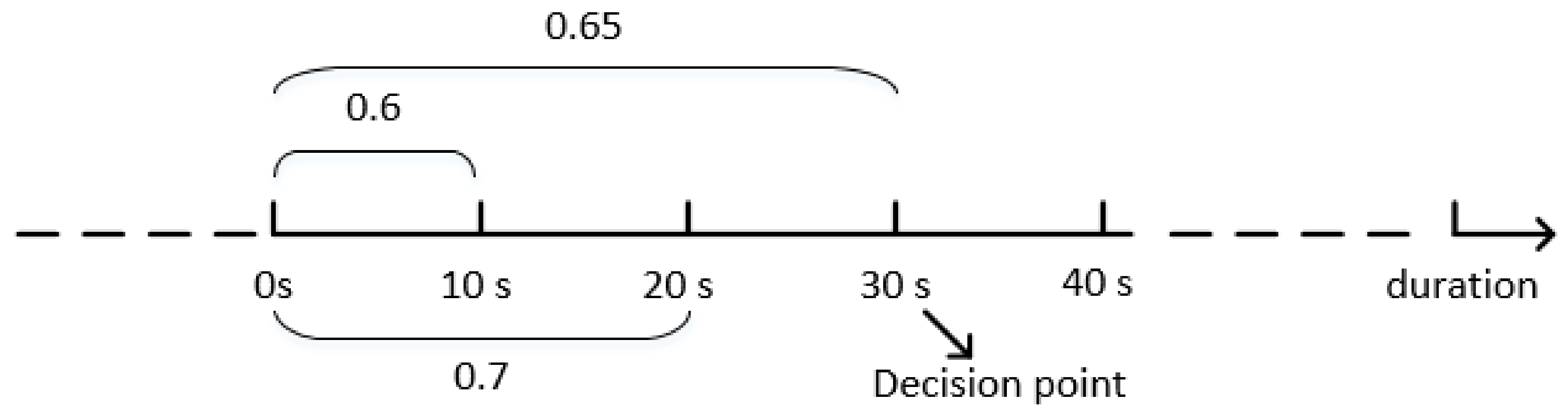
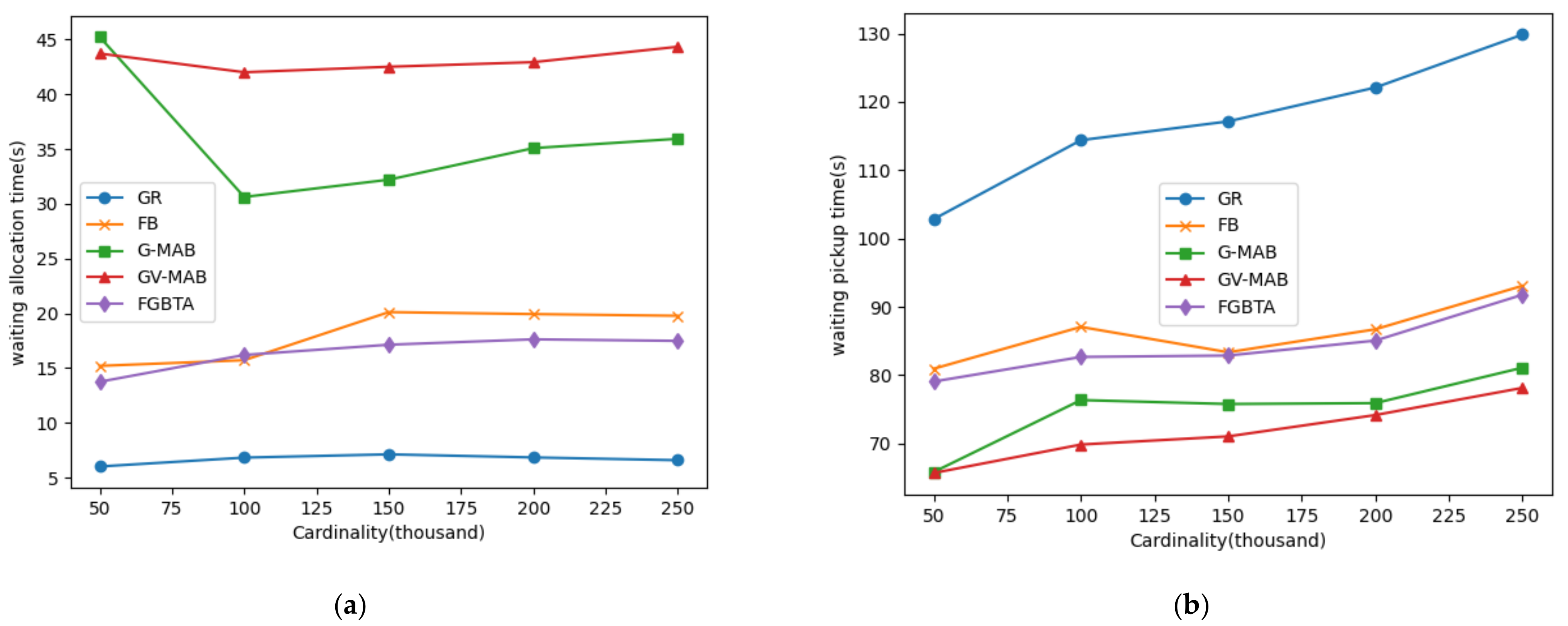
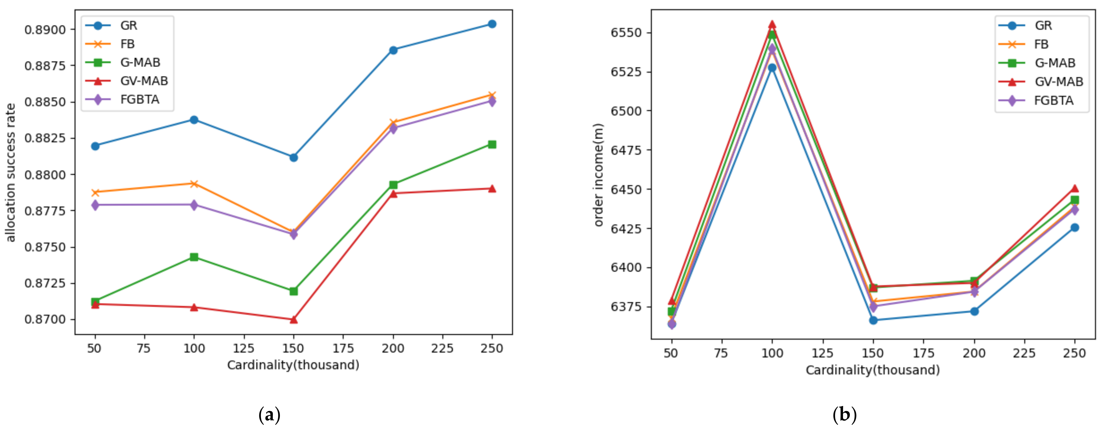
Table 1.
Mapping table of partial attributes required by spatial task.
| Data Mapping | Release Timestamp | Longitude of Task | Latitude of Task |
|---|---|---|---|
| properties from real data | pickup timestamp | pickup longitude | pickup latitude |
| required properties | release timestamp | longitude of the location | latitude of the location |
Table 2.
Mapping table of partial attributes required by worker.
| Data Mapping | Appear Timestamp | Longitude of Worker | Latitude of Worker |
|---|---|---|---|
| properties from real data | getting off timestamp | getting off longitude | getting off latitude |
| required properties | appear timestamp | longitude of the location | latitude of the location |
Table 3.
Setting of synthetic data parameters and algorithm parameters in concept drift experiment.
| Cardinality | (Radius) | (Duration) | (Interval) | (Exploration Rate) | (Adjustable Parameter) | |
|---|---|---|---|---|---|---|
| 100 K | 5 KM | 180 s | 10 s | 2 | 0.6 | 0.01 |
Table 4.
Setting of synthetic data parameters and algorithm parameters in duration experiment.
| Cardinality | ||||||
|---|---|---|---|---|---|---|
| 100 K | 5 KM | 50 s, 100 s, 150 s, 200 s, 250 s | 10 s | 2 | 0.6 | 0.01 |
Table 5.
Setting of synthetic data parameters and algorithm parameters in radius experiment.
| Cardinality | ||||||
|---|---|---|---|---|---|---|
| 100 K | 2 KM, 3 KM, 4 KM, 5 KM, 6 KM | 180 s | 10 s | 2 | 0.6 | 0.01 |
Table 6.
Setting of synthetic data parameters and algorithm parameters in exploration rate experiment.
Table 6.
Setting of synthetic data parameters and algorithm parameters in exploration rate experiment.
| Cardinality | ||||||
|---|---|---|---|---|---|---|
| 100 K | 5 KM | 180 s | 10 s | 2 | [0.1–1.0] | 0.01 |
Table 7.
Setting of synthetic data parameters and algorithm parameters in adjustable parameter experiment.
Table 7.
Setting of synthetic data parameters and algorithm parameters in adjustable parameter experiment.
| Cardinality | ||||||
|---|---|---|---|---|---|---|
| 100 K | 5 KM | 180 s | 10 s | 2 | 0.6 | [0.00–0.05] |
Table 8.
Setting of synthetic data parameters and algorithm parameters on real data sets.
| Cardinality | ||||||
|---|---|---|---|---|---|---|
| 50 K, 100 K, 150 K, 200 K, 250 K | 5 KM | 180 s | 10 s | 2 | 0.6 | 0.01 |
Publisher’s Note: MDPI stays neutral with regard to jurisdictional claims in published maps and institutional affiliations. |
© 2022 by the authors. Licensee MDPI, Basel, Switzerland. This article is an open access article distributed under the terms and conditions of the Creative Commons Attribution (CC BY) license (https://creativecommons.org/licenses/by/4.0/).
Share and Cite
MDPI and ACS Style
Jiao, Y.; Lin, Z.; Yu, L.; Wu, X. A Fine-Grain Batching-Based Task Allocation Algorithm for Spatial Crowdsourcing. ISPRS Int. J. Geo-Inf. 2022, 11, 203. https://doi.org/10.3390/ijgi11030203
AMA Style
Jiao Y, Lin Z, Yu L, Wu X. A Fine-Grain Batching-Based Task Allocation Algorithm for Spatial Crowdsourcing. ISPRS International Journal of Geo-Information. 2022; 11(3):203. https://doi.org/10.3390/ijgi11030203
Chicago/Turabian StyleJiao, Yuxin, Zhikun Lin, Long Yu, and Xiaozhu Wu. 2022. "A Fine-Grain Batching-Based Task Allocation Algorithm for Spatial Crowdsourcing" ISPRS International Journal of Geo-Information 11, no. 3: 203. https://doi.org/10.3390/ijgi11030203
Note that from the first issue of 2016, this journal uses article numbers instead of page numbers. See further details here.