
GeoAI for Large-Scale Image Analysis and Machine Vision: Recent Progress of Artificial Intelligence in Geography


School of Geographical Science and Urban Planning, Arizona State University, Tempe, AZ 85287-5302, USA
*
Author to whom correspondence should be addressed.
ISPRS Int. J. Geo-Inf. 2022, 11(7), 385; https://doi.org/10.3390/ijgi11070385
Submission received: 15 March 2022
/
Revised: 2 June 2022
/
Accepted: 7 July 2022
/
Published: 11 July 2022
(This article belongs to the Special Issue Upscaling AI Solutions for Large Scale Mapping Applications)
Abstract
:GeoAI, or geospatial artificial intelligence, has become a trending topic and the frontier for spatial analytics in Geography. Although much progress has been made in exploring the integration of AI and Geography, there is yet no clear definition of GeoAI, its scope of research, or a broad discussion of how it enables new ways of problem solving across social and environmental sciences. This paper provides a comprehensive overview of GeoAI research used in large-scale image analysis, and its methodological foundation, most recent progress in geospatial applications, and comparative advantages over traditional methods. We organize this review of GeoAI research according to different kinds of image or structured data, including satellite and drone images, street views, and geo-scientific data, as well as their applications in a variety of image analysis and machine vision tasks. While different applications tend to use diverse types of data and models, we summarized six major strengths of GeoAI research, including (1) enablement of large-scale analytics; (2) automation; (3) high accuracy; (4) sensitivity in detecting subtle changes; (5) tolerance of noise in data; and (6) rapid technological advancement. As GeoAI remains a rapidly evolving field, we also describe current knowledge gaps and discuss future research directions.
1. Introduction
GeoAI, or geospatial artificial intelligence, is an exciting research area which applies and extends AI to support geospatial problem solving in innovative ways. The research in AI, which stems from computer science, focuses on developing computer systems to gain machine intelligence to mimic the way the human perceives, reasons, and interacts with the world and with each other [1]. Although the field of AI has experienced highs and lows in the past decades, it has recently gained tremendous momentum because of breakthrough developments in deep (machine) learning, immense available computing power, and the pressing needs for mining and understanding big data. With little doubt, AI has become the new space race in the 21st century because of its great importance in boosting the national economy, ensuring homeland security, providing rapid emergency response, and empowering a competitive workforce. AI technologies are widely applied in industry and science [2], notably in chemistry [3], mathematics [4], medical science [5], psychology [6], neuroscience [7], astronomy [8], and beyond.
The upward trend of research adopting AI does not stop with geography. In fact, geography is one of the fields which has made serious use of AI, having adopted it in the early days. Because of the interdisciplinary nature of its research agenda, Geography has the natural advantage of embracing new theories, methods, and tools from other disciplines. Back in the 1990s, Openshaw and Openshaw [9] published a book on “Artificial Intelligence in Geography”, which introduced AI techniques and methods, such as expert systems, neural networks, fuzzy system, and evolutional computation, which were state-of-the-art at the time, as well as their applications in Geography. Besides becoming the landmark reference for AI in Geography, it also drove discussion and criticism regarding the combination of the two fields and the scientific properties of AI [10]. Although some of the concerns, such as AI interpretability and the lack of “theory”, remain valid today, AI research has advanced so dramatically in recent years that it has evolved from modeling formal logic to exploration of the more data-driven, deep learning-based research landscape, which is in high demand as a powerful way to analyze ever-increasing big data.
Geography is becoming a field of big data science. In the domain of physical geography, global observation systems, such as operational satellites, which provide continued monitoring of the environment, atmosphere, ocean, and other earth system components, are producing vast amount of remote sensing imagery at high or very high spatial, temporal, and spectral resolutions. The distributed sensor network systems deployed in cities are also collecting real-time data about the status of physical infrastructures and movement of people, vehicles, and other dynamic components of a (smart) city [11]. For social applications, the prevalent use of location-based social media, GPS-enabled handheld devices, various Volunteer Geographic Information (VGI) platforms, and other “social sensors” have fostered the creation of massive information about human mobility, public opinion, and people’s digital footprints at scale. Besides being voluminous, these data sets contain a variety of formats, from structured geo-scientific data to semi-unstructured metadata to unstructured social media posts. These ever-increasing geospatial resources provide added value to existing research by allowing us to answer questions at a scale which was not previously possible. However, it also poses significant challenges for traditional analytical methods which were designed to handle small data sets of good quality [12]. To fully utilize the scientific value of geospatial big data, geographers started to switch gears toward data-driven geography, which relies on AI and machine learning to enable the discovery of new geospatial knowledge.
The term “GeoAI” was first coined at the 2017 ACM SIGSPATIAL conference [13]. It was then quickly adopted by high-tech companies, such as Microsoft and Esri, to refer to their enterprise solutions that combined location intelligence and artificial intelligence. Researchers frequently use this term when their research involves data mining, machine learning, and deep learning, a recent advance in AI. Here we define GeoAI as a new transdisciplinary research area that exploits and develops AI for location-based analytics using geospatial (big) data. Figure 1 depicts a big picture view of GeoAI. It integrates AI research with Geography, which is the science of place and space. If we agree that AI is about the development of machine intelligence that can reason like humans, GeoAI, which is the nexus of AI and Geography, aims at developing the next-generation machines that possess the ability to conduct spatial reasoning and location-based analytics, as do humans, with the aid of geospatial big data. Under the umbrella of AI, machine learning and other data-driven algorithms, which can mine and learn from massive amount of data without being explicitly programmed, have become cornerstone technology. And deep learning, as a subset of machine learning, represents the breakthrough development that advances machine learning from a shallow to a deep architecture allowing the modeling and extraction of complex patterns via the utilization of artificial neural networks. To better fuse AI and Geography and establish GeoAI as a research discipline that will last, there needs to be a strong interlocking of the two fields. Geography offers a unique standpoint for understanding the world and society through the guidance of well-established theories, such as Tobler’s first law of Geography [14] and the second law of Geography [15]. These theories and principles will expand current AI capabilities toward spatially-explicit GeoAI methods and solutions [16,17] so that AI can be more properly adapted to the geospatial domain. Its research territory can also be enlarged by integrating with geospatial knowledge and spatial thinking.
Just like any emerging topic that sits across multiple disciplines, the development of GeoAI has been undergoing three phases: (1) A simple importing of AI into Geography. In this phase, research is more exploratory and involves the direct use of existing AI methods by geospatial applications. The goal is really to test the feasibility in combining the two fields. (2) AI’s adaptation through methodological improvement. This phase identifies the challenges of applying and tailoring AI to help better solve various kinds of geospatial problems. (3) The exporting of geography-inspired AI back to computer science and other fields. In this phase, we will gain an in-depth knowledge of how AI works and how it can be applied, and we will focus on building new AI models by injecting spatial principles, such as spatial autocorrelation and spatial heterogeneity, for more powerful, general-purpose AI that can be adopted by many disciplines. Phase 2 and Phase 3 will build the theoretical and methodological foundation of GeoAI.
It is also important to discern the methodological scope of GeoAI. Researchers today frequently use GeoAI when their geospatial studies apply data mining, machine learning, and other traditional AI methods. Regression analysis and other shallow machine learning methods have existed for many decades, but it is deep machine learning techniques, such as the convolutional neural network (CNN), that have gained the interest of AI researchers and fostered the growth of the GeoAI community. Therefore, while a broad definition of GeoAI techniques shall include more traditional AI and machine learning methods, its core elements shall be deep learning and other more recent advances in AI in which important learning steps, such as feature selections, are done automatically rather than manually. In addition, methods should be scalable in processing geospatial big data.
This paper aims to provide a review of important methods and applications in GeoAI. We first reviewed key AI techniques including feed-forward neural networks, CNNs, Recurrent Neural Networks (RNNs), long- and short-term memory (LSTM) neural networks, and transformer models. These models represent some of the most popular neural network models that dominate modern AI research. We organize the review around the use of geospatial data. As the literature of GeoAI is growing so rapidly, every topic cannot be covered in a single paper. To ensure both depth and breadth of this review, we give preference to groundbreaking work in AI and deep learning, and seminal works that represent the most important milestones in expanding and applying AI to the geospatial domain. We also centered our review on research that leverages novel machine learning techniques, in particular deep learning, while touching on shallow machine learning methods for a comparative analysis. We hope this paper will serve as a fundamentally orienting paper for GeoAI that summarizes the progress of GeoAI research, particularly in tasks geospatial image analysis and machine vision.
The reminder of this paper is organized as follows: Section 2 briefly describes different types of geospatial big data, particularly structured and image data. Section 3 introduces popular methodology in GeoAI research. Section 4 reviews different applications that GeoAI enables. Section 5 summarizes the paper and discusses ways forward for this exciting research area.
2. Geospatial Big Data for Image Analysis and Mapping
- Remote sensing images
Remote sensing imagery is one of the most important and widely used data sources in Geography. It involves information extracted from the Earth’s surface and contains not only human-made features but also natural features. Recent advances in large-scale earth observation and unmanned aviation vehicles (UAVs) result in huge advantages to using remote sensing imagery, such as satellite and drone images, to support applications across multiple geographical scales [18].
- Google Street View
The recent availability of street-level imagery from high-tech companies, such as Google and Tencent, has become a useful way to derive information about the world without stepping into it [19]. In contrast to remote sensing imagery, street view data provide more human-centric observations which contain not only the physical environment but also the social environment [20], as well as other fine-grained information related to cities, such as human mobility and socioeconomic trends [21]. As more and more street view images are generated and machine learning techniques continue to be developed, street image data are being increasingly leveraged.
- Geo-scientific data
The study of Earth’s physical phenomena is important for the human condition. From understanding to predicting, for example, the weather and flooding, to environmental monitoring, geospatial research not only protects people from exposure to extreme events, but also ensures sustainable development of society. There are generally two types of data used in the research of Earth’s systems: sensor data and simulation data. Sensor data, such as temperature and humidity, became widely available because of advancements in hardware technology [16,22]. On the other hand, simulation data are the outputs of models which assimilate information about the Earth’s atmosphere, oceans, and other systems. Both types of data are structured, but they differ from natural images and therefore lead to unique challenges. For example, they are usually high-dimensional and in massive quantities. Their size can be in tera- to peta-byte levels with dozens of geophysical or environmental variables, while an ordinary image dataset is normally at gigabyte scale and has only three channels (RGB). In addition, different sensors may have different spatial and temporal resolutions, increasing the challenges for data integration. To address these challenges, various studies with different applications have been developed.
- Topographic map
Topographic maps contain fine-granule details and quantitative representation of the Earth’s surface and its features, both natural and artificial. On such a map, the features are labeled, and elevation changes are annotated. Topographic maps integrate multiple elements (e.g., features differentiated by color and symbols, labels for feature name, and contour lines showing the terrain changes) to provide a comprehensive view about the terrain. The U.S. Geological Survey is well known for creating the topographic map named U.S. Topo that covers the entire U.S. [23].
Compared to the use of other datasets, topographic mapping is often a primary focus of the government, such as by the United States Geological Survey (USGS). Usery et al. [24] has provided a thorough review of relevant GeoAI applications in topographic mapping, so we will focus on reviewing application using remote sensing images, street view images, and geoscientific data.
3. Methodology
In this review, we categorized articles into three types based on their use of data: remote sensing imagery, street view imagery, and geoscientific data. Each has its own characteristics and processing routines, so the corresponding techniques and methodologies vary. Based on data characteristics, we adopted different strategies for selecting and reviewing the literature. Remote sensing imagery has been used since 1960s or earlier, hence, various techniques have been developed and applied to such data before machine learning and GeoAI have become mainstream techniques, resulting in a large body of works in the area of remote sensing image analysis. To conduct this review, we categorized relevant publications by their tasks, e.g., image classification and object segmentation. Besides introducing applications (e.g., land use classification) of each task, we also describe the use of conventional methods and the more cutting-edge GeoAI/deep learning methods, as well as summarize their differences in a table. For conventional methods, we selected publications with a high number of citations from Google Scholar (~top 40 articles returned using search keywords, such as “remote sensing image classification”) in each task area. For deep learning methods, we selected breakthrough publications in terms of new model development in computer science based on our best knowledge and citation count from Google Scholar. Applications of deep learning methods in remote sensing image analysis are reviewed in more recent literature (2019–2022) to keep the audience informed on the recent progress in this area.
The second focused area of the review is street view imagery, the use of which has a relatively short history compared to remote sensing imagery. Techniques for collecting street view imagery started in 2001 and the data became available for research at around 2010. Because it is a new form of data, there are fewer studies in this area than for remote sensing imagery. Research that can benefit from street view imagery normally involves human activities and urban environmental analysis, which traditionally require in-person interviews or on-site examinations. Street view imagery offers a new way for obtaining information at a large-scale and GeoAI and deep learning enable automated information extraction from such data to reduce human effort and enable large-scale analysis. Here, we categorize our review by applications (e.g., quantification of neighborhood properties) and discuss how GeoAI and deep learning can support such applications. As most recent research in this area has been published after 2017, we did not specify the time range when doing the survey.
The third focus area includes the GeoAI applications of geo-scientific data. Compared to data in the other two categories, geo-scientific data are much more complex in structure and are heterogeneous when data come from different geoscience domains. Because of this, methods used to analyze such data also show large variances even though they are performing the same tasks in different applications. Therefore, we categorized publications by domain applications. Traditionally, scientists rely heavily on physics-based models to understand geophysical phenomena using geo-scientific data. As such, data are highly structured and can be represented as image-type data. In the recent years, GeoAI and deep learning have been increasing applied to derive new insights from these data and they be used as a complementary approach to the physics-based models. The review of traditional approaches or tools is based on their popularity and widespread adoption in large-scale study and forecasting, and the review of more recent deep learning applications is provided for comparison purposes.
4. Survey of Popular Neural Network Methods: From Shallow Machine Learning to Deep Learning
In this section, we review popular and widely used AI methods, particularly the deep learning models. Five major neural network architectures are introduced, including Fully Connected Neural Network (FCN) [25], which is a foundational component in many deep learning based neural network architectures; Convolutional Neural Network (CNN) [17] for “spatial” problems; Recurrent Neural Network (RNN) [26] and LSTM (Long, Short-Term Memory) Neural Network model [26,27] for time sequence; as well as transformer models [28], which have been increasingly used for vision and image analysis tasks. These methods also serve as the foundation for developing the research agenda for methodological development in GeoAI.
4.1. Fully Connected Neural Network (FCN)
Traditional artificial neural network models are the foundation of cutting-edge neural network architectures. For instance, the feed-forward neural network (Figure 2a) involves the placement of artificial neurons, each representing an attribute or a hidden node, in multiple layers. Each neuron in the previous layer has a connection with every neuron in the next layer. This type of neural network is also called a fully connected neural network and is capable of identifying non-linear relationships between the input and the output. However, they suffer from two major limitations: (1) the need to manually define the number of the input nodes, or independent variables, which are also important attributes that help to make final classification and (2) to gain a good predictive capability, the network needs to stack multiple neural network layers in order to learn a complex, non-linear relationship between the independent (the input) and dependent variable (the output). The learning process for such a complicated network is often very computationally intensive, and with its use, it is also difficult to converge on an optimal solution. To address these challenges, newer parallelly processing neural network models have been developed, one of which is CNN. Note that traditional models, particularly the fully connected neural networks, remain an essential component in many deep learning architectures for classification. The manual feature extraction is replaced by automated processing achieved by newer models. And CNN is one of them.
4.2. Convolutional Neural Network (CNN)
CNN is a breakthrough in AI that enables machine learning with big data and parallel computing. The emergence of CNN (Figure 2b) resolves the high interdependency among artificial neurons in an FCN by applying a convolution operation, which uses a sliding window to calculate the dot product between different parts (within the sliding window) of the input data and the convolution filter of the same size. The result is called a feature map and its dimensions depend on the design of the convolution filter. A convolution layer is often connected with a max-pooling layer, which conducts down-sampling to select the maximum value in the non-overlapping 2 by 2 subareas in the feature map. This operation ensures the prominent feature is preserved. At the same time, it reduces the size of the feature map, thus lowering computation cost. After stacking multiple CNN layers, the low-level features which are extracted at the first few layers can then be composed semantically to create high-level features which can better discern an object from others. CNN can be viewed as a general-purpose feature extractor.
Depending on the different types of data that a CNN can take, it can be categorized as 1D CNN, 2D CNN, or 3D CNN. The 1D CNN applies a one-dimensional filter which slides along the 1D vector space; it is therefore suitable for processing sequential data, such as natural language text or audio segment. The 2D CNN, in comparison, applies a filter with size at x × y × n, in which x and y are the dimensions for the 2D convolution filter and n is the number of filters applied to extract different features, e.g., horizontal edges and vertical edges. The 2D filter slides only in the spatial domain. When expanding 2D (image) data into 3D volume data, such as video clips in which the third z dimension is the temporal dimension, the filter is correspondingly in 3D and slides in all x, y, and z directions.
After feature extraction, the model can be further expanded for various applications. For image processing and computer vision, the model can be connected to a fully connected layer for image-level classification, or to a region proposal network for object detection or segmentation. For natural language processing (NLP), the text documents can be represented and converted as matrices of word frequency and then CNN can be leveraged for topic modeling and other text analysis tasks, such as semantic similarity measurement. For processing 3D data with properties of both space and time, or 3D LiDAR data depicting 3D objects, 3D CNN can be leveraged for motion detection or detection of 3D objects. Because of its outstanding ability in extracting discriminative features and its novel strategy in breaking the global operation into multiple local operations, a CNN gains much improved performance in both accuracy and efficiency compared to traditional neural networks. It therefore becomes a building block for many deep learning models.
4.3. Recurrent Neural Network (RNN)
While CNNs have found widespread application, particularly in computer vision and image processing, they are limited in the types of problems they can solve. Because a regular CNN takes a fixed-size input and created a fixed-size output, it cannot process a series of data with interdependency among the datasets at different time slices. To this end, RNN has been developed to add a hidden state to capture the context between the previous input and the output. In other words, the output is not only a function with an input at ‘time’ i (if we consider the dependency of the series of input is time), it also depends on the contextual information provided by the hidden state at time i − 1. Figure 2c illustrates a typical architecture of an RNN. Each hidden state node leverages a feed-forward NN, as shown in Figure 2a with two output nodes. In the example in Figure 2c, the RNN contains a chain of three hidden states (h (0) is a predefined hidden state). That means during the training, the RNN will learn to make a decision based on its current input and the hidden state memorizing contextual information from two previous states.
Similar to 2D CNN, which uses the same filter to perform convolution at different sub-regions of 2D data, the RNN also uses the same weights in <, , > for the calculation at all recurrent states. The architecture of an RNN can be altered according to different application needs. For instance, a one-to-many model (one input, many outputs) can be used for caption learning from an image; a many-to-one model can be used for action classification from a video clip; and a many-to-many model can be used for language translation. Finally, a one-to-one RNN model will be simplified into a feed-forward neural network. By adding bidirectional connections between input, hidden, and output nodes, a bi-directional RNN can be created to capture the context from not only previous states but also future states.
An RNN model can also evolve to a deep RNN by increasing the length of the hidden states chain by adding depth to the transition between input to hidden, hidden to hidden, and hidden to output layers [29]. It is generally recognized that a deep RNN performs better than a shallow RNN because of the ability of a deep RNN to capture long-term interdependencies within the input series.
4.4. Long- Short-Term Memory (LSTM)
Deep RNN can capture long-term memory, and shallow RNN captures short-term memory in the input series. However, the memory they can capture is only at a fixed length. This limits an RNN’s ability to dynamically capture events with different temporal rhythms, negatively affecting its prediction accuracy. LSTM models are developed to address this limitation. As its name suggests, LSTM has the ability to flexibly determine whether and when short-term memory or long-term memory is more important in making decisions. It achieves this by introducing a cell state in addition to the hidden states in regular RNNs. The cell states preserve the long-term memory about event patterns, and the hidden states contain the short-term memory (Figure 2d). To determine which part of the memory should be considered to enable more accurate temporal pattern recognition, LSTM also introduces three gates: an input gate, a forget gate, and an output gate. The input gate determines the amount of input information from the previous state that should flow into the current state in an iterative training process. In other words, it will determine how much new information will be used. A forget gate decides which part of the memory is less important and therefore should be forgotten. And the output gate decides how to combine newly derived information with that filtered from memory to make an accurate prediction about a future state.
Because of its ability to capture long-term dependencies, LSTM has been widely used for time sequence predictions. For instance, a time series of satellite images can serve as the input of LSTM and the model predicts how land use and land cover will change in the future [30]. Depending on the application, LSTM input could be original time sequence data, or a feature sequence extracted using CNN models mentioned above. One interesting application of LSTM in image analysis is its adoption for object detection [31]. Although a single image does not contain time variance, the 2D image can be serialized into 1D sequence data by a scan order, such as row priming. In an object detection application, although the 2D objects will be partitioned into parts after the serialization, LSTM will be able to “link” the 1D subsequences belonging to the same object and make proper predictions because of its ability to capture the long-term dependency. When LSTM is used in combination with new objective functions, such as CTC (Connectionist Temporal Classification), it would be able to predict on a weak label instead of a per-frame label [27]. This significantly reduces labeling cost and increases the usability of such models in data-driven analysis.
LSTM can also be used to process text documents to predict the forthcoming text sequence or perform speech segmentation. These applications, however, are not the focus of this paper.
4.5. Transformer
Another very exciting neural network architecture is transformer, which was developed by the Google AI team in 2017 [28]. It is based on an encoder and decoder architecture and has the ability to transform an input sequence to an output sequence. This is also known as sequence-to-sequence learning. Transformers have been increasingly used in natural language processing, machine translation, question answering, and tasks related to processing sequential data. Different from other sequential data processing models, such as an RNN, a transformer model does not contain recurrent modules, meaning that the input data do not need to process sequentially, instead they can be processed in batch. A core concept that enables this batch or parallel processing is an attention mechanism. Once an input sequence is given, e.g., a sequence of words, the self-attention module will first derive the correlations between all word pairs. For a given word, this means calculating a weight to know how this word is influenced by all the other words in the sequence. These weights will be incorporated into the following computation to create a high-dimensional vector to represent each word (element) in the input sequence. This is also known as the encoding progress. Instead of directly using the raw data as input, the encoder will first conduct input embedding to represent the elements of the input sequence numerically. In addition, a positional encoding is introduced to notify the self-attention module the position of each element in the input sequence. A feed-forward layer is connected with the self-attention module for dimension translation of the encoded vector so it fits better with the next encoder or decoder layer. The encoder runs iteratively to derive the high-dimensional vector that can best represent the semantics of each element in the input sequence.
The decoder (Figure 2e) has an architecture similar to that of the encoder. It takes the output sequence as input (during the training process) and performs both position encoding and embedding on top of the sequence. The embedded vectors are then sent to the attention module. Here, the attention module is called masked attention because the calculation of attention values is not based on all the other elements in the sequence. Instead, because the decoder is used for predicting the next element in the sequence, the attention calculation for each element takes only those coming before it into the sequence rather than all elements in the sequence. This module is therefore called masked self-attention. Besides this module, the decoder also introduces a cross attention module that takes the embedded input sequence and already predicted output sequence to jointly make predictions about the upcoming element. The predictions could be single or multiple labels for a classification problem (i.e., to predict who the speaker is, given a piece of speech sequence), it can also be a non-fixed length vector for machine translation (i.e., from one language to another, or from speech to text).
Besides applications in natural language processing, transformer models have been increasingly used for image analysis and other machine vision tasks. The CNN focuses its attention on a smaller local window (a.k.a., a smaller receptive field) through its convolutional neural network. Comparatively, transformers can dynamically determine the size of a receptive field and can achieve similar or even better performance than CNN [32]. In recent years, Vision Transformers (ViTs) have been considered as the “Roaring 20s” and they surpass CNN models as the state-of-the-art image classification models. However, for more challenging image analysis tasks, such as object detection and semantic segmentation, CNNs still show more favorable performance than transformers [33].
In summary, the revolutionary development of new neural network models, particularly CNN, and LSTM and transformer models, have unique advantages in processing sequence and/or image data. They each therefore play an indispensable role in domain applications. Other machine learning models, such as deep reinforcement learning, generative adversarial network (GAN), and self-supervised learning, are high-level algorithms built upon these foundational neural network structures, and their applications for image and vision tasks will be reviewed in the next section.
5. Applications
5.1. Remote Sensing Image Analysis
To extract information from imagery, traditional approaches often employ image processing techniques, such as edge detection [34,35], and hand-crafted feature extraction, such as SIFT (Scale-Invariant Feature Transform) [36], HOG (Histogram of Oriented Gradients) [37], and BoW (Bag of Words) [38]. These methods require some or more prior knowledge and might not be adaptable to different application scenarios. Recently, CNN has proved to be a strong feature descriptor because of its superior ability to learn representations directly from the original imagery with little or no prior knowledge [39]. Much of current state-of-the-art work has adopted CNN as feature extractors, for example, for object detection [40] and sematic segmentation [41]. However, most of this work uses natural scene images taken from an optical camera and more challenges exist when the models are applied to remote sensing imagery. For instance, such data provide only a roof view of target objects, and the area coverage is large, but the objects are usually small. Therefore, the available information of objects is limited, not to mention issues of rotation, scale, complex background, and object-background occlusions. Therefore, expansion and customization are often needed when utilizing deep learning models with remote sensing imagery.
Next, we introduce a series of applications applying GeoAI and deep learning to remote sensing imagery. Table 1 summarizes these applications, methods used, and limitation of traditional approaches.
- Image-level classification
Image-level classification involves the prediction of content in a remotely sensed image with one or more labels. This is also known as multi-label classification (MLC). MLC can be used for predicting land use or land cover types within a remotely sensed image, it can also be used to predict the features, either natural or manmade, to classify different types of images. In the computer vision domain, this has been a very popular topic and has been a primary application area for CNN. Large-scale image datasets, such as ImageNet, were developed to provide a benchmark for evaluating the performance of various deep learning models [42]. The past few years have witnessed continuous refinement of CNN models to be utilized for MLC, particularly with remote sensing imagery. Examples include (1) the groundbreaking work on AlexNet [43], which was designed with five convolutional layers for automated extraction of important image features to support image classification, and (2) VGG [44], which stacks tens of convolutional layers to create a deep CNN. Besides the convolutional module, another milestone development in CNN is the inception module, which applies convolutional filters at multiple sizes to extract features at multiple scales [45]. In addition, the enablement of residual learning in ResNet [46] allows useful information to pass from shallow layers to not only their immediate next layer but also to much deeper layers. This advance avoids problems of model saturation and overfitting that traditional CNN encounters. Although different optimization techniques, such as dense connection and fine-tuning, are applied to further improve the model performance [47,48,49,50], they rest upon these building block and milestone developments of these CNN models.
In remote sensing image analysis, CNNs and their combination with other machine learning models are leveraged to support MLC. Kumar et al. [51] compared 15 CNN models and found that Inception-based architectures achieve the overall best performance in MLC of remotely sensed images. The UC-Merced land use dataset is used in this study [52]. Several CNN models also beat solutions using graph neural network (GNN) models for image classification on the same dataset [53]. These models benefit from transfer learning, which involves the training of the models on the popular ImageNet dataset to learn how to extract prominent image features and fine tune them based on the remote sensing images in the given tasks. Recent work by Li et al. [54] also shows that the combined use of CNN with GNN could in addition capture spatio-topological relationships, and therefore contributes to a more powerful image classification model.
- Object detection
Object detection aims to identify the presence of objects in terms of their classes and bounding box (BBOX) locations within an image. There are in general two types of object detectors: region-based and regression-based. Region-based models treat object detection as a classification problem and separate it into three stages: region proposal, feature extraction, and classification. The corresponding deep learning studies include OverFeat [55], Faster R-CNN [56], R-FCN [57], FPN [58], and RetinaNet [59]. Regression-based models directly map image pixels to bounding box coordinates and object class probabilities. Compared to region-based frameworks, they save time in handling and coordinating data processing among multiple components and are desirable in real-time applications. Some popular models of this kind include YOLO [60,61,62,63], SSD [64], RefineDet [65], and M2Det [66].
Object detection can find a wide range of applications across social and environmental science domains. It can be leveraged to detect natural and humanmade features from remote sensing imagery to support environmental management [67], urban planning [68], search and rescue operations [69], and the inspection of living conditions of underserved communities [70]. It has also found application in the aviation domain where satellite images are used to detect aircraft which can help track aerial activities, as well as other environmental factors, such as air and noise pollution owing to said traffic [71]. CapsNet [72] is a framework that enables the automatic detection of targets in remote sensing images for military applications. Li and Hsu [73] extends Faster R-CNN [56] to enable natural feature identification from remote sensing imagery. The authors evaluated performance of multiple deep CNN models and found that very complex and deep CNN models will not always yield the best detection accuracy. Instead, CNN models should be carefully designed according to characteristics of the training data and complexity of objects and background scenes. Other issues and strategies that may improve object detection performance, such as rotation-sensitive detection [74,75,76,77,78,79], proposal quality enhancement [80,81,82,83], weakly-supervised learning [27,84,85,86,87], multi-source object detection [88,89], and real-time object detection [90,91,92], also have been increasingly studied in recent years [93].
- Semantic segmentation
Semantic segmentation involves classifying individual image pixels into a certain class, resulting in the division of the entire image into semantically varied regions representing different objects or classes. It is also a kind of pixel-level classification. Several methods have been developed to support semantic segmentation. For instance, region-based segmentation [94,95] separates the pixels into different classes based on some threshold values. Edge-based segmentation [96,97] defines the boundary of objects by detecting edges where the discontinuity of local context appears. Clustering-based segmentation [98,99] divides the pixels into clusters based on certain criteria, such as similarity in color or texture. Recent neural network-based segmentation methods bring new excitement to this research. These models learn an image-to-image mapping from pixels to classes, which is different from image-to-label mapping, such as for image-level classification. Because it requires a finer granularity analysis of the image, semantic segmentation is also a more time consuming and challenging task in image analysis. To achieve this, most of the neural network-based models utilize an encoder/decoder-like architecture, such as U-Net [100], FCN [101], SegNet [102], DeepLab [103,104,105], AdaptSegNet [106], Fast-SCNN [107], HANet [108], Panoptic-deeplab [109], SegFormer [110], or Lawin+ [111]. The encoder conducts feature extraction through CNNs and derives an abstract representation (also called a feature map) of the original image. The decoder takes these feature maps as input and performs deconvolution to create a semantic segmentation mask.
Semantic segmentation is frequently employed in geospatial research to identify significant areas in an image. For example, Zarco-Tejada et al. [112] developed an image segmentation model to separate crops from background to conduct precision agriculture. Land use and land cover analysis detect land cover types and their distributions in an image scene. The automation of such an analysis is extremely helpful for understanding the evolution of urbanization, deforestation, and other urban and environmental changes. Many studies have been conducted to address the challenges of segmentation with remote sensing imagery. For example, Kampffmeyer et al. [113] proposed strategies, such as patch-based training and data augmentation, to solve the issue of small objects tending to be ignored in segmentation tasks to achieve better overall prediction accuracy. Fitoka et al. [114] developed a segmentation model to use remote sensing imagery to map global wetland ecosystems for water resource management and their interactions with other earth system components. Mohajerani and Saeed [115] used image segmentation to detect and remove clouds and cloud shadows from images to reduce error in biophysical and atmospheric analyses.
Road extraction and road width estimation is another interesting challenge that can be solved using segmentation. The idea is to combine remotely sensed images with monocular images taken at street level and other geospatial data to build a foundational infrastructure dataset for transportation research [116]. There are also techniques developed to enhance image segmentation to achieve real-time processing [117,118], the successful use of multi-spectral data [119,120,121], and the detection of small object instances [122,123,124,125].
- Height/depth estimation of 3D object from 2D images
Understanding 3D geometry of objects within remotely sensed imagery is an important technique to support varied research, such as 3D modeling [126], smart cities [127], and ocean engineering [128]. In general, two types of information can be extracted from remote sensing imagery about an 3D object: height and depth. LiDAR data and its derived digital surface model (DSM) data could support the generation of a height or depth map to provide such information. However, derivation of LiDAR data is often expensive, so it is difficult to achieve global coverage. In comparison, the development of satellites has allowed remote sensing imagery to become a globally achievable and low-cost alternative. There are generally two methods in the computer vision field to extract height/depth from 2D images: monocular estimation and stereo matching. The aim of monocular estimation is to map the image context to a real-world height/depth value from a single image. Because the depth/height of a particular location relates not only to the local features but also its surroundings, a probabilistic graphical model is often used to model such relations. For example, Saxena et al. [129] used a Markov Random Field (MRF) model to map the appearance features relating to a given point to a height value. Features can also be of various forms, such as hand-crafted features [129], semantic labels [130,131,132,133,134], and CNN-extracted features [135,136,137,138]. Eigen et al. [139] used two CNNs to extract information from global and local views, respectively, and later combine them by estimating a global depth structure and refining it with local features. This work was later improved by Eigen and Fergus [140] to predict depth information using multi-scale image features extracted from a CNN. D-Net [141] is a new generalized network that gathers local and global features at different resolutions and helps obtain depth maps from monocular RGB images.
In stereo matching, a model calculates height/depth using triangulation from two consecutive images and the key task is to find corresponding points of the two images. Scharstein and Szeliski [142] reviewed a series of two-frame stereo correspondence algorithms. They also provided a testbed for the evaluation of stereo algorithms. Machine learning techniques have also been applied in the stereo case and this often leads to better results by relaxing the need for careful camera alignment [143,144,145]. For estimating height/depth, images remotely sensed and from the field computer vision have different characteristics and offer different challenges. For example, remotely sensed images are often orthographic, containing limited contextual information. Also, they usually have limited spatial resolution and large area coverage but the targets for height/depth prediction are tiny. To address these issues, Srivastava et al. [146] developed a joint loss function in a CNN which combines semantic labeling loss and regression loss to better leverage pixel-wise information for fine-grained prediction. Mou and Zhu [135] proposed a deconvolutional neural network and used DSM data to supervise the training process to reduce massive manual effort for generating semantic masks. Recently, newer approaches, such as semi-global block matching, have been developed to tackle more challenging tasks, such as matching regions containing water bodies, for which accurate disparity estimation is difficult to identify because of the lack of texture in the images [147].
- Image super resolution
The quality of images is an important concern in many applications, such as medical imaging [148,149], remote sensing [150], and other vision tasks from optical images [151,152]. However, high-resolution images are not always available, especially those for public use and that cover a large geographical region, due partially to the high cost of data collection. Therefore, super resolution, which refers to the reconstruction of high-resolution (HR) images from a single or a series of low-resolution (LR) images, has been a key technique to address this issue. Traditional super resolution approaches can be categorized into different types, for example, the most intuitive method is based on interpolation. Ur and Gross [153] utilized the generalized multichannel sampling theorem [154] to propose a solution to obtain HR images from the ensemble of K spatially shifted LR images. Other interpolation methods include iteration back-projection (IBP) [155,156] and projection onto convex sets (POCS) [157,158]. Another type relies on statistical models for learning statistically a mapping function from LR images to HR images based on LR-HR patch pairs [159,160]. Others are built upon probability models, such as Bayesian theory or Markov random field [161,162,163,164]. Some super resolution methods operate in a different way than the image domain. For instance, images are transformed into a frequency domain, reconstructed, and transformed back to images [165,166,167]. The transformation is done by certain techniques, such as Fourier transformation (FT) or wavelet transformation (WT).
Recently, the development of deep learning has contributed much to image super-resolution research. Related work has employed CNN-based methods [168,169] or Generative Adversarial Network (GAN)-based methods [170]. Dong et al. [168] utilized a CNN to map between LR/HR image pairs. First, LR image are up-sampled to the target resolution using bicubic interpolation. Then, the nonlinear mapping between LR/HR image pairs are simulated by three convolutional layers, which represent feature extraction, non-linear mapping, and reconstruction, respectively. Many similar CNN-based solutions have also been proposed [169,171,172,173,174,175] and they differ in network structures, loss functions, and other model configurations. Ledig et al. [170] proposed a GAN-based image super resolution method to address the issue of generating less realistic images by commonly used loss functions. In a regular CNN, mean squared error (MSE) is often used as the loss function to measure the differences between the output and the ground truth. Minimizing this loss will also maximize the evaluation metric for a super-resolution task—the peak signal-to-noise ratio (PSNR). However, the reconstructed images might be overly smooth since the loss is the average of pixel-wise differences. To address this issue, the authors proposed a perceptual loss that encourages the GAN to create a photo-realistic image which is hardly distinguishable by the discriminator. Besides panchromatic images (PANs), dealing with hyperspectral images (HSIs) is more challenging due to difficulties collecting HR HSIs. Therefore, studies focusing on reconstruction of HR HSIs from HR PANs and LR HSIs [176,177,178,179,180] have also been reported. In more recent years, approaches, such as EfficientNet [181], have been proposed to enhance Digital Elevation Model (DEM) images from LR to HR by increasing the resolution up to 16 times without requiring additional information. Qin et al. [182] proposed an Unsupervised Deep Gradient Network (UDGN) to model the recurring information within an image and used it to generate images with higher resolution.
- Object tracking
Object tracking is a challenging and complex task. It involves estimating the position and extent of an object as it moves around a scene. Applications in many fields employ object tracking, such as vehicle tracking [183,184], automated surveillance [185,186], video indexing [187,188], and human-computer interaction [189,190]. There are many challenges to object tracking [191], for example, abrupt object motion, camera motion, and appearance change. Therefore, constraints, such as constant velocity, are usually added to simplify the task when developing new algorithms. In general, three stages compose object tracking: object detection, object feature selection, and movement tracking [192]. Object detection identifies targets in every video frame or when they appear in the video [56,193]. After detecting the target, a unique feature of the target is selected for tracking [194,195]. Finally, a tracking algorithm estimates the path of the target as it moves [196,197,198]. Existing methods differ in their ways of object feature selection and motion modeling [191].
In the remote sensing context, object tracking is even more challenging due to low-resolution objects in the target region, object rotation, and object-background occlusions. Work related to these challenges includes [183,184,192,199,200,201]. To solve the issue of low target resolution, Du et al. [199] proposed an optical flow-based tracker. An optical flow shows the variations in image brightness in the spatio-temporal domain; therefore, it provides information about the motion of an object. To achieve this, an optical flow field between two frames was first calculated by the Lucas-Kanade method [202]. The result was then fused with the HSV (Hue, Saturation, Value) color system to convert the optical flow field into a color image. Finally, the derived image was used to obtain the predicted target position. The method has been extended to multiple frames to locate the target position more accurately. Bi et al. [183] used a deep learning technique to address the same issue. First, during the training, a CNN model was trained with augmented negative samples to make the network more discriminative. The negative samples were generated by least squares generative adversarial networks (LSGANs) [203]. Next, a saliency module was integrated into the CNN model to improve its representation power, which is useful for a target with rapid and dynamic changes. Finally, a local weight allocation model was adopted to filter out high-weight negative samples to increase model efficiency. Other methods, such as Rotation-Adaptive Correlation Filter (RACF) [204], have also been developed to estimate object rotation in a remotely sensed image and subsequently detect the change in the bounding box sizes caused by the rotation.
- Change detection
Change detection is the process of identifying areas that have experienced modifications by jointly analyzing two or more registered images [205], whether the change is caused by natural disasters or urban expansions. Change detection has very important applications in land use and land cover analysis, assessment of deforestation, and damage estimation. Normally, before detecting changes, there are some important image preprocessing steps, such as geometric registration [206,207], radiometric correction [208], and denoising [209,210], that need to be undertaken to reduce unwanted artifacts. For change detection, earlier studies [211,212] employed image processing, statistical analysis, or feature extraction techniques to detect differences among images. For example, image differencing [213,214,215] is the most widely used method. It generates a difference distribution by the subtraction of two registered images and finds a proper threshold between change and no-change pixels. Other approaches, such as image rationing [216], image regression [217], PCA (Principal Component Analysis) [218,219], and change vector analysis [220,221], are also well developed.
Recent work has started to leverage techniques from AI [222,223,224] and deep learning [225,226,227,228,229,230,231] to conduct change detection. For example, Sun et al. [224] proposed a method to spatially optimize a variable k in k-nearest neighbor (kNN) algorithm for prediction of the percentage of vegetation cover (PVC). Instead of finding a globally optimal k value, a local optimum k was identified from place to place. A variance change rate of the estimated PVC was calculated at a given pixel by changing k in the kNN algorithm based on the pixel location. Next, a locally optimal k was selected such that the variance change rate curve becomes stable at this value. Wang et al. [231] employed an object detection network, Faster R-CNN [56], for change detection. The authors proposed two different networks, one aiming for detection from a single image merged from two registered images and the other doing the detection on the differences of two such images. Since the detection results of Faster R-CNN are bounding box regions, a snake model [232] is further applied to segment the exact change area. The Structural Similarity index (SSIM) [233] is a metric used to predict the perceived quality of television broadcasts and cinematic pictures by comparing the broadcasted and received images against each other for similarity. The higher the similarity the better the quality of the broadcast. Images (at two different timestamps) can be put through this index to determine how similar (or dissimilar) they are and hence the extent of change can be determined.
- Forecasting
Forecasting is the process employing statistical models on past and present observations to predict the future. Classic forecasting models include moving averages, exponential smoothing, linear regressions, probability models, neural networks, and their modifications. Observations could come from various sources and in either a spatial domain or temporal domain or both. Examples are found in numerous fields, such as the forecasting of weather, drought, land use, and sales, where the prediction could be lifesaving or of socioeconomic benefit. While forecasting brings advantages, it relies on historical data, which might be lacking due to resource or environmental constraints. Fortunately, remote sensing provides an opportunity for long-term and large-scale observation which can be integrated into numerical models for prediction and forecasting. However, in general, remotely sensed images are usually not directly utilized in a forecasting model. Instead, derived parameters or indices [234,235,236] computed from these images are often used. An index is an algebraic and statistical result from multispectral data and can be applied in different scenarios. For example, the Normalized Difference Vegetation Index (NDVI), Land Surface Temperature (LST), and Vegetation Temperature Condition Index (VTCI) [236,237] are indices of vegetation or moisture conditions and can be used for drought monitoring [238,239,240,241,242].
Recently, researchers have started to investigate the application of deep learning techniques for time-sequence data forecasting [243,244,245,246,247,248,249,250]. Since such forecasting involves temporal prediction, a model that can handle sequence data is often adopted, such as Deep Belief Network (DBN) [251] or Long Short-Term Memory (LSTM) models [252]. For example, Chen et al. [245] applied DBNs for short-term drought prediction using precipitation data. Poornima and Pushpalatha [248] used the same data with LSTM for long-term rainfall forecasts. Another application that makes direct use of remotely sensed imagery for forecasting is the prediction of the fluctuation of lake surface areas [253]. Applications such as these track pivotal hydrological phenomena, e.g., drought, that have severe socioeconomic implications. Forecasting the canopy water content in rice [254] using an Artificial Neural Network that integrates thermal and visible imagery is also one of the interesting forecasting applications. Recently, transformer models have been increasingly used as a tool for time series forecasting using remotely sensed or other geospatial data [250].
5.2. Applications Leveraging Street View Images
As a new form of data, street view images provide a virtual representation of our surroundings. Due to increased availability of this fine-grained image data, street view images have been adopted to quantify neighborhood properties, calculate sky view factors, detect neighborhood changes, identify human perception of places, discover uniqueness of places, and predict human activities. Table 2 summarizes these applications, methods used to analyze street view images, and limitations of traditional approaches.
- Quantification of neighborhood properties
As street level data provide image views from human perspectives, they can be leveraged to infer different social and environmental properties of an urban region [255,256,257,258,259,260,261]. Gebru et al. [255] estimated demographic statistics based on the distribution of all motor vehicles encountered in particular neighborhoods in the U.S. They sampled up to 50 million street view images from 200 cities and applied a Deformable Part Model (DPM) [262] to detect automobiles. A convolutional neural network (CNN) [43,263] was also used to classify 22 million vehicles from street view images by their make, model, year, and a total of 88 car-related attributes which were further used to train models for the prediction of socioeconomic status. Another example is the prediction of car accident risk using features visible from residential buildings. Kita and Kidziński [257] examined 20,000 records from an insurance dataset and collected Google Street View (GSV) for addresses listed in these records. They annotated the residence buildings by their age, type, and condition and applied these variables to a Generalized Linear Model (GLM) [264,265] to investigate if they contribute to better prediction of accident risk for residents. The results showed significant improvement to the models used by the insurance companies for accident risk modeling. Street-view images can also be utilized to study the association between the greenspace in a neighborhood and its socioeconomic effects [266].
- Calculation of sky view factors
The sky view factor (SVF) [267] represents the ratio between the visible sky and the overlaying hemisphere of an analyzed location. It is widely used in diverse fields, such as urban management, geomorphology, and climate modeling [268,269,270,271]. In general, there are three types of SVF calculation methods [272]. The first is a direct measurement from fisheye photos [273,274]. It is accurate but requires on-site work. The second method is based on simulation, where a 3D surface model is built and SVFs are calculated based on this model [275,276]. This method relies on accurate simulation, but it is hard to get precise parameters in complex scenes. The last method is based on street-view images. Researchers use public street-view image sources, such as GSV, and project images to synthesize fisheye photos at given locations [277,278,279,280]. Due to the rapid development of street-view services, this method is applied at relatively low cost, because images of most places are becoming readily available. Hence, it has seen increasing application and has become a major data source for extracting sky view features.
Middel et al. [270] developed a methodology to calculate SVFs from GSV images. The authors retrieved images from a given area and synthesized them into hemispherical view (fisheye photos) by equiangular projection. A combination of a modified Sobel filter [281] and flood-fill edge-based detection algorithm [282] was applied on the processed images to detect the area of visible sky. The SVFs were then calculated at each location using tools implemented by [280]. The derived SVFs can be further used on various applications, such as local climate zone evaluation and sun duration estimation [270]. Besides SVF, view features of different natural scenes, such as trees and buildings, are also important in urban-environmental studies. Gong et al. [272] utilized a deep learning algorithm to extract three street features simultaneously (sky, trees, and buildings) in a high-density urban environment to calculate their view factors. The authors sampled 33,544 panoramic images in Hong Kong from GSV and segment images with Pyramid Scene Parsing Network (PSPNet) [283]. This network assigns each pixel in the image into categories, such as sky, trees, and buildings. Then, the segmented panoramic images are projected into fisheye images [278]. Since each image provides segmented areas of corresponding categories, a simple classical photographic method [284] was applied to calculate different view factors. Recently, Shata et al. [285] determined the correlation between the sky view factor and the thermal profile of an arid university campus plaza to study the effects on the university’s inhabitants. Sky view factor estimation is also a key technique for understanding urban heat island effects and how different landscape factors contribute to increased land surface temperatures in (especially desert) cities for developing mitigation strategies for extreme heat [286].
- Neighborhood change monitoring
In GSV, Google updates its street view image database regularly. Therefore, besides being able to access a single GSV image of a property, there are studies leveraging multiple GSV images to detect visible changes to the exteriors of properties (i.e., housing) over time. To monitor neighborhood changes, some scholars have collected data from in-person interviews, mailed questionnaires, or visual perception surveys [287,288,289,290,291]. Surveys can be customized thus the details are in-depth and fine-grained. However, this method may result in human bias or coverage of only a small geographical area. Other researchers have employed a GSV database but examined the images manually [292,293,294,295]. This reduces on-site efforts, but it is difficult to scale up in these studies. Recently, thanks to the advances of machine learning and computer vision, researchers are able to automatically audit the environment in a large urban center with huge quantities of socio-environmental data. For example, Naik et al. [296] used a computer vision method to quantify physical improvements of neighborhoods with time-series, street-level imagery. They sampled images from five U.S. cities and calculated the perception of safety with Streetscore, introduced in Naik et al. [297]. Streetscore includes (1) segmenting images into several categories, such as buildings and trees [298], (2) extracting features from each segmented area [299,300], and (3) predicting a score of a street in terms of its environmental pleasance [301]. The difference in the scores at a given location but with different timestamps can be used to measure physical improvement of the environment. The scores are found to have a strong correlation with human generated rankings. Another example is the detection of gentrification in an urban area [302]. The authors proposed a Siamese-CNN (SCNN) to detect if an individual property has been upgraded between two time points. The inputs are two GSV images of the same property at different timestamps and the output is the resulting classification indicating if the property has been upgraded.
- Identification of human perceptions of places
Quantifying the relationship between human perceptions and corresponding environments has been of great interest in many fields, such as geospatial intelligence, and cognitive and behavioral sciences [303]. Early studies usually used direct or indirect communications to investigate human perceptions [304,305,306]. This may result in human bias and is hard to apply to study large geographical (urban) regions. The emergence of new technologies, such as deep learning, and geo-related cloud services, such as Flickr and GSV, provide advanced methods and data sources for large-scale analysis of human sensing about the environment. For example, Kang et al. [307] extracted human emotions from over 2 million faces detected from over 6 million photos and then connected emotions with environmental factors. They first focused on famous tourist sites and their corresponding geographical attributes from Google Maps API and Flickr photos using geo-tagged information by Flickers API. Next, they utilized DBSCAN [308] to construct spatial clusters to represent hot zones of human activities and further used Face++ Emotion Recognition (https://www.faceplusplus.com/emotion-recognition/, accessed on 1 March 2022) to extract human emotions based on their facial expressions. Based on the results, the authors were able to identify the relationship between environmental conditions and variations in human’s emotions. This work extends the study to the global scale based on crowdsourcing data and deep learning techniques. Similar methodologies also appear in various works [297,309,310]. This research is extended to places beyond tourist sites with GSV services. Zhang et al. [303] proposed a Deep Convolutional Neural Network (DCNN) to predict human perceptions in new urban areas from GSV images. A DCNN model was trained with the MIT Places Pulse dataset [311] to extract image features and predict human perceptions with Radial Basis Function (RBF) kernel SVM [312]. To identify the relationship between sensitive visual elements of a place and a given perception, a series of statistical analyses, including segmenting images into object instances and multivariate regression analysis, were conducted to identify the correlation between segmented object categories and human perceptions. With the number of mobile devices crossing 4 billion in 2020 and a projected rise to 18 billion in the next 5 years, the best method for detecting and monitoring human emotions would be to make use of edge devices, e.g., IoT sensors. Also, with the increasing volume of data, edge computing for emotion recognition [313] using a CNN “on the edge” has also become a very efficient approach.
- Personality and place uniqueness mining
Understanding the visual discrepancy and heterogeneity of different places is important in terms of human activity and socioeconomic factors. Earlier studies for place understanding were mainly based on social surveys and interviews [314,315]. Recently, the availability of large-scale street imagery, such as GSV, and the development of computer vision techniques yield the ability for automated semantic understanding of an image scene and the physical, environmental, and social status of the corresponding location. Zhang et al. [316] proposed a framework which formalizes the concept of place in terms of locale. The framework contains two components, street scene ontology and the street view descriptor. In the street view ontology, a deep learning network, PSPNet [283], was utilized to semantically segment a street-view image into 150 categories from 64 attributes representing street scenes basics. For quantitatively describing the street view, a street visual matrix and street visual descriptor were generated from the results of scene ontology. These two values were then used to examine the diversity of street elements for a single street or to compare two different streets. Another example is the estimation of geographic information from an image at a global scale. Weyand et al. [317] proposed a CNN-based model with 91 million photos for image location prediction. To increase model feasibility, they partitioned the Earth’s surface based on a photo distribution such that densely populated areas were covered by finer-granule cells and sparsely populated areas were covered by coarser-granule cells. This work is extended by integrating long-short term memory (LSTM) into the analysis because photos naturally occur in sequences. This way, the model can share geographical correlations between photos and improve the prediction accuracy for the locations where an image is taken. Zhao et al. [318] leveraged the building bounding boxes detected from images and embeds this context back into the CNN model for prediction of a more accurate label describing a building’s functions (e.g., residential, commercial, or recreational). Another aspect of the personality of a place is the amount of criminal activity it witnesses. An interesting research article by Amiruzzaman et al. [319] proposed a model that makes use of street view images supplemented by police narratives of the region to classify neighborhoods as high/low crime areas.
- Human activity prediction
Understanding human activity and mobility in greater spatial and temporal detail is crucial for urban planning, policies evaluation, and the analysis of health and environmental impacts to residents of different design and policy decisions [320,321,322]. Earlier studies have often relied on data collected from household surveys, personal interviews, or questionnaires. These data provide great insight on personal patterns; however, it takes significant resources to collect them at regional to national levels and they are difficult to update. In recent years, emerging big data resources, such mobile phone data [323,324,325] and geo-tagged photo [326,327], have provided new opportunities to develop cost-effective approaches for gaining a deep understanding of human activity patterns. For example, Calabrese et al. [323] proposed a methodology to utilize mobile phone data for transportation research. The authors applied statistical methods on the data to estimate properties, such as personal trips, home locations, and other stops in one’s daily routine. In addition to phone and photo data, GSV images are another data source that are even more consistent, cost-effective, and scalable. Recent studies [320,328,329,330] that have employed GSV images have shown the data’s great potential for large-scale comparative analysis. For example, Goel et al. [328] collected 2000 GSV images from 34 cities to predict travel patterns at the city level. The images were first classified into seven categories of functions, e.g., walk, cycle, and bus. A multivariable regression model was applied to predict official measures from road functions detected from the GSV images. Human activity can also be reliably mapped [331] by making use of remote-sensing images to overcome the unavailability of mobile positioning data due to security and privacy concerns.
5.3. GeoAI for Scientific Data Analytics
In recent years, AI and deep learning have also been increasingly applied to understand the changing conditions of Earth’s systems. Reichstein et al. [332] identified five major challenges for the successful adoption of deep learning approaches to Earth and other geoscience domains. They are interpretability, physical consistency, complex data, limited labels, and computational demand. To address these challenges, various studies with different applications have been developed. In Table 3, we summarize the applications of various kinds of geoscientific data, as well as traditional and novel methods (GeoAI and deep learning) in their analysis.
- Precipitation nowcasting
Precipitation nowcasting refers to the goal of giving very short-term forecasting (for periods up to 6 h) of the rainfall intensity in a local area [333]. It has attracted substantial attention because it addresses important socioeconomic needs, for example, giving safety guidance for traffic (drivers, pilots) and generating emergency alerts for hazardous events (flooding, landsides). However, timely, precise, and high-resolution precipitation nowcasting is challenging because of the complexities of the atmosphere and its dynamic circulation processes [334]. Generally, there are two types of precipitation nowcasting approaches: the numerical weather prediction (NWP)-based method and radar echo map-based method. The NWP-based method [334,335] builds a complex simulation based on physical equations of the atmosphere, for example, how air moves and how heat exchanges. The simulation performance strongly relies on computing resources and pre-defined parameters, such as initial and boundary conditions, approximations, and numerical methods [335]. In contrast, the radar echo map-based method is becoming more and more popular due to its relatively low computing demand, fast speed, and high accuracy at the nowcasting timescale. For the radar echo map-based method, each map is transformed into an image and fed into the prediction algorithm/model. The algorithm/model learns to extrapolate future radar echo images from the input image sequence. Two factors are involved in the learning process: spatial and temporal correlations of the radar echoes. Spatial correlation represents the shape deformation while temporal correlation represents the motion patterns. Thus, precipitation nowcasting is similar to the motion prediction problem from videos where input and output are both spatiotemporal sequences and the model captures the spatiotemporal structure of the data to generate the future sequence. The only difference is that precipitation nowcasting has a fixed view perspective which is the radar itself.
Early studies [336,337,338] used optical flow techniques to estimate the wind direction from two or more radar echo maps for predicting movement of the precipitation field. However, there are several flaws in optical flow-based methods. The wind estimation and radar echo extrapolation steps are separated so the estimation cannot be optimized from the radar echo result. Further, the algorithm requires pre-defined parameters and cannot be optimized automatically by massive amounts of radar echo data. Recently, deep learning-based models [339,340,341] have been developed to fix the flaws by end-to-end supervised training, where the errors are propagated through all components and the parameters are learned from the data. There are typically three deep learning-based architectures for precipitation nowcasting or video prediction: CNN, RNN, and CNN+RNN+based models. For CNN-based models, frames are either treated as different channels in a 2D CNN network [339,340] or as the depth in a 3D CNN network [342]. For RNN-based models, Ranzato et al. [341] built the first language model to predict the next video frame. The authors split each frame into patches, convoluted them with 1 × 1 kernel and encoded each patch by the k-means clustering algorithm. The model then predicts the patch at the next time step.
Srivastava et al. [343] further proposed a LSTM encoder-decoder network to predict multiple frames ahead. Although both CNN-based and RNN-based models can solve the spatiotemporal sequence prediction problem, they do not fully consider the temporal dynamics or the spatial correlations. By using RNN for temporal dynamics and CNN for spatial correlations, Shi et al. [344] integrated two networks together and proposed ConvLSTM. The authors replaced the fully connected layers in LSTM with convolutional operations to exploit spatial correlations in each frame. This work became the milestone for spatiotemporal prediction and the basis for various subsequent approaches; for example, ConvLSTM used with dynamic filters [345], with a new memory mechanism [346,347] optimized to be location-variant [348], with 3D convolution [349], and with an attention mechanism [350]. All these studies model data from the spatiotemporal domain, however, there are also studies that focus on the spatial layout of an image and the corresponding temporal dynamics separately [351,352].
- Extreme climate events detection
Detecting extreme climate events, such as tropical cyclones and weather fronts, is important for disaster preparation and response, as they may cause significant economic impact [353] and risk to human health [354]. Early studies [355,356] often defined occurrence of events when values of relevant variables were compared to a subjective threshold defined by domain experts. However, this brings the first challenge, different methods may adopt different threshold values for the same variables which leads to inconsistent assessment of the same data. Fortunately, deep learning enables the machine to automatically learn to extract distinctive characteristics and capture complex data distributions that define an event without the need for hand-crafted feature engineering. Li et al. [357] developed the first climate event classification CNN model. The authors stacked relevant spatial variables, e.g., pressure, temperature, and precipitation, together into image-like patches and processed them by CNN as a visual pattern classification problem to detect extreme climate events. Instead of single time-frame image classification, Racah et al. [358] developed a CNN model for multi-class localization of geophysical phenomena and events. The authors adopted and trained a 3D encoder-decoder convolutional network with 16-variate 3D data (height, width, and time). The result showed that 3D models perform better than their 2D counterparts. The research also finds that the temporal evolution of climate events is an important factor for accurate model detection and event localization.
Zhang et al. [359] also leveraged temporal information and constructed a similar 3D dataset for nowcasting the initiation and growth of climate events. One challenge is how to effectively utilize massive volumes of diverse data. Modern instruments could collect 10s to 100s of TBs of multivariate data, e.g., temperature and pressure, from a single area. This puts human experts and machines into a challenging position for processing and quantitatively assessing the big dataset. To address this challenge, parallel computing is the most common way to speed up model training and deploying. However, performance depends not only on the total number of nodes but how data are distributed and merged across the nodes. Kurth et al. [360,361] implemented a series of improvements to the computing cluster and the data pipeline, such as I/O (Input/Output), data staging, and network. The authors successfully scaled up the training from a single computing node to 9600 nodes [360] and the data pipeline to 27,360 GPUs [361]. As the data volume increases, the quality of training data becomes another important factor influencing model performance, especially for deep learning models where the performance is strongly correlated with the amount and quality of available training data. The ground-truth of climate event detection often comes from traditional simulation tools, for example, TECA (A Parallel Toolkit for Extreme Climate Analysis) [355]. These tools generate predictions following a certain combination of criteria provided by human experts. However, it is possible that errors occur in the results and the models learn from those errors as a result. To address this issue, various methods were developed including semi-supervised learning [358], labeling refinement [362], and atmospheric data reanalysis [363,364].
- Earthquake detection and phase picking
An earthquake detection system includes several local and global seismic stations. At each station, ground motion is recorded continuously, and this includes earthquake and non-earthquake signals, as well as noises. There are generally two methods to detect and locate an earthquake: picking-based and waveform-based. For the picking-based method, workflow involves several stages, including phase detection/picking, phase association, and event location. In the phase detection/picking stage, the presence of seismic waves is identified from recorded signals. Arrival times of different seismic waves (P-waves and S-waves) within an earthquake signal are measured. In the association stage, the waves at different stations are aggregated together to determine if their observed times are consistent with travel times from a hypothetical earthquake source. Finally, in the event location stage, the associated result is used to determine earthquake properties, such as location and magnitude.
Early studies used hand-crafted features, e.g., changes of amplitude, energy, and other statistical properties, for phase detection and picking [365,366,367]. For phase association, methods include travel time back-projection [368,369,370], grouping strategies [371], Bayesian probability theory [372], and clustering algorithms [373]. For event locating, Thurber [374] and Lomax et al. [375] developed corresponding methods, such as a linearized algorithm and a global inversion algorithm. In contrast to the multi-stage picking method, the waveform-based method detects, picks, associates, and locates earthquakes in a single step. Some methods, such as template matching [376,377] and back-projection [378,379], exploit waveform energy or coherence from multiple stations. Generally, the picking-based method is less accurate because some weak signals might be filtered out in the detection/picking phase. As a result, it is unable to exploit potential informative features across different stations. On the other hand, the waveform-based method requires some prior information and is computationally expensive because of an exhaustive search of potential locations.
Recently, deep learning-based methods have been exploited for earthquake detection. Perol et al. [380] developed the first CNN for earthquake detection and location. The authors input waveform signals into 2D CNN-like images to perform a classification task. The output indicates the corresponding predefined geographic area where the earthquake originates. A similar strategy was applied in the detection/picking phase of CNN to classify input waves [381,382,383,384]. Zhou et al. [385] further combined CNN with RNN as a two-stage detector. The first CNN stage was used to filter out noise and the second RNN stage for phase picking. Mousavi et al. [386] proposed a multi-stage network with CNN, RNN, and a transformer model to classify the existence of an earthquake, P-waves, and S-waves separately. As for the association phase, McBrearty [387] trained a CNN to perform a binary classification of whether two waveforms between two stations are from a common source. Differently, Ross et al. [388] used a RNN to match two waveforms to achieve cutting-edge precision in associating earthquake phases to events which may occur nearly back-to-back to each other. In addition to all the above work, Zhu et al. [389] proposed a multi-task network to perform phase detection/picking and event location in the same network. The network first extracts unique features from input waveforms recorded at each station. The feature is then processed by two sub-networks for wave picking and for aggregating features from different stations to detect earthquake events. Such a new deep learning-based model is capable of processing and fusing massive information from multiple sensors, and it outperforms traditional phase picking methods and achieves analyst-level performance.
- Wildfire spread modeling
Wildfires have resulted in loss of life and billions of dollars of infrastructure damage [390]. The U.S. National Climate Assessment points out a trend of increasing wildfire frequency, duration, and impact on the economy and human health [391]. At the same time, fighting wildfires is extremely complex because it involves the consideration of many location-variant physical characteristics. Wildfire modeling can simulate the spread of a wildfire to help understand and predict its behavior. This increases firefighters’ safety, reduces public risk, and helps with long-term urban planning. The current wildfire spread models are mostly physics-based and provide mathematical growth predictions [392,393,394,395]. Simulations incorporate the impact of related physical variables. These can be categorized into several levels based on their complexity, assumptions, and components involved [396]. For example, some simulations use only fixed winds while others allow ongoing wind observations. Besides the complexity, there are two main categories of implementation methods: cell-based [397,398,399] and vector-based [400,401,402]. The cell-based method simulates fire evolution by the interaction among contiguous cells while the vector-based method defines the fire front explicitly by a given number of points. Some researchers have proposed AI-based approaches to predict the area to be burned or the fire size [403,404,405]. For example, Castelli et al. [404] predicted the burned area using forest characteristic data and meteorological data by genetic programming.
Recently, machine learning/deep learning has been used in wildfire spread modeling because the data for wildfire simulations are similar for images and all gridded data, such as fuel parameters and elevation maps [406]. Unlike previous AI-based approaches, a deep learning-based method not only estimates the total burned area but also the spatial evolution of the fire front through time. Ganapathi Subramanian and Crowley [407] proposed a deep reinforcement learning-based method in which the AI agent is the fire, and the task is to simulate the spread across the surrounding area. As for CNN, the difference between various studies is how they integrate non-image data, such as weather and wind speed, into the model; how they transform these data into image-like gridded data [408]; how they take scalar input and perform feature concatenation [409]; or how they use graph models to simulate wildfire spread [410]. Radke et al. [408] combined CNN with data collection strategies from geographic information systems (GIS). The model predicts which areas surrounding a wildfire are expected to burn during the following 24 h given an initial fire perimeter, location characteristics (remote sensing images, DEM), and atmospheric data (e.g., pressure and temperature) as input. The atmospheric data are transformed into image-like data and processed by a 2D CNN network. Allaire et al. [409] instead processed the same data, only as scalar inputs. The input scalar was processed by a fully connected neural network into 1024-dimension features and later concatenated with another 1024-dimension features from the input image processed by convolutional operations.
- Mesoscale ocean eddy identification and tracking
Ocean eddies are ocean flows that create circular currents. Ocean eddies with a diameter ranging from 10 to 500 km and a lifetime of days to months are known as mesoscale eddies [411]. They have coherent vortices and three-dimensional spiral structures. Due to their vertical structure and strong kinetic energy, mesoscale eddies play a major role in ocean energy and nutrient transfer, e.g., heat, salt, and carbon [412]. Mesoscale eddies have also been shown to influence near-surface winds, clouds, rainfall [413], and marine ecosystems in nearby areas [414,415]. Thus, the identification and tracking of mesoscale eddies is of great scientific interest. Based on their rotation direction, eddies can be associated with two types of atmospheric conditions: cyclones (in the Northern Hemisphere) and anticyclones. These types of mesoscale eddies result in different satellite-derived data, such as those related to sea level anomalies (SLAs). Cyclonic eddies cause a decrease in SLA and elevations in subsurface density while anti-cyclonic eddies cause an increase in SLA and depressions in subsurface density. Therefore, these characteristics enable the identification of mesoscale eddies from the satellite data. Similar satellite data include sea surface temperature (SST), chlorophyll concentration (CHL), sea surface height (SSH), and that from synthetic aperture radar (SAR).
Early studies of mesoscale eddy detection can be divided into two categories: by physical parameter-based or geometric-based methods. The physical parameter-based method requires a pre-defined threshold for the target region, for example, as determined by the Okubo-Weiss (W) parameter [416,417] method. W-parameter measures the deformation and rotation at a given fluid point. A mesoscale eddy is defined based on the calculated W-parameter and a pre-defined threshold [418,419,420]. Another application of the physical parameter-based method is wavelet analysis/filtering [421,422]. On the other hand, the geometric-based method detects eddies based on clear geometrical features, e.g., streamline winding-angle [423,424]. Some studies [425,426] proposed a combination of two methods. As for the issues, the physical parameter-based method is limited in generalization because the threshold is often region-specific, while the geometric-based method cannot easily detect eddies without clear geometrical features.
Recent deep learning-based ocean eddy detection alleviates both issues by training with data across different regions and extracting high-level features. These studies can be categorized into different types based on the task performed. The first type is classification. George et al. [427] classified eddy heat fluxes from SSH data. The authors compared different approaches, including linear regression, SVM [428], VGG [44], and ResNet [46], and found CNNs significantly outperformed other data-driven techniques. The next type is object detection. Duo et al. [429] proposed OEDNet (Ocean Eddy Detection Net), which is based on RetinaNet [59], to detect eddy centers from SLA data and they applied a closed contour algorithm [430] to generate the eddy regions. The last type is semantic segmentation. This is the most commonly used method because it directly generates the desired output without extra steps. Studies related to its use include [431,432,433,434,435]. Lguensat et al. [432] adopted U-Net [100] to classify each pixel into non-eddy, anticyclonic-eddy, or cyclonic-eddy from SSH maps. Both Xu et al. [434] and Liu et al. [433] leveraged PSPNet [283] to identify eddies from satellite-derived data. Although these studies adopt various networks, most of them fuse multi-scale features from the input, e.g., spatial pyramid operation [436] in PSPNet and FPN [58] in RetinaNet. These studies rely mainly on data-level fusion; future research can exploit feature-level fusion and the use of multi-source data for improved ocean eddy detection [89].
6. Discussions and Future Research Directions
In this paper, we reviewed recent advances of AI in Geography and the rise of the exciting transdisciplinary area of GeoAI. We also reviewed mainstream neural network models, including traditional fully connected neural network models and the more recent deep structures of CNN, RNN, LSTM, and transformer models. The breakthrough development of these deep learning models makes AI more suitable for geospatial studies, which often involve processing large amount of data and pattern mining across local, regional, and global scales. As it is very difficult to cover every single topic of this rapidly growing field with its massive amount of available literature, we focused our review on the GeoAI applications using image and other structured data, particularly remote sensing imagery, street view images, and geoscientific data. We touched on traditional and classic methods in each application area but put more weight on the recent deep learning-based research. While challenges of traditional methods differ in different applications while analyzing diverse types of (structured) geospatial data, we have found through our review that GeoAI and deep learning approaches present major strengths for the following objectives: (1) Large-scale analytics. The ability of GeoAI and deep learning approaches to process spatial and temporal big data make it stand out from traditional approaches, which are tailored to analyze small data. This advantage makes GeoAI models more robust and the results derived from such models more generalizable than that from traditional models, which are “trained” on data covering only a small geographical area. (2) Automation. Automated feature extraction is a key aspect of GeoAI, which is capable of self-learning the driving factors (i.e., independent variables) for an event or phenomenon (i.e., dependent variables) from raw data directly. Traditional approaches, including shallow machine learning, require the analyst to define the independent variables manually. An incomplete list of variables adopted in the analysis may impede us from gaining a comprehensive understanding of the research problem. GeoAI and deep learning models overcome this issue by making discoveries in a new data-driven research paradigm. The feature extraction process facilitated with automation also allows a GeoAI model to discover exciting and previously unknown knowledge. (3) Higher accuracy. Because of GeoAI models can capture complex relationships between dependent and independent variables, the analytical results, especially when the model is used for prediction, are usually more accurate than traditional methods, which may only be able to capture a linear or a simple non-linear relationship between the variables. (4) Sensitivity in detecting subtle changes. The higher accuracy of GeoAI models and their ability to detect hidden patterns offer advantages over traditional approaches in capturing minor changes in (dynamic) events and discerning the subtle differences among similar events. (5) Tolerance of noise in data. Many traditional statistical approaches, such as regression, are tailored for use on small and good quality data. GeoAI models, which can simultaneously consider huge amounts of data in its decision process, are better at distilling important associations with the presence of noise. (6) Rapid technological advancement. Rapid development in this area, as witnessed by an exponential increase of research related publications, reflects a strong community recognition of the scientific value of GeoAI.
As we are passing the stage of “import” in the proposed “import-adaptation-export” frame of GeoAI, it is critical to develop more research regarding domain adaptations. In this paper we have reviewed a wide variety of research that fits into this category, including the adaptation of image-based analysis and deep learning for land-use and land-cover analysis, weather and drought forecasting, quantification of neighborhood properties and monitoring neighborhood changes, as well as identifying human perception of places and predicting human activity. Domain applications also include detecting extreme climate events, modeling wildfire spread, identifying and tracking mesoscale ocean eddy toward an exciting data-driven earth system science research paradigm.
These advances will lead us into the “export” phase, when geospatial domain knowledge and spatial principles will be intensively used to guide the design of better AI models that could be used in other science domains, further increasing GeoAI’s reach and impact [437]. For instance, recently we have seen more innovative GeoAI research which integrates geographically weighted learning into neural network models such that instead of deriving a uniform value, the learned parameter could differ from place to place [438]. Work such as this addresses an important need for “thinking locally” [439] in GeoAI research. Also, research, such as that of Li et al. [27], tackles the challenge for obtaining high quality training data in image and terrain analysis by developing a strategy for learning from counting. The authors use Tobler’s First Law as the principle to convert 2D images into 1D sequence data so that the spatial continuity in the original data can be preserved to the maximum extent. They then developed an enhanced LSTM model which can take the 1D sequence and perform object localization without the need for the bounding box labels used in general object detection models to achieve high accuracy prediction with weak supervision. Research of this type addresses a critical need for thinking spatially [440]. Future research that represents a deep integration between Geography and AI, which can help better solve both geospatial problems and general AI problems, will contribute significantly to the establishment of the theoretical and methodological foundation of GeoAI and broaden its impact beyond Geography.
Other commonly acknowledged concerns include building GeoAI benchmark datasets, robust and explainable models, fusing and processing multi-source geospatial data sets, and enabling knowledge driven GeoAI research [17,437,441,442]. In recent years, increasing attention has been paid to ethical issues in GeoAI research. As geospatial data potentially contain personal information that could be used to intrude on one’s privacy by, for instance, predicting one’s travel behavior and home and work locations. Hence, protecting geospatial data from being misused and developing robust GeoAI models with increased transparency and unbiased decision making is critical not only for GeoAI researchers and its users, but also for the public [443]. This way, we can work together as a community to contribute to the development of a healthy and sustainable GeoAI ecosystem to benefit the entire society [12]. In this vein, we hope that researchers aiming to achieve the above objectives in their work could refer to this review paper to identify important and relevant GeoAI literature to jump start their research. We also hope that this paper will become an important checkpoint for the field of GeoAI, encouraging more in-depth applications of GeoAI across environmental and social science domains.
Author Contributions
Conceptualization, Wenwen Li; methodology, Chia-Yu Hsu and Wenwen Li; formal analysis, Chia-Yu Hsu and Wenwen Li; writing, Wenwen Li and Chia-Yu Hsu; visualization, Wenwen Li and Chia-Yu Hsu; and funding acquisition, Wenwen Li. All authors have read and agreed to the published version of the manuscript.
Funding
This research was funded in part by the US National Science Foundation, grant numbers BCS-1853864, BCS-1455349, GCR-2021147, PLR-2120943, and OIA-2033521.
Acknowledgments
The authors sincerely appreciate Yingjie Hu and Song Gao for comments on an earlier version of the manuscript.
Conflicts of Interest
The authors declare no conflict of interest.
References
- Russell, S.J.; Norvig, P. Artificial Intelligence: A Modern Approach; Pearson: Hoboken, NJ, USA, 2016. [Google Scholar]
- Appenzeller, T. The AI Revolution in Science. Science 2017, 357, 16–17. [Google Scholar] [CrossRef] [PubMed] [Green Version]
- Zhou, Z.; Kearnes, S.; Li, L.; Zare, R.N.; Riley, P. Optimization of Molecules via Deep Reinforcement Learning. Sci. Rep. 2019, 9, 10752. [Google Scholar] [CrossRef] [PubMed]
- Han, J.; Jentzen, A.; Weinan, E. Solving High-Dimensional Partial Differential Equations Using Deep Learning. Proc. Natl. Acad. Sci. USA 2018, 115, 8505–8510. [Google Scholar] [CrossRef] [PubMed] [Green Version]
- Ryu, J.Y.; Kim, H.U.; Lee, S.Y. Deep Learning Improves Prediction of Drug–Drug and Drug–Food Interactions. Proc. Natl. Acad. Sci. USA 2018, 115, E4304–E4311. [Google Scholar] [CrossRef] [PubMed] [Green Version]
- Yarkoni, T.; Westfall, J. Choosing Prediction over Explanation in Psychology: Lessons from Machine Learning. Perspect. Psychol. Sci. 2017, 12, 1100–1122. [Google Scholar] [CrossRef]
- Marblestone, A.H.; Wayne, G.; Kording, K.P. Toward an Integration of Deep Learning and Neuroscience. Front. Comput. Neurosci. 2016, 10, 94. [Google Scholar] [CrossRef] [Green Version]
- Lanusse, F.; Ma, Q.; Li, N.; Collett, T.E.; Li, C.-L.; Ravanbakhsh, S.; Mandelbaum, R.; Póczos, B. CMU DeepLens: Deep Learning for Automatic Image-Based Galaxy–Galaxy Strong Lens Finding. Mon. Not. R. Astron. Soc. 2018, 473, 3895–3906. [Google Scholar] [CrossRef] [Green Version]
- Openshaw, S.; Openshaw, C. Artificial Intelligence in Geography; John Wiley & Sons, Inc.: Hoboken, NJ, USA, 1997; ISBN 0-471-96991-5. [Google Scholar]
- Couclelis, H. Geocomputation and Space. Environ. Plan. B Plan. Des. 1998, 25, 41–47. [Google Scholar] [CrossRef]
- Li, W.; Batty, M.; Goodchild, M.F. Real-Time GIS for Smart Cities. Int. J. Geogr. Inf. Sci. 2020, 34, 311–324. [Google Scholar] [CrossRef]
- Li, W.; Arundel, S.T. GeoAI and the Future of Spatial Analytics. In New Thinking about GIS; Li, B., Shi, X., Lin, H., Zhu, A.X., Eds.; Springer: Singapore, 2022. [Google Scholar]
- Mao, H.; Hu, Y.; Kar, B.; Gao, S.; McKenzie, G. GeoAI 2017 Workshop Report: The 1st ACM SIGSPATIAL International Workshop on GeoAI: @AI and Deep Learning for Geographic Knowledge Discovery: Redondo Beach, CA, USA-November 7, 2016. ACM Sigspatial Spec. 2017, 9, 25. [Google Scholar] [CrossRef]
- Tobler, W.R. A Computer Movie Simulating Urban Growth in the Detroit Region. Econ. Geogr. 1970, 46, 234–240. [Google Scholar] [CrossRef]
- Goodchild, M.F. The Validity and Usefulness of Laws in Geographic Information Science and Geography. Ann. Assoc. Am. Geogr. 2004, 94, 300–303. [Google Scholar] [CrossRef] [Green Version]
- Janowicz, K.; Gao, S.; McKenzie, G.; Hu, Y.; Bhaduri, B. GeoAI: Spatially Explicit Artificial Intelligence Techniques for Geographic Knowledge Discovery and Beyond. Int. J. Geogr. Inf. Sci. 2020, 34, 625–636. [Google Scholar] [CrossRef]
- Li, W. GeoAI and Deep Learning. In The International Encyclopedia of Geography: People, the Earth, Environment and Technology; Richardson, D., Ed.; John Wiley & Sons, Ltd.: Chichester, UK, 2021. [Google Scholar]
- Zhang, L.; Zhang, L.; Du, B. Deep Learning for Remote Sensing Data: A Technical Tutorial on the State of the Art. IEEE Geosci. Remote Sens. Mag. 2016, 4, 22–40. [Google Scholar] [CrossRef]
- Anguelov, D.; Dulong, C.; Filip, D.; Frueh, C.; Lafon, S.; Lyon, R.; Ogale, A.; Vincent, L.; Weaver, J. Google Street View: Capturing the World at Street Level. Computer 2010, 43, 32–38. [Google Scholar] [CrossRef]
- Liu, Y.; Liu, X.; Gao, S.; Gong, L.; Kang, C.; Zhi, Y.; Chi, G.; Shi, L. Social Sensing: A New Approach to Understanding Our Socioeconomic Environments. Ann. Assoc. Am. Geogr. 2015, 105, 512–530. [Google Scholar] [CrossRef]
- Zhang, F.; Wu, L.; Zhu, D.; Liu, Y. Social Sensing from Street-Level Imagery: A Case Study in Learning Spatio-Temporal Urban Mobility Patterns. ISPRS J. Photogramm. Remote Sens. 2019, 153, 48–58. [Google Scholar] [CrossRef]
- Sui, D. Opportunities and Impediments for Open GIS. Trans. GIS 2014, 18, 1–24. [Google Scholar] [CrossRef]
- Arundel, S.T.; Thiem, P.T.; Constance, E.W. Automated Extraction of Hydrographically Corrected Contours for the Conterminous United States: The US Geological Survey US Topo Product. Cartogr. Geogr. Inf. Sci. 2018, 45, 31–55. [Google Scholar] [CrossRef] [Green Version]
- Usery, E.L.; Arundel, S.T.; Shavers, E.; Stanislawski, L.; Thiem, P.; Varanka, D. GeoAI in the US Geological Survey for Topographic Mapping. Trans. GIS 2021, 26, 25–40. [Google Scholar] [CrossRef]
- Li, W.; Raskin, R.; Goodchild, M.F. Semantic Similarity Measurement Based on Knowledge Mining: An Artificial Neural Net Approach. Int. J. Geogr. Inf. Sci. 2012, 26, 1415–1435. [Google Scholar] [CrossRef]
- Sherstinsky, A. Fundamentals of Recurrent Neural Network (RNN) and Long Short-Term Memory (LSTM) Network. Phys. D Nonlinear Phenom. 2020, 404, 132306. [Google Scholar] [CrossRef] [Green Version]
- Li, W.; Hsu, C.-Y.; Hu, M. Tobler’s First Law in GeoAI: A Spatially Explicit Deep Learning Model for Terrain Feature Detection under Weak Supervision. Ann. Am. Assoc. Geogr. 2021, 111, 1887–1905. [Google Scholar] [CrossRef]
- Vaswani, A.; Shazeer, N.; Parmar, N.; Uszkoreit, J.; Jones, L.; Gomez, A.N.; Kaiser, Ł.; Polosukhin, I. Attention Is All You Need. Adv. Neural Inf. Process. Syst. 2017, 30. Available online: https://proceedings.neurips.cc/paper/2017 (accessed on 1 March 2022).
- Pascanu, R.; Gulcehre, C.; Cho, K.; Bengio, Y. How to Construct Deep Recurrent Neural Networks. arXiv 2013, arXiv:1312.6026. [Google Scholar]
- Sherley, E.F.; Kumar, A. Detection and Prediction of Land Use and Land Cover Changes Using Deep Learning. In Communication Software and Networks; Springer: Berlin/Heidelberg, Germany, 2021; pp. 359–367. [Google Scholar]
- Hsu, C.-Y.; Li, W. Learning from Counting: Leveraging Temporal Classification for Weakly Supervised Object Localization and Detection. In Proceedings of the 31st British Machine Vision Conference 2020, BMVC 2020, Virtual Event, UK, 7–10 September 2020; BMVA Press: London, UK, 2020. [Google Scholar]
- Dosovitskiy, A.; Beyer, L.; Kolesnikov, A.; Weissenborn, D.; Zhai, X.; Unterthiner, T.; Dehghani, M.; Minderer, M.; Heigold, G.; Gelly, S. An Image Is Worth 16x16 Words: Transformers for Image Recognition at Scale. arXiv 2020, arXiv:2010.11929. [Google Scholar]
- Liu, Z.; Mao, H.; Wu, C.-Y.; Feichtenhofer, C.; Darrell, T.; Xie, S. A ConvNet for the 2020s. arXiv 2020, arXiv:2201.03545. [Google Scholar]
- Touzi, R.; Lopes, A.; Bousquet, P. A Statistical and Geometrical Edge Detector for SAR Images. IEEE Trans. Geosci. Remote Sens. 1988, 26, 764–773. [Google Scholar] [CrossRef]
- Ali, M.; Clausi, D. Using the Canny Edge Detector for Feature Extraction and Enhancement of Remote Sensing Images. In IGARSS 2001: Scanning the Present and Resolving the Future, Proceedings of the IEEE 2001 International Geoscience and Remote Sensing Symposium (Cat. No. 01CH37217), Sydney, NSW, Australia, 9–13 July 2001; IEEE: New York, NY, USA, 2001; Volume 5, pp. 2298–2300. [Google Scholar]
- Lowe, G. Sift-the Scale Invariant Feature Transform. Int. J. 2004, 2, 2. [Google Scholar]
- Dalal, N.; Triggs, B. Histograms of Oriented Gradients for Human Detection. In Proceedings of the 2005 IEEE Computer Society Conference on Computer Vision and Pattern Recognition (CVPR’05), San Diego, CA, USA, 20–25 June 2005; IEEE: New York, NY, USA, 2005; Volume 1, pp. 886–893. [Google Scholar]
- Fei-Fei, L.; Perona, P. A Bayesian Hierarchical Model for Learning Natural Scene Categories. In Proceedings of the 2005 IEEE Computer Society Conference on Computer Vision and Pattern Recognition (CVPR’05), San Diego, CA, USA, 20–25 June 2005; IEEE: New York, NY, USA, 2005; Volume 2, pp. 524–531. [Google Scholar]
- LeCun, Y.; Bengio, Y.; Hinton, G. Deep Learning. Nature 2015, 521, 436–444. [Google Scholar] [CrossRef]
- He, K.; Gkioxari, G.; Dollár, P.; Girshick, R. Mask R-CNN. In Proceedings of the IEEE International Conference on Computer Vision, Venice, Italy, 22–29 October 2017; pp. 2961–2969. [Google Scholar]
- Chen, K.; Fu, K.; Yan, M.; Gao, X.; Sun, X.; Wei, X. Semantic Segmentation of Aerial Images with Shuffling Convolutional Neural Networks. IEEE Geosci. Remote Sens. Lett. 2018, 15, 173–177. [Google Scholar] [CrossRef]
- Deng, J.; Dong, W.; Socher, R.; Li, L.-J.; Li, K.; Fei-Fei, L. ImageNet: A Large-Scale Hierarchical Image Database; IEEE: New York, NY, USA, 2009; pp. 248–255. [Google Scholar]
- Krizhevsky, A.; Sutskever, I.; Hinton, G.E. ImageNet Classification with Deep Convolutional Neural Networks. Adv. Neural Inf. Process. Syst. 2012, 25, 1097–1105. [Google Scholar] [CrossRef]
- Simonyan, K.; Zisserman, A. Very Deep Convolutional Networks for Large-Scale Image Recognition. arXiv 2014, arXiv:1409.1556. [Google Scholar]
- Milton-Barker, A. Inception V3 Deep Convolutional Architecture for Classifying Acute Myeloid/Lymphoblastic Leukemia. Intel.com. 2019. Available online: https://www.intel.com/content/www/us/en/developer/articles/technical/inception-v3-deep-convolutional-architecture-for-classifying-acute-myeloidlymphoblastic.html (accessed on 1 March 2022).
- He, K.; Zhang, X.; Ren, S.; Sun, J. Deep Residual Learning for Image Recognition. In Proceedings of the IEEE Conference on Computer Vision and Pattern Recognition, Las Vegas, NV, USA, 27–30 June 2016; pp. 770–778. [Google Scholar]
- Dai, Z.; Liu, H.; Le, Q.; Tan, M. Coatnet: Marrying Convolution and Attention for All Data Sizes. Adv. Neural Inf. Process. Syst. 2021, 34, 3965–3977. [Google Scholar]
- Huang, G.; Liu, Z.; Van Der Maaten, L.; Weinberger, K.Q. Densely Connected Convolutional Networks. In Proceedings of the IEEE Conference on Computer Vision and Pattern Recognition, Honolulu, HI, USA, 21–26 July 2017; pp. 4700–4708. [Google Scholar]
- Leng, Z.; Tan, M.; Liu, C.; Cubuk, E.D.; Shi, J.; Cheng, S.; Anguelov, D. PolyLoss: A Polynomial Expansion Perspective of Classification Loss Functions. arXiv 2021, arXiv:2204.12511. [Google Scholar]
- Pham, H.; Dai, Z.; Xie, Q.; Le, Q.V. Meta Pseudo Labels. In Proceedings of the IEEE/CVF Conference on Computer Vision and Pattern Recognition, Nashville, TN, USA, 20–25 June 2021; pp. 11557–11568. [Google Scholar]
- Kumar, A.; Abhishek, K.; Kumar Singh, A.; Nerurkar, P.; Chandane, M.; Bhirud, S.; Patel, D.; Busnel, Y. Multilabel Classification of Remote Sensed Satellite Imagery. Trans. Emerg. Telecommun. Technol. 2021, 32, e3988. [Google Scholar] [CrossRef]
- Yang, Y.; Newsam, S. Bag-of-Visual-Words and Spatial Extensions for Land-Use Classification. In Proceedings of the 18th SIGSPATIAL International Conference on Advances in Geographic Information Systems, San Jose, CA, USA, 2–5 November 2010; pp. 270–279. [Google Scholar]
- Khan, N.; Chaudhuri, U.; Banerjee, B.; Chaudhuri, S. Graph Convolutional Network for Multi-Label VHR Remote Sensing Scene Recognition. Neurocomputing 2019, 357, 36–46. [Google Scholar] [CrossRef]
- Li, Y.; Chen, R.; Zhang, Y.; Zhang, M.; Chen, L. Multi-Label Remote Sensing Image Scene Classification by Combining a Convolutional Neural Network and a Graph Neural Network. Remote Sens. 2020, 12, 4003. [Google Scholar] [CrossRef]
- Sermanet, P.; Eigen, D.; Zhang, X.; Mathieu, M.; Fergus, R.; LeCun, Y. Overfeat: Integrated Recognition, Localization and Detection Using Convolutional Networks. arXiv 2013, arXiv:1312.6229. [Google Scholar]
- Ren, S.; He, K.; Girshick, R.; Sun, J. Faster R-CNN: Towards Real-Time Object Detection with Region Proposal Networks. Adv. Neural Inf. Process. Syst. 2015, 28. Available online: https://arxiv.org/abs/1506.01497 (accessed on 1 March 2022). [CrossRef] [Green Version]
- Dai, J.; Li, Y.; He, K.; Sun, J. R-FCN: Object Detection via Region-Based Fully Convolutional Networks. Adv. Neural Inf. Process. Syst. 2016, 29. Available online: https://arxiv.org/abs/1605.06409 (accessed on 1 March 2022).
- Lin, T.-Y.; Dollár, P.; Girshick, R.; He, K.; Hariharan, B.; Belongie, S. Feature Pyramid Networks for Object Detection. In Proceedings of the IEEE Conference on Computer Vision and Pattern Recognition, Honolulu, HI, USA, 21–26 July 2017; IEEE Computer Society: Silver Spring, MD, USA, 2017; pp. 2117–2125. [Google Scholar]
- Lin, T.-Y.; Goyal, P.; Girshick, R.; He, K.; Dollár, P. Focal Loss for Dense Object Detection. In Proceedings of the IEEE International Conference on Computer Vision, Venice, Italy, 22–29 October 2017; IEEE Computer Society: Silver Spring, MD, USA, 2017; pp. 2980–2988. [Google Scholar]
- Bochkovskiy, A.; Wang, C.-Y.; Liao, H.-Y.M. YOLOv4: Optimal Speed and Accuracy of Object Detection. arXiv 2020, arXiv:2004.10934. [Google Scholar]
- Redmon, J.; Farhadi, A. YOLOv3: An Incremental Improvement. arXiv 2018, arXiv:1804.02767. [Google Scholar]
- Redmon, J.; Farhadi, A. YOLO9000: Better, Faster, Stronger. In Proceedings of the IEEE Conference on Computer Vision and Pattern Recognition, Honolulu, HI, USA, 21–26 July 2017; IEEE Computer Society: Silver Spring, MD, USA, 2017; pp. 7263–7271. [Google Scholar]
- Redmon, J.; Divvala, S.; Girshick, R.; Farhadi, A. You Only Look Once: Unified, Real-Time Object Detection. In Proceedings of the IEEE Conference on Computer Vision and Pattern Recognition, Las Vegas, NV, USA, 27–30 June 2016; IEEE Computer Society: Silver Spring, MD, USA, 2017; pp. 779–788. [Google Scholar]
- Liu, W.; Anguelov, D.; Erhan, D.; Szegedy, C.; Reed, S.; Fu, C.-Y.; Berg, A.C. SSD: Single Shot Multibox Detector. In Proceedings of the European Conference on Computer Vision, Las Vegas, NV, USA, 27–30 June 2016; Springer: Berlin/Heidelberg, Germany, 2016; pp. 21–37. [Google Scholar]
- Zhang, S.; Wen, L.; Bian, X.; Lei, Z.; Li, S.Z. Single-Shot Refinement Neural Network for Object Detection. In Proceedings of the IEEE Conference on Computer Vision and Pattern Recognition, Salt Lake City, UT, USA, 18–23 June 2018; IEEE Computer Society: Silver Spring, MD, USA, 2017; pp. 4203–4212. [Google Scholar]
- Zhao, Q.; Sheng, T.; Wang, Y.; Tang, Z.; Chen, Y.; Cai, L.; Ling, H. M2det: A Single-Shot Object Detector Based on Multi-Level Feature Pyramid Network. In Proceedings of the AAAI Conference on Artificial Intelligence, Honolulu, HI, USA, 27 January–1 February 2019; AAAI Press: Palo Alto, CA, USA, 2019; Volume 33, pp. 9259–9266. [Google Scholar]
- Barrett, E.C. Introduction to Environmental Remote Sensing; Routledge: New York, NY, USA, 2013; ISBN 0-203-76103-0. [Google Scholar]
- Kamusoko, C. Importance of Remote Sensing and Land Change Modeling for Urbanization Studies. In Urban Development in Asia and Africa; Springer: Berlin/Heidelberg, Germany, 2017; pp. 3–10. [Google Scholar]
- Bejiga, M.B.; Zeggada, A.; Nouffidj, A.; Melgani, F. A Convolutional Neural Network Approach for Assisting Avalanche Search and Rescue Operations with UAV Imagery. Remote Sens. 2017, 9, 100. [Google Scholar] [CrossRef] [Green Version]
- Tomaszewski, B.; Mohamad, F.A.; Hamad, Y. Refugee Situation Awareness: Camps and Beyond. Procedia Eng. 2015, 107, 41–53. [Google Scholar] [CrossRef] [Green Version]
- Zhou, L.; Yan, H.; Shan, Y.; Zheng, C.; Liu, Y.; Zuo, X.; Qiao, B. Aircraft Detection for Remote Sensing Images Based on Deep Convolutional Neural Networks. J. Electr. Comput. Eng. 2021, 2021, 4685644. [Google Scholar] [CrossRef]
- Janakiramaiah, B.; Kalyani, G.; Karuna, A.; Prasad, L.; Krishna, M. Military Object Detection in Defense Using Multi-Level Capsule Networks. Soft Comput. 2021, 1–15. [Google Scholar] [CrossRef]
- Li, W.; Hsu, C.-Y. Automated Terrain Feature Identification from Remote Sensing Imagery: A Deep Learning Approach. Int. J. Geogr. Inf. Sci. 2020, 34, 637–660. [Google Scholar] [CrossRef]
- Ding, J.; Xue, N.; Long, Y.; Xia, G.-S.; Lu, Q. Learning RoI Transformer for Detecting Oriented Objects in Aerial Images. arXiv 2018, arXiv:1812.00155. [Google Scholar]
- Qian, W.; Yang, X.; Peng, S.; Guo, Y.; Yan, J. Learning Modulated Loss for Rotated Object Detection. arXiv 2019, arXiv:1911.08299. [Google Scholar]
- Zhang, Z.; Chen, X.; Liu, J.; Zhou, K. Rotated Feature Network for Multi-Orientation Object Detection. arXiv 2019, arXiv:1903.09839. [Google Scholar]
- Fu, K.; Chang, Z.; Zhang, Y.; Xu, G.; Zhang, K.; Sun, X. Rotation-Aware and Multi-Scale Convolutional Neural Network for Object Detection in Remote Sensing Images. ISPRS J. Photogramm. Remote Sens. 2020, 161, 294–308. [Google Scholar] [CrossRef]
- Yang, X.; Yan, J. Arbitrary-Oriented Object Detection with Circular Smooth Label; Springer: Berlin/Heidelberg, Germany, 2020; pp. 677–694. [Google Scholar]
- Han, J.; Ding, J.; Xue, N.; Xia, G.-S. Redet: A Rotation-Equivariant Detector for Aerial Object Detection. In Proceedings of the IEEE/CVF Conference on Computer Vision and Pattern Recognition, Nashville, TN, USA, 20–25 June 2021; IEEE Computer Society: Silver Spring, MD, USA, 2021; pp. 2786–2795. [Google Scholar]
- Long, Y.; Gong, Y.; Xiao, Z.; Liu, Q. Accurate Object Localization in Remote Sensing Images Based on Convolutional Neural Networks. IEEE Trans. Geosci. Remote Sens. 2017, 55, 2486–2498. [Google Scholar] [CrossRef]
- Zhong, Y.; Han, X.; Zhang, L. Multi-Class Geospatial Object Detection Based on a Position-Sensitive Balancing Framework for High Spatial Resolution Remote Sensing Imagery. ISPRS J. Photogramm. Remote Sens. 2018, 138, 281–294. [Google Scholar] [CrossRef]
- Cheng, G.; Yang, J.; Gao, D.; Guo, L.; Han, J. High-Quality Proposals for Weakly Supervised Object Detection. IEEE Trans. Image Process. 2020, 29, 5794–5804. [Google Scholar] [CrossRef]
- Zhong, Q.; Li, C.; Zhang, Y.; Xie, D.; Yang, S.; Pu, S. Cascade Region Proposal and Global Context for Deep Object Detection. Neurocomputing 2020, 395, 170–177. [Google Scholar] [CrossRef] [Green Version]
- Zhou, P.; Cheng, G.; Liu, Z.; Bu, S.; Hu, X. Weakly Supervised Target Detection in Remote Sensing Images Based on Transferred Deep Features and Negative Bootstrapping. Multidimens. Syst. Signal Process. 2016, 27, 925–944. [Google Scholar] [CrossRef]
- Zeng, Z.; Liu, B.; Fu, J.; Chao, H.; Zhang, L. Wsod2: Learning Bottom-up and Top-down Objectness Distillation for Weakly-Supervised Object Detection. In Proceedings of the IEEE/CVF International Conference on Computer Vision, Seoul, Korea, 27 October–2 November 2019; IEEE Computer Society: Silver Spring, MD, USA, 2019; pp. 8292–8300. [Google Scholar]
- Ren, Z.; Yu, Z.; Yang, X.; Liu, M.-Y.; Lee, Y.J.; Schwing, A.G.; Kautz, J. Instance-Aware, Context-Focused, and Memory-Efficient Weakly Supervised Object Detection. In Proceedings of the 2020 IEEE/CVF Conference on Computer Vision and Pattern Recognition (CVPR), Seattle, WA, USA, 13–19 June 2020; IEEE Computer Society: Silver Spring, MD, USA, 2020; pp. 10595–10604. [Google Scholar]
- Huang, Z.; Zou, Y.; Kumar, B.V.K.V.; Huang, D. Comprehensive Attention Self-Distillation for Weakly-Supervised Object Detection. In Proceedings of the Advances in Neural Information Processing Systems, San Francisco, CA, USA, 30 November–3 December 1992; Larochelle, H., Ranzato, M., Hadsell, R., Balcan, M.F., Lin, H., Eds.; Morgan Kaufmann Publishers Inc.: San Francisco, CA, USA, 2020; Volume 33, pp. 16797–16807. [Google Scholar]
- Zeng, Y.; Zhuge, Y.; Lu, H.; Zhang, L.; Qian, M.; Yu, Y. Multi-Source Weak Supervision for Saliency Detection. In Proceedings of the IEEE/CVF Conference on Computer Vision and Pattern Recognition, Long Beach, CA, USA, 15–20 June 2019; IEEE Computer Society: Silver Spring, MD, USA, 2019; pp. 6074–6083. [Google Scholar]
- Wang, S.; Li, W. GeoAI in Terrain Analysis: Enabling Multi-Source Deep Learning and Data Fusion for Natural Feature Detection. Comput. Environ. Urban Syst. 2021, 90, 101715. [Google Scholar] [CrossRef]
- Huang, R.; Pedoeem, J.; Chen, C. YOLO-LITE: A Real-Time Object Detection Algorithm Optimized for Non-GPU Computers. In Proceedings of the 2018 IEEE International Conference on Big Data (Big Data), Seattle, WA, USA, 10–13 December 2018; IEEE: Silver Spring, MD, USA, 2018; pp. 2503–2510. [Google Scholar]
- Wang, R.J.; Li, X.; Ling, C.X. Pelee: A Real-Time Object Detection System on Mobile Devices. Adv. Neural Inf. Process. Syst. 2018, 31. Available online: https://www.semanticscholar.org/paper/Pelee%3A-A-Real-Time-Object-Detection-System-on-Wang-Li/919fa3a954a604d1679f3b591b60e40f0e6a050c (accessed on 1 March 2022).
- Jiang, Z.; Zhao, L.; Li, S.; Jia, Y. Real-Time Object Detection Method Based on Improved YOLOv4-Tiny. arXiv 2020, arXiv:2011.04244. [Google Scholar]
- Li, K.; Wan, G.; Cheng, G.; Meng, L.; Han, J. Object Detection in Optical Remote Sensing Images: A Survey and a New Benchmark. ISPRS J. Photogramm. Remote Sens. 2020, 159, 296–307. [Google Scholar] [CrossRef]
- Bhandari, A.K.; Kumar, A.; Singh, G.K. Modified Artificial Bee Colony Based Computationally Efficient Multilevel Thresholding for Satellite Image Segmentation Using Kapur’s, Otsu and Tsallis Functions. Expert Syst. Appl. 2015, 42, 1573–1601. [Google Scholar] [CrossRef]
- Mittal, H.; Saraswat, M. An Optimum Multi-Level Image Thresholding Segmentation Using Non-Local Means 2D Histogram and Exponential Kbest Gravitational Search Algorithm. Eng. Appl. Artif. Intell. 2018, 71, 226–235. [Google Scholar] [CrossRef]
- Al-Amri, S.S.; Kalyankar, N.; Khamitkar, S. Image Segmentation by Using Edge Detection. Int. J. Comput. Sci. Eng. 2010, 2, 804–807. [Google Scholar]
- Muthukrishnan, R.; Radha, M. Edge Detection Techniques for Image Segmentation. Int. J. Comput. Sci. Inf. Technol. 2011, 3, 259. [Google Scholar] [CrossRef]
- Bose, S.; Mukherjee, A.; Chakraborty, S.; Samanta, S.; Dey, N. Parallel Image Segmentation Using Multi-Threading and k-Means Algorithm. In Proceedings of the 2013 IEEE International Conference on Computational Intelligence and Computing Research, Enathi, India, 26–28 December 2013; IEEE: Silver Spring, MD, USA, 2013; pp. 1–5. [Google Scholar]
- Kapoor, S.; Zeya, I.; Singhal, C.; Nanda, S.J. A Grey Wolf Optimizer Based Automatic Clustering Algorithm for Satellite Image Segmentation. Procedia Comput. Sci. 2017, 115, 415–422. [Google Scholar] [CrossRef]
- Ronneberger, O.; Fischer, P.; Brox, T. U-Net: Convolutional Networks for Biomedical Image Segmentation. In Proceedings of the International Conference on Medical Image Computing and Computer-Assisted Intervention, Munich, Germany, 5–9 October 2015; Springer: Berlin/Heidelberg, Germany, 2015; pp. 234–241. [Google Scholar]
- Long, J.; Shelhamer, E.; Darrell, T. Fully Convolutional Networks for Semantic Segmentation. In Proceedings of the IEEE Conference on Computer Vision and Pattern Recognition, Boston, MA, USA, 7–12 June 2015; IEEE Computer Society: Silver Spring, MD, USA, 2015; pp. 3431–3440. [Google Scholar]
- Badrinarayanan, V.; Kendall, A.; Cipolla, R. Segnet: A Deep Convolutional Encoder-Decoder Architecture for Image Segmentation. IEEE Trans. Pattern Anal. Mach. Intell. 2017, 39, 2481–2495. [Google Scholar] [CrossRef]
- Chen, L.-C.; Papandreou, G.; Kokkinos, I.; Murphy, K.; Yuille, A.L. Semantic Image Segmentation with Deep Convolutional Nets and Fully Connected Crfs. arXiv 2014, arXiv:1412.7062. [Google Scholar]
- Chen, L.-C.; Papandreou, G.; Kokkinos, I.; Murphy, K.; Yuille, A.L. Deeplab: Semantic Image Segmentation with Deep Convolutional Nets, Atrous Convolution, and Fully Connected Crfs. IEEE Trans. Pattern Anal. Mach. Intell. 2017, 40, 834–848. [Google Scholar] [CrossRef] [Green Version]
- Chen, L.-C.; Papandreou, G.; Schroff, F.; Adam, H. Rethinking Atrous Convolution for Semantic Image Segmentation. arXiv 2017, arXiv:1706.05587. [Google Scholar]
- Tsai, Y.-H.; Hung, W.-C.; Schulter, S.; Sohn, K.; Yang, M.-H.; Chandraker, M. Learning to Adapt Structured Output Space for Semantic Segmentation. In Proceedings of the IEEE Conference on Computer Vision and Pattern Recognition, Salt Lake City, UT, USA, 18–23 June 2018; IEEE Computer Society: Silver Spring, MD, USA, 2018; pp. 7472–7481. [Google Scholar]
- Poudel, R.P.; Liwicki, S.; Cipolla, R. Fast-SCNN: Fast Semantic Segmentation Network. arXiv 2019, arXiv:1902.04502. [Google Scholar]
- Choi, S.; Kim, J.T.; Choo, J. Cars Can’t Fly up in the Sky: Improving Urban-Scene Segmentation via Height-Driven Attention Networks. In Proceedings of the IEEE/CVF Conference on Computer Vision and Pattern Recognition, Seattle, WA, USA, 13–19 June 2020; IEEE Computer Society: Silver Spring, MD, USA, 2020; pp. 9373–9383. [Google Scholar]
- Cheng, B.; Collins, M.D.; Zhu, Y.; Liu, T.; Huang, T.S.; Adam, H.; Chen, L.-C. Panoptic-Deeplab: A Simple, Strong, and Fast Baseline for Bottom-up Panoptic Segmentation. In Proceedings of the IEEE/CVF Conference on Computer Vision and Pattern Recognition, Seattle, WA, USA, 13–19 June 2020; IEEE Computer Society: Silver Spring, MD, USA, 2020; pp. 12475–12485. [Google Scholar]
- Xie, E.; Wang, W.; Yu, Z.; Anandkumar, A.; Alvarez, J.M.; Luo, P. SegFormer: Simple and Efficient Design for Semantic Segmentation with Transformers. Adv. Neural Inf. Process. Syst. 2021, 34, 12077–12090. [Google Scholar]
- Yan, H.; Zhang, C.; Wu, M. Lawin Transformer: Improving Semantic Segmentation Transformer with Multi-Scale Representations via Large Window Attention. arXiv 2022, arXiv:2201.01615. [Google Scholar]
- Zarco-Tejada, P.J.; González-Dugo, M.V.; Fereres, E. Seasonal Stability of Chlorophyll Fluorescence Quantified from Airborne Hyperspectral Imagery as an Indicator of Net Photosynthesis in the Context of Precision Agriculture. Remote Sens. Environ. 2016, 179, 89–103. [Google Scholar] [CrossRef]
- Kampffmeyer, M.; Salberg, A.-B.; Jenssen, R. Semantic Segmentation of Small Objects and Modeling of Uncertainty in Urban Remote Sensing Images Using Deep Convolutional Neural Networks. In Proceedings of the IEEE Conference on Computer Vision and Pattern Recognition Workshops, Las Vegas, NV, USA, 27–30 June 2016; IEEE Computer Society: Silver Spring, MD, USA, 2016; pp. 1–9. [Google Scholar]
- Fitoka, E.; Tompoulidou, M.; Hatziiordanou, L.; Apostolakis, A.; Höfer, R.; Weise, K.; Ververis, C. Water-Related Ecosystems’ Mapping and Assessment Based on Remote Sensing Techniques and Geospatial Analysis: The SWOS National Service Case of the Greek Ramsar Sites and Their Catchments. Remote Sens. Environ. 2020, 245, 111795. [Google Scholar] [CrossRef]
- Mohajerani, S.; Saeedi, P. Cloud and Cloud Shadow Segmentation for Remote Sensing Imagery via Filtered Jaccard Loss Function and Parametric Augmentation. IEEE J. Sel. Top. Appl. Earth Obs. Remote Sens. 2021, 14, 4254–4266. [Google Scholar] [CrossRef]
- Grillo, A.; Krylov, V.A.; Moser, G.; Serpico, S.B. Road Extraction and Road Width Estimation via Fusion of Aerial Optical Imagery, Geospatial Data, and Street-Level Images. In Proceedings of the 2021 IEEE International Geoscience and Remote Sensing Symposium IGARSS, Brussels, Belgium, 11–16 July 2021; IEEE: Silver Spring, MD, USA, 2021; pp. 2413–2416. [Google Scholar]
- Doshi, J.; Garcia, D.; Massey, C.; Llueca, P.; Borensztein, N.; Baird, M.; Cook, M.; Raj, D. FireNet: Real-Time Segmentation of Fire Perimeter from Aerial Video. arXiv 2019, arXiv:1910.06407. [Google Scholar]
- Khoshboresh-Masouleh, M.; Shah-Hosseini, R. A Deep Learning Method for Near-Real-Time Cloud and Cloud Shadow Segmentation from Gaofen-1 Images. Comput. Intell. Neurosci. 2020, 2020, 8811630. [Google Scholar] [CrossRef]
- Osco, L.P.; Nogueira, K.; Marques Ramos, A.P.; Faita Pinheiro, M.M.; Furuya, D.E.G.; Gonçalves, W.N.; de Castro Jorge, L.A.; Marcato Junior, J.; dos Santos, J.A. Semantic Segmentation of Citrus-Orchard Using Deep Neural Networks and Multispectral UAV-Based Imagery. Precis. Agric. 2021, 22, 1171–1188. [Google Scholar] [CrossRef]
- Pan, B.; Shi, Z.; Xu, X.; Shi, T.; Zhang, N.; Zhu, X. CoinNet: Copy Initialization Network for Multispectral Imagery Semantic Segmentation. IEEE Geosci. Remote Sens. Lett. 2018, 16, 816–820. [Google Scholar] [CrossRef]
- Saralioglu, E.; Gungor, O. Semantic Segmentation of Land Cover from High Resolution Multispectral Satellite Images by Spectral-Spatial Convolutional Neural Network. Geocarto Int. 2022, 37, 657–677. [Google Scholar] [CrossRef]
- Hamaguchi, R.; Fujita, A.; Nemoto, K.; Imaizumi, T.; Hikosaka, S. Effective Use of Dilated Convolutions for Segmenting Small Object Instances in Remote Sensing Imagery. In Proceedings of the 2018 IEEE Winter Conference on Applications of Computer Vision (WACV), Lake Tahoe, NV, USA, 12–15 March 2018; IEEE Computer Society: Silver Spring, MD, USA, 2018; pp. 1442–1450. [Google Scholar]
- Dong, R.; Pan, X.; Li, F. DenseU-Net-Based Semantic Segmentation of Small Objects in Urban Remote Sensing Images. IEEE Access 2019, 7, 65347–65356. [Google Scholar] [CrossRef]
- Takikawa, T.; Acuna, D.; Jampani, V.; Fidler, S. Gated-SCNN: Gated Shape CNNs for Semantic Segmentation. In Proceedings of the IEEE/CVF International Conference on Computer Vision, Seoul, Korea, 27 October–2 November 2019; IEEE Computer Society: Silver Spring, MD, USA, 2019; pp. 5229–5238. [Google Scholar]
- Li, H.; Qiu, K.; Chen, L.; Mei, X.; Hong, L.; Tao, C. SCAttNet: Semantic Segmentation Network with Spatial and Channel Attention Mechanism for High-Resolution Remote Sensing Images. IEEE Geosci. Remote Sens. Lett. 2020, 18, 905–909. [Google Scholar] [CrossRef]
- Fan, H.; Kong, G.; Zhang, C. An Interactive Platform for Low-Cost 3D Building Modeling from VGI Data Using Convolutional Neural Network. Big Earth Data 2021, 5, 49–65. [Google Scholar] [CrossRef]
- Kux, H.; Pinho, C.; Souza, I. High-Resolution Satellite Images for Urban Planning. Int. Arch. Photogramm. Remote Sens. Spat. Inf. Sci. 2006, 36, 121–124. [Google Scholar]
- Leu, L.-G.; Chang, H.-W. Remotely Sensing in Detecting the Water Depths and Bed Load of Shallow Waters and Their Changes. Ocean. Eng. 2005, 32, 1174–1198. [Google Scholar] [CrossRef]
- Saxena, A.; Chung, S.; Ng, A. Learning Depth from Single Monocular Images. Adv. Neural Inf. Process. Syst. 2005, 18. Available online: https://proceedings.neurips.cc/paper/2005/hash/17d8da815fa21c57af9829fb0a869602-Abstract.html (accessed on 1 March 2022).
- Liu, B.; Gould, S.; Koller, D. Single Image Depth Estimation from Predicted Semantic Labels. In Proceedings of the 2010 IEEE Computer Society Conference on Computer Vision and Pattern Recognition, San Francisco, CA, USA, 13–18 June 2010; IEEE Computer Society: Silver Spring, MD, USA, 2010; pp. 1253–1260. [Google Scholar]
- Ladicky, L.; Shi, J.; Pollefeys, M. Pulling Things out of Perspective. In Proceedings of the IEEE Conference on Computer Vision and Pattern Recognition, Columbus, OH, USA, 23–28 June 2014; IEEE Computer Society: Silver Spring, MD, USA, 2014; pp. 89–96. [Google Scholar]
- Klingner, M.; Termöhlen, J.-A.; Mikolajczyk, J.; Fingscheidt, T. Self-Supervised Monocular Depth Estimation: Solving the Dynamic Object Problem by Semantic Guidance; Springer: Berlin/Heidelberg, Germany, 2020; pp. 582–600. [Google Scholar]
- Li, R.; He, X.; Xue, D.; Su, S.; Mao, Q.; Zhu, Y.; Sun, J.; Zhang, Y. Learning Depth via Leveraging Semantics: Self-Supervised Monocular Depth Estimation with Both Implicit and Explicit Semantic Guidance. arXiv 2021, arXiv:2102.06685. [Google Scholar]
- Jung, H.; Park, E.; Yoo, S. Fine-Grained Semantics-Aware Representation Enhancement for Self-Supervised Monocular Depth Estimation. In Proceedings of the IEEE/CVF International Conference on Computer Vision, Montreal, QC, Canada, 10–17 October 2021; IEEE Computer Society: Silver Spring, MD, USA, 2021; pp. 12642–12652. [Google Scholar]
- Mou, L.; Zhu, X.X. IM2HEIGHT: Height Estimation from Single Monocular Imagery via Fully Residual Convolutional-Deconvolutional Network. arXiv 2018, arXiv:1802.10249. [Google Scholar]
- Amini Amirkolaee, H.; Arefi, H. CNN-Based Estimation of Pre-and Post-Earthquake Height Models from Single Optical Images for Identification of Collapsed Buildings. Remote Sens. Lett. 2019, 10, 679–688. [Google Scholar] [CrossRef]
- Amirkolaee, H.A.; Arefi, H. Height Estimation from Single Aerial Images Using a Deep Convolutional Encoder-Decoder Network. ISPRS J. Photogramm. Remote Sens. 2019, 149, 50–66. [Google Scholar] [CrossRef]
- Fang, Z.; Chen, X.; Chen, Y.; Gool, L.V. Towards Good Practice for CNN-Based Monocular Depth Estimation. In Proceedings of the IEEE/CVF Winter Conference on Applications of Computer Vision, Snowmass Village, CO, USA, 1–5 March 2020; IEEE Computer Society: Silver Spring, MD, USA, 2020; pp. 1091–1100. [Google Scholar]
- Eigen, D.; Puhrsch, C.; Fergus, R. Depth Map Prediction from a Single Image Using a Multi-Scale Deep Network. Adv. Neural Inf. Process. Syst. 2014, 27, 2366–2374. [Google Scholar]
- Eigen, D.; Fergus, R. Predicting Depth, Surface Normals and Semantic Labels with a Common Multi-Scale Convolutional Architecture. In Proceedings of the IEEE International Conference on Computer Vision, Santiago, Chile, 7–13 December 2015; IEEE Computer Society: Silver Spring, MD, USA, 2015; pp. 2650–2658. [Google Scholar]
- Thompson, J.L.; Phung, S.L.; Bouzerdoum, A. D-Net: A Generalised and Optimised Deep Network for Monocular Depth Estimation. IEEE Access 2021, 9, 134543–134555. [Google Scholar] [CrossRef]
- Scharstein, D.; Szeliski, R. A Taxonomy and Evaluation of Dense Two-Frame Stereo Correspondence Algorithms. Int. J. Comput. Vis. 2002, 47, 7–42. [Google Scholar] [CrossRef]
- Sinz, F.H.; Candela, J.Q.; Bakır, G.H.; Rasmussen, C.E.; Franz, M.O. Learning Depth from Stereo; Springer: Berlin/Heidelberg, Germany, 2004; pp. 245–252. [Google Scholar]
- Memisevic, R.; Conrad, C. Stereopsis via Deep Learning. In Proceedings of the NIPS Workshop on Deep Learning, Granada, Spain, 16 December 2011; Curran Associates Inc.: Red Hook, NY, USA, 2011; Volume 1, p. 2. [Google Scholar]
- Konda, K.; Memisevic, R. Unsupervised Learning of Depth and Motion. arXiv 2013, arXiv:1312.3429. [Google Scholar]
- Srivastava, S.; Volpi, M.; Tuia, D. Joint Height Estimation and Semantic Labeling of Monocular Aerial Images with CNNs. In Proceedings of the 2017 IEEE International Geoscience and Remote Sensing Symposium (IGARSS), Fort Worth, TX, USA, 23–28 July 2017; IEEE Computer Society: Silver Spring, MD, USA, 2017; pp. 5173–5176. [Google Scholar]
- Yang, W.; Li, X.; Yang, B.; Fu, Y. A Novel Stereo Matching Algorithm for Digital Surface Model (DSM) Generation in Water Areas. Remote Sens. 2020, 12, 870. [Google Scholar] [CrossRef] [Green Version]
- Greenspan, H. Super-Resolution in Medical Imaging. Comput. J. 2009, 52, 43–63. [Google Scholar] [CrossRef]
- Chen, Y.; Shi, F.; Christodoulou, A.G.; Xie, Y.; Zhou, Z.; Li, D. Efficient and Accurate MRI Super-Resolution Using a Generative Adversarial Network and 3D Multi-Level Densely Connected Network; Springer: Berlin/Heidelberg, Germany, 2018; pp. 91–99. [Google Scholar]
- Milanfar, P. Super-Resolution Imaging; CRC Press: Boca Raton, FL, USA, 2017; ISBN 1-4398-1931-9. [Google Scholar]
- Dai, D.; Wang, Y.; Chen, Y.; Van Gool, L. Is Image Super-Resolution Helpful for Other Vision Tasks? In Proceedings of the 2016 IEEE Winter Conference on Applications of Computer Vision (WACV), Lake Placid, NY, USA, 7–10 March 2016; IEEE Computer Society: Silver Spring, MD, USA, 2016; pp. 1–9. [Google Scholar]
- Haris, M.; Shakhnarovich, G.; Ukita, N. Task-Driven Super Resolution: Object Detection in Low-Resolution Images; Springer: Berlin/Heidelberg, Germany, 2021; pp. 387–395. [Google Scholar]
- Ur, H.; Gross, D. Improved Resolution from Subpixel Shifted Pictures. CVGIP Graph. Models Image Process. 1992, 54, 181–186. [Google Scholar] [CrossRef]
- Papoulis, A. Generalized Sampling Expansion. IEEE Trans. Circuits Syst. 1977, 24, 652–654. [Google Scholar] [CrossRef]
- Irani, M.; Peleg, S. Improving Resolution by Image Registration. CVGIP Graph. Models Image Process. 1991, 53, 231–239. [Google Scholar] [CrossRef]
- Li, F.; Fraser, D.; Jia, X. Improved IBP for Super-Resolving Remote Sensing Images. Geogr. Inf. Sci. 2006, 12, 106–111. [Google Scholar] [CrossRef]
- Aguena, M.L.; Mascarenhas, N.D. Multispectral Image Data Fusion Using POCS and Super-Resolution. Comput. Vis. Image Underst. 2006, 102, 178–187. [Google Scholar] [CrossRef]
- Stark, H.; Oskoui, P. High-Resolution Image Recovery from Image-Plane Arrays, Using Convex Projections. JOSA A 1989, 6, 1715–1726. [Google Scholar] [CrossRef]
- Kim, K.I.; Kwon, Y. Single-Image Super-Resolution Using Sparse Regression and Natural Image Prior. IEEE Trans. Pattern Anal. Mach. Intell. 2010, 32, 1127–1133. [Google Scholar]
- Yang, J.; Wright, J.; Huang, T.S.; Ma, Y. Image Super-Resolution via Sparse Representation. IEEE Trans. Image Process. 2010, 19, 2861–2873. [Google Scholar] [CrossRef] [PubMed]
- Tom, B.C.; Katsaggelos, A.K. Reconstruction of a High-Resolution Image from Multiple-Degraded Misregistered Low-Resolution Images; SPIE: Bellingham, WA, USA, 1994; Volume 2308, pp. 971–981. [Google Scholar]
- Schultz, R.R.; Stevenson, R.L. Extraction of High-Resolution Frames from Video Sequences. IEEE Trans. Image Process. 1996, 5, 996–1011. [Google Scholar] [CrossRef] [PubMed] [Green Version]
- Elad, M.; Feuer, A. Superresolution Restoration of an Image Sequence: Adaptive Filtering Approach. IEEE Trans. Image Process. 1999, 8, 387–395. [Google Scholar] [CrossRef] [PubMed] [Green Version]
- Yuan, Q.; Yan, L.; Li, J.; Zhang, L. Remote Sensing Image Super-Resolution via Regional Spatially Adaptive Total Variation Model. In Proceedings of the 2014 IEEE Geoscience and Remote Sensing Symposium, Quebec City, QC, Canada, 13–18 July 2014; IEEE Computer Society: Silver Spring, MD, USA, 2014; pp. 3073–3076. [Google Scholar]
- Rhee, S.; Kang, M.G. Discrete Cosine Transform Based Regularized High-Resolution Image Reconstruction Algorithm. Opt. Eng. 1999, 38, 1348–1356. [Google Scholar] [CrossRef]
- Chan, R.H.; Chan, T.F.; Shen, L.; Shen, Z. Wavelet Algorithms for High-Resolution Image Reconstruction. SIAM J. Sci. Comput. 2003, 24, 1408–1432. [Google Scholar] [CrossRef]
- Neelamani, R.; Choi, H.; Baraniuk, R. ForWaRD: Fourier-Wavelet Regularized Deconvolution for Ill-Conditioned Systems. IEEE Trans. Signal Process. 2004, 52, 418–433. [Google Scholar] [CrossRef] [Green Version]
- Dong, C.; Loy, C.C.; He, K.; Tang, X. Learning a Deep Convolutional Network for Image Super-Resolution; Springer: Berlin/Heidelberg, Germany, 2014; pp. 184–199. [Google Scholar]
- Dong, C.; Loy, C.C.; Tang, X. Accelerating the Super-Resolution Convolutional Neural Network; Springer: Berlin/Heidelberg, Germany, 2016; pp. 391–407. [Google Scholar]
- Ledig, C.; Theis, L.; Huszár, F.; Caballero, J.; Cunningham, A.; Acosta, A.; Aitken, A.; Tejani, A.; Totz, J.; Wang, Z. Photo-Realistic Single Image Super-Resolution Using a Generative Adversarial Network. In Proceedings of the IEEE Conference on Computer Vision and Pattern Recognition, Honolulu, HI, USA, 21–26 July 2017; IEEE Computer Society: Silver Spring, MD, USA, 2017; pp. 4681–4690. [Google Scholar]
- Kim, J.; Lee, J.K.; Lee, K.M. Accurate Image Super-Resolution Using Very Deep Convolutional Networks. In Proceedings of the IEEE Conference on Computer Vision and Pattern Recognition, Las Vegas, NV, USA, 27–30 June 2016; IEEE Computer Society: Silver Spring, MD, USA, 2016; pp. 1646–1654. [Google Scholar]
- Lai, W.-S.; Huang, J.-B.; Ahuja, N.; Yang, M.-H. Deep Laplacian Pyramid Networks for Fast and Accurate Super-Resolution. In Proceedings of the IEEE Conference on Computer Vision and Pattern Recognition, Honolulu, HI, USA, 21–26 July 2017; IEEE Computer Society: Silver Spring, MD, USA, 2017; pp. 624–632. [Google Scholar]
- Lim, B.; Son, S.; Kim, H.; Nah, S.; Mu Lee, K. Enhanced Deep Residual Networks for Single Image Super-Resolution. In Proceedings of the IEEE Conference on Computer Vision and Pattern Recognition Workshops, Honolulu, HI, USA, 21–26 July 2017; IEEE Computer Society: Silver Spring, MD, USA, 2017; pp. 136–144. [Google Scholar]
- Mao, X.-J.; Shen, C.; Yang, Y.-B. Image Restoration Using Convolutional Auto-Encoders with Symmetric Skip Connections. arXiv 2016, arXiv:1606.08921. [Google Scholar]
- Chen, H.; He, X.; Qing, L.; Wu, Y.; Ren, C.; Sheriff, R.E.; Zhu, C. Real-World Single Image Super-Resolution: A Brief Review. Inf. Fusion 2022, 79, 124–145. [Google Scholar] [CrossRef]
- Fu, Y.; Zhang, T.; Zheng, Y.; Zhang, D.; Huang, H. Hyperspectral Image Super-Resolution with Optimized RGB Guidance. In Proceedings of the IEEE/CVF Conference on Computer Vision and Pattern Recognition, Long Beach, CA, USA, 15–20 June 2019; IEEE Computer Society: Silver Spring, MD, USA, 2019; pp. 11661–11670. [Google Scholar]
- Han, X.-H.; Shi, B.; Zheng, Y. SSF-CNN: Spatial and Spectral Fusion with CNN for Hyperspectral Image Super-Resolution. In Proceedings of the 25th IEEE International Conference on Image Processing (ICIP), Athens, Greece, 7–10 October 2018; IEEE Computer Society: Silver Spring, MD, USA, 2018; pp. 2506–2510. [Google Scholar]
- Jiang, J.; Sun, H.; Liu, X.; Ma, J. Learning Spatial-Spectral Prior for Super-Resolution of Hyperspectral Imagery. IEEE Trans. Comput. Imaging 2020, 6, 1082–1096. [Google Scholar] [CrossRef]
- Qu, Y.; Qi, H.; Kwan, C. Unsupervised Sparse Dirichlet-Net for Hyperspectral Image Super-Resolution. In Proceedings of the IEEE Conference on Computer Vision and Pattern Recognition, Salt Lake City, UT, USA, 18–23 June 2018; IEEE Computer Society: Silver Spring, MD, USA, 2018; pp. 2511–2520. [Google Scholar]
- Dong, W.; Zhou, C.; Wu, F.; Wu, J.; Shi, G.; Li, X. Model-Guided Deep Hyperspectral Image Super-Resolution. IEEE Trans. Image Process. 2021, 30, 5754–5768. [Google Scholar] [CrossRef] [PubMed]
- Demiray, B.Z.; Sit, M.; Demir, I. DEM Super-Resolution with EfficientNetV2. arXiv 2021, arXiv:2109.09661. [Google Scholar]
- Qin, M.; Hu, L.; Du, Z.; Gao, Y.; Qin, L.; Zhang, F.; Liu, R. Achieving Higher Resolution Lake Area from Remote Sensing Images through an Unsupervised Deep Learning Super-Resolution Method. Remote Sens. 2020, 12, 1937. [Google Scholar] [CrossRef]
- Bi, F.; Lei, M.; Wang, Y.; Huang, D. Remote Sensing Target Tracking in UAV Aerial Video Based on Saliency Enhanced MDnet. IEEE Access 2019, 7, 76731–76740. [Google Scholar] [CrossRef]
- Uzkent, B.; Rangnekar, A.; Hoffman, M. Aerial Vehicle Tracking by Adaptive Fusion of Hyperspectral Likelihood Maps. In Proceedings of the IEEE Conference on Computer Vision and Pattern Recognition Workshops, Honolulu, HI, USA, 21–26 July 2017; IEEE Computer Society: Silver Spring, MD, USA, 2017; pp. 39–48. [Google Scholar]
- Hu, W.; Tan, T.; Wang, L.; Maybank, S. A Survey on Visual Surveillance of Object Motion and Behaviors. IEEE Trans. Syst. Man Cybern. Part C Appl. Rev. 2004, 34, 334–352. [Google Scholar] [CrossRef]
- Javed, O.; Shah, M. Tracking and Object Classification for Automated Surveillance; Springer: Berlin/Heidelberg, Germany, 2002; pp. 343–357. [Google Scholar]
- Courtney, J.D. Automatic Video Indexing via Object Motion Analysis. Pattern Recognit. 1997, 30, 607–625. [Google Scholar] [CrossRef]
- Lee, S.-Y.; Kao, H.-M. Video Indexing: An Approach Based on Moving Object and Track. In Storage and Retrieval for Image and Video Databases; SPIE: Bellingham, WA, USA, 1993; Volume 1908, pp. 25–36. [Google Scholar]
- Jacob, R.J.; Karn, K.S. Eye Tracking in Human-Computer Interaction and Usability Research: Ready to Deliver the Promises. In The Mind’s Eye; Elsevier: Amsterdam, The Netherlands, 2003; pp. 573–605. [Google Scholar]
- Zhang, X.; Liu, X.; Yuan, S.-M.; Lin, S.-F. Eye Tracking Based Control System for Natural Human-Computer Interaction. Comput. Intell. Neurosci. 2017, 2017, 5739301. [Google Scholar] [CrossRef] [Green Version]
- Yilmaz, A.; Javed, O.; Shah, M. Object Tracking: A Survey. ACM Comput. Surv. CSUR 2006, 38, 13-es. [Google Scholar] [CrossRef]
- Meng, L.; Kerekes, J.P. Object Tracking Using High Resolution Satellite Imagery. IEEE J. Sel. Top. Appl. Earth Obs. Remote Sens. 2012, 5, 146–152. [Google Scholar] [CrossRef] [Green Version]
- Papageorgiou, C.P.; Oren, M.; Poggio, T. A General Framework for Object Detection. In Proceedings of the Sixth International Conference on Computer Vision (IEEE Cat. No.98CH36271), Bombay, India, 7 January 1998; IEEE Computer Society: Washington, DC, USA, 1998; pp. 555–562. [Google Scholar]
- Greenspan, H.; Belongie, S.; Goodman, R.; Perona, P.; Rakshit, S.; Anderson, C.H. Overcomplete Steerable Pyramid Filters and Rotation Invariance; IEEE Computer Society: Silver Spring, MD, USA, 1994. [Google Scholar]
- Paschos, G. Perceptually Uniform Color Spaces for Color Texture Analysis: An Empirical Evaluation. IEEE Trans. Image Process. 2001, 10, 932–937. [Google Scholar] [CrossRef] [Green Version]
- Comaniciu, D.; Ramesh, V.; Meer, P. Kernel-Based Object Tracking. IEEE Trans. Pattern Anal. Mach. Intell. 2003, 25, 564–577. [Google Scholar] [CrossRef] [Green Version]
- Sato, K.; Aggarwal, J.K. Temporal Spatio-Velocity Transform and Its Application to Tracking and Interaction. Comput. Vis. Image Underst. 2004, 96, 100–128. [Google Scholar] [CrossRef] [Green Version]
- Veenman, C.J.; Reinders, M.J.; Backer, E. Resolving Motion Correspondence for Densely Moving Points. IEEE Trans. Pattern Anal. Mach. Intell. 2001, 23, 54–72. [Google Scholar] [CrossRef] [Green Version]
- Du, B.; Cai, S.; Wu, C. Object Tracking in Satellite Videos Based on a Multiframe Optical Flow Tracker. IEEE J. Sel. Top. Appl. Earth Obs. Remote Sens. 2019, 12, 3043–3055. [Google Scholar] [CrossRef] [Green Version]
- Hinz, S.; Bamler, R.; Stilla, U. Editorial Theme Issue: Airborne und Spaceborne Traffic Monitoring. ISPRS J. Photogramm. Remote Sens. 2006, 61, 135–136. [Google Scholar] [CrossRef]
- Shao, J.; Du, B.; Wu, C.; Zhang, L. Tracking Objects from Satellite Videos: A Velocity Feature Based Correlation Filter. IEEE Trans. Geosci. Remote Sens. 2019, 57, 7860–7871. [Google Scholar] [CrossRef]
- Lucas, B.D.; Kanade, T. An Iterative Image Registration Technique with an Application to Stereo Vision; Morgan Kaufmann Publishers: San Francisco, CA, USA, 1981; pp. 674–679. [Google Scholar]
- Mao, X.; Li, Q.; Xie, H.; Lau, R.Y.; Wang, Z.; Paul Smolley, S. Least Squares Generative Adversarial Networks. In Proceedings of the IEEE International Conference on Computer Vision, Venice, Italy, 22–29 October 2017; IEEE Computer Society: Silver Spring, MD, USA, 2017; pp. 2794–2802. [Google Scholar]
- Xuan, S.; Li, S.; Zhao, Z.; Zhou, Z.; Zhang, W.; Tan, H.; Xia, G.; Gu, Y. Rotation Adaptive Correlation Filter for Moving Object Tracking in Satellite Videos. Neurocomputing 2021, 438, 94–106. [Google Scholar] [CrossRef]
- Bruzzone, L.; Bovolo, F. A Novel Framework for the Design of Change-Detection Systems for Very-High-Resolution Remote Sensing Images. Proc. IEEE 2012, 101, 609–630. [Google Scholar] [CrossRef]
- Cao, G.; Zhou, L.; Li, Y. A New Change-Detection Method in High-Resolution Remote Sensing Images Based on a Conditional Random Field Model. Int. J. Remote Sens. 2016, 37, 1173–1189. [Google Scholar] [CrossRef]
- Fytsilis, A.L.; Prokos, A.; Koutroumbas, K.D.; Michail, D.; Kontoes, C.C. A Methodology for near Real-Time Change Detection between Unmanned Aerial Vehicle and Wide Area Satellite Images. ISPRS J. Photogramm. Remote Sens. 2016, 119, 165–186. [Google Scholar] [CrossRef]
- Ajadi, O.A.; Meyer, F.J.; Webley, P.W. Change Detection in Synthetic Aperture Radar Images Using a Multiscale-Driven Approach. Remote Sens. 2016, 8, 482. [Google Scholar] [CrossRef] [Green Version]
- Cui, B.; Ma, X.; Xie, X.; Ren, G.; Ma, Y. Classification of Visible and Infrared Hyperspectral Images Based on Image Segmentation and Edge-Preserving Filtering. Infrared Phys. Technol. 2017, 81, 79–88. [Google Scholar] [CrossRef]
- Liu, J.; Gong, M.; Qin, K.; Zhang, P. A Deep Convolutional Coupling Network for Change Detection Based on Heterogeneous Optical and Radar Images. IEEE Trans. Neural Netw. Learn. Syst. 2016, 29, 545–559. [Google Scholar] [CrossRef]
- Asokan, A.; Anitha, J. Change Detection Techniques for Remote Sensing Applications: A Survey. Earth Sci. Inform. 2019, 12, 143–160. [Google Scholar] [CrossRef]
- Singh, A. Review Article Digital Change Detection Techniques Using Remotely-Sensed Data. Int. J. Remote Sens. 1989, 10, 989–1003. [Google Scholar] [CrossRef] [Green Version]
- Ke, L.; Lin, Y.; Zeng, Z.; Zhang, L.; Meng, L. Adaptive Change Detection with Significance Test. IEEE Access 2018, 6, 27442–27450. [Google Scholar] [CrossRef]
- Singh, A. Change Detection in the Tropical Forest Environment of Northeastern India Using Landsat. Remote Sens. Trop. Land Manag. 1986, 44, 237–254. [Google Scholar]
- Woodwell, G.; Hobbie, J.; Houghton, R.; Melillo, J.; Peterson, B.; Shaver, G.; Stone, T.; Moore, B.; Park, A. Deforestation Measured by Landsat: Steps toward a Method; Marine Biological Lab: Woods Hole, MA, USA; Ecosystems Center: Durham, NC, USA; General Electric Co.: Lanham, MD, USA, 1983. [Google Scholar]
- Liu, S.; Bruzzone, L.; Bovolo, F.; Zanetti, M.; Du, P. Sequential Spectral Change Vector Analysis for Iteratively Discovering and Detecting Multiple Changes in Hyperspectral Images. IEEE Trans. Geosci. Remote Sens. 2015, 53, 4363–4378. [Google Scholar] [CrossRef]
- Ingram, K.; Knapp, E.; Robinson, J. Change Detection Technique Development for Improved Urbanized Area Delineation; CSC/TM-81/6087; NASA, Computer Sciences Corporation: Springfield, MD, USA, 1981. [Google Scholar]
- Byrne, G.; Crapper, P.; Mayo, K. Monitoring Land-Cover Change by Principal Component Analysis of Multitemporal Landsat Data. Remote Sens. Environ. 1980, 10, 175–184. [Google Scholar] [CrossRef]
- Sadeghi, V.; Farnood Ahmadi, F.; Ebadi, H. Design and Implementation of an Expert System for Updating Thematic Maps Using Satellite Imagery (Case Study: Changes of Lake Urmia). Arab. J. Geosci. 2016, 9, 257. [Google Scholar] [CrossRef]
- Ferraris, V.; Dobigeon, N.; Wei, Q.; Chabert, M. Detecting Changes between Optical Images of Different Spatial and Spectral Resolutions: A Fusion-Based Approach. IEEE Trans. Geosci. Remote Sens. 2017, 56, 1566–1578. [Google Scholar] [CrossRef]
- Malila, W.A. Change Vector Analysis: An Approach for Detecting Forest Changes with Landsat; Purdue e-Pubs: West Lafayette, IN, USA, 1980; p. 385. [Google Scholar]
- Chen, T.; Trinder, J.C.; Niu, R. Object-Oriented Landslide Mapping Using ZY-3 Satellite Imagery, Random Forest and Mathematical Morphology, for the Three-Gorges Reservoir, China. Remote Sens. 2017, 9, 333. [Google Scholar] [CrossRef] [Green Version]
- Patil, S.D.; Gu, Y.; Dias, F.S.A.; Stieglitz, M.; Turk, G. Predicting the Spectral Information of Future Land Cover Using Machine Learning. Int. J. Remote Sens. 2017, 38, 5592–5607. [Google Scholar] [CrossRef]
- Sun, H.; Wang, Q.; Wang, G.; Lin, H.; Luo, P.; Li, J.; Zeng, S.; Xu, X.; Ren, L. Optimizing KNN for Mapping Vegetation Cover of Arid and Semi-Arid Areas Using Landsat Images. Remote Sens. 2018, 10, 1248. [Google Scholar] [CrossRef] [Green Version]
- Chen, H.; Qi, Z.; Shi, Z. Remote Sensing Image Change Detection with Transformers. IEEE Trans. Geosci. Remote Sens. 2021, 60, 21546965. [Google Scholar] [CrossRef]
- Chen, H.; Shi, Z. A Spatial-Temporal Attention-Based Method and a New Dataset for Remote Sensing Image Change Detection. Remote Sens. 2020, 12, 1662. [Google Scholar] [CrossRef]
- Hou, B.; Liu, Q.; Wang, H.; Wang, Y. From W-Net to CDGAN: Bitemporal Change Detection via Deep Learning Techniques. IEEE Trans. Geosci. Remote Sens. 2019, 58, 1790–1802. [Google Scholar] [CrossRef] [Green Version]
- Peng, D.; Zhang, Y.; Guan, H. End-to-End Change Detection for High Resolution Satellite Images Using Improved UNet++. Remote Sens. 2019, 11, 1382. [Google Scholar] [CrossRef] [Green Version]
- Sefrin, O.; Riese, F.M.; Keller, S. Deep Learning for Land Cover Change Detection. Remote Sens. 2021, 13, 78. [Google Scholar] [CrossRef]
- Shi, Q.; Liu, M.; Li, S.; Liu, X.; Wang, F.; Zhang, L. A Deeply Supervised Attention Metric-Based Network and an Open Aerial Image Dataset for Remote Sensing Change Detection. IEEE Trans. Geosci. Remote Sens. 2021, 60, 21546965. [Google Scholar] [CrossRef]
- Wang, Q.; Zhang, X.; Chen, G.; Dai, F.; Gong, Y.; Zhu, K. Change Detection Based on Faster R-CNN for High-Resolution Remote Sensing Images. Remote Sens. Lett. 2018, 9, 923–932. [Google Scholar] [CrossRef]
- Kass, M.; Witkin, A.; Terzopoulos, D. Snakes: Active Contour Models. Int. J. Comput. Vis. 1988, 1, 321–331. [Google Scholar] [CrossRef]
- Bakurov, I.; Buzzelli, M.; Schettini, R.; Castelli, M.; Vanneschi, L. Structural Similarity Index (SSIM) Revisited: A Data-Driven Approach. Expert Syst. Appl. 2022, 189, 116087. [Google Scholar] [CrossRef]
- Armstrong, J.S.; Cuzán, A.G. Index Methods for Forecasting: An Application to the American Presidential Elections. Foresight: Int. J. Appl. Forecast. 2006, 10–13. [Google Scholar]
- McKee, T.B.; Doesken, N.J.; Kleist, J. The Relationship of Drought Frequency and Duration to Time Scales. In Proceedings of the 8th Conference on Applied Climatology, Anaheim, CA, USA, 17–22 January 1993; Scientific Research: Boston, MA, USA, 1993; Volume 17, pp. 179–183. [Google Scholar]
- Wang, P.; Li, X.; Gong, J.; Song, C. Vegetation Temperature Condition Index and Its Application for Drought Monitoring. In IGARSS 2001: Scanning the Present and Resolving the Future, Proceedings of the IEEE 2001 International Geoscience and Remote Sensing Symposium (Cat. No. 01CH37217), Sydney, NSW, Australia, 9–13 July 2001; IEEE: Washington, DC, USA, 2001; Volume 1, pp. 141–143. [Google Scholar]
- Wan, Z.; Wang, P.; Li, X. Using MODIS Land Surface Temperature and Normalized Difference Vegetation Index Products for Monitoring Drought in the Southern Great Plains, USA. Int. J. Remote Sens. 2004, 25, 61–72. [Google Scholar] [CrossRef]
- Han, P.; Wang, P.X.; Zhang, S.Y. Drought Forecasting Based on the Remote Sensing Data Using ARIMA Models. Math. Comput. Model. 2010, 51, 1398–1403. [Google Scholar] [CrossRef]
- Karnieli, A.; Agam, N.; Pinker, R.T.; Anderson, M.; Imhoff, M.L.; Gutman, G.G.; Panov, N.; Goldberg, A. Use of NDVI and Land Surface Temperature for Drought Assessment: Merits and Limitations. J. Clim. 2010, 23, 618–633. [Google Scholar] [CrossRef]
- Liu, W.; Juárez, R.N. ENSO Drought Onset Prediction in Northeast Brazil Using NDVI. Int. J. Remote Sens. 2001, 22, 3483–3501. [Google Scholar] [CrossRef]
- Patel, N.; Parida, B.; Venus, V.; Saha, S.; Dadhwal, V. Analysis of Agricultural Drought Using Vegetation Temperature Condition Index (VTCI) from Terra/MODIS Satellite Data. Environ. Monit. Assess. 2012, 184, 7153–7163. [Google Scholar] [CrossRef] [PubMed]
- Peters, A.J.; Walter-Shea, E.A.; Ji, L.; Vina, A.; Hayes, M.; Svoboda, M.D. Drought Monitoring with NDVI-Based Standardized Vegetation Index. Photogramm. Eng. Remote Sens. 2002, 68, 71–75. [Google Scholar]
- Agana, N.A.; Homaifar, A. EMD-Based Predictive Deep Belief Network for Time Series Prediction: An Application to Drought Forecasting. Hydrology 2018, 5, 18. [Google Scholar] [CrossRef] [Green Version]
- Bai, Y.; Chen, Z.; Xie, J.; Li, C. Daily Reservoir Inflow Forecasting Using Multiscale Deep Feature Learning with Hybrid Models. J. Hydrol. 2016, 532, 193–206. [Google Scholar] [CrossRef]
- Chen, J.; Jin, Q.; Chao, J. Design of Deep Belief Networks for Short-Term Prediction of Drought Index Using Data in the Huaihe River Basin. Math. Probl. Eng. 2012, 2012, 235929. [Google Scholar] [CrossRef] [Green Version]
- Firth, R.J. A Novel Recurrent Convolutional Neural Network for Ocean and Weather Forecasting; LSU Digital Commons: Baton Rouge, LA, USA, 2016. [Google Scholar]
- Li, C.; Bai, Y.; Zeng, B. Deep Feature Learning Architectures for Daily Reservoir Inflow Forecasting. Water Resour. Manag. 2016, 30, 5145–5161. [Google Scholar] [CrossRef]
- Poornima, S.; Pushpalatha, M. Drought Prediction Based on SPI and SPEI with Varying Timescales Using LSTM Recurrent Neural Network. Soft Comput. 2019, 23, 8399–8412. [Google Scholar] [CrossRef]
- Wan, J.; Liu, J.; Ren, G.; Guo, Y.; Yu, D.; Hu, Q. Day-Ahead Prediction of Wind Speed with Deep Feature Learning. Int. J. Pattern Recognit. Artif. Intell. 2016, 30, 1650011. [Google Scholar] [CrossRef]
- Lara-Benítez, P.; Carranza-García, M.; Riquelme, J.C. An Experimental Review on Deep Learning Architectures for Time Series Forecasting. Int. J. Neural Syst. 2021, 31, 2130001. [Google Scholar] [CrossRef]
- Hinton, G.E.; Osindero, S.; Teh, Y.-W. A Fast Learning Algorithm for Deep Belief Nets. Neural Comput. 2006, 18, 1527–1554. [Google Scholar] [CrossRef] [PubMed]
- Hochreiter, S.; Schmidhuber, J. Long Short-Term Memory. Neural Comput. 1997, 9, 1735–1780. [Google Scholar] [CrossRef] [PubMed]
- Soltani, K.; Amiri, A.; Zeynoddin, M.; Ebtehaj, I.; Gharabaghi, B.; Bonakdari, H. Forecasting Monthly Fluctuations of Lake Surface Areas Using Remote Sensing Techniques and Novel Machine Learning Methods. Theor. Appl. Climatol. 2021, 143, 713–735. [Google Scholar] [CrossRef]
- Elsherbiny, O.; Zhou, L.; Feng, L.; Qiu, Z. Integration of Visible and Thermal Imagery with an Artificial Neural Network Approach for Robust Forecasting of Canopy Water Content in Rice. Remote Sens. 2021, 13, 1785. [Google Scholar] [CrossRef]
- Gebru, T.; Krause, J.; Wang, Y.; Chen, D.; Deng, J.; Aiden, E.L.; Fei-Fei, L. Using Deep Learning and Google Street View to Estimate the Demographic Makeup of Neighborhoods across the United States. Proc. Natl. Acad. Sci. USA 2017, 114, 13108–13113. [Google Scholar] [CrossRef] [Green Version]
- Kang, Y.; Zhang, F.; Gao, S.; Lin, H.; Liu, Y. A Review of Urban Physical Environment Sensing Using Street View Imagery in Public Health Studies. Ann. GIS 2020, 26, 261–275. [Google Scholar] [CrossRef]
- Kita, K.; Kidziński, Ł. Google Street View Image of a House Predicts Car Accident Risk of Its Resident. arXiv 2019, arXiv:1904.05270. [Google Scholar]
- Koo, B.W.; Guhathakurta, S.; Botchwey, N. How Are Neighborhood and Street-Level Walkability Factors Associated with Walking Behaviors? A Big Data Approach Using Street View Images. Environ. Behav. 2022, 54, 211–241. [Google Scholar] [CrossRef]
- Kumakoshi, Y.; Chan, S.Y.; Koizumi, H.; Li, X.; Yoshimura, Y. Standardized Green View Index and Quantification of Different Metrics of Urban Green Vegetation. Sustainability 2020, 12, 7434. [Google Scholar] [CrossRef]
- Law, S.; Paige, B.; Russell, C. Take a Look around: Using Street View and Satellite Images to Estimate House Prices. ACM Trans. Intell. Syst. Technol. TIST 2019, 10, 54. [Google Scholar] [CrossRef] [Green Version]
- Zhang, F.; Zu, J.; Hu, M.; Zhu, D.; Kang, Y.; Gao, S.; Zhang, Y.; Huang, Z. Uncovering Inconspicuous Places Using Social Media Check-Ins and Street View Images. Comput. Environ. Urban Syst. 2020, 81, 101478. [Google Scholar] [CrossRef]
- Felzenszwalb, P.F.; Girshick, R.B.; McAllester, D.; Ramanan, D. Object Detection with Discriminatively Trained Part-Based Models. IEEE Trans. Pattern Anal. Mach. Intell. 2009, 32, 1627–1645. [Google Scholar] [CrossRef] [PubMed] [Green Version]
- LeCun, Y.; Bottou, L.; Bengio, Y.; Haffner, P. Gradient-Based Learning Applied to Document Recognition. Proc. IEEE 1998, 86, 2278–2324. [Google Scholar] [CrossRef] [Green Version]
- Spedicato, G.A.; Dutang, C.; Petrini, L. Machine Learning Methods to Perform Pricing Optimization. A Comparison with Standard GLMs. Variance 2018, 12, 69–89. [Google Scholar]
- Weber, G.-W.; Çavuşoğlu, Z.; Özmen, A. Predicting Default Probabilities in Emerging Markets by New Conic Generalized Partial Linear Models and Their Optimization. Optimization 2012, 61, 443–457. [Google Scholar] [CrossRef]
- Wang, R.; Feng, Z.; Pearce, J.; Yao, Y.; Li, X.; Liu, Y. The Distribution of Greenspace Quantity and Quality and Their Association with Neighbourhood Socioeconomic Conditions in Guangzhou, China: A New Approach Using Deep Learning Method and Street View Images. Sustain. Cities Soc. 2021, 66, 102664. [Google Scholar] [CrossRef]
- Oke, T.R. The Energetic Basis of the Urban Heat Island. Q. J. R. Meteorol. Soc. 1982, 108, 1–24. [Google Scholar] [CrossRef]
- Helbig, N.; Löwe, H.; Lehning, M. Radiosity Approach for the Shortwave Surface Radiation Balance in Complex Terrain. J. Atmos. Sci. 2009, 66, 2900–2912. [Google Scholar] [CrossRef]
- Jiao, Z.; Ren, H.; Mu, X.; Zhao, J.; Wang, T.; Dong, J. Evaluation of Four Sky View Factor Algorithms Using Digital Surface and Elevation Model Data. Earth Space Sci. 2019, 6, 222–237. [Google Scholar] [CrossRef]
- Middel, A.; Lukasczyk, J.; Maciejewski, R.; Demuzere, M.; Roth, M. Sky View Factor Footprints for Urban Climate Modeling. Urban Clim. 2018, 25, 120–134. [Google Scholar] [CrossRef]
- Rasmus, S.; Gustafsson, D.; Koivusalo, H.; Laurén, A.; Grelle, A.; Kauppinen, O.; Lagnvall, O.; Lindroth, A.; Rasmus, K.; Svensson, M. Estimation of Winter Leaf Area Index and Sky View Fraction for Snow Modelling in Boreal Coniferous Forests: Consequences on Snow Mass and Energy Balance. Hydrol. Processes 2013, 27, 2876–2891. [Google Scholar] [CrossRef]
- Gong, F.-Y.; Zeng, Z.-C.; Zhang, F.; Li, X.; Ng, E.; Norford, L.K. Mapping Sky, Tree, and Building View Factors of Street Canyons in a High-Density Urban Environment. Build. Environ. 2018, 134, 155–167. [Google Scholar] [CrossRef]
- Anderson, M.C. Studies of the Woodland Light Climate: I. The Photographic Computation of Light Conditions. J. Ecol. 1964, 52, 27–41. [Google Scholar] [CrossRef]
- Steyn, D. The Calculation of View Factors from Fisheye-lens Photographs: Research Note. In Atmosphere-Ocean; Taylor & Francis: Oxfordshire, UK, 1980; Volume 18, pp. 254–258. [Google Scholar]
- Gal, T.; Lindberg, F.; Unger, J. Computing Continuous Sky View Factors Using 3D Urban Raster and Vector Databases: Comparison and Application to Urban Climate. Theor. Appl. Climatol. 2009, 95, 111–123. [Google Scholar] [CrossRef]
- Ratti, C.; Richens, P. Raster Analysis of Urban Form. Environ. Plan. B Plan. Des. 2004, 31, 297–309. [Google Scholar] [CrossRef]
- Carrasco-Hernandez, R.; Smedley, A.R.; Webb, A.R. Using Urban Canyon Geometries Obtained from Google Street View for Atmospheric Studies: Potential Applications in the Calculation of Street Level Total Shortwave Irradiances. Energy Build. 2015, 86, 340–348. [Google Scholar] [CrossRef]
- Li, X.; Ratti, C.; Seiferling, I. Quantifying the Shade Provision of Street Trees in Urban Landscape: A Case Study in Boston, USA, Using Google Street View. Landsc. Urban Plan. 2018, 169, 81–91. [Google Scholar] [CrossRef]
- Liang, J.; Gong, J.; Sun, J.; Zhou, J.; Li, W.; Li, Y.; Liu, J.; Shen, S. Automatic Sky View Factor Estimation from Street View Photographs—A Big Data Approach. Remote Sens. 2017, 9, 411. [Google Scholar] [CrossRef] [Green Version]
- Middel, A.; Lukasczyk, J.; Maciejewski, R. Sky View Factors from Synthetic Fisheye Photos for Thermal Comfort Routing—A Case Study in Phoenix, Arizona. Urban Plan. 2017, 2, 19–30. [Google Scholar] [CrossRef]
- Sobel, I.; Feldman, G. A 3x3 Isotropic Gradient Operator for Image Processing. In A Talk at the Stanford Artificial Project in; Scientific Research: Anaheim, CA, USA, 1968; pp. 271–272. [Google Scholar]
- Laungrungthip, N.; McKinnon, A.E.; Churcher, C.D.; Unsworth, K. Edge-Based Detection of Sky Regions in Images for Solar Exposure Prediction. In Proceedings of the 2008 23rd International Conference Image and Vision Computing New Zealand, Christchurch, New Zealand, 26–28 November 2008; IEEE Computer Society: Silver Spring, MD, USA, 2008; pp. 1–6. [Google Scholar]
- Zhao, H.; Shi, J.; Qi, X.; Wang, X.; Jia, J. Pyramid Scene Parsing Network. In Proceedings of the IEEE Conference on Computer Vision and Pattern Recognition, Honolulu, HI, USA, 21–26 July 2017; IEEE Computer Society: Silver Spring, MD, USA, 2017; pp. 2881–2890. [Google Scholar]
- Johnson, G.T.; Watson, I.D. The Determination of View-Factors in Urban Canyons. J. Appl. Meteorol. Climatol. 1984, 23, 329–335. [Google Scholar] [CrossRef]
- Shata, R.O.; Mahmoud, A.H.; Fahmy, M. Correlating the Sky View Factor with the Pedestrian Thermal Environment in a Hot Arid University Campus Plaza. Sustainability 2021, 13, 468. [Google Scholar] [CrossRef]
- Kim, J.; Lee, D.-K.; Brown, R.D.; Kim, S.; Kim, J.-H.; Sung, S. The Effect of Extremely Low Sky View Factor on Land Surface Temperatures in Urban Residential Areas. Sustain. Cities Soc. 2022, 80, 103799. [Google Scholar] [CrossRef]
- Cerin, E.; Saelens, B.E.; Sallis, J.F.; Frank, L.D. Neighborhood Environment Walkability Scale: Validity and Development of a Short Form. Med. Sci. Sports Exerc. 2006, 38, 1682. [Google Scholar] [CrossRef] [PubMed] [Green Version]
- Ewing, R.; Handy, S. Measuring the Unmeasurable: Urban Design Qualities Related to Walkability. J. Urban Des. 2009, 14, 65–84. [Google Scholar] [CrossRef]
- Lafontaine, S.J.; Sawada, M.; Kristjansson, E. A Direct Observation Method for Auditing Large Urban Centers Using Stratified Sampling, Mobile GIS Technology and Virtual Environments. Int. J. Health Geogr. 2017, 16, 6. [Google Scholar] [CrossRef] [Green Version]
- Oliver, M.; Doherty, A.R.; Kelly, P.; Badland, H.M.; Mavoa, S.; Shepherd, J.; Kerr, J.; Marshall, S.; Hamilton, A.; Foster, C. Utility of Passive Photography to Objectively Audit Built Environment Features of Active Transport Journeys: An Observational Study. Int. J. Health Geogr. 2013, 12, 20. [Google Scholar] [CrossRef] [Green Version]
- Sampson, R.J.; Raudenbush, S.W. Systematic Social Observation of Public Spaces: A New Look at Disorder in Urban Neighborhoods. Am. J. Sociol. 1999, 105, 603–651. [Google Scholar] [CrossRef] [Green Version]
- Badland, H.M.; Opit, S.; Witten, K.; Kearns, R.A.; Mavoa, S. Can Virtual Streetscape Audits Reliably Replace Physical Streetscape Audits? J. Urban Health 2010, 87, 1007–1016. [Google Scholar] [CrossRef] [Green Version]
- Clarke, P.; Ailshire, J.; Melendez, R.; Bader, M.; Morenoff, J. Using Google Earth to Conduct a Neighborhood Audit: Reliability of a Virtual Audit Instrument. Health Place 2010, 16, 1224–1229. [Google Scholar] [CrossRef] [Green Version]
- Odgers, C.L.; Caspi, A.; Bates, C.J.; Sampson, R.J.; Moffitt, T.E. Systematic Social Observation of Children’s Neighborhoods Using Google Street View: A Reliable and Cost-effective Method. J. Child Psychol. Psychiatry 2012, 53, 1009–1017. [Google Scholar] [CrossRef] [Green Version]
- Wu, Y.-T.; Nash, P.; Barnes, L.E.; Minett, T.; Matthews, F.E.; Jones, A.; Brayne, C. Assessing Environmental Features Related to Mental Health: A Reliability Study of Visual Streetscape Images. BMC Public Health 2014, 14, 1094. [Google Scholar] [CrossRef] [PubMed] [Green Version]
- Naik, N.; Kominers, S.D.; Raskar, R.; Glaeser, E.L.; Hidalgo, C.A. Computer Vision Uncovers Predictors of Physical Urban Change. Proc. Natl. Acad. Sci. USA 2017, 114, 7571–7576. [Google Scholar] [CrossRef] [PubMed] [Green Version]
- Naik, N.; Philipoom, J.; Raskar, R.; Hidalgo, C. Streetscore-Predicting the Perceived Safety of One Million Streetscapes. In Proceedings of the IEEE Conference on Computer Vision and Pattern Recognition Workshop, Columbus, OH, USA, 23–28 June 2014; IEEE Computer Society: Silver Spring, MD, USA, 2014; pp. 779–785. [Google Scholar]
- Hoiem, D.; Efros, A.A.; Hebert, M. Putting Objects in Perspective. Int. J. Comput. Vis. 2008, 80, 3–15. [Google Scholar] [CrossRef]
- Malik, J.; Belongie, S.; Leung, T.; Shi, J. Contour and Texture Analysis for Image Segmentation. Int. J. Comput. Vis. 2001, 43, 7–27. [Google Scholar] [CrossRef]
- Oliva, A.; Torralba, A. Modeling the Shape of the Scene: A Holistic Representation of the Spatial Envelope. Int. J. Comput. Vis. 2001, 42, 145–175. [Google Scholar] [CrossRef]
- Schölkopf, B.; Smola, A.J.; Williamson, R.C.; Bartlett, P.L. New Support Vector Algorithms. Neural Comput. 2000, 12, 1207–1245. [Google Scholar] [CrossRef]
- Ilic, L.; Sawada, M.; Zarzelli, A. Deep Mapping Gentrification in a Large Canadian City Using Deep Learning and Google Street View. PLoS ONE 2019, 14, e0212814. [Google Scholar] [CrossRef]
- Zhang, F.; Zhou, B.; Liu, L.; Liu, Y.; Fung, H.H.; Lin, H.; Ratti, C. Measuring Human Perceptions of a Large-Scale Urban Region Using Machine Learning. Landsc. Urban Plan. 2018, 180, 148–160. [Google Scholar] [CrossRef]
- Michael, R. Online Visual Landscape Assessment Using Internet Survey Techniques. In Trends in Online Landscape Architecture: Proceedings at Anhalt University of Applied Sciences; Wichmann: Charlottesville, VA, USA, 2005; p. 121. [Google Scholar]
- Nasar, J.L. The Evaluative Image of the City. J. Am. Plan. Assoc. 1990, 56, 41–53. [Google Scholar] [CrossRef]
- Quercia, D.; O’Hare, N.K.; Cramer, H. Aesthetic Capital: What Makes London Look Beautiful, Quiet, and Happy? In Proceedings of the 17th ACM Conference on Computer Supported Cooperative Work & Social Computing, Baltimore, MD, USA, 15–19 February 2014; ACM: New York, NY, USA, 2014; pp. 945–955. [Google Scholar]
- Kang, Y.; Jia, Q.; Gao, S.; Zeng, X.; Wang, Y.; Angsuesser, S.; Liu, Y.; Ye, X.; Fei, T. Extracting Human Emotions at Different Places Based on Facial Expressions and Spatial Clustering Analysis. Trans. GIS 2019, 23, 450–480. [Google Scholar] [CrossRef]
- Ester, M.; Kriegel, H.-P.; Sander, J.; Xu, X. A Density-Based Algorithm for Discovering Clusters in Large Spatial Databases with Noise. In SIGKDD; ACM: New York, NY, USA, 1996; Volume 96, pp. 226–231. [Google Scholar]
- Dubey, A.; Naik, N.; Parikh, D.; Raskar, R.; Hidalgo, C.A. Deep Learning the City: Quantifying Urban Perception at a Global Scale; Springer: Berlin/Heidelberg, Germany, 2016; pp. 196–212. [Google Scholar]
- Glaeser, E.L.; Kominers, S.D.; Luca, M.; Naik, N. Big Data and Big Cities: The Promises and Limitations of Improved Measures of Urban Life. Econ. Inq. 2018, 56, 114–137. [Google Scholar] [CrossRef]
- Salesses, P.; Schechtner, K.; Hidalgo, C.A. The Collaborative Image of the City: Mapping the Inequality of Urban Perception. PLoS ONE 2013, 8, e68400. [Google Scholar]
- Joachims, T. Text Categorization with Support Vector Machines: Learning with Many Relevant Features; Springer: Berlin/Heidelberg, Germany, 1998; pp. 137–142. [Google Scholar]
- Muhammad, G.; Hossain, M.S. Emotion Recognition for Cognitive Edge Computing Using Deep Learning. IEEE Internet Things J. 2021, 8, 16894–16901. [Google Scholar] [CrossRef]
- Lynch, K. The Image of the Environment. Image City 1960, 11, 1–13. [Google Scholar]
- Appleyard, D. Styles and Methods of Structuring a City. Environ. Behav. 1970, 2, 100–117. [Google Scholar] [CrossRef]
- Zhang, F.; Zhang, D.; Liu, Y.; Lin, H. Representing Place Locales Using Scene Elements. Comput. Environ. Urban Syst. 2018, 71, 153–164. [Google Scholar] [CrossRef]
- Weyand, T.; Kostrikov, I.; Philbin, J. Planet-Photo Geolocation with Convolutional Neural Networks; Springer: Berlin/Heidelberg, Germany, 2016; pp. 37–55. [Google Scholar]
- Zhao, K.; Liu, Y.; Hao, S.; Lu, S.; Liu, H.; Zhou, L. Bounding Boxes Are All We Need: Street View Image Classification via Context Encoding of Detected Buildings. IEEE Trans. Geosci. Remote Sens. 2021, 60, 21441499. [Google Scholar] [CrossRef]
- Amiruzzaman, M.; Curtis, A.; Zhao, Y.; Jamonnak, S.; Ye, X. Classifying Crime Places by Neighborhood Visual Appearance and Police Geonarratives: A Machine Learning Approach. J. Comput. Soc. Sci. 2021, 4, 813–837. [Google Scholar] [CrossRef]
- d’Andrimont, R.; Lemoine, G.; Van der Velde, M. Targeted Grassland Monitoring at Parcel Level Using Sentinels, Street-Level Images and Field Observations. Remote Sens. 2018, 10, 1300. [Google Scholar] [CrossRef] [Green Version]
- de Sá, T.H.; Tainio, M.; Goodman, A.; Edwards, P.; Haines, A.; Gouveia, N.; Monteiro, C.; Woodcock, J. Health Impact Modelling of Different Travel Patterns on Physical Activity, Air Pollution and Road Injuries for São Paulo, Brazil. Environ. Int. 2017, 108, 22–31. [Google Scholar]
- Zannat, K.E.; Choudhury, C.F. Emerging Big Data Sources for Public Transport Planning: A Systematic Review on Current State of Art and Future Research Directions. J. Indian Inst. Sci. 2019, 99, 601–619. [Google Scholar] [CrossRef] [Green Version]
- Calabrese, F.; Diao, M.; Di Lorenzo, G.; Ferreira, J., Jr.; Ratti, C. Understanding Individual Mobility Patterns from Urban Sensing Data: A Mobile Phone Trace Example. Transp. Res. Part C Emerg. Technol. 2013, 26, 301–313. [Google Scholar] [CrossRef]
- Gonzalez, M.C.; Hidalgo, C.A.; Barabasi, A.-L. Understanding Individual Human Mobility Patterns. Nature 2008, 453, 779–782. [Google Scholar] [CrossRef] [PubMed]
- Kung, K.S.; Greco, K.; Sobolevsky, S.; Ratti, C. Exploring Universal Patterns in Human Home-Work Commuting from Mobile Phone Data. PLoS ONE 2014, 9, e96180. [Google Scholar] [CrossRef] [Green Version]
- Arase, Y.; Xie, X.; Hara, T.; Nishio, S. Mining People’s Trips from Large Scale Geo-Tagged Photos. In Proceedings of the 18th ACM International Conference on Multimedia, Firenze, Italy, 25–29 October 2010; ACM: New York, NY, USA, 2010; pp. 133–142. [Google Scholar]
- Cheng, A.-J.; Chen, Y.-Y.; Huang, Y.-T.; Hsu, W.H.; Liao, H.-Y.M. Personalized Travel Recommendation by Mining People Attributes from Community-Contributed Photos. In Proceedings of the 19th ACM International Conference on Multimedia, Scottsdale, AZ, USA, 28 November–1 December 2011; ACM: New York, NY, USA, 2011; pp. 83–92. [Google Scholar]
- Goel, R.; Garcia, L.M.; Goodman, A.; Johnson, R.; Aldred, R.; Murugesan, M.; Brage, S.; Bhalla, K.; Woodcock, J. Estimating City-Level Travel Patterns Using Street Imagery: A Case Study of Using Google Street View in Britain. PLoS ONE 2018, 13, e0196521. [Google Scholar] [CrossRef] [Green Version]
- Merali, H.S.; Lin, L.-Y.; Li, Q.; Bhalla, K. Using Street Imagery and Crowdsourcing Internet Marketplaces to Measure Motorcycle Helmet Use in Bangkok, Thailand. Inj. Prev. 2020, 26, 103–108. [Google Scholar] [CrossRef]
- Yin, L.; Cheng, Q.; Wang, Z.; Shao, Z. ‘Big Data’ for Pedestrian Volume: Exploring the Use of Google Street View Images for Pedestrian Counts. Appl. Geogr. 2015, 63, 337–345. [Google Scholar] [CrossRef]
- Xing, X.; Huang, Z.; Cheng, X.; Zhu, D.; Kang, C.; Zhang, F.; Liu, Y. Mapping Human Activity Volumes through Remote Sensing Imagery. IEEE J. Sel. Top. Appl. Earth Obs. Remote Sens. 2020, 13, 5652–5668. [Google Scholar] [CrossRef]
- Reichstein, M.; Camps-Valls, G.; Stevens, B.; Jung, M.; Denzler, J.; Carvalhais, N. Deep Learning and Process Understanding for Data-Driven Earth System Science. Nature 2019, 566, 195–204. [Google Scholar] [CrossRef]
- Schmid, F.; Wang, Y.; Harou, A. Nowcasting Guidelines—A Summary. Bulletin 2019, 68, 2. [Google Scholar]
- Sun, J.; Xue, M.; Wilson, J.W.; Zawadzki, I.; Ballard, S.P.; Onvlee-Hooimeyer, J.; Joe, P.; Barker, D.M.; Li, P.-W.; Golding, B. Use of NWP for Nowcasting Convective Precipitation: Recent Progress and Challenges. Bull. Am. Meteorol. Soc. 2014, 95, 409–426. [Google Scholar] [CrossRef] [Green Version]
- Bauer, P.; Thorpe, A.; Brunet, G. The Quiet Revolution of Numerical Weather Prediction. Nature 2015, 525, 47–55. [Google Scholar] [CrossRef] [PubMed]
- Bowler, N.E.; Pierce, C.E.; Seed, A. Development of a Precipitation Nowcasting Algorithm Based upon Optical Flow Techniques. J. Hydrol. 2004, 288, 74–91. [Google Scholar] [CrossRef]
- Sakaino, H. Spatio-Temporal Image Pattern Prediction Method Based on a Physical Model with Time-Varying Optical Flow. IEEE Trans. Geosci. Remote Sens. 2012, 51, 3023–3036. [Google Scholar] [CrossRef]
- Woo, W.; Wong, W. Application of Optical Flow Techniques to Rainfall Nowcasting. In Proceedings of the 27th Conference on Severe Local Storms, Madison, WI, USA, 3–7 November 2014. [Google Scholar]
- Mathieu, M.; Couprie, C.; LeCun, Y. Deep Multi-Scale Video Prediction beyond Mean Square Error. arXiv 2015, arXiv:1511.05440. [Google Scholar]
- Yu, B.; Yin, H.; Zhu, Z. Spatio-Temporal Graph Convolutional Networks: A Deep Learning Framework for Traffic Forecasting. arXiv 2017, arXiv:1709.04875. [Google Scholar]
- Ranzato, M.; Szlam, A.; Bruna, J.; Mathieu, M.; Collobert, R.; Chopra, S. Video (Language) Modeling: A Baseline for Generative Models of Natural Videos. arXiv 2014, arXiv:1412.6604. [Google Scholar]
- Vondrick, C.; Pirsiavash, H.; Torralba, A. Generating Videos with Scene Dynamics. Adv. Neural Inf. Process. Syst. 2016, 29. Available online: https://proceedings.neurips.cc/paper/2016/file/04025959b191f8f9de3f924f0940515f-Paper.pdf (accessed on 1 March 2022).
- Srivastava, N.; Mansimov, E.; Salakhudinov, R. Unsupervised Learning of Video Representations Using LSTMs. In Proceedings of the International Conference on Machine Learning, PMLR, Lille, France, 6–11 July 2015; Morgan Kaufmann Publishers Inc.: San Francisco, CA, USA, 2015; pp. 843–852. [Google Scholar]
- Shi, X.; Chen, Z.; Wang, H.; Yeung, D.-Y.; Wong, W.-K.; Woo, W. Convolutional LSTM Network: A Machine Learning Approach for Precipitation Nowcasting. Adv. Neural Inf. Process. Syst. 2015, 28, 802–810. [Google Scholar]
- Jia, X.; De Brabandere, B.; Tuytelaars, T.; Gool, L.V. Dynamic Filter Networks. Adv. Neural Inf. Process. Syst. 2016, 29, 667–675. [Google Scholar]
- Wang, Y.; Long, M.; Wang, J.; Gao, Z.; Yu, P.S. Predrnn: Recurrent Neural Networks for Predictive Learning Using Spatiotemporal LSTMs. Adv. Neural Inf. Process. Syst. 2017, 30, 879–888. [Google Scholar]
- Wang, Y.; Zhang, J.; Zhu, H.; Long, M.; Wang, J.; Yu, P.S. Memory in Memory: A Predictive Neural Network for Learning Higher-Order Non-Stationarity from Spatiotemporal Dynamics. In Proceedings of the IEEE/CVF Conference on Computer Vision and Pattern Recognition, Long Beach, CA, USA, 15–20 June 2019; IEEE Computer Society: Silver Spring, MD, USA, 2019; pp. 9154–9162. [Google Scholar]
- Shi, X.; Gao, Z.; Lausen, L.; Wang, H.; Yeung, D.-Y.; Wong, W.; Woo, W. Deep Learning for Precipitation Nowcasting: A Benchmark and a New Model. In Advances in Neural Information Processing Systems; Morgan Kaufmann Publishers Inc.: San Francisco, CA, USA, 2017; Volume 30, Available online: https://proceedings.neurips.cc/paper/2017/file/a6db4ed04f1621a119799fd3d7545d3d-Paper.pdf (accessed on 1 March 2022).
- Wang, Y.; Jiang, L.; Yang, M.-H.; Li, L.-J.; Long, M.; Fei-Fei, L. Eidetic 3D LSTM: A Model for Video Prediction and Beyond. In Proceedings of the International Conference on Learning Representations, Vancouver, BC, Canada, 30 April–3 May 2018; Available online: https://openreview.net/forum?id=B1lKS2AqtX (accessed on 1 March 2022).
- Lin, Z.; Li, M.; Zheng, Z.; Cheng, Y.; Yuan, C. Self-Attention Convlstm for Spatiotemporal Prediction. In Proceedings of the AAAI Conference on Artificial Intelligence, New York, NY, USA, 7–12 February 2020; The AAAI Press: Palo Alto, CA, USA, 2020; Volume 34, pp. 11531–11538. [Google Scholar]
- Villegas, R.; Yang, J.; Hong, S.; Lin, X.; Lee, H. Decomposing Motion and Content for Natural Video Sequence Prediction. arXiv 2017, arXiv:1706.08033. [Google Scholar]
- Yan, B.-Y.; Yang, C.; Chen, F.; Takeda, K.; Wang, C. FDNet: A Deep Learning Approach with Two Parallel Cross Encoding Pathways for Precipitation Nowcasting. arXiv 2021, arXiv:2105.02585. [Google Scholar]
- Beniston, M. Linking Extreme Climate Events and Economic Impacts: Examples from the Swiss Alps. Energy Policy 2007, 35, 5384–5392. [Google Scholar] [CrossRef] [Green Version]
- Bell, J.E.; Brown, C.L.; Conlon, K.; Herring, S.; Kunkel, K.E.; Lawrimore, J.; Luber, G.; Schreck, C.; Smith, A.; Uejio, C. Changes in Extreme Events and the Potential Impacts on Human Health. J. Air Waste Manag. Assoc. 2018, 68, 265–287. [Google Scholar] [CrossRef] [Green Version]
- Byna, S.; Vishwanath, V.; Dart, E.; Wehner, M.; Collins, W.D. TECA: Petascale Pattern Recognition for Climate Science. In Proceedings of the International Conference on Computer Analysis of Images and Patterns, Valletta, Malta, 2–4 September 2015; Springer: Berlin/Heidelberg, Germany, 2015; pp. 426–436. [Google Scholar]
- Walsh, K.; Watterson, I.G. Tropical Cyclone-like Vortices in a Limited Area Model: Comparison with Observed Climatology. J. Clim. 1997, 10, 2240–2259. [Google Scholar] [CrossRef]
- Liu, Y.; Racah, E.; Correa, J.; Khosrowshahi, A.; Lavers, D.; Kunkel, K.; Wehner, M.; Collins, W. Application of Deep Convolutional Neural Networks for Detecting Extreme Weather in Climate Datasets. arXiv 2016, arXiv:1605.01156. [Google Scholar]
- Racah, E.; Beckham, C.; Maharaj, T.; Ebrahimi Kahou, S.; Prabhat, M.; Pal, C. Extremeweather: A Large-Scale Climate Dataset for Semi-Supervised Detection, Localization, and Understanding of Extreme Weather Events. Adv. Neural Inf. Process. Syst. 2017, 30, 3405–3416. [Google Scholar]
- Zhang, W.; Han, L.; Sun, J.; Guo, H.; Dai, J. Application of Multi-Channel 3D-Cube Successive Convolution Network for Convective Storm Nowcasting. In Proceedings of the 2019 IEEE International Conference on Big Data (Big Data), Los Angeles, CA, USA, 9–12 December 2019; IEEE Computer Society: Silver Spring, MD, USA, 2019; pp. 1705–1710. [Google Scholar]
- Kurth, T.; Zhang, J.; Satish, N.; Racah, E.; Mitliagkas, I.; Patwary, M.M.A.; Malas, T.; Sundaram, N.; Bhimji, W.; Smorkalov, M. Deep Learning at 15pf: Supervised and Semi-Supervised Classification for Scientific Data. In Proceedings of the International Conference for High Performance Computing, Networking, Storage and Analysis, Denver, CO, USA, 12–17 November 2017; ACM: New York, NY, USA, 2017; pp. 1–11. [Google Scholar]
- Kurth, T.; Treichler, S.; Romero, J.; Mudigonda, M.; Luehr, N.; Phillips, E.; Mahesh, A.; Matheson, M.; Deslippe, J.; Fatica, M. Exascale Deep Learning for Climate Analytics. In Proceedings of the SC18: International Conference for High Performance Computing, Networking, Storage and Analysis, Dallas, TX, USA, 11–16 November 2018; IEEE Computer Society: Silver Spring, MD, USA, 2018; pp. 649–660. [Google Scholar]
- Bonfanti, C.; Trailovic, L.; Stewart, J.; Govett, M. Machine Learning: Defining Worldwide Cyclone Labels for Training. In Proceedings of the 2018 21st International Conference on Information Fusion (FUSION), Cambridge, UK, 10–13 July 2018; IEEE: Silver Spring, MD, USA, 2018; pp. 753–760. [Google Scholar]
- Hersbach, H.; Bell, B.; Berrisford, P.; Hirahara, S.; Horányi, A.; Muñoz-Sabater, J.; Nicolas, J.; Peubey, C.; Radu, R.; Schepers, D. The ERA5 Global Reanalysis. Q. J. R. Meteorol. Soc. 2020, 146, 1999–2049. [Google Scholar] [CrossRef]
- Rasp, S.; Dueben, P.D.; Scher, S.; Weyn, J.A.; Mouatadid, S.; Thuerey, N. WeatherBench: A Benchmark Data Set for Data-driven Weather Forecasting. J. Adv. Model. Earth Syst. 2020, 12, e2020MS002203. [Google Scholar] [CrossRef]
- Allen, R.V. Automatic Earthquake Recognition and Timing from Single Traces. Bull. Seismol. Soc. Am. 1978, 68, 1521–1532. [Google Scholar] [CrossRef]
- Bai, C.; Kennett, B.L.N. Automatic Phase-Detection and Identification by Full Use of a Single Three-Component Broadband Seismogram. Bull. Seismol. Soc. Am. 2000, 90, 187–198. [Google Scholar] [CrossRef] [Green Version]
- Lomax, A.; Satriano, C.; Vassallo, M. Automatic Picker Developments and Optimization: FilterPicker—A Robust, Broadband Picker for Real-Time Seismic Monitoring and Earthquake Early Warning. Seismol. Res. Lett. 2012, 83, 531–540. [Google Scholar] [CrossRef]
- Dietz, L. Notes on Configuring BINDER_EW: Earthworm’s Phase Associator. Available online: http://www.isti2.com/ew/ovr/bindersetup.html (accessed on 1 March 2022).
- Johnson, C.E.; Lindh, A.; Hirshorn, B. Robust Regional Phase Association; USGS: Reston, VA, USA, 1997. [Google Scholar]
- Patton, J.M.; Guy, M.R.; Benz, H.M.; Buland, R.P.; Erickson, B.K.; Kragness, D.S. Hydra—The National Earthquake Information Center’s 24/7 Seismic Monitoring, Analysis, Catalog Production, Quality Analysis, and Special Studies Tool Suite; US Department of the Interior, US Geological Survey: Washington, DC, USA, 2016. [Google Scholar]
- Stewart, S.W. Real-Time Detection and Location of Local Seismic Events in Central California. Bull. Seismol. Soc. Am. 1977, 67, 433–452. [Google Scholar] [CrossRef]
- Arora, N.S.; Russell, S.; Sudderth, E. NET-VISA: Network Processing Vertically Integrated Seismic Analysis. Bull. Seismol. Soc. Am. 2013, 103, 709–729. [Google Scholar] [CrossRef]
- Zhu, L.; Chuang, L.; McClellan, J.H.; Liu, E.; Peng, Z. A Multi-Channel Approach for Automatic Microseismic Event Association Using Ransac-Based Arrival Time Event Clustering (Ratec). Earthq. Res. Adv. 2021, 1, 100008. [Google Scholar] [CrossRef]
- Thurber, C.H. Nonlinear Earthquake Location: Theory and Examples. Bull. Seismol. Soc. Am. 1985, 75, 779–790. [Google Scholar] [CrossRef]
- Lomax, A.; Virieux, J.; Volant, P.; Berge-Thierry, C. Probabilistic Earthquake Location in 3D and Layered Models. In Advances in Seismic Event Location; Springer: Berlin/Heidelberg, Germany, 2000; pp. 101–134. [Google Scholar]
- Gibbons, S.J.; Ringdal, F. The Detection of Low Magnitude Seismic Events Using Array-Based Waveform Correlation. Geophys. J. Int. 2006, 165, 149–166. [Google Scholar] [CrossRef] [Green Version]
- Zhang, M.; Wen, L. An Effective Method for Small Event Detection: Match and Locate (M&L). Geophys. J. Int. 2015, 200, 1523–1537. [Google Scholar]
- Kao, H.; Shan, S.-J. The Source-Scanning Algorithm: Mapping the Distribution of Seismic Sources in Time and Space. Geophys. J. Int. 2004, 157, 589–594. [Google Scholar] [CrossRef]
- Li, Z.; Peng, Z.; Hollis, D.; Zhu, L.; McClellan, J. High-Resolution Seismic Event Detection Using Local Similarity for Large-N Arrays. Sci. Rep. 2018, 8, 1646. [Google Scholar] [CrossRef] [PubMed] [Green Version]
- Perol, T.; Gharbi, M.; Denolle, M. Convolutional Neural Network for Earthquake Detection and Location. Sci. Adv. 2018, 4, e1700578. [Google Scholar] [CrossRef] [Green Version]
- Ross, Z.E.; Meier, M.-A.; Hauksson, E. P Wave Arrival Picking and First-motion Polarity Determination with Deep Learning. J. Geophys. Res. Solid Earth 2018, 123, 5120–5129. [Google Scholar] [CrossRef]
- Ross, Z.E.; Meier, M.-A.; Hauksson, E.; Heaton, T.H. Generalized Seismic Phase Detection with Deep Learning. Bull. Seismol. Soc. Am. 2018, 108, 2894–2901. [Google Scholar] [CrossRef] [Green Version]
- Zhu, L.; Peng, Z.; McClellan, J.; Li, C.; Yao, D.; Li, Z.; Fang, L. Deep Learning for Seismic Phase Detection and Picking in the Aftershock Zone of 2008 Mw7. 9 Wenchuan Earthquake. Phys. Earth Planet. Inter. 2019, 293, 106261. [Google Scholar] [CrossRef] [Green Version]
- Zhu, W.; Beroza, G.C. PhaseNet: A Deep-Neural-Network-Based Seismic Arrival-Time Picking Method. Geophys. J. Int. 2019, 216, 261–273. [Google Scholar] [CrossRef] [Green Version]
- Zhou, Y.; Yue, H.; Kong, Q.; Zhou, S. Hybrid Event Detection and Phase-picking Algorithm Using Convolutional and Recurrent Neural Networks. Seismol. Res. Lett. 2019, 90, 1079–1087. [Google Scholar] [CrossRef]
- Mousavi, S.M.; Ellsworth, W.L.; Zhu, W.; Chuang, L.Y.; Beroza, G.C. Earthquake Transformer—An Attentive Deep-Learning Model for Simultaneous Earthquake Detection and Phase Picking. Nat. Commun. 2020, 11, 3952. [Google Scholar] [CrossRef]
- McBrearty, I.W.; Delorey, A.A.; Johnson, P.A. Pairwise Association of Seismic Arrivals with Convolutional Neural Networks. Seismol. Res. Lett. 2019, 90, 503–509. [Google Scholar] [CrossRef]
- Ross, Z.E.; Yue, Y.; Meier, M.-A.; Hauksson, E.; Heaton, T.H. PhaseLink: A Deep Learning Approach to Seismic Phase Association. J. Geophys. Res. Solid Earth 2019, 124, 856–869. [Google Scholar] [CrossRef] [Green Version]
- Zhu, W.; Tai, K.S.; Mousavi, S.M.; Bailis, P.; Beroza, G.C. An End-to-End Earthquake Detection Method for Joint Phase Picking and Association Using Deep Learning. arXiv 2021, arXiv:2109.09911. [Google Scholar] [CrossRef]
- Wang, D.; Guan, D.; Zhu, S.; Kinnon, M.M.; Geng, G.; Zhang, Q.; Zheng, H.; Lei, T.; Shao, S.; Gong, P. Economic Footprint of California Wildfires in 2018. Nat. Sustain. 2021, 4, 252–260. [Google Scholar] [CrossRef]
- Wuebbles, D.J. Impacts, Risks, and Adaptation in the United States: 4th US National Climate Assessment, Volume II. In World Scientific Encyclopedia of Climate Change: Case Studies of Climate Risk, Action, and Opportunity Volume 3; World Scientific: Singapore, 2021; pp. 85–98. [Google Scholar]
- Finney, M.A. FARSITE, Fire Area Simulator—Model Development and Evaluation; US Department of Agriculture, Forest Service, Rocky Mountain Research Station: Fort Collins, CO, USA, 1998. [Google Scholar]
- O’Connor, C.D.; Thompson, M.P.; Rodríguez y Silva, F. Getting Ahead of the Wildfire Problem: Quantifying and Mapping Management Challenges and Opportunities. Geosciences 2016, 6, 35. [Google Scholar] [CrossRef] [Green Version]
- Tolhurst, K.; Shields, B.; Chong, D. Phoenix: Development and Application of a Bushfire Risk Management Tool. Aust. J. Emerg. Manag. 2008, 23, 47–54. [Google Scholar]
- Tymstra, C.; Bryce, R.W.; Wotton, B.M.; Taylor, S.W.; Armitage, O.B. Development and Structure of Prometheus: The Canadian Wildland Fire Growth Simulation Model. In Natural Resources Canada, Canadian Forest Service; Information Report NOR-X-417; Northern Forestry Centre: Edmonton, AB, Canada, 2010. [Google Scholar]
- Hanson, H.P.; Bradley, M.M.; Bossert, J.E.; Linn, R.R.; Younker, L.W. The Potential and Promise of Physics-Based Wildfire Simulation. Environ. Sci. Policy 2000, 3, 161–172. [Google Scholar] [CrossRef]
- Ghisu, T.; Arca, B.; Pellizzaro, G.; Duce, P. An Improved Cellular Automata for Wildfire Spread. Procedia Comput. Sci. 2015, 51, 2287–2296. [Google Scholar] [CrossRef]
- Johnston, P.; Kelso, J.; Milne, G.J. Efficient Simulation of Wildfire Spread on an Irregular Grid. Int. J. Wildland Fire 2008, 17, 614–627. [Google Scholar] [CrossRef]
- Pais, C.; Carrasco, J.; Martell, D.L.; Weintraub, A.; Woodruff, D.L. Cell2fire: A Cell Based Forest Fire Growth Model. arXiv 2019, arXiv:1905.09317. [Google Scholar]
- Alessandri, A.; Bagnerini, P.; Gaggero, M.; Mantelli, L. Parameter Estimation of Fire Propagation Models Using Level Set Methods. Appl. Math. Model. 2021, 92, 731–747. [Google Scholar] [CrossRef]
- Mallet, V.; Keyes, D.E.; Fendell, F.E. Modeling Wildland Fire Propagation with Level Set Methods. Comput. Math. Appl. 2009, 57, 1089–1101. [Google Scholar] [CrossRef] [Green Version]
- Rochoux, M.C.; Ricci, S.; Lucor, D.; Cuenot, B.; Trouvé, A. Towards Predictive Data-Driven Simulations of Wildfire Spread—Part I: Reduced-Cost Ensemble Kalman Filter Based on a Polynomial Chaos Surrogate Model for Parameter Estimation. Nat. Hazards Earth Syst. Sci. 2014, 14, 2951–2973. [Google Scholar] [CrossRef] [Green Version]
- Cao, Y.; Wang, M.; Liu, K. Wildfire Susceptibility Assessment in Southern China: A Comparison of Multiple Methods. Int. J. Disaster Risk Sci. 2017, 8, 164–181. [Google Scholar] [CrossRef] [Green Version]
- Castelli, M.; Vanneschi, L.; Popovič, A. Predicting Burned Areas of Forest Fires: An Artificial Intelligence Approach. Fire Ecol. 2015, 11, 106–118. [Google Scholar] [CrossRef]
- Safi, Y.; Bouroumi, A. Prediction of Forest Fires Using Artificial Neural Networks. Appl. Math. Sci. 2013, 7, 271–286. [Google Scholar] [CrossRef]
- Jain, P.; Coogan, S.C.; Subramanian, S.G.; Crowley, M.; Taylor, S.; Flannigan, M.D. A Review of Machine Learning Applications in Wildfire Science and Management. Environ. Rev. 2020, 28, 478–505. [Google Scholar] [CrossRef]
- Ganapathi Subramanian, S.; Crowley, M. Combining MCTS and A3C for Prediction of Spatially Spreading Processes in Forest Wildfire Settings. In Proceedings of the Canadian Conference on Artificial Intelligence, Toronto, ON, Canada, 8–11 May 2018; Springer: Berlin/Heidelberg, Germany, 2018; pp. 285–291. [Google Scholar]
- Radke, D.; Hessler, A.; Ellsworth, D. FireCast: Leveraging Deep Learning to Predict Wildfire Spread. In Proceedings of the IJCAI, Macao, China, 10–16 August 2019; pp. 4575–4581. [Google Scholar]
- Allaire, F.; Mallet, V.; Filippi, J.-B. Emulation of Wildland Fire Spread Simulation Using Deep Learning. Neural Netw. 2021, 141, 184–198. [Google Scholar] [CrossRef]
- Hodges, J.L.; Lattimer, B.Y. Wildland Fire Spread Modeling Using Convolutional Neural Networks. Fire Technol. 2019, 55, 2115–2142. [Google Scholar] [CrossRef]
- Tansley, C.E.; Marshall, D.P. Flow Past a Cylinder on a β Plane, with Application to Gulf Stream Separation and the Antarctic Circumpolar Current. J. Phys. Oceanogr. 2001, 31, 3274–3283. [Google Scholar] [CrossRef] [Green Version]
- Roemmich, D.; Gilson, J. Eddy Transport of Heat and Thermocline Waters in the North Pacific: A Key to Interannual/Decadal Climate Variability? J. Phys. Oceanogr. 2001, 31, 675–687. [Google Scholar] [CrossRef]
- Frenger, I.; Gruber, N.; Knutti, R.; Münnich, M. Imprint of Southern Ocean Eddies on Winds, Clouds and Rainfall. Nat. Geosci. 2013, 6, 608–612. [Google Scholar] [CrossRef]
- Chelton, D.B.; Gaube, P.; Schlax, M.G.; Early, J.J.; Samelson, R.M. The Influence of Nonlinear Mesoscale Eddies on Near-Surface Oceanic Chlorophyll. Science 2011, 334, 328–332. [Google Scholar] [CrossRef] [PubMed]
- Gaube, P.; McGillicuddy, D.J., Jr. The Influence of Gulf Stream Eddies and Meanders on Near-Surface Chlorophyll. Deep Sea Res. Part I Oceanogr. Res. Pap. 2017, 122, 1–16. [Google Scholar] [CrossRef]
- Okubo, A. Horizontal Dispersion of Floatable Particles in the Vicinity of Velocity Singularities Such as Convergences. Deep Sea Res. Oceanogr. Abstr. 1970, 17, 445–454. [Google Scholar] [CrossRef]
- Weiss, J. The Dynamics of Enstrophy Transfer in Two-Dimensional Hydrodynamics. Phys. D Nonlinear Phenom. 1991, 48, 273–294. [Google Scholar] [CrossRef]
- Chelton, D.B.; Schlax, M.G.; Samelson, R.M.; de Szoeke, R.A. Global Observations of Large Oceanic Eddies. Geophys. Res. Lett. 2007, 34. [Google Scholar] [CrossRef]
- Isern-Fontanet, J.; García-Ladona, E.; Font, J. Identification of Marine Eddies from Altimetric Maps. J. Atmos. Ocean. Technol. 2003, 20, 772–778. [Google Scholar] [CrossRef]
- Morrow, R.; Birol, F.; Griffin, D.; Sudre, J. Divergent Pathways of Cyclonic and Anti-cyclonic Ocean Eddies. Geophys. Res. Lett. 2004, 31. [Google Scholar] [CrossRef]
- Doglioli, A.M.; Blanke, B.; Speich, S.; Lapeyre, G. Tracking Coherent Structures in a Regional Ocean Model with Wavelet Analysis: Application to Cape Basin Eddies. J. Geophys. Res. Ocean. 2007, 112, C5. [Google Scholar] [CrossRef] [Green Version]
- Turiel, A.; Isern-Fontanet, J.; García-Ladona, E. Wavelet Filtering to Extract Coherent Vortices from Altimetric Data. J. Atmos. Ocean. Technol. 2007, 24, 2103–2119. [Google Scholar] [CrossRef]
- Chaigneau, A.; Gizolme, A.; Grados, C. Mesoscale Eddies off Peru in Altimeter Records: Identification Algorithms and Eddy Spatio-Temporal Patterns. Prog. Oceanogr. 2008, 79, 106–119. [Google Scholar] [CrossRef]
- Sadarjoen, I.A.; Post, F.H.; Ma, B.; Banks, D.C.; Pagendarm, H.-G. Selective Visualization of Vortices in Hydrodynamic Flows. In Proceedings of the Visualization ’98 (Cat. No. 98CB36276), Research Triangle Park, NC, USA, 18–23 October 1998; IEEE: Silver Spring, MD, USA, 1998; pp. 419–422. [Google Scholar]
- Viikmäe, B.; Torsvik, T. Quantification and Characterization of Mesoscale Eddies with Different Automatic Identification Algorithms. J. Coast. Res. 2013, 65, 2077–2082. [Google Scholar] [CrossRef]
- Yi, J.; Du, Y.; He, Z.; Zhou, C. Enhancing the Accuracy of Automatic Eddy Detection and the Capability of Recognizing the Multi-Core Structures from Maps of Sea Level Anomaly. Ocean. Sci. 2014, 10, 39–48. [Google Scholar] [CrossRef] [Green Version]
- George, T.M.; Manucharyan, G.E.; Thompson, A.F. Deep Learning to Infer Eddy Heat Fluxes from Sea Surface Height Patterns of Mesoscale Turbulence. Nat. Commun. 2021, 12, 800. [Google Scholar] [CrossRef] [PubMed]
- Cortes, C.; Vapnik, V. Support-Vector Networks. Mach. Learn. 1995, 20, 273–297. [Google Scholar] [CrossRef]
- Duo, Z.; Wang, W.; Wang, H. Oceanic Mesoscale Eddy Detection Method Based on Deep Learning. Remote Sens. 2019, 11, 1921. [Google Scholar] [CrossRef] [Green Version]
- Chelton, D.B.; Schlax, M.G.; Samelson, R.M. Global Observations of Nonlinear Mesoscale Eddies. Prog. Oceanogr. 2011, 91, 167–216. [Google Scholar] [CrossRef]
- Du, Y.; Song, W.; He, Q.; Huang, D.; Liotta, A.; Su, C. Deep Learning with Multi-Scale Feature Fusion in Remote Sensing for Automatic Oceanic Eddy Detection. Inf. Fusion 2019, 49, 89–99. [Google Scholar] [CrossRef] [Green Version]
- Lguensat, R.; Sun, M.; Fablet, R.; Tandeo, P.; Mason, E.; Chen, G. EddyNet: A Deep Neural Network for Pixel-Wise Classification of Oceanic Eddies. In Proceedings of the IGARSS 2018—2018 IEEE International Geoscience and Remote Sensing Symposium, Valencia, Spain, 22–27 July 2018; IEEE: Silver Spring, MD, USA, 2018; pp. 1764–1767. [Google Scholar]
- Liu, F.; Zhou, H.; Wen, B. DEDNet: Offshore Eddy Detection and Location with HF Radar by Deep Learning. Sensors 2021, 21, 126. [Google Scholar] [CrossRef]
- Xu, G.; Cheng, C.; Yang, W.; Xie, W.; Kong, L.; Hang, R.; Ma, F.; Dong, C.; Yang, J. Oceanic Eddy Identification Using an AI Scheme. Remote Sens. 2019, 11, 1349. [Google Scholar] [CrossRef] [Green Version]
- Xu, G.; Xie, W.; Dong, C.; Gao, X. Application of Three Deep Learning Schemes into Oceanic Eddy Detection. Front. Mar. Sci. 2021, 8, 715. [Google Scholar] [CrossRef]
- He, K.; Zhang, X.; Ren, S.; Sun, J. Spatial Pyramid Pooling in Deep Convolutional Networks for Visual Recognition. IEEE Trans. Pattern Anal. Mach. Intell. 2015, 37, 1904–1916. [Google Scholar] [CrossRef] [PubMed] [Green Version]
- Li, W. GeoAI: Where Machine Learning and Big Data Converge in GIScience. J. Spat. Inf. Sci. 2020, 20, 71–77. [Google Scholar] [CrossRef]
- Hagenauer, J.; Helbich, M. A Geographically Weighted Artificial Neural Network. Int. J. Geogr. Inf. Sci. 2021, 36, 215–235. [Google Scholar] [CrossRef]
- Fotheringham, A.S.; Sachdeva, M. On the Importance of Thinking Locally for Statistics and Society. Spat. Stat. 2022, 50, 100601. [Google Scholar] [CrossRef]
- Goodchild, M.F.; Janelle, D.G. Toward Critical Spatial Thinking in the Social Sciences and Humanities. GeoJournal 2010, 75, 3–13. [Google Scholar] [CrossRef] [Green Version]
- Hu, Y.; Gao, S.; Lunga, D.; Li, W.; Newsam, S.; Bhaduri, B. GeoAI at ACM SIGSPATIAL: Progress, Challenges, and Future Directions. Sigspatial Spec. 2019, 11, 5–15. [Google Scholar] [CrossRef]
- Hsu, C.-Y.; Li, W.; Wang, S. Knowledge-Driven GeoAI: Integrating Spatial Knowledge into Multi-Scale Deep Learning for Mars Crater Detection. Remote Sens. 2021, 13, 2116. [Google Scholar] [CrossRef]
- Goodchild, M.F.; Li, W. Replication across Space and Time Must Be Weak in the Social and Environmental Sciences. Proc. Natl. Acad. Sci. USA 2021, 118, e2015759118. [Google Scholar] [CrossRef]
Figure 1.
A big picture view of GeoAI.

Figure 2.
Popular deep learning models. (a) A feed-forward artificial neural network, with three fully connected layers: input layer with 7 nodes, hidden layer with 4 nodes, and output layer with 2 nodes, for binary classification. (b) A 2D CNN with 1 convolution layer, 1 max-pooling layer, 1 fully connected layer, and 1 output layer which has 128 output nodes capable of classifying images of 128 classes. The labels on top of each feature map, such as 8@64x64, refer to the number of convolution filters (8) and dimensions of feature map in x and y directions (64 on each side). (c) An example of RNN. means the input in the series of data. is the output. is a hidden state. and are the weights applied to input at and , respectively, to derive . is the weight applied to to derive ., , are weights shared at all recurrent states. (d) An example of LSTM with a forget gate. refers to the cell state vector, which keeps long-term memory. is the hidden state vector. It is also known as the output feature when the model finishes training. is the input feature vector and each element is the input (new information) at time . tanh refers to the hyperbolic tangent function. (e) A transformer model architecture for sequence-to-sequence learning.


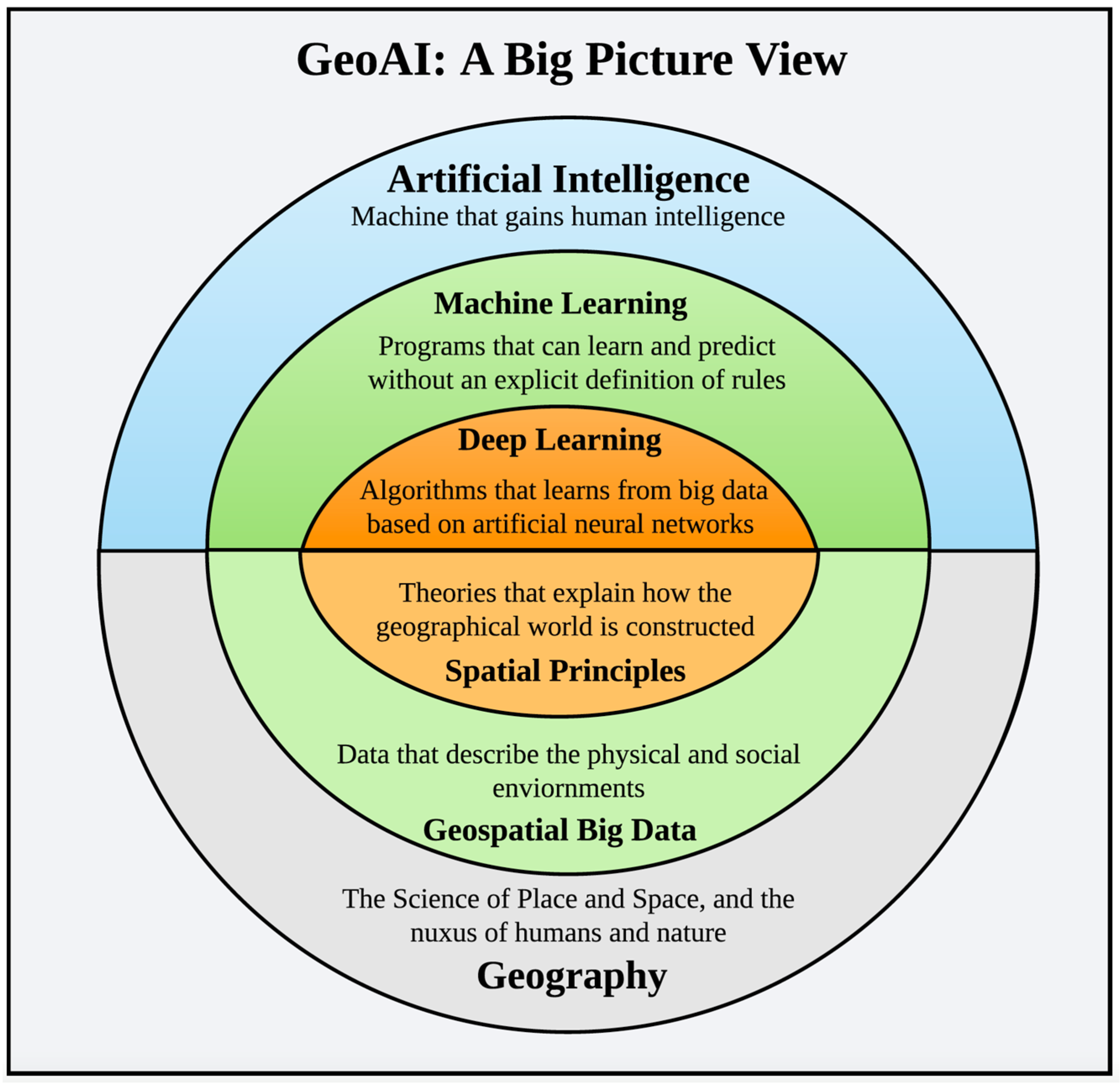
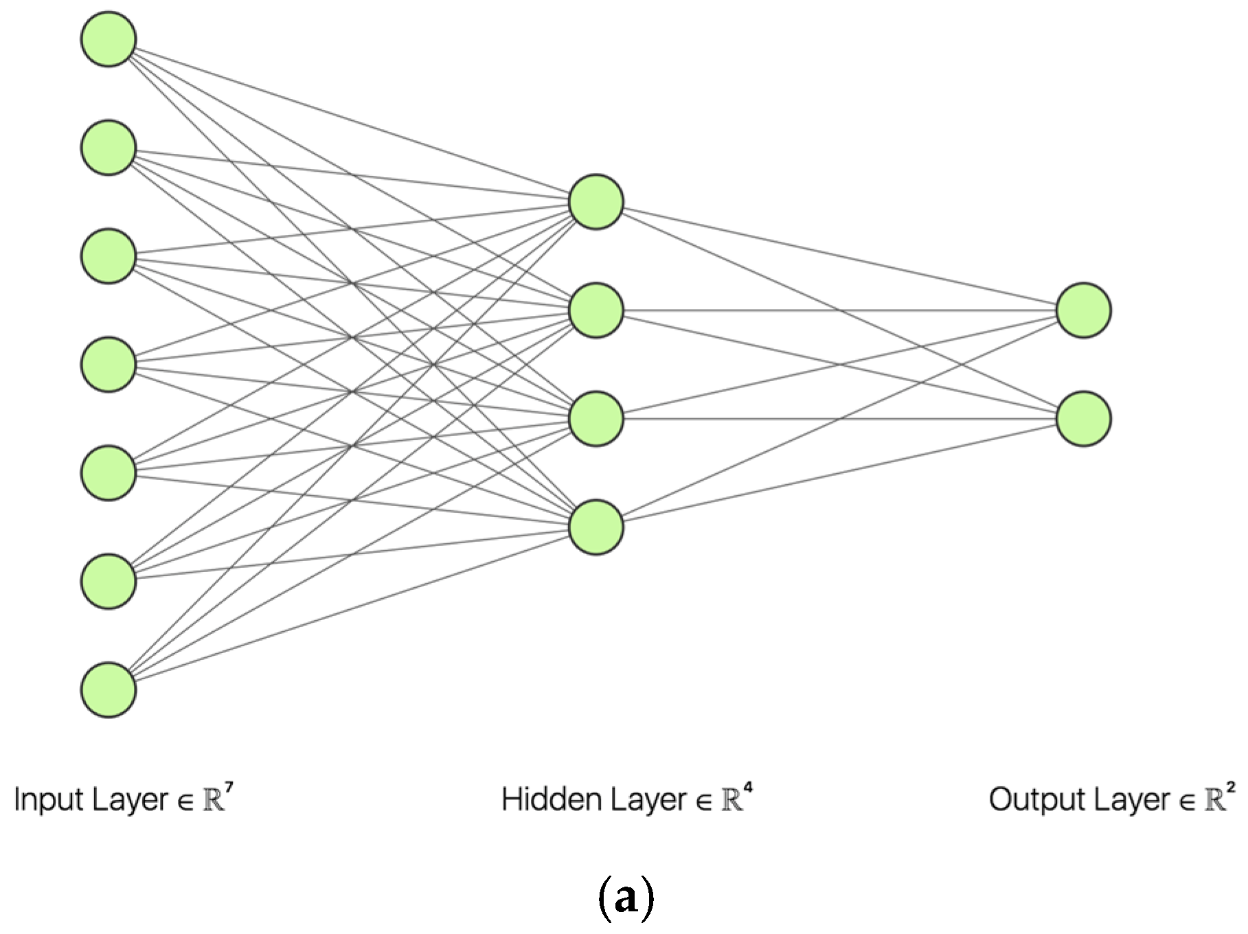
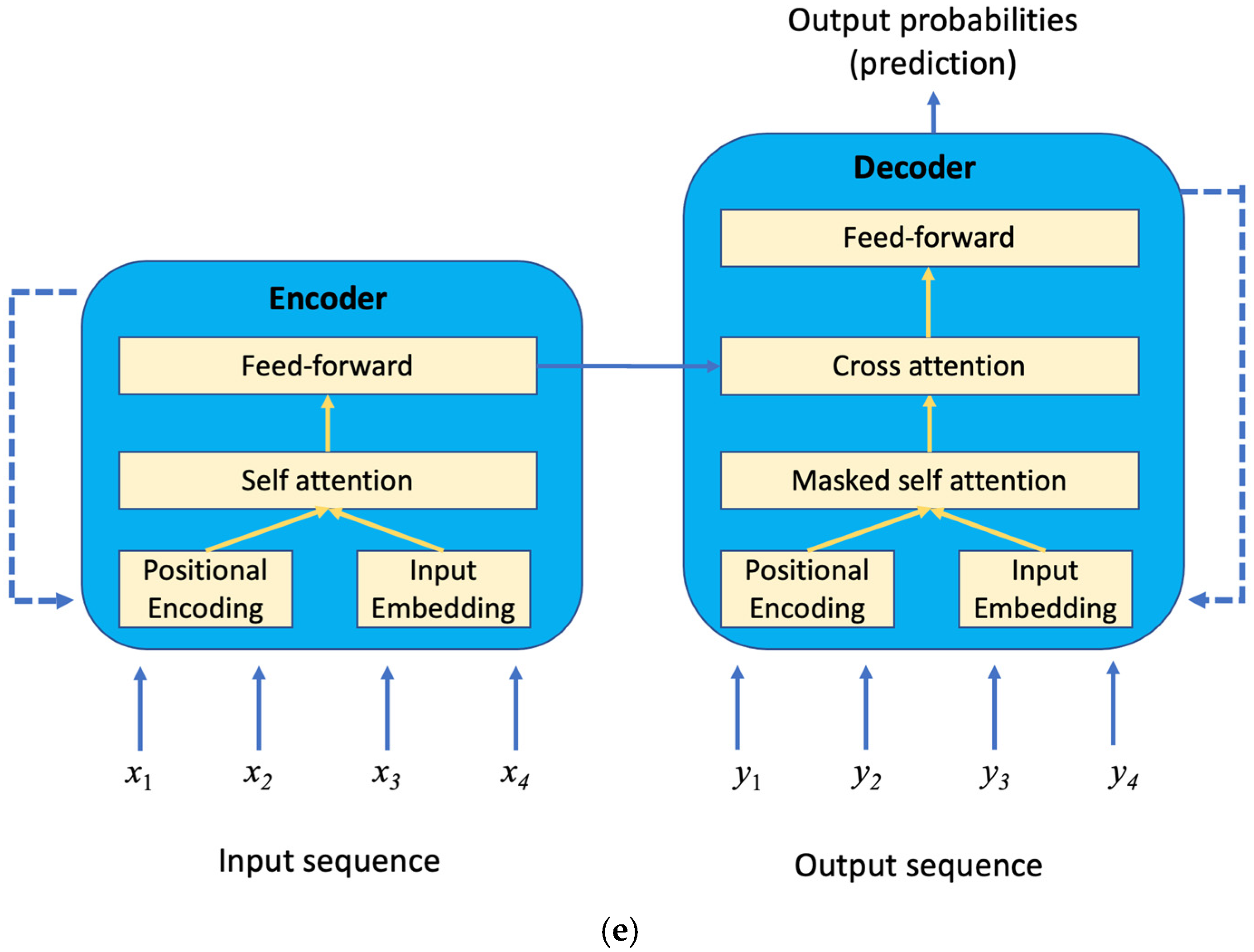
Table 1.
Summary of GeoAI and deep learning applications in remote sensing image analysis.
| Task | Applications | Conventional Approaches | Limitations of Conventional Approaches | Deep Learning (DL) Approaches |
|---|---|---|---|---|
| Image-level classification | ||||
| Land use/land cover analysis Natural feature classify cation Manmade feature classification | Maximum likelihood Minimum distance Support vector machine (SVM) Principal component analysis (PCA) | Subjective feature extraction Not suitable for large datasets | Convolutional neural network (CNN) Graph neural network (GNN) Combination of CNN and GNN | |
| Object detection | ||||
| Environmental management Urban planning Search and rescue operations Inspection of living conditions of underserved communities | Template matching Knowledge-based Object-based Machine learning-based | Sensitive to shape and density change Subjective prior knowledge and detection rules Lack of full automation process | Region-based CNN Regression-based CNN | |
| Semantic segmentation | ||||
| Precision agriculture Land use/land cover analysis Infrastructure (road) extraction | Region-based Edge-based Clustering-based | Sensitive to contrast between objects and the background Subjective parameter selection | Encoder/decoder-based CNN | |
| Height/depth estimation | ||||
| 3D modeling Smart cities Ocean engineering | LiDAR and digital service model (DSM) Monocular estimation Stereo matching | Hand-crafted features Need for careful camera alignment | CNN-based monocular estimation CNN-based stereo matching | |
| Image super resolution | ||||
| Image quality improvement in applications like medical imaging and remote sensing | Interpolation Statistical models Probability models | Subjective parameter selection Ill-posed problem, requirement of prior information | CNN-based methods GAN-based methods | |
| Object tracking | ||||
| Vehicle tracking Automated surveillance Video indexing Human-computer interaction | Object detection, object feature selection and motion modeling | Hand-crafted features Subjective prior knowledge and detection rules | CNN-based single object tracking CNN-based multiple object tracking | |
| Change detection | ||||
| Land use/land cover analysis Deformation assessment Damage estimation | Image differencing Image rationing PCA Change vector analysis | Subjective parameter selection (change threshold) Unable to extract detailed change information | Object detection-based approaches Segmentation-based approaches | |
| Forecasting | ||||
| Weather forecasting Drought forecasting Land use/land cover forecasting Sales forecasting | Moving averages Exponential smoothing Linear regressions Probability models | Suitable for short-term/univariate forecasting Lag forecasts behind the actual trend | Deep Belief Network Long Short-Term Memory (LSTM) Transformer | |
Table 2.
Summary of GeoAI and deep learning applications in street view image analysis.
| Task | Applications | Conventional Approaches | Limitations of Conventional Approaches | Machine Learning (ML)/DL Approaches |
|---|---|---|---|---|
| Quantification of neighborhood properties | ||||
| Infer social and environmental properties of an urban region | In-person interviews | Labor-intensive Lack of data | Classification Object detection | |
| Calculation of sky view factors | ||||
| Urban management Geomorphology Climate modeling | Direct measurement Simulation | On-site work required Hard to get precise parameters in complex scenes | Semantic segmentation | |
| Neighborhood change monitoring | ||||
| Urban management Policies evaluation | In-person interviews Mailed questionnaires Visual perception surveys | Human bias Small region coverage | Semantic segmentation Classification | |
| Identification of human perception of places | ||||
| Geospatial intelligence Cognitive and behavioral science | Indirect and direct human communication | Human bias Small region coverage | Object detection (face) Classification (emotion) | |
| Personality and place uniqueness mining | ||||
| Human activity Socioeconomic factors | In-person interviews Social surveys | Human bias Small region coverage | Classification Object detection Semantic segmentation | |
| Human activity prediction | ||||
| Urban planning Policies evaluation Assessment of health and environmental impacts | Household surveys In-person interviews Questionnaires | Labor-intensive Resource-intensive Lag of data | Object detection Classification | |
Table 3.
Summary of GeoAI and deep learning applications in geoscientific data analysis, as well as limitations of conventional techniques.
Table 3.
Summary of GeoAI and deep learning applications in geoscientific data analysis, as well as limitations of conventional techniques.
| Task | Applications | Conventional Approaches | Limitation of Conventional Approaches | ML/DL Approaches |
|---|---|---|---|---|
| Precipitation nowcasting | ||||
| Safety guidance for traffic Emergency alerts for hazardous events | NWP-based method Optical flow techniques on radar echo map | Resource-intensive Subjective pre-defined parameters Lack of end-to-end optimization | 2D/3D CNN RNN CNN (spatial correlation) + RNN (temporal dynamics) | |
| Extreme climate events detection | ||||
| Disaster preparation and response | Simulation tools | Subjective pre-defined parameters Inconsistent assessments on the same events | CNN classification on multiple stacked spatial variables 3D CNN | |
| Earthquake detection and phase picking | ||||
| Disaster alerts and response | Picking-based Waveform-based | Weak signal filtering capability Prior information requirement Less sensitive to smaller events | CNN classification on waveform signals RNN for waveform matching CNN (noise filter) + RNN (phase picking) CNN + RNN + transformer | |
| Wildfire spread modeling | ||||
| Safety guidance for firefighters Public risk reducing Urban planning | Physics-based models Cell-based methods Vector-based methods | Subjective assumptions Limited model complexity | 2D/3D CNN | |
| Mesoscale ocean eddy identification and tracking | ||||
| Near-surface winds, clouds, rainfall, and marine ecosystems Ocean energy and nutrient transfer | Physical parameter-based Geometric based | Subjective pre-defined parameters Limited generalization Unclear geometrical features | Classification Object detection Semantic segmentation | |
Publisher’s Note: MDPI stays neutral with regard to jurisdictional claims in published maps and institutional affiliations. |
© 2022 by the authors. Licensee MDPI, Basel, Switzerland. This article is an open access article distributed under the terms and conditions of the Creative Commons Attribution (CC BY) license (https://creativecommons.org/licenses/by/4.0/).
Share and Cite
MDPI and ACS Style
Li, W.; Hsu, C.-Y. GeoAI for Large-Scale Image Analysis and Machine Vision: Recent Progress of Artificial Intelligence in Geography. ISPRS Int. J. Geo-Inf. 2022, 11, 385. https://doi.org/10.3390/ijgi11070385
AMA Style
Li W, Hsu C-Y. GeoAI for Large-Scale Image Analysis and Machine Vision: Recent Progress of Artificial Intelligence in Geography. ISPRS International Journal of Geo-Information. 2022; 11(7):385. https://doi.org/10.3390/ijgi11070385
Chicago/Turabian StyleLi, Wenwen, and Chia-Yu Hsu. 2022. "GeoAI for Large-Scale Image Analysis and Machine Vision: Recent Progress of Artificial Intelligence in Geography" ISPRS International Journal of Geo-Information 11, no. 7: 385. https://doi.org/10.3390/ijgi11070385
Note that from the first issue of 2016, this journal uses article numbers instead of page numbers. See further details here.