

Exploring the Applicability of Self-Organizing Maps for Ecosystem Service Zoning of the Guangdong-Hong Kong-Macao Greater Bay Area
 , , , , and
Abstract
:1. Introduction
2. Spatial Zoning for Facilitating Sustainable Ecosystem Services
3. Materials and Methods
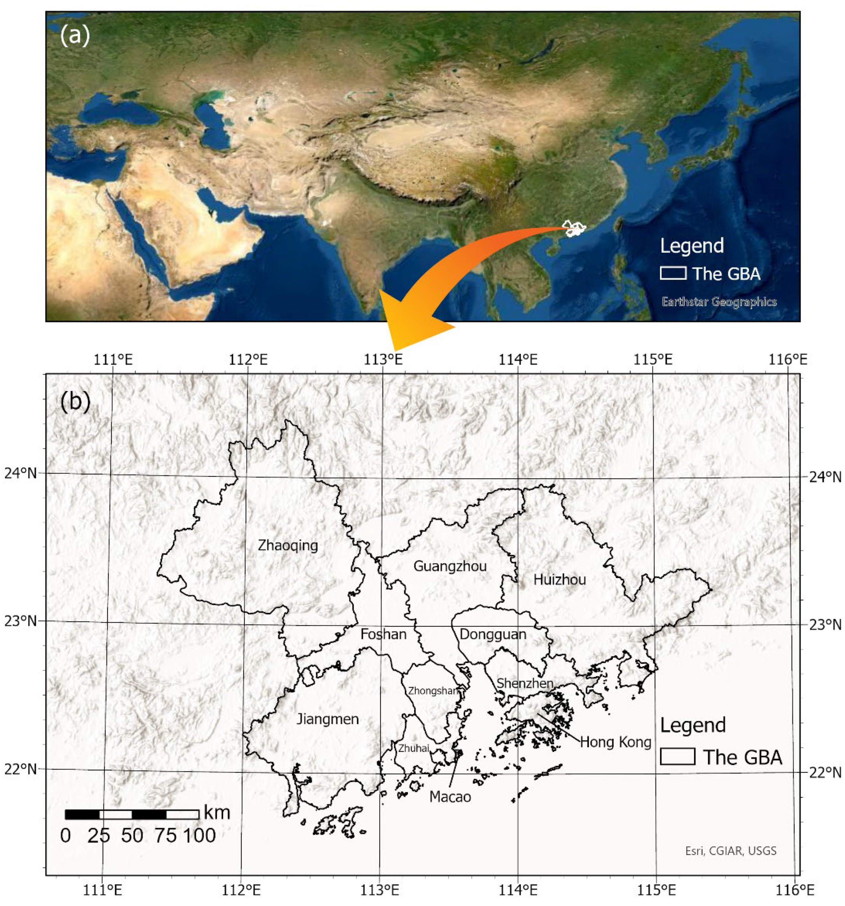
3.1. Study Area
3.2. Ecosystem Services
3.3. ESV Zoning
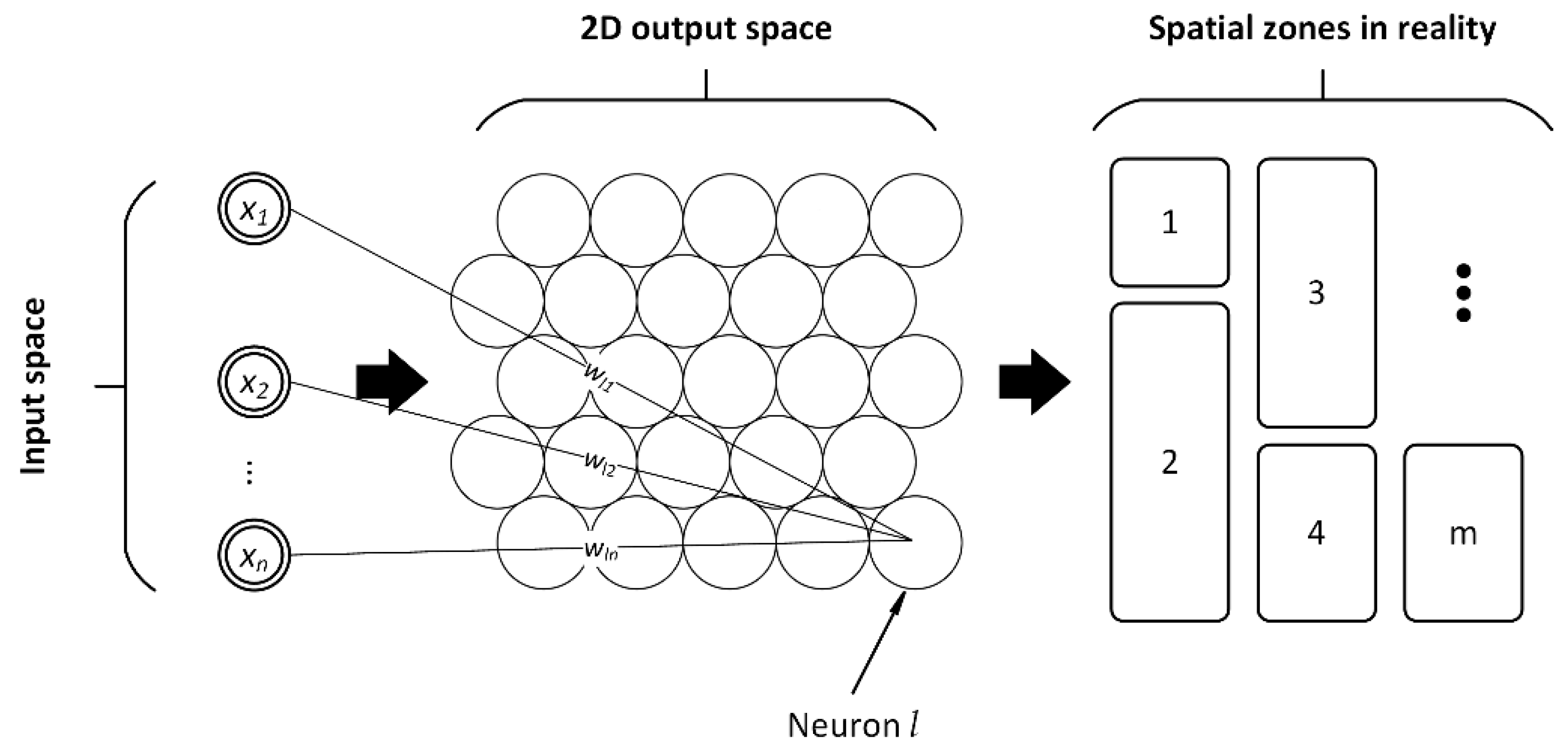
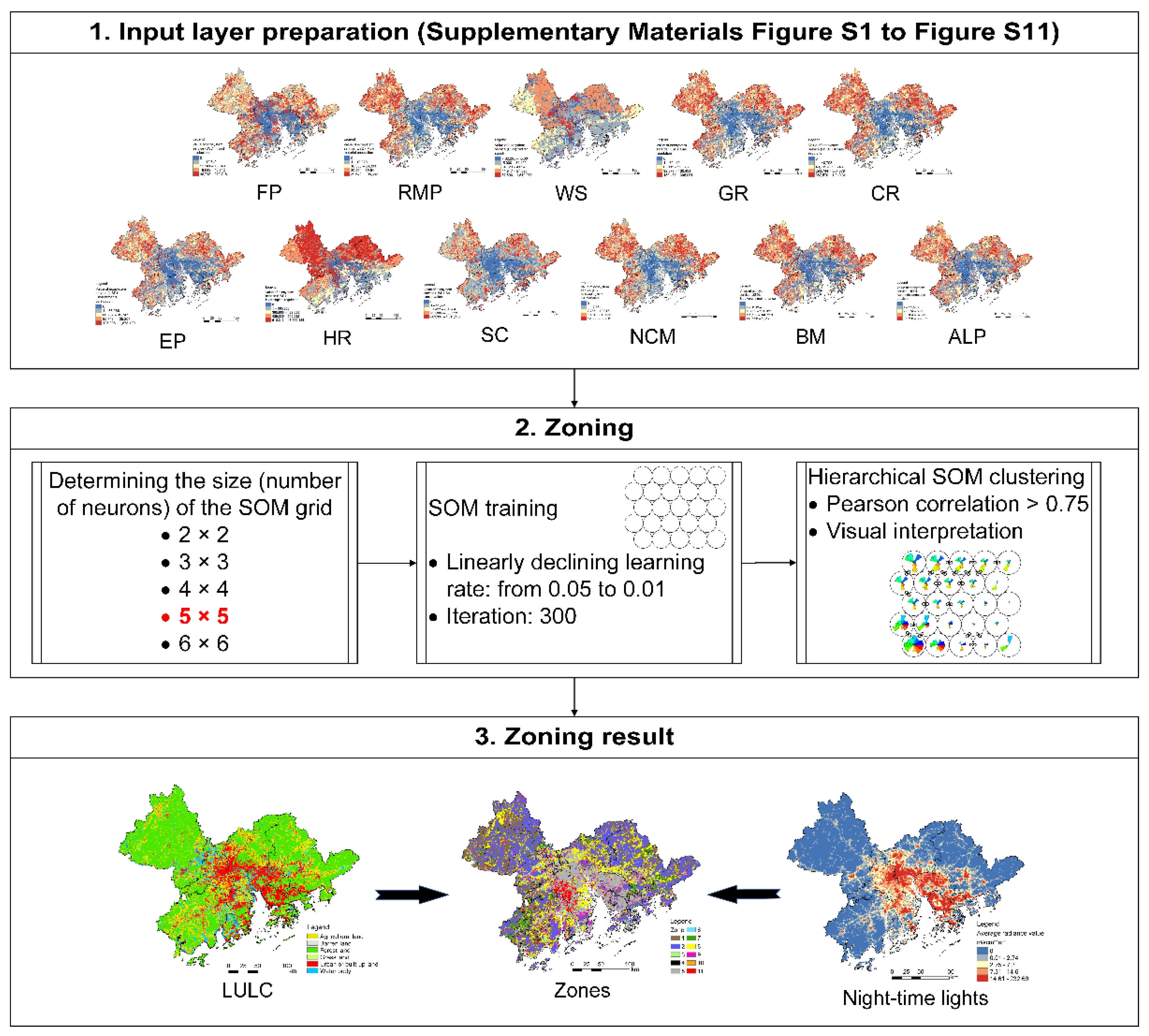
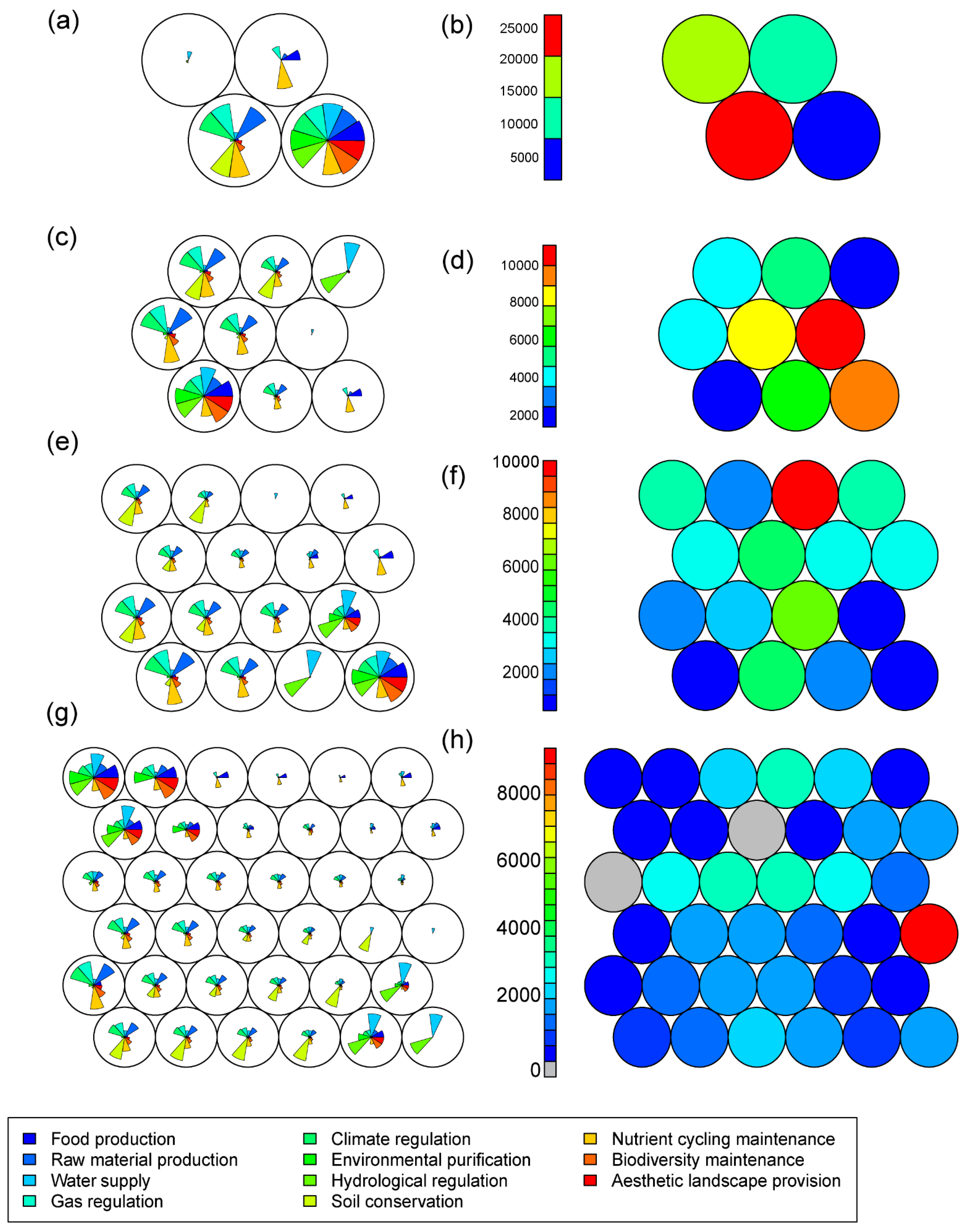
3.3.1. SOM Zoning
3.3.2. Zonal Characteristic Analysis
4. Results
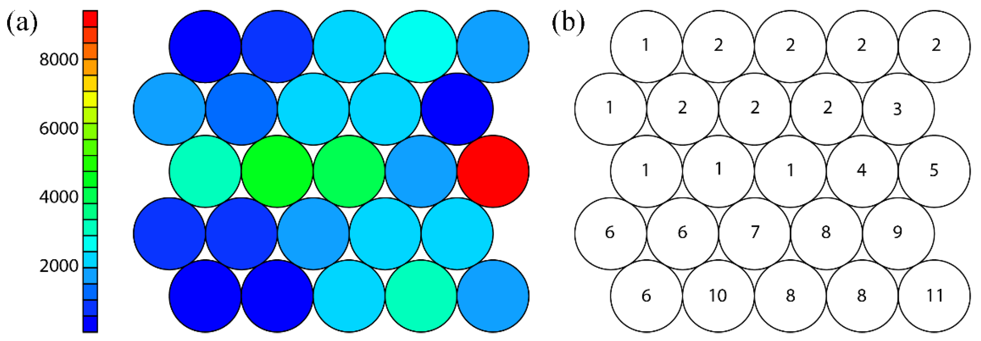
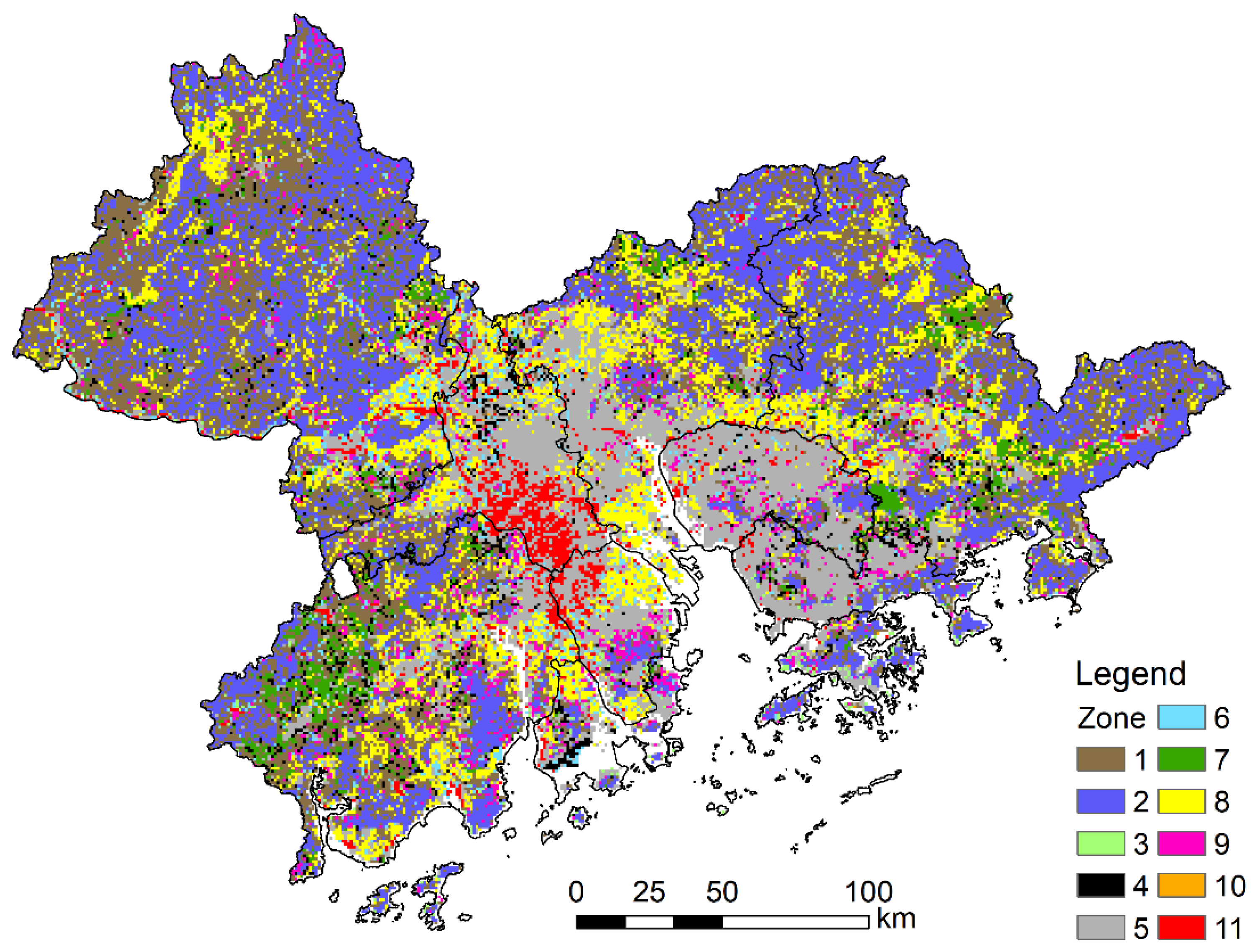
4.1. Ecosystem Service Zones and Their Characteristics
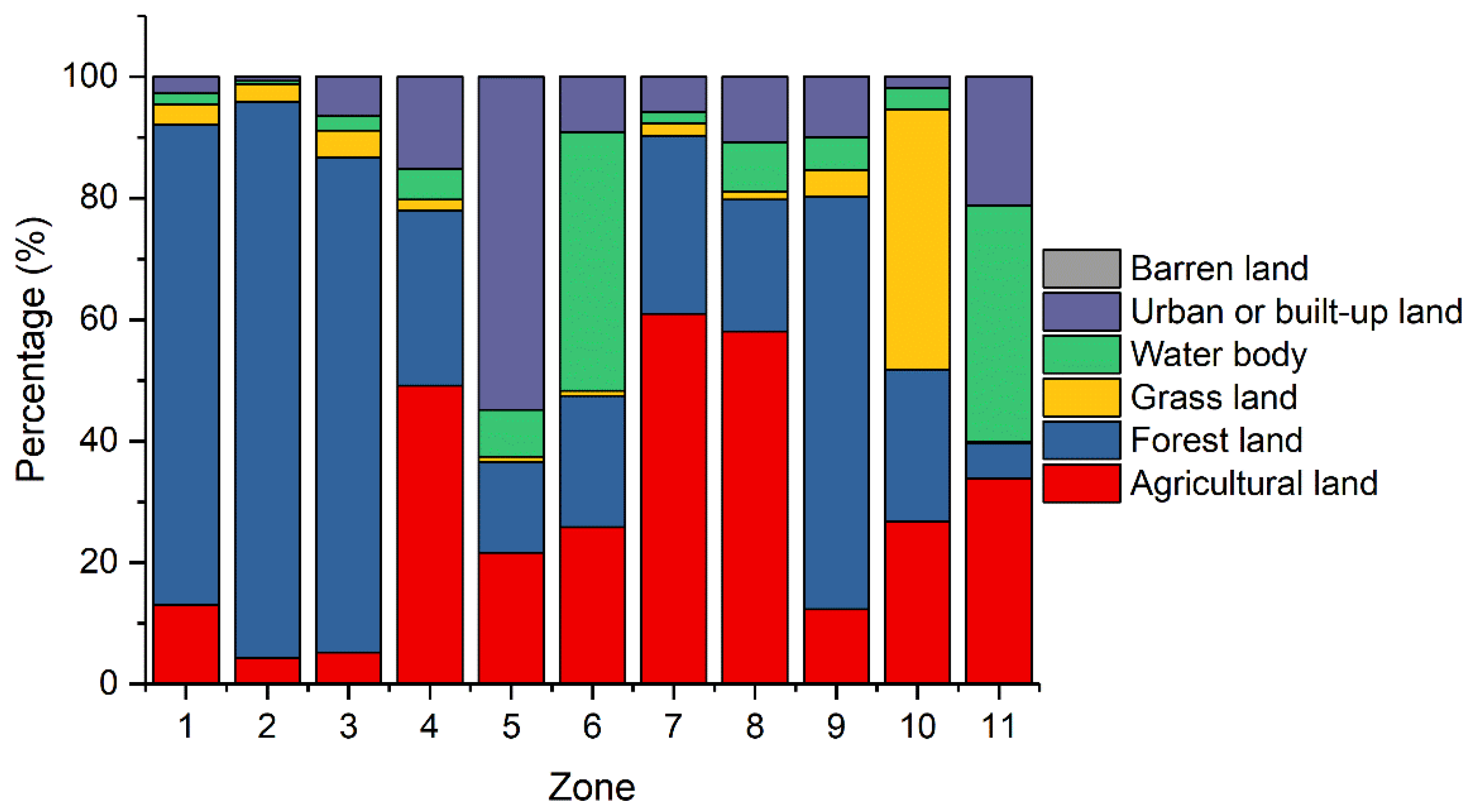
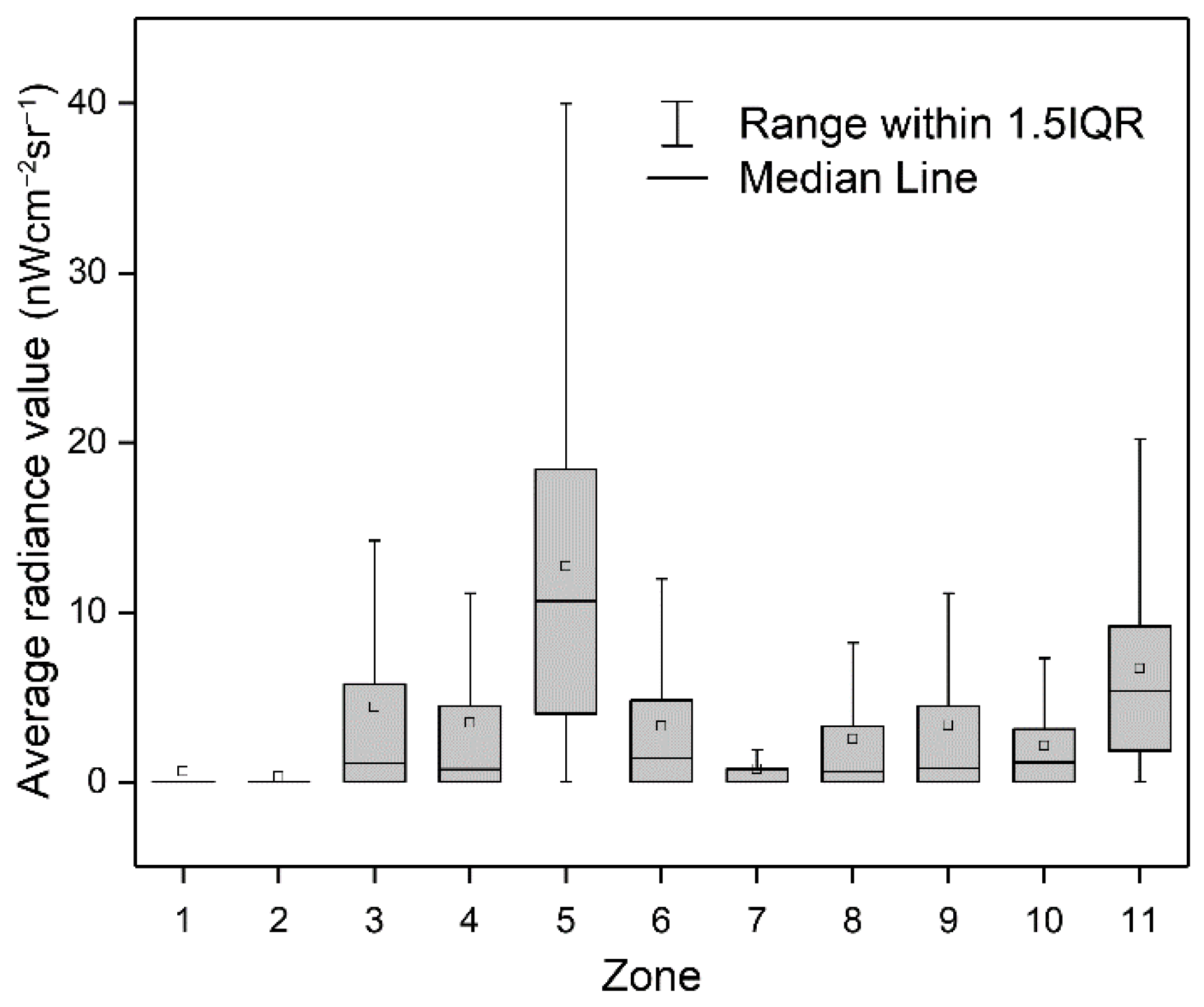
4.2. Zonal Characteristics Based on External Variables
5. Discussion
5.1. Use of the ESV Zoning Map
5.2. Recommendations
6. Conclusions
Supplementary Materials
Author Contributions
Funding
Institutional Review Board Statement
Informed Consent Statement
Data Availability Statement
Acknowledgments
Conflicts of Interest
Abbreviations
| Acronym | Full spelling |
| GBA | Guangdong-Hong Kong-Macao Greater Bay Area |
| ESV | ecosystem service values |
| SOM | self-organizing maps |
| FP | Food production |
| RMP | Raw material production |
| WS | Water supply |
| GR | Gas regulation |
| CR | Climate regulation |
| EP | Environmental purification |
| HR | Hydrological regulation |
| SC | Soil conservation |
| NCM | Nutrient cycling maintenance |
| BM | Biodiversity maintenance |
| ALP | Aesthetic landscape provision |
| GDP | Gross Domestic Product |
| USD | United States dollar |
| RMB | Renminbi |
| HKD | Hong Kong dollar |
| MOP | Macanese pataca |
| LULC | land use/land cover |
| BMU | best matching unit |
| VIIRS | Visible Infrared Imaging Radiometer Suite |
References
- Ma, P.; Wang, W.; Zhang, B.; Wang, J.; Shi, G.; Huang, G.; Chen, F.; Jiang, L.; Lin, H. Remotely sensing large- and small-scale ground subsidence: A case study of the Guangdong–Hong Kong–Macao greater bay area of China. Remote Sens. Environ. 2019, 232, 111282. [Google Scholar] [CrossRef]
- Hui, E.C.M.; Li, X.; Chen, T.; Lang, W. Deciphering the spatial structure of China’s megacity region: A new bay area—The Guangdong-Hong Kong-Macao greater bay area in the making. Cities 2018, 105, 102168. [Google Scholar] [CrossRef]
- Govada, S.S.; Rodgers, T. Towards smarter regional development of hong kong within the greater bay area. In Smart Metropolitan Regional Development: Economic and Spatial Design Strategies; Kumar, T.M.V., Kozhikode, K., Eds.; Springer Nature Singapore Pte Ltd.: Singapore, 2019; pp. 101–171. [Google Scholar]
- Chen, Z.; Li, Y.; Wang, P. Transportation accessibility and regional growth in the greater bay area of China. Transp. Res. Part D Transp. Environ. 2020, 86, 102453. [Google Scholar] [CrossRef]
- Yang, C.; Li, Q.; Hu, Z.; Chen, J.; Shi, T.; Ding, K.; Wu, G. Spatiotemporal evolution of urban agglomerations in four major bay areas of US, China and Japan from 1987 to 2017: Evidence from remote sensing images. Sci. Total Environ. 2019, 671, 232–247. [Google Scholar] [CrossRef]
- Li, L.C.; Kwok, M.-T. Unpacking the plan for the Guangdong–Hong Kong–Macao greater bay area: A mechanism for reform. China World 2019, 2, 1950010. [Google Scholar] [CrossRef]
- Li, H.; Jin, R.; Ning, X.; Skitmore, M.; Zhang, T. Prioritizing the sustainability objectives of major public projects in the Guangdong–Hong Kong–Macao greater bay area. Sustainability 2018, 10, 4110. [Google Scholar] [CrossRef]
- Fang, X.; Fan, Q.; Liao, Z.; Xie, J.; Xu, X.; Fan, S. Spatial-temporal characteristics of the air quality in the Guangdong−Hong Kong−Macau greater bay area of China during 2015–2017. Atmos. Environ. 2019, 210, 14–34. [Google Scholar] [CrossRef]
- Gan, L.; Chen, Y.; Wu, Z.; Qian, Q.; Zheng, Z. The variation of ecological sensitivity in guangdong hong kong macao greater bay area in recent 20 years. Chin. J. Ecol. 2018, 8, 2453–2462. (In Chinese) [Google Scholar]
- Bi, M.; Xie, G.; Yao, C. Ecological security assessment based on the renewable ecological footprint in the guangdong-hong kong-macao greater bay area, china. Ecol. Indic. 2020, 116, 106432. [Google Scholar] [CrossRef]
- Costanza, R.; de Groot, R.; Sutton, P.; van der Ploeg, S.; Anderson, S.J.; Kubiszewski, I.; Farber, S.; Turner, R.K. Changes in the global value of ecosystem services. Glob. Environ. Chang. 2014, 26, 152–158. [Google Scholar] [CrossRef]
- Han, R.; Feng, C.-C.; Xu, N.; Guo, L. Spatial heterogeneous relationship between ecosystem services and human disturbances: A case study in Chuandong, China. Sci. Total Environ. 2020, 721, 137818. [Google Scholar] [CrossRef]
- Su, S.; Li, D.; Hu, Y.n.; Xiao, R.; Zhang, Y. Spatially non-stationary response of ecosystem service value changes to urbanization in Shanghai, China. Ecol. Indic. 2014, 45, 332–339. [Google Scholar] [CrossRef]
- Keeney, R.L. Value-focused thinking: Identifying decision opportunities and creating alternatives. Eur. J. Oper. Res. 1996, 92, 537–549. [Google Scholar] [CrossRef]
- Valuation of Ecosystem Services. Available online: http://www.ecosystemvaluation.org/1-02.htm (accessed on 13 March 2020).
- Kubiszewski, I.; Costanza, R.; Anderson, S.; Sutton, P. The future value of ecosystem services: Global scenarios and national implications. Ecosyst. Serv. 2017, 26, 289–301. [Google Scholar] [CrossRef]
- Chen, Z.; Zhang, X. Value of ecosystem services in China. Chin. Sci. Bull. 2000, 45, 870–876. [Google Scholar] [CrossRef]
- Xie, G.; Zhang, C.; Zhang, C.; Xiao, Y.; Lu, C. The value of ecosystem services in China. Resour. Sci. 2015, 37, 1740–1746. (In Chinese) [Google Scholar]
- Wang, X.; Yan, F.; Su, F. Impacts of urbanization on the ecosystem services in the Guangdong-Hong Kong-Macao greater bay area, China. Remote Sens. 2020, 12, 3269. [Google Scholar] [CrossRef]
- Zhang, C.; Zhao, Q.; Tang, H.; Qian, W.; Su, M.; Pan, L. How well do three tree species adapt to the urban environment in Guangdong-Hong Kong-Macao greater bay area of China regarding their growth patterns and ecosystem services? Forests 2020, 11, 420. [Google Scholar] [CrossRef]
- Valenti, W.C.; Kimpara, J.M.; Preto, B.d.L.; Moraes-Valenti, P. Indicators of sustainability to assess aquaculture systems. Ecol. Indic. 2018, 88, 402–413. [Google Scholar] [CrossRef]
- Waas, T.; Hugé, J.; Block, T.; Wright, T.; Benitez-Capistros, F.; Verbruggen, A. Sustainability assessment and indicators: Tools in a decision-making strategy for sustainable development. Sustainability 2014, 6, 5512–5534. [Google Scholar] [CrossRef]
- Kohonen, T. Self-organized formation of topologically correct feature maps. Biol. Cybern. 1982, 43, 59–69. [Google Scholar] [CrossRef]
- Kohonen, T. The self-organizing map. Proc. IEEE 1990, 78, 1464–1480. [Google Scholar] [CrossRef]
- Wang, L.; Li, Z.; Wang, D.; Hu, X.; Ning, K. Self-organizing map network-based soil and water conservation partitioning for small watersheds: Case study conducted in Xiaoyang watershed, China. Sustainability 2020, 12, 2126. [Google Scholar] [CrossRef]
- Steiger, E.; Resch, B.; Zipf, A. Exploration of spatiotemporal and semantic clusters of twitter data using unsupervised neural networks. Int. J. Geogr. Inf. Sci. 2016, 30, 1694–1716. [Google Scholar] [CrossRef]
- Steiger, E.; Resch, B.; de Albuquerque, J.P.; Zipf, A. Mining and correlating traffic events from human sensor observations with official transport data using self-organizing-maps. Transp. Res. Part C Emerg. Technol. 2016, 73, 91–104. [Google Scholar] [CrossRef]
- Nikoo, M.R.; Mahjouri, N. Water quality zoning using probabilistic support vector machines and self-organizing maps. Water Resour. Manag. 2013, 27, 2577–2594. [Google Scholar] [CrossRef]
- Fei, D.; Cheng, Q.; Mao, X.; Liu, F.; Zhou, Q. Land use zoning using a coupled gridding-self-organizing feature maps method: A case study in China. J. Clean. Prod. 2017, 161, 1162–1170. [Google Scholar] [CrossRef]
- Tsuchiya, T. Kansei engineering study for streetscape zoning using self organizing maps. Int. J. Affect. Eng. 2013, 12, 365–373. [Google Scholar] [CrossRef]
- Zamani, A.; Nedaei, M. Application of som neural network for numerical tectonic zoning: A new approach for tectonic zoning of Iran. Geosciences 2010, 19, 83–88. [Google Scholar]
- Huang, F.; Yin, K.; Huang, J.; Gui, L.; Wang, P. Landslide susceptibility mapping based on self-organizing-map network and extreme learning machine. Eng. Geol. 2017, 223, 11–22. [Google Scholar] [CrossRef]
- Bennett, E.M.; Chaplin-Kramer, R. Science for the sustainable use of ecosystem services. F1000Research 2016, 5, 2622. [Google Scholar] [CrossRef]
- Dearing, J.A.; Yang, X.; Dong, X.; Zhang, E.; Chen, X.; Langdon, P.G.; Zhang, K.; Zhang, W.; Dawson, T.P. Extending the timescale and range of ecosystem services through paleoenvironmental analyses, exemplified in the lower Yangtze basin. Proc. Natl. Acad. Sci. USA 2012, 109, E1111–E1120. [Google Scholar] [CrossRef]
- Tomscha, S.A.; Sutherland, I.J.; Renard, D.; Gergel, S.E.; Rhemtulla, J.M.; Bennett, E.M.; Daniels, L.D.; Eddy, I.M.S.; Clark, E.E. A guide to historical data sets for reconstructing ecosystem service change over time. BioScience 2016, 66, 747–762. [Google Scholar] [CrossRef] [Green Version]
- Renard, D.; Rhemtulla, J.M.; Bennett, E.M. Historical dynamics in ecosystem service bundles. Proc. Natl. Acad. Sci. USA 2015, 112, 13411–13416. [Google Scholar] [CrossRef]
- Foster, D.; Swanson, F.; Aber, J.; Burke, I.; Brokaw, N.; Tilman, D.; Knapp, A. The importance of land-use legacies to ecology and conservation. BioScience 2003, 53, 77–88. [Google Scholar] [CrossRef]
- Liu, J.; Yang, W.; Li, S. Framing ecosystem services in the telecoupled anthropocene. Front. Ecol. Environ. 2016, 14, 27–36. [Google Scholar] [CrossRef]
- Chan, K.M.A.; Shaw, M.R.; Cameron, D.R.; Underwood, E.C.; Daily, G.C. Conservation planning for ecosystem services. PLoS Biol. 2006, 4, e379. [Google Scholar] [CrossRef]
- Xu, Z.; Peng, J.; Dong, J.; Liu, Y.; Liu, Q.; Lyu, D.; Qiao, R.; Zhang, Z. Spatial correlation between the changes of ecosystem service supply and demand: An ecological zoning approach. Landsc. Urban Plan. 2022, 217, 104258. [Google Scholar] [CrossRef]
- Abdollahi, A.A.; Babazadeh, H.; Yargholi, B.; Taghavi, L. Zoning the rate of pollution in domestic river using spatial multi-criteria evaluation model. Civ. Environ. Eng. 2020, 16, 49–62. [Google Scholar] [CrossRef]
- Yang, L.; Lyu, K.; Li, H.; Liu, Y. Building climate zoning in china using supervised classification-based machine learning. Build. Environ. 2020, 171, 106663. [Google Scholar] [CrossRef]
- Liu, Y.; Li, T.; Zhao, W.; Wang, S.; Fu, B. Landscape functional zoning at a county level based on ecosystem services bundle: Methods comparison and management indication. J. Environ. Manag. 2019, 249, 109315. [Google Scholar] [CrossRef]
- Pérez-Hoyos, A.; Martínez, B.; García-Haro, F.J.; Moreno, Á.; Gilabert, M.A. Identification of ecosystem functional types from coarse resolution imagery using a self-organizing map approach: A case study for Spain. Remote Sens. 2014, 6, 11391–11419. [Google Scholar] [CrossRef]
- The Resource and Environment Data Center. Available online: https://www.resdc.cn/ (accessed on 22 August 2022).
- Xu, X. (Ed.) Dataset of the Spatial Distribution of the Value of Ecosystem Services in China; The Resource and Environment Data Cloud Platform of the Chinese Academy of Sciences: Beijing, China, 2018. [Google Scholar]
- Guangdong Statistical Yearbook. Available online: http://stats.gd.gov.cn/gdtjnj/ (accessed on 22 August 2022).
- The World Bank Open Data. Available online: https://data.worldbank.org/ (accessed on 22 August 2022).
- Census and Statistics Department of Hong Kong. Available online: https://www.censtatd.gov.hk/home/ (accessed on 24 August 2022).
- Worldometer. Available online: https://www.worldometers.info/ (accessed on 22 August 2022).
- Geographical Information Monitoring Cloud Platform. Available online: http://www.dsac.cn/ (accessed on 22 August 2022).
- Wehrens, R.; Buydens, L.M. Self-and super-organizing maps in r: The kohonen package. J. Stat. Softw. 2007, 21, 1–19. [Google Scholar] [CrossRef] [Green Version]
- Augustijn, E.W.; Zurita-Milla, R. Self-organizing maps as an approach to exploring spatiotemporal diffusion patterns. Int. J. Health Geogr. 2013, 12, 60. [Google Scholar] [CrossRef]
- Yan, Y.; Wang, Y.-C.; Feng, C.-C.; Wan, P.-H.M.; Chang, K.T.-T. Potential distributional changes of invasive crop pest species associated with global climate change. Appl. Geogr. 2017, 82, 83–92. [Google Scholar] [CrossRef]
- Huang, Q.; Yang, X.; Gao, B.; Yang, Y.; Zhao, Y. Application of dmsp/ols nighttime light images: A meta-analysis and a systematic literature review. Remote Sens. 2014, 6, 6844–6866. [Google Scholar] [CrossRef]
- National Oceanic and Atmospheric Administration of the United States of America. Available online: https://ngdc.noaa.gov/eog/viirs/download_dnb_composites.html (accessed on 22 August 2022).
- Burkhard, B.; Maes, J. Mapping Ecosystem Services; Pensoft Publishers: Sofia, Bulgaria, 2017. [Google Scholar]
- UN. Agenda 21 of the United Nations Conference on Environment & Development; United Nations Publications: Rio de Janerio, Brazil, 1992. [Google Scholar]
- Outline Development Plan for the Guangdong-Hong Hong-Macao Greater Bay Area. Available online: http://www.gov.cn/zhengce/2019-02/18/content_5366593.htm#1 (accessed on 22 August 2022).
- Vollmer, D.; Pribadi, D.O.; Remondi, F.; Rustiadi, E.; Grêt-Regamey, A. Prioritizing ecosystem services in rapidly urbanizing river basins: A spatial multi-criteria analytic approach. Sustain. Cities Soc. 2016, 20, 237–252. [Google Scholar] [CrossRef]
- Yang, W.; Dietz, T.; Kramer, D.B.; Ouyang, Z.; Liu, J. An integrated approach to understanding the linkages between ecosystem services and human well-being. Ecosyst. Health Sustain. 2015, 1, 1–12. [Google Scholar] [CrossRef]
- Yang, W.; Dietz, T.; Liu, W.; Luo, J.; Liu, J. Going beyond the millennium ecosystem assessment: An index system of human dependence on ecosystem services. PLoS ONE 2013, 8, e64581. [Google Scholar] [CrossRef] [PubMed]
- Reyers, B.; Biggs, R.; Cumming, G.S.; Elmqvist, T.; Hejnowicz, A.P.; Polasky, S. Getting the measure of ecosystem services: A social–ecological approach. Front. Ecol. Environ. 2013, 11, 268–273. [Google Scholar] [CrossRef]
- Martín-López, B.; Iniesta-Arandia, I.; García-Llorente, M.; Palomo, I.; Casado-Arzuaga, I.; Amo, D.G.D.; Gómez-Baggethun, E.; Oteros-Rozas, E.; Palacios-Agundez, I.; Willaarts, B.; et al. Uncovering ecosystem service bundles through social preferences. PLoS ONE 2012, 7, e38970. [Google Scholar] [CrossRef] [Green Version]


| Level 1 | Level 2 |
|---|---|
| Provisioning service | Food production (FP) |
| Raw material production (RMP) | |
| Water supply (WS) | |
| Regulating service | Gas regulation (GR) |
| Climate regulation (CR) | |
| Environmental purification (EP) | |
| Hydrological regulation (HR) | |
| Supporting service | Soil conservation (SC) |
| Nutrient cycling maintenance (NCM) | |
| Biodiversity maintenance (BM) | |
| Cultural service | Aesthetic landscape provision (ALP) |
| City | Overall ESV (Billion USD) | 2018 GDP (Billion USD) | 2018 Population (Million) | Overall ESV per Capita (USD/Person) | 2018 GDP per Capita (USD/Person) |
|---|---|---|---|---|---|
| Zhaoqing | 31.47 | 31.43 | 4.15 | 7580 | 7570 |
| Huizhou | 20.38 | 58.57 | 4.83 | 4219 | 12,126 |
| Jiangmen | 17.04 | 41.4 | 4.6 | 3706 | 9004 |
| Foshan | 16.67 | 141.83 | 7.91 | 2109 | 17,940 |
| Guangzhou | 12.45 | 326.3 | 14.9 | 835 | 21,893 |
| Zhongshan | 4.48 | 51.85 | 3.31 | 1352 | 15,666 |
| Dongguan | 3.56 | 118.17 | 8.39 | 424 | 14,081 |
| Shenzhen | 1.6 | 345.75 | 13.03 | 123 | 26,542 |
| Zhuhai | 1.36 | 41.61 | 1.89 | 717 | 22,001 |
| Hong Kong | 0.92 | 362.68 | 7.49 | 123 | 48,409 |
| Macao | 0.001 | 55.08 | 0.67 | 2 | 82,483 |
| Total | 109.93 | 1574.66 | 71.16 | N.A. | N.A. |
| Mean | 9.99 | 143.15 | 6.47 | 1926 | 25,247 |
| LULC | Overall ESV (Billion USD) | Mean ESV (Million USD/km2) |
|---|---|---|
| Agricultural land | 22.94 | 1.98 |
| Barren land | 0.01 | 1.64 |
| Forest land | 52.50 | 1.82 |
| Grass land | 2.00 | 1.72 |
| Urban or built-up land | 9.86 | 1.31 |
| Water body | 22.03 | 6.84 |
| Zone | Main Ecological Services | Overall ESV (Billion USD) | Mean ESV (Million USD/km2) |
|---|---|---|---|
| 1 | Provisioning service (RMP), regulating service (GR and CR), and supporting service (NCM) | 21.22 | 1.55 |
| 2 | Provisioning service (RMP), regulating service (GR and CR), and supporting service (SC and NCM) | 28.09 | 2.11 |
| 3 | Provisioning service (WS) and supporting service (SC) | 0.50 | 1.30 |
| 4 | Provisioning service (FP, RMP, and WS) and supporting service (NCM) | 0.56 | 0.36 |
| 5 | Provisioning service (WS) | 2.68 | 0.29 |
| 6 | Provisioning service (FP, RMP, and WS), regulating service (GR, CR, EP, and HR), supporting service (NCM and BM), and culture service (ALP) | 27.09 | 17.01 |
| 7 | Provisioning service (FP, RMP, and WS), regulating service (GR), and supporting service (NCM) | 0.67 | 0.39 |
| 8 | Provisioning service (FP), regulating service (GR), and supporting service (NCM) | 2.71 | 0.37 |
| 9 | Provisioning service (RMP and WS), regulating service (GR and CR), and supporting service (NCM) | 2.40 | 1.17 |
| 10 | Provisioning service (FP and RMP), regulating service (GR, CR, and EP), supporting service (NCM and BM), and culture service (ALP) | 0.99 | 17.66 |
| 11 | Provisioning service (WS) and regulating service (HR) | 22.97 | 14.00 |
Publisher’s Note: MDPI stays neutral with regard to jurisdictional claims in published maps and institutional affiliations. |
© 2022 by the authors. Licensee MDPI, Basel, Switzerland. This article is an open access article distributed under the terms and conditions of the Creative Commons Attribution (CC BY) license (https://creativecommons.org/licenses/by/4.0/).
Share and Cite
Yan, Y.; Deng, Y.; Yang, J.; Li, Y.; Ye, X.; Xu, J.; Ye, Y. Exploring the Applicability of Self-Organizing Maps for Ecosystem Service Zoning of the Guangdong-Hong Kong-Macao Greater Bay Area. ISPRS Int. J. Geo-Inf. 2022, 11, 481. https://doi.org/10.3390/ijgi11090481
Yan Y, Deng Y, Yang J, Li Y, Ye X, Xu J, Ye Y. Exploring the Applicability of Self-Organizing Maps for Ecosystem Service Zoning of the Guangdong-Hong Kong-Macao Greater Bay Area. ISPRS International Journal of Geo-Information. 2022; 11(9):481. https://doi.org/10.3390/ijgi11090481
Chicago/Turabian StyleYan, Yingwei, Yingbin Deng, Ji Yang, Yong Li, Xinyue Ye, Jianhui Xu, and Yuyao Ye. 2022. "Exploring the Applicability of Self-Organizing Maps for Ecosystem Service Zoning of the Guangdong-Hong Kong-Macao Greater Bay Area" ISPRS International Journal of Geo-Information 11, no. 9: 481. https://doi.org/10.3390/ijgi11090481