Article

Using Dual Spatial Clustering Models for Urban Fringe Areas Extraction Based on Night-time Light Data: Comparison of NPP/VIIRS, Luojia 1-01, and NASA’s Black Marble

1
College of Civil Engineering, Nanjing Forestry University, Nanjing 210037, China
2
State Key Laboratory of Resources and Environmental Information System, Institute of Geographic Sciences and Natural Resources Research, Chinese Academy of Sciences, Beijing 100101, China
3
Anhui Province Key Laboratory of Physical Geographic Environment, Chuzhou 239004, China
4
Key Laboratory of Virtual Geographic Environment, Ministry of Education, Nanjing Normal University, Nanjing 210023, China
*
Author to whom correspondence should be addressed.
ISPRS Int. J. Geo-Inf. 2023, 12(10), 408; https://doi.org/10.3390/ijgi12100408
Submission received: 7 August 2023 / Revised: 24 September 2023 / Accepted: 28 September 2023 / Published: 4 October 2023

Abstract

:
Night-time light data (NTL) have been extensively utilized to map urban fringe areas, but to date, there has not been a comprehensive evaluation of the existing spatial clustering methods for delineating the urban fringe using different types of night-time light data. Therefore, we first selected three popular sources of night-time light data (i.e., NPP/VIIRS, Luojia 1-01, and NASA’s Black Marble) to identify the urban fringe. The recognition of spatial mutations across the urban–rural gradient was conducted based on changes in night light intensity using a spatial continuous wavelet transform model. Then, we employed three representative dual spatial clustering approaches (i.e., MK-Means, DBSC, and DSC) for extracting urban fringe areas using different NTL. By using dual spatial clustering, the spatial patterns of the mutation points were effectively transformed into homogeneous spatially adjacent clusters, enabling the measurement of similarity between mutation points. Taking Nanjing city, one of China’s megacities, as the study area, we found that (1) Compared with the fragmented and concentrated results obtained from the Luojia 1-01, NASA’s Black Marble and NPP/VIIRS data can effectively capture the abrupt change of urban fringes with NTL variations; (2) DSC provided a reliable approach for accurately extracting urban fringe areas using NASA’s Black Marble data.

1. Introduction

Over the past three decades, the global growth rate of urban land use (80%) has significantly outpaced the population growth rate (52%), leading to substantial development in urban areas [1]. By 2050, it is expected that the ongoing global urbanization process will result in 68% of the global population living in urban areas [2]. Urban fringe areas are located in the transitional zone between urban and rural areas, serving as both the forefront of urban expansion and the most sensitive regions in the process of urbanization. Urban fringe areas, as the outer ring of cities, are influenced by both internal and external human–environment systems and exhibit diverse, interactive, and transitional characteristics [3,4]. However, many problems also arise in urban fringe areas due to the increasing heterogeneity and instability of land use and socioeconomic structure, leading to various urban issues such as resource shortage [5] and environmental contamination [6]. Accurate identification of urban fringe areas is of significant practical importance in controlling urban sprawl, optimizing urban planning, and promoting the rational utilization of land.
NTL can reflect the spatial distribution of population density, economic activity, and urbanization [7]. These kinds of data are accessible in real time and are not restricted by administrative boundaries, overcoming the issue of data discontinuity. The distinct characteristics of NTL enable it not simply to capture the spatial expansion of urbanization but also to reveal the diverse levels of urbanization intensity within urban regions. Therefore, it is well-suited for mapping urban fringe areas [8,9]. Since the 1970s, a series of satellite sensors have been developed to capture night-time light data from space [10], including DMSP-OLS [11], Suomi-NPP VIIRS [12], ISS [13], Luojia-01 [14], Jilin1-03B [15], and SDGSAT-1 [16]. Recent reviews on night lights have primarily concentrated on urban applications utilizing DMSP/OLS and NPP/VIIRS data [17,18]. The DMSP-OLS dataset, despite providing continuous NTL from 1992 to 2013, suffers from limitations such as discontinuity and oversaturation caused by bright lights. To address these limitations, it was replaced by the NPP-VIIRS starting from 2013 [19]. The utilization of NPP-VIIRS data brings substantial improvements to the dataset, including enhanced spatial resolution, reduced saturation issues, and on-board calibration [20]. Recently, researchers have increasingly utilized VIIRS data to extract urban spatial areas at different scales. Since 2018, a series of new VIIRS products with progressively improved image quality have been released. The NASA’s Black Marble product suite (VNP46) is considered the state-of-the-art night-time light data source developed to harness the full potential of the VIIRS time series record [21,22]. The VNP46 product suite offers cloud-free, atmospheric-, terrain-, vegetation-, snow-, lunar-, and stray-light-corrected radiances, enabling researchers to derive valuable insights into urbanization dynamics, environmental changes, and socioeconomic activities [23]. In addition to the aforementioned data, the Luojia 1-01 satellite was successfully launched on 2 June 2018. It boasts a remarkable spatial resolution of 130 m, surpassing the resolutions of NPP/VIIRS at 500 m. This higher spatial resolution enables more detailed and precise observations of night-time light phenomena, greatly enhancing its capabilities for various night-time remote sensing applications. However, even when these data are collected, there has been a lack of comparison to determine how effectively different NTL sources detect urban fringe areas.
Currently, the identification methods of urban fringe areas using NTL mainly consist of threshold analysis, mutation detection, and spatial clustering methods. The threshold analysis method typically employs the night-time light intensity (NLI) index for delineating urban fringes through ratio classification [24,25,26]. While the threshold analysis method is simple and practical, determining the appropriate threshold often requires repeated experiments, which can result in issues such as low efficiency and limited applicability. The mutation detection method calculates the locations of mutation values along the boundaries of the urban fringe and then connects these areas of mutation to map the spatial extent of the urban fringe [27,28]. The mutation detection method is not suitable for identifying arbitrary boundaries, and the boundaries of the urban fringe are intuitively obtained and manually connected. The spatial clustering method first focuses on the recognition of spatial mutations across the urban–rural gradient. Then, classical clustering algorithms are employed to identify a series of spatial clusters, grouping similar pixels within the same fringe cluster [9,29,30]. Compared to the other two methods, the spatial clustering approach is prevalent for urban fringe extraction, utilizing density maps related to urbanization due to its objectivity and convenience [31]. The dual spatial clustering method can take into account both spatial proximity and attribute similarity features, allowing for a better exploration of the distribution patterns and trends of geographic spatial entities [32]. Among them, there are three representative dual spatial approaches, which include MK-Means [33], DBSC [32], and DSC [34]. The MK-Means algorithm is an extension of the K-means algorithm that incorporates attribute metrics to broaden the focus on the spatial object’s attribute distance, aiming to consider both the heterogeneity of spatial positions and the similarity of attributes. Using this approach, Feng [9] discovered more detailed information regarding urban–rural fringes by combining NLI and light fluctuation in comparison to the traditional mutation detection method. The analysis results continue to be challenged by issues such as varying density, arbitrary shapes, and spatial noise problems, which cannot be overlooked. The DBSC algorithm is a clustering method that identifies spatial clusters by modeling the spatial proximity and attribute similarity relationships among spatial objects with the help of constrained Delaunay triangulation. The DBSC algorithm has proven to be efficient and applicable in identifying clusters with irregular shapes and varying densities. It has been successfully used for urban element identification and urban spatial structure analysis [35,36]. However, DBSC algorithm results heavily depend on the global shared non-spatial attribute threshold, failing to capture the inhomogeneous structure of the dataset. DSC can handle both spatial proximity and attribute similarity in the presence of heterogeneity (i.e., the difference of observations in attribute distribution is homogeneous within each cluster but inhomogeneous between clusters) and noise (i.e., attribute values of spatial objects are significantly different from those of other objects in its spatial neighborhood). The detection of these clusters is valuable for gaining insights into the localized patterns of geographical phenomena. Using DSC, Yang [31] can detect the urban–rural fringes with a “Main center–Subcenter” structure using diverse datasets. Nonetheless, the DSC algorithm may result in over-segment clusters when dealing with mixed inhomogeneous and homogeneous dataset structures. These three algorithms differ significantly in terms of theory and accuracy. The lack of a comprehensive application assessment of these three methods for different NTL limits the broad utilization of these data for urban fringe extraction. The lack of a comprehensive assessment of the three algorithms for different NTL (night-time light) limits the broad utilization of these data for urban fringe extraction.
The goal of this study was to assess the MK-Means, DBSC, and DSC methods for delineating urban fringe areas using NPP/VIIRS, Luojia 1-01, and NASA’s Black Marble night-time light data. Specifically, we utilized the NLI index with the help of the spatial continuous wavelet transform (SCWT) and dual spatial clustering. Through SCWT, a series of mutation points were automatically detected, allowing for the accurate recognition of spatial mutations across the urban–rural gradient based on the changes in NLI. By applying dual spatial clustering in the identification of urban fringes, the spatial patterns of the mutation points were effectively transformed into homogeneous spatially adjacent clusters, enabling the measurement of similarity between mutation points. In this study, we then took Nanjing city, one of China’s megacities, as the study area and delineated its urban–rural fringes using the three methods. Finally, we evaluated the results of these three methods using different NTL limits.

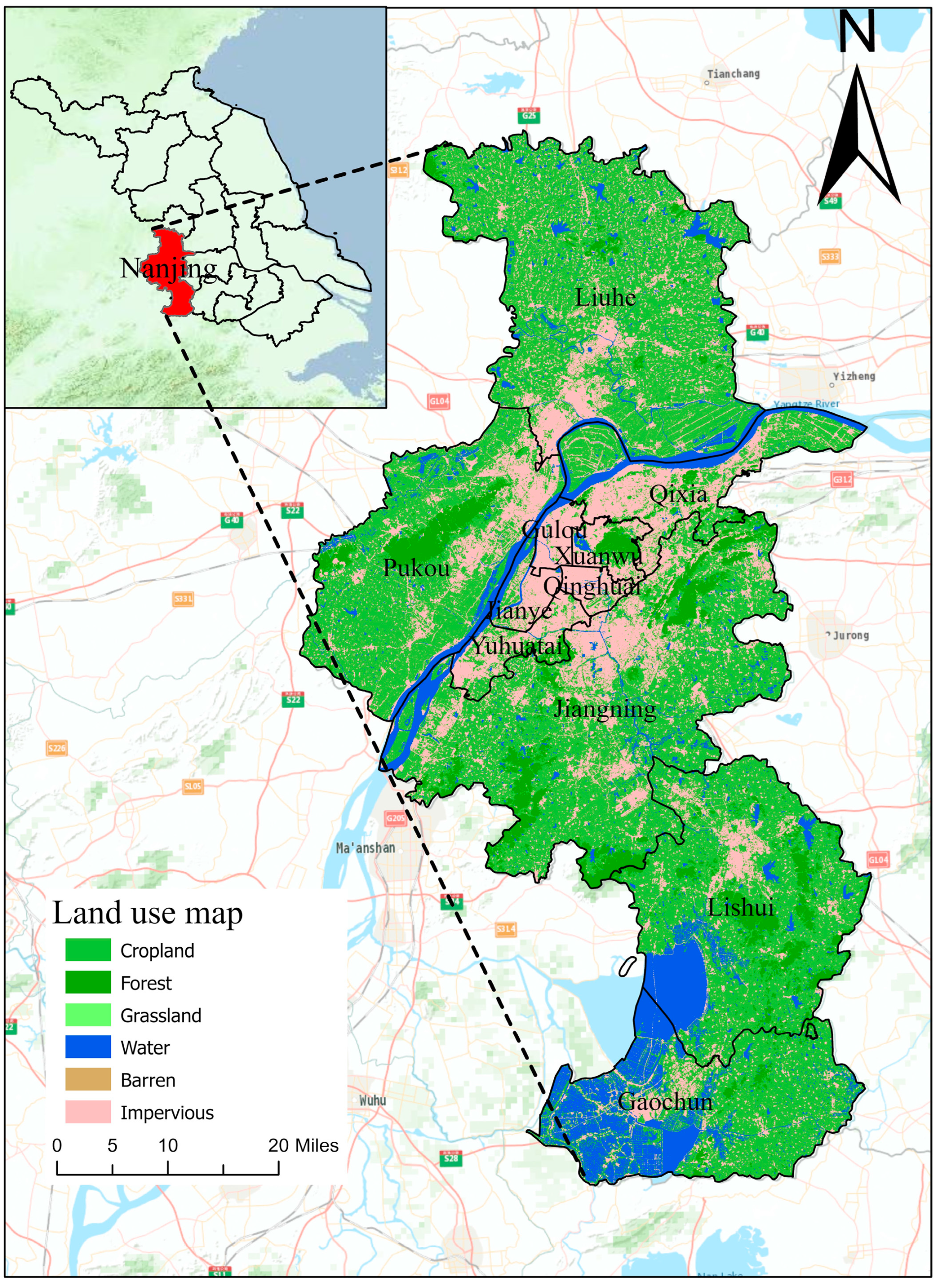
2. Study Area and Data
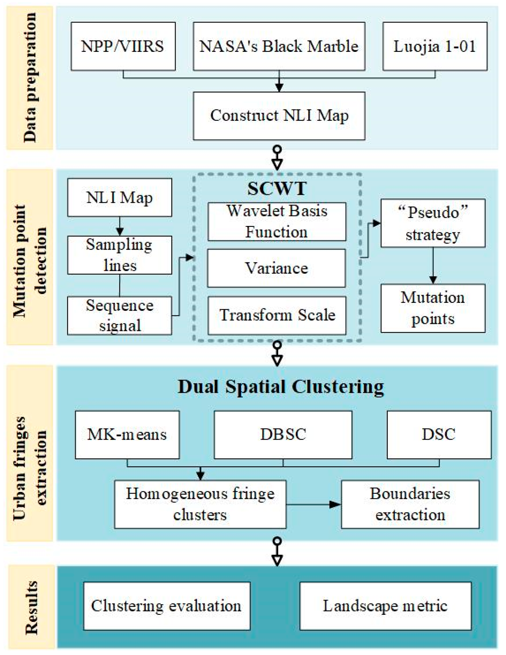
Nanjing is a significant city renowned for its high-level education institutions and transportation hub (Figure 1). It consists of eleven zones covering a total area of 6587 km2, situated in the lower reaches of the Yangtze River Delta. As of the end of 2018, the city had a registered population of 8.3 million, with 81% residing in urban areas. Nanjing’s GDP reached 960 billion yuan (approximately 140 billion USD), ranking it 10th among Chinese cities. With improvements in population growth and economic prosperity, there is a growing demand for commercial and residential space, leading to gradual development in the rural regions surrounding the city [37].
NTL includes NPP-VIIRS, Luojia 1-01 data, and NASA’s Black Marble data (Figure 2). The Luojia 1-01 data of Nanjing and its surrounding areas were obtained from the Hubei Center of High-Resolution Earth Observation System (http://59.175.109.173:8888/app/login.html, accessed on 10 July 2020), with the data distributed on 23 November 2018. The geometrically corrected products used in the study have a resolution of 130 m. To reduce the effect of light saturation, a radiometric correction for Luojia1-01 NTL was implemented using the formula L = D N 3 / 2 × 1 0 b , where D N is the digital number values of pixels and b is set to 3. We then converted the unit of Luojia 1-01 radiance to n a n o   W · cm 2 · s r 1 , which matches the unit of VIIRS data. The NPP/VIIRS data were sourced from the National Geophysical Data Center (NGDC) (https://www.ngdc.noaa.gov/eog/viirs/, accessed on 7 July 2022). In this study, the monthly averaged data from November 2018 were utilized, excluding the effects of stray light, lightning, and cloud cover, thus allowing it to reflect the spatial distribution patterns of typical NLI on the Earth’s surface. The data used in this study have a spatial resolution of 500 m. The daily Black Marble data (VNP46A2) were obtained from the NASA Level-1 and Atmosphere Archive and Distribution System Distributed Active Archive Center (LAADS DAAC) (https://blackmarble.gsfc.nasa.gov/#product, accessed on 2 September 2022). The VNP46A2 dataset, which includes daily moonlight-adjusted night-time light and population census estimates, was collected at a spatial resolution of 500 m within the temporal range of November 2018 night-time light data. Black Marble data preprocessing has been carried out according to Zheng’s work (https://github.com/qmzheng09work/NTL-VIIRS-BlackMarbleProduct). For consistent analysis and comparison across various data sources, we initially converted all the data into the Lambert Azimuthal Equal Area Projection. Subsequently, NPP-VIIRS and NASA’s Black Marble data were resampled to a spatial resolution of 500 m × 500 m (cell size) using the nearest neighbor method within the ArcGIS “Resample” tool, while Luojia 1-01 data were resampled to the same resolution using the aggregating rule within the ArcGIS “Aggregate” tool.
In the urban fringes, the NLI values typically exhibit a gradual decrease as one moves from the bright urban center to the darker and less developed rural areas. As urbanization extends outward, the NLI serves as a useful indicator of the gradual changes in human settlement and land use from urban to rural environments [8,38]. The NLI index in this study corresponds to the radiance value of each pixel derived from the NTL images. The city epicenters exhibit higher NLI indices, and the grid units are more densely populated in those areas. As one moves farther away from these centers, the NLI indices gradually decline. This results in a transition from continuous to discrete parts in terms of pixel distribution. Pixels with higher NLI indices tend to be more clustered, while those with medium-level indices are more commonly found in urban fringes. This characteristic indirectly reflects the variability of the urban fringe area. To facilitate the subsequent process of detecting mutation points using SCWT (details in Section 3.1), we converted the night-time light pixels to grid square cells and assigned the NLI index of each pixel to each grid cell (Figure 3).

3. Methodology

The identification framework consists of three main parts (Figure 4): (1) the SCWT method has been employed to identify mutation points along the gradient of the urban fringe; this helps in detecting significant changes in the spatial distribution of NLI; (2) based on the spatial distribution of mutation points, three dual spatial clustering methods have been adopted to detect homogeneous spatial fringe clusters; (3) the boundaries of the urban fringe areas were connected automatically, and the evaluation of the urban fringe was investigated via different NTL using different dual spatial clustering methods.

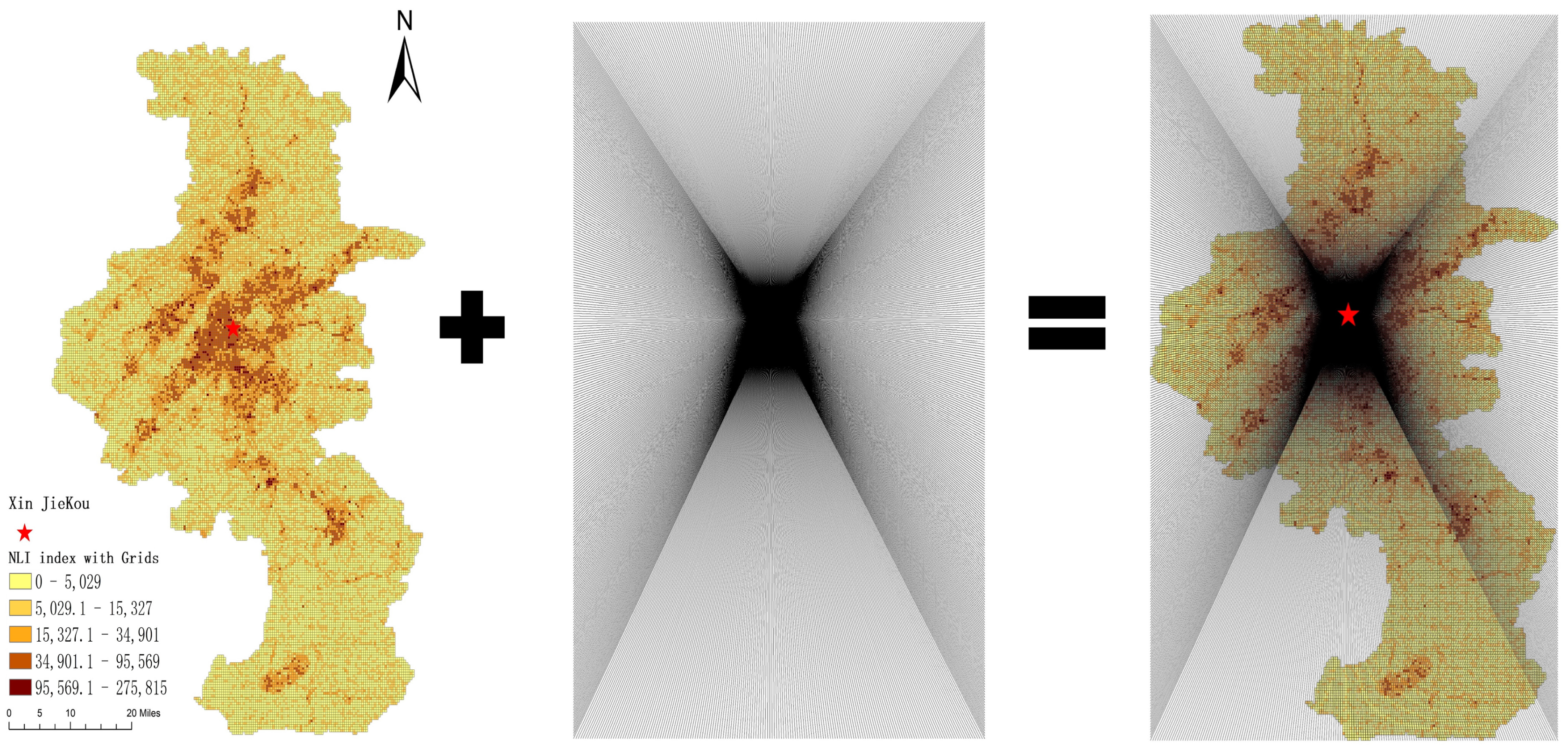
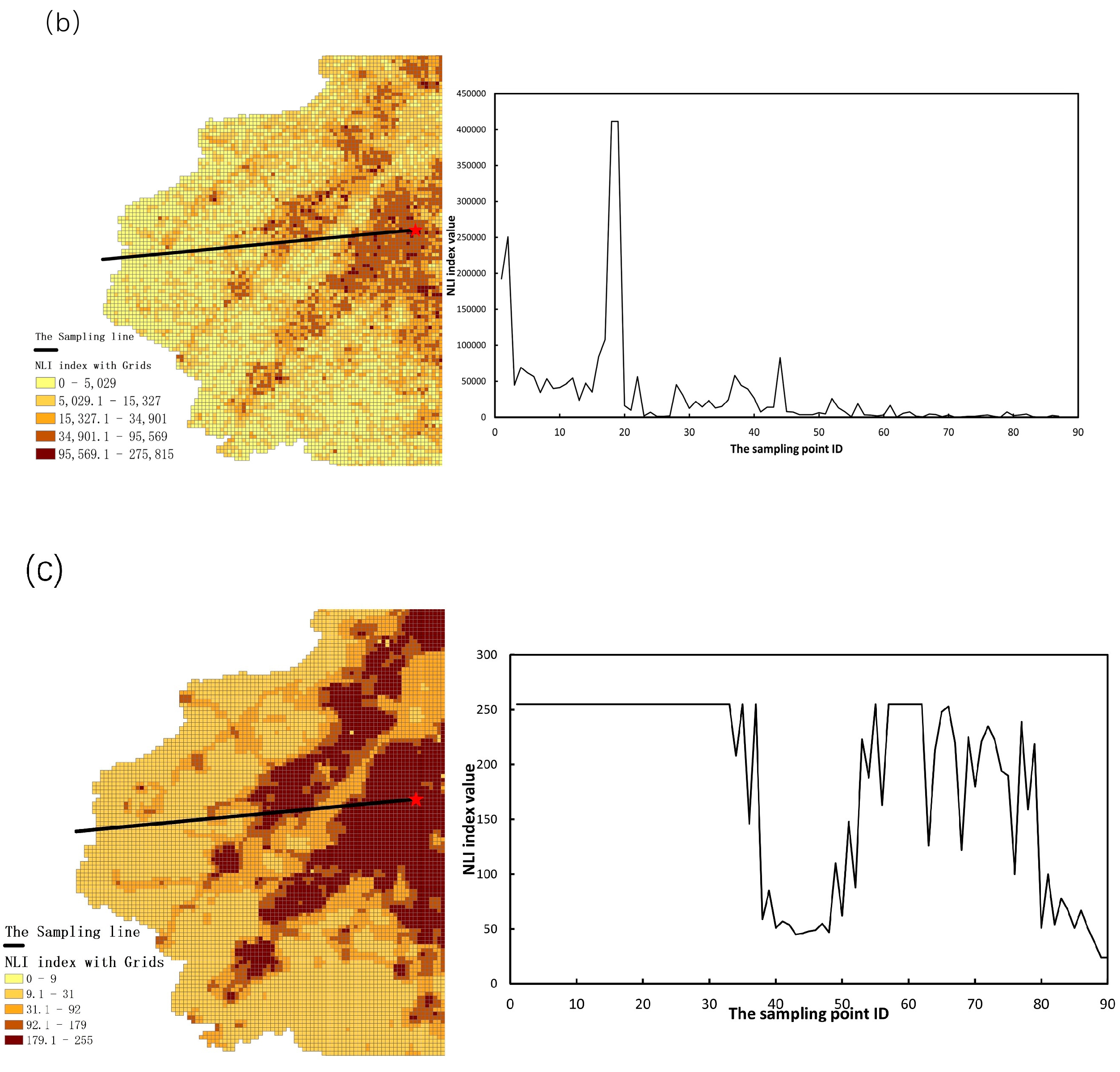
3.1. The Detection of Mutation Points Using SCWT

The SCWT method is a signal-processing technique that analyzes the frequency content of a signal at different scales and orientations. By applying the SCWT to the NLI grid map, it is possible to identify significant changes in NLI, which can serve as indicators of urban fringe boundaries or transition areas [28,30,31]. In a previous study [31], the process began with a city center as the starting point, and a one-degree interval was used to establish 360 sampling lines. Additionally, the center of the outermost grid within the entire study area was designated as the endpoint. This approach ensured the inclusion of each grid cell in the calculations. Subsequently, we constructed a spatial urbanization sequence signal for each sample line by recording the urbanization indices (the NLI index in this study) of the grids intersecting the sample line from the city center to the periphery. Following this, the mutation points of each signal, which included the maximum and minimum values, were identified using the SCWT method with the optimal scale. These mutation points were then mapped to identify the spatial locations of urbanization mutations within the study area.
The SCWT method operates on the principle of decomposing the original spatial sequence signal, using wavelet transform to obtain its approximate and detailed coefficients. The locations of significant changes in the signal, characterized by peaks and troughs in the wavelet coefficients, are identified as the “maximum modulus” points and considered as the locations of mutation points.
S C W T a , b = S x φ x = 1 a 0 L x S x φ x b a d x
In this equation, S C W T ( a , b ) denotes the wavelet coefficients, S x represents the signal of a spatial sequence, and φ x includes parameters for spatial scale ( a ) and shifting proxy ( b ), where the latter is determined by a distinctive factor of the wavelet function, denoted as scale a , which controls the extent of decomposition.
In this study, there were three steps needed in order to detect mutation points of urban fringe regions using the SCWT algorithm: first, the Db3 wavelet from the Daubechies wavelet family was selected as the wavelet basis function; second, the local maximum in the coefficients obtained from Scale = 2 was examined in the process of identifying mutation points; third, the urban fringe was objectively detected by segmenting the mutation map using k-standard deviations strategy that eliminates “pseudo” mutation points. This enhancement in the detection method ensures a more reliable and precise identification of the urban fringe [30,31] (Supplementary Materials Word File S1 provides the detailed discussions).

3.2. Extraction of Urban Fringe Based on Different Dual Spatial Clustering Methods

3.2.1. Modified k-Means Algorithm (Mk-Means)

The MK-Means method [33], which incorporates attribute clustering in addition to the K-means algorithm, considers both the spatial heterogeneity and attribute similarity (i.e., NLI index). The K-means method starts by randomly selecting k initial cluster centers, then it calculates the distance between each object and these cluster centers. A cluster is formed by assigning each object to its nearest cluster center, where the cluster centers, along with their corresponding assigned objects, constitute the cluster. The key difference between the K-means method and the dual spatial clustering algorithm lies in their definition of distance. The K-means method calculates the spatial distance of the clustering targets, while the MK-Means algorithm not only focuses on the spatial clustering of the targets but also takes into account their attribute distance. Therefore, the MK-Means algorithm uses a generalized Euclidean distance as the clustering metric, replacing the spatial distance used in the K-means method. The generalized Euclidean distance is defined as follows:
D p i , p j = w 1 D S p i , p j + w 2 D A p i , p j .
In this equation, D p i , p j between p i and p j is calculated as the weighted sum of the normalized spatial distance D S p i , p j and non-spatial distance D A p i , p j . The default values for the weights w 1 and w 2 are both set to 0.5 [35].

3.2.2. Density-Based Spatial Clustering Algorithm (DBSC)

The DBSC algorithm is a clustering method based on the adaptive Delaunay triangulation (DT) and spatial entity position constraints [32]. Its basic idea is to impose different levels and types of constraints on the edges of the Delaunay triangulation to obtain discrete spatial clusters formed by connected triangle edges and to establish neighboring relationships between spatial entities within each cluster. Subsequently, non-spatial attribute constraints are introduced to filter the clustering results, achieving dual clustering of both spatial and attribute aspects. The algorithm primarily consists of two steps:
(1)
Clustering based on spatial position constraints
Considering that urban fringes have non-uniform boundaries in terms of size and shape, the mutation points tend to be unevenly distributed. The traditional proximity relationship established by DT may result in certain errors at the edges [39]. The DBSC algorithm addresses this issue by employing a hierarchical edge-length constraint strategy that trims the edge lengths in DT.
Suppose S D B is the mutation points database, D T ( S D B ) denotes the D T of S D B , where each point P i represents a mutation point. Let G l o b a l _ M e a n ( D T ) represent the average length of all edges in D T , and L o c a l _ M e a n ( P i ) denotes the average length of all edges connected to P i . G l o b a l _ V a r i a t i o n ( D T ) denotes the standard deviation of all edge lengths in D T , and L o c a l _ V a r i a t i o n ( P i ) denotes the standard deviation of all edge lengths connected to P i . For any point P i , the global distance constraint criterion can be expressed as follows:
G l o b a l _ D i s t a n c e _ C o n s t r a i n t s ( P i ) = G l o b a l _ M e a n ( D T ) + α · G l o b a l _ S D ( D T )
α = G l o b a l _ M e a n ( D T ) L o c a l _ M e a n ( P i ) .
In D T , if the length of an edge directly connected to P i is greater than or equal to the G l o b a l _ D i s t a n c e _ C o n s t r a i n t s ( P i ) , the edge will be eliminated from D T ( S D B ) . Once the long edges have been removed at the global level, there might still be some long edges remaining at the local level. To address this, local edge length constraints are subsequently applied.
After implementing the global edge length constraint, the resulting subgraph is denoted as G i , P j is a point in G i , 2 _ o r d e r _ M e a n ( P j ) represents the average value of all edge lengths within the 2nd order neighborhood of P j , and M e a n _ V a r i a t i o n ( P j ) represents the average of variances of directly connected edges to P j . The local edge length constraint can be expressed as follows:
L o c a l _ D i s t a n c e _ C o n s t r a i n t s ( P j ) = 2 _ o r d e r _ M e a n ( P j ) + β × M e a n _ V a r i a t i o n ( P j ) .
Generally, β is set to 2. For any point P j in G i , if the length of edges within its second-order neighborhood is greater than or equal to L o c a l _ D i s t a n c e _ C o n s t r a i n t s ( P j ) , then those edges are removed from the triangulation. By applying local trimming, the spatial adjacency relationships of entities can be better determined.
(2)
Clustering based on non-spatial attribute constraints
The modified Delaunay triangulation, C-DT, is obtained after applying global and local trimming operations. Additionally, non-spatial attributes (i.e., the NLI index) are involved in the identification of spatial clusters. To facilitate the calculation of non-spatial attribute distances, the Euclidean distance is used to represent the non-spatial attribute distance of mutation points. It is denoted as D i s t ( P i , Q i ) , and a threshold T is used to represent the similarity threshold for non-spatial attributes. Before that, several definitions are provided.
Definition 1.
Spatial Neighborhood: For any mutation point P i  in C-DT, the set of spatial points that are directly connected to  P i    through shared edges forms the neighborhood of  P i , denoted as N e i g h b o r s ( P j ) .
Definition 2.
Spatially directly reachable: In C-DT, if there are two points,  P i  and  Q i , that share a common edge and satisfy the condition  D i s t P i , Q i < T ,  P i  and  Q i  are considered to be spatially directly reachable in terms of non-spatial attribute. In this case,  D i s t P i , Q i  quantifies the dissimilarity in non-spatial attribute between these two mutation points. The threshold, denoted as  T , takes into consideration the difference between the average value of a temporal cluster and the attribute value of a mutation point that will be added to the same temporal cluster.
Definition 3.
Spatially indirectly reachable: In C-DT, if there is a set of mutation points CMU (there are at least two mutation points in CMU) and satisfy the condition D i s t P i , A V G ( C M U ) < T , P i and C M U are referred to as being spatially indirectly reachable. In this case, the average value of non-spatial attribute values for all points in the CMU is represented by A V G ( C M U ) .
Definition 4.
Density Indicator: For a point P i  in C-DT, the density indictor D I ( P i ) represents the density index of P i .
D I ( P i ) = N s d r ( P i ) + N s d r ( P i ) / N ( P i ) .
N s d r ( P i ) represents the number of spatially directly reachable points from P i . N ( P i ) represents the number of points in N e i g h b o r s ( P j ) .
Definition 5.
Spatial Cluster Core: Among all unclustered mutation points, the point with the highest density indicator is referred to as the spatial cluster core. When multiple points have the maximum density indicator, the spatial cluster core is chosen based on the point with the minimum average non-spatial attribute difference among its corresponding neighboring points.
Definition 6.
Expansion Core: For any point P i   in C-DT, if there is at least one point in its neighborhood N e i g h b o r s ( P i ) that is spatially directly reachable from P i , P i   is referred to as an expansion core.
The DBSC algorithm’s specific implementation process is outlined as follows: ① Construct the DT of the mutation points and apply global-to-local hierarchical constraints to remove long edges. ② Select a spatial cluster core P i . In its neighborhood N e i g h b o r s ( P i ) , sort the expansion cores that have not been clustered based on their density index. ③ Within N e i g h b o r s ( P i ) , cluster the expansion cores that satisfy both spatially directly and indirectly reachable with P i , in descending order of density index. This forms the initial cluster. ④ Use the expansion core that has been added to the initial cluster as the new spatial cluster core and continue expanding according to the strategies in steps 2 and 3. ⑤ When there are no points that can be added to the cluster with P i as the spatial cluster core, a spatial cluster is formed. ⑥ Iterate through steps 2 to 5 until all mutation points have been traversed. Points that have not been added to any cluster are labeled as noise points.

3.2.3. DSC Algorithm

DSC aims to address the challenges of heterogeneity and noise by incorporating both spatial proximity and attribute similarity [34]. DSC initiates by employing D T with edge-length constraints, which takes into account arbitrary geometrical shapes, different densities, and spatial noise, to establish spatial proximity relationships among mutation points. Subsequently, an information entropy clustering strategy is devised to identify clusters that exhibit similar attributes. This approach enables adaptive and precise cluster detection while taking into account the existence of heterogeneity and noise.
(1)
Clustering constrained by spatial proximity
Following the construction of the DT of the mutation points, the DSC algorithm proceeded to utilize global and local proximity criteria to partition the mutation points into multiple spatial clusters. Through the application of global criteria, the long edges will be removed at the global level. This process can be expressed as follows:
G l o b a l _ L o n g E d g e s ( p ) = { e i | e i > G l o b a l M e a n + G l o b a l S D × G l o b a l M e a n P a r t i a l M e a n ( p ) } ,
where G l o b a l _ L o n g E d g e s ( p ) represents the set of long edges that need to be deleted at point p . G l o b a l M e a n refers to the average length of all edges in DT, P a r t i a l M e a n ( p ) denotes the average length of the edges directly connected to point p , and G l o b a l S D denotes the standard deviation of edge lengths in DT.
Subsequently, the local proximity constraint is implemented to remove the remaining long edges. The local process follows the following criteria:
F p = L o c a l S D p / L o c a l M e a n L e n g t h p L o c a l M e a n L e n g t h p = 1 d p i = 1 d p e i L o c a l S D p = i = 1 d p L o c a l M e a n L e n g t h p e i 2 d p ,
where L o c a l M e a n L e n g t h p represents the mean length of edges in N ( p ) , and L o c a l S D p is the standard deviation of the lengths of edges in N ( p ) . d p denotes the number of edges incident to p , and e i is the length of edges in N ( p ) . The final spatial proximity comprise all connected mutation points for which F p γ .
(2)
Clustering constrained by attribute similarity
DSC utilizes an attribute clustering method based on information entropy to classify the clustering results according to the attributes of the mutation points. The attribute entropy represents the degree of similarity between the central mutation point and the surrounding mutation points within the first-order neighborhood. It can be calculated using the following formula, where a higher value indicates a smaller difference between the central point and the connected points:
D A E n e i O = E o c n + 1 E o c = i = 1 n + 1 p i ln p i p i = v i j = 1 n + 1 v j ,
where D A E n e i ( O ) represents the attribute entropy of mutation point O , and E o c represents the attribute similarity between point O and clustering cluster C . The clustering cluster C consists of n points { C 1 , C 2 , C 3 , , C n }, where point O represents the central mutation point and cluster C is the set of mutation points within the first-order neighborhood of point O . The NLI index values of each mutation point in the cluster are denoted as { v 1 , v 2 , v 3 , , v n }, and the NLI index value of the central mutation point O is represented as v n + 1 .
After calculating the attribute entropy for each mutation point, the mutation point with the highest attribute entropy is selected as the starting point. Using Equation (9), the starting point is considered as the central point O , and each surrounding mutation point is treated as a separate clustering cluster C . The attribute similarity E o c between the central point and each surrounding point is computed. The initial clustering cluster is formed by combining the mutation point O with the highest attribute entropy and the point with the maximum attribute similarity E o c among its surroundings. The candidate points are determined as the mutation points within the first-order neighborhood of the initial clustering cluster. Equation (10) was employed to compute the E o c between each candidate point and the initial cluster:
θ = E o c E o c m a x E o c m a x = ln ( n + 1 ) ,
where θ is the standardized variable; the maximum information entropy between mutation point O and the temporal cluster C, denoted as E o c m a x , is obtained via the hypothesis that the attribute values of the mutation points within temporal cluster C are equal. When θ is great than the threshold, the mutation point O will be added into cluster C; if it exceeds the threshold, we allow the mutation point O to be added to temporal cluster C . By choosing an appropriate value for θ , the PBM index is employed to achieve favorable outcomes. Achieving a high score for the PBM index confirms the acceptability of the result in terms of the attribute entropy measurement [40].
The cluster was iteratively expanded by repeating the steps of candidate selection until the first-order neighborhood of the cluster no longer contained similar mutation points. Subsequently, the remaining mutation points in the initial cluster were evaluated based on their D A E n e i O values, and the mutation point with the highest D A E n e i O value was selected as the starting point for the second cluster. The aforementioned steps were repeated to group all mutation points into different sub-clusters.

3.3. Boundary Extraction of Homogeneous Fringe Clusters

Peethambaran and Muthuganapathy [41] proposed a Delaunay-based shape reconstruction method, which was utilized to accurately detect the boundaries of geographical phenomenon. The urban fringe comprises both outer and inner boundaries, and a significant advantage of this approach is its ability to identify both cavities and holes represented as planar points, making it well-suited for detecting fringe boundaries.

3.4. Evaluation

To evaluate the pros and cons of the different results, various quantitative validations were carried out. First, the RS index was utilized as the clustering indicator, aimed at quantifying the level of dispersion among spatial entities [42]. Second, according to Yang et al. [31] and Dai et al. [43], the three landscape pattern indices—Patch Density (PD), Landscape Shape Index (LSI), and Shannon’s Diversity Index (SHDI)—were computed to reflect the characteristics of spatial configuration and structural composition in the urban fringe area (the index calculation process was performed using FRAGSTATS 4.2 software). Landscape pattern indices were based on the land use data for Nanjing City in 2018, which was provided by Yang and Huang’s work [44]. The meanings of the evaluation indicators are presented in Table 1.

4. Results

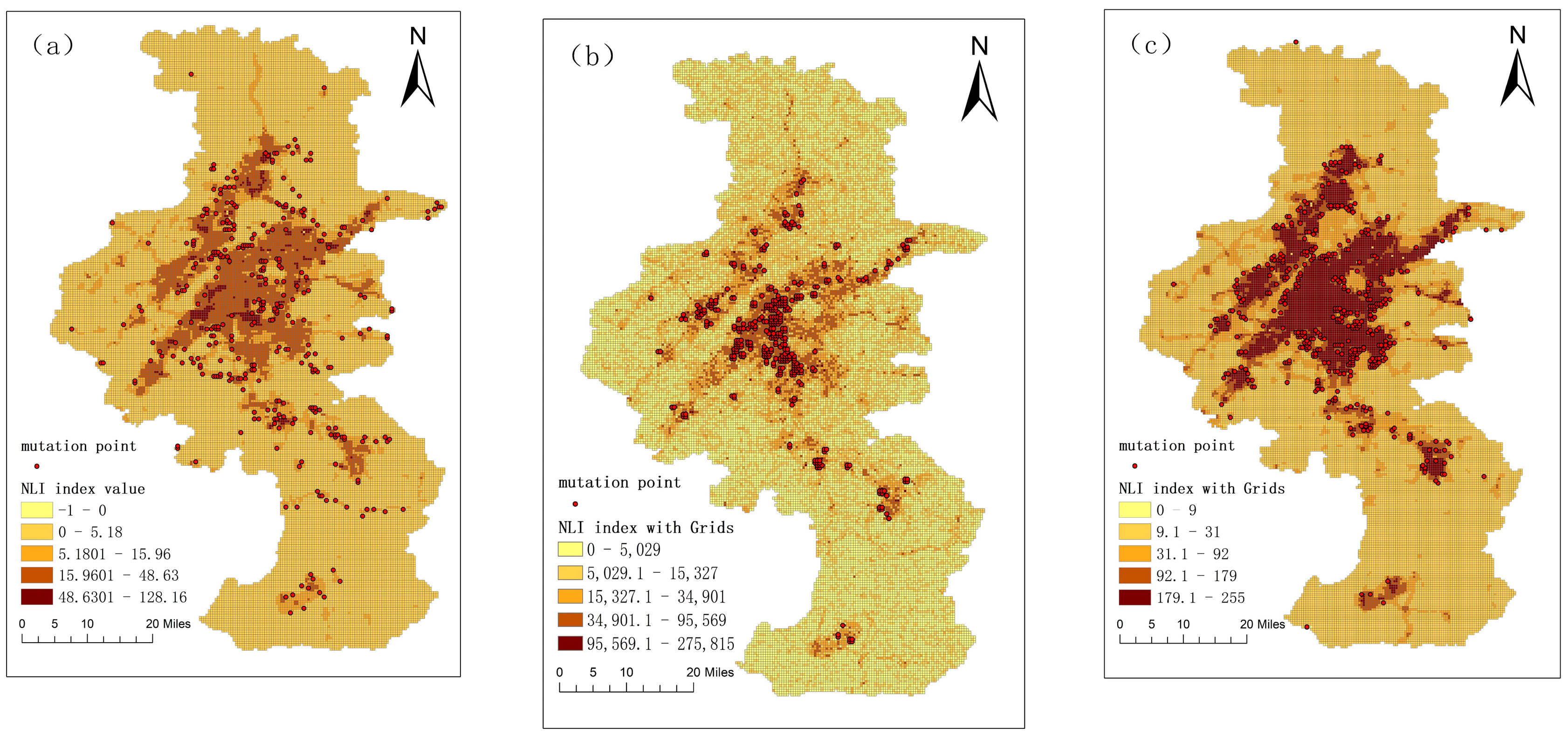
4.1. Mutation Points Detection from Different NTL Sources

According to the SCWT method described in Section 3.1, we conducted mutation detection and extracted clusters of mutation points in different NLI maps. The study began by extracting sample lines using Xinjiekou, the main center of Nanjing city, as the starting point. Furthermore, the endpoints of sample lines were extended to reach the center of the outermost grid in the entire study area. A total of 252 sample lines were generated for the center (Figure 5). Later, the NTL indices of the grids intersecting each sample line were recorded to construct the spatial sequence signal. This recording process started from the city center and extended towards the periphery.
It can be observed in Figure 6 that the example sampling lines extend from the city center to the periphery, passing through approximately two high NLI value areas. The curve demonstrated a shift from high values to low values, followed by a subsequent shift from low values back to high values. The fluctuation trend described above can be observed in spatial sequence curves for all three datasets. Furthermore, it is worth noting that the maximum values in the second high-value area are all lower than the NLI value at the city center, which was consistent with the description of urbanization in urban fringe area.
The SCWT method was utilized in this study using the optimal scale (Scale a = 2) and the db3 wavelet as the basic function for processing (as described in Section 3.1). Yhe mutation points of each signal, corresponding to the highest and lowest scores, were identified. After mapping the identified mutation points as individual points, the model applied a filtering process to eliminate “pseudo” mutation points based on two standard deviation values via a stepwise trial [30]. As a result, 329, 339, and 445 mutation points were identified in NPP/VIIRS, Luojia 1-01, and NASA’s Black Marble data, respectively, with many intersection points (Figure 7).

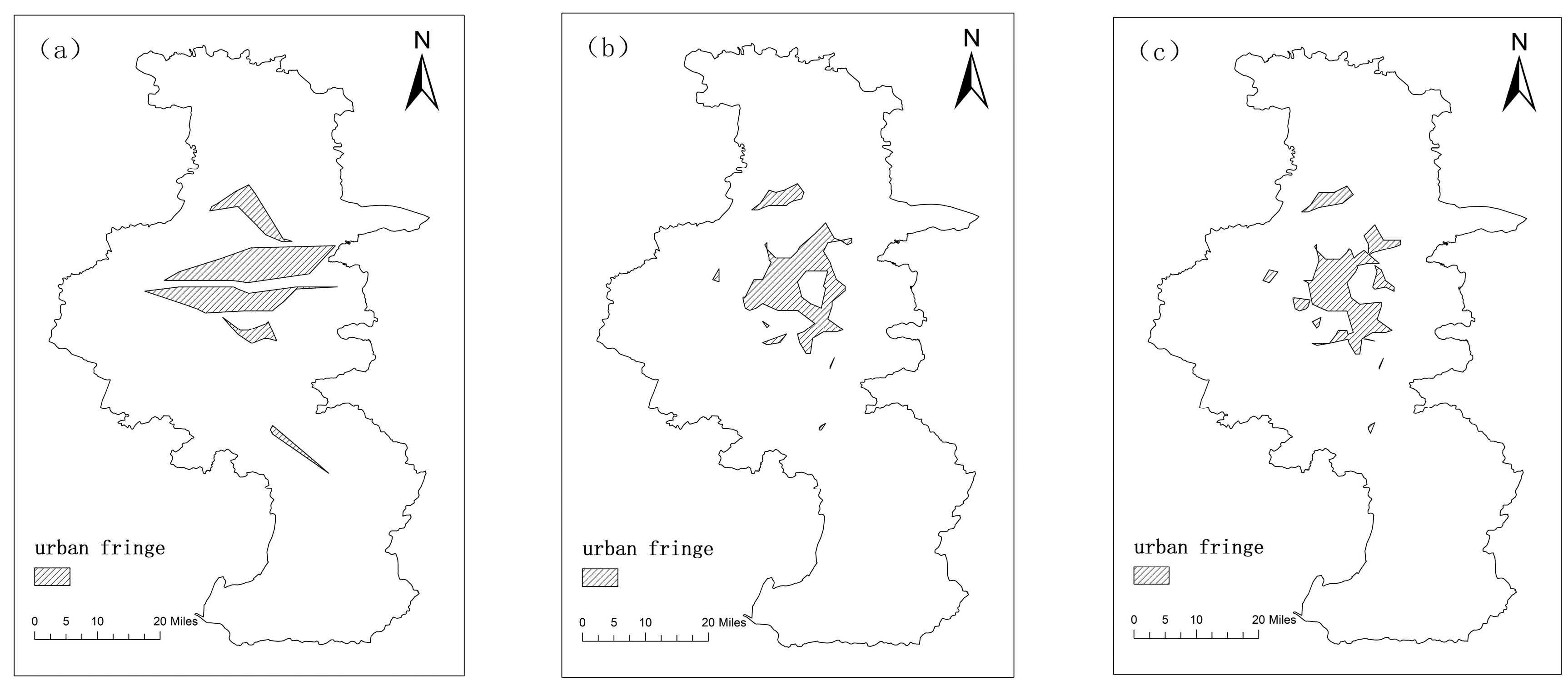
4.2. Urban Fringe Extraction by Different Dual Spatial Clustering Methods

Figure 8, Figure 9 and Figure 10 present the results obtained by applying the three dual spatial clustering algorithms to the mutation points. The points of the same color indicate that they belong to the same clusters, while the points denoted by “x” were classified as noise, indicating that their spatial locations and attribute values significantly differ from those of other mutation points in their spatial neighborhood. The basic statistical information of these clusters obtained by the different algorithms was listed in Table 2.
Regarding the clustering results of the MK-Means, DBSC, and DSC algorithms in different datasets, the MK-Means clustering results demonstrated a well-defined hierarchical structure, where the clusters exhibited a distinct “drawer-like” distribution from north to south (Figure 8). The extracted boundaries of urban fringes also exhibited the same distribution pattern (Figure 11), which, to some extent, can reflect the differences in urbanization between different regions. However, the MK-Means algorithm faces challenges in accurately identifying non-convex-shaped clusters, and its clustering results are often susceptible to the influence of noise. As a result, it may fail to detect certain adjacent spatial clusters with different attributes within the clusters, as indicated by the lowest CV values (Table 2), more scattered distribution (Figure 11), and poorer performance (see below). Compared to the MK-Means clustering, the DBSC algorithm exhibited higher accuracy in urban fringe boundary extraction. The application of DBSC yielded several clusters as well as noise in the clustering results (Figure 9). When analyzing the urban–rural fringe segments from north to south Nanjing, two main regions (i.e., Jiangbei and Zhucheng) show a concentration of more human activities at night. However, there was a considerable urban–rural fringe segment that extended from the north to the south of Nanjing (as shown in Figure 9 and Figure 12), which was inconsistent with the actual situation. This deviation was attributed to the small differences between local mutation points. DBSC fails to differentiate the actual differences between two adjacent clusters as it ignores the tendency of the NLI index. The findings suggest that the DBSC algorithm is not suitable for datasets characterized by uneven distributions of attributes. The clustering results obtained by DSC directly displayed a noticeable difference between adjacent clusters, as indicated by higher CV values compared to the ones achieved with the other methods (Table 2). Through a simple analysis of the results, it becomes evident that different neighborhoods exhibit distinct spatial patterns of mutation points while identifying the urban–rural fringe. Moreover, the influence of local spatial patterns of mutation points on density values exhibits variation across the entire density surface. Compared with the urban fringe areas results by DBSC (Figure 12b,c), the DSC algorithm is particularly effective in detecting clusters in datasets where non-spatial attributes are unevenly distributed (Figure 13b,c). However, it is important to note that several points were wrongly identified as noise, resulting in the over-segmentation of urban–rural fringes into many small ones. As shown in Figure 13b, the boundary extraction results of Luojia 1-01 data using the DSC method reveal that the urban fringe regions in the main urban area are excessively divided into multiple small fragments, as indicated by lower RS value (Figure 14).
Regarding different NTL datasets, the boundary extraction results achieved via DBSC and DSC clustering of three distinct datasets distinctly illustrated the distribution ranges of major urban fringe regions. Notably, the Xinjiekou area demonstrated a higher NLI index in comparison to its surrounding regions. This distinctive characteristic was manifested in the extracted urban fringe boundaries from all three datasets, collectively forming a void and outlining the extent of the urban region. In the extraction results of urban fringe areas using NPP/VIIRS data, there was a contiguous appearance with internal voids being covered, resulting in excessively regular patterns (Figure 12a and Figure 13a). Specifically, the extraction boundaries at the Zhucheng and Jiangbei are not satisfactory. Considering the presence of the Yangtze River, the NLI index within this basin was relatively low, leading to a correspondingly lower level of urbanization characteristics. Consequently, the urban fringe boundaries in the north and south of the Yangtze River basin were expected to exhibit a noticeable demarcation. However, in the NPP/VIIRS data, the extraction results did not capture the distinctive distribution characteristics in these two areas. This was mainly due to the prominent influence of light spillover on the extraction of fringe areas from NPP/VIIRS data, leading to the contiguous appearance of fringe areas. This is indicated by the lowest PD and SHDI values, as well as the highest LSI values (Figure 15a). Compared to the NPP and Black Marble datasets, the Luojia 1-01 has a higher spatial resolution and includes various pieces of detailed information such as roads, bridges, and streets. According to Li et al. [45], using the Luojia 1-01 data for built-up area extraction in Nanjing can yield a larger number of built-up area patches, and the fringe areas can also be well distinguished between Zhucheng and Jiangbei regions (Figure 12b and Figure 13b). However, when there were a large number of built-up area patches and fragmentation within the built-up areas, the issue of information loss in the urban fringe regions became severe. The most evident manifestation of this problem was the unsatisfactory extraction results of the fringe areas, particularly in the Zhucheng area of Nanjing and the southernmost Gaochun district, where the majority of the fringe area information is missing (Figure 12b and Figure 13b). Accordingly, using Luojia 1-01 data for urban fringe area extraction led to a significant increase in patch density, accompanied by a notable reduction in landscape fragmentation and heterogeneity (Figure 15b). The Black Marble data effectively addressed the problem of light spillover seen in the NPP/VIIRS data and significantly reduced the information loss in urban fringe regions observed in the Luojia 1-01 data. Notably, when using the Black Marble data combined with DSC clustering, the extraction of urban fringe area boundaries in Nanjing were more precise and accurate.

5. Discussion

5.1. NASA’s Black Marble and NPP/VIIRS Data Effectively Captured the Abrupt Change of Urban Fringe Areas with NTL Variations

This study employed the SCWT method to detect mutation points in individual signals. These mutation points were then mapped to identify urban fringes in Nanjing where urbanization-related changes had occurred. The city center, characterized by a high NLI index, was encompassed by mutation points, indicating significant urbanization-related mutation characteristics at the interface of the city center and fringes. Other mutation points, discretely distributed, represent the mutability in the urban fringes. As shown in Figure 6, the Xinjiekou area, the main center of Nanjing city, demonstrated a higher NLI index compared to its surrounding regions. This characteristic was manifested in the extracted urban fringe boundaries from all three datasets (Figure 13 and Figure 14). However, for other mutation points, Luojia 1-01 did not yield satisfactory results, as the distribution was relatively concentrated (Figure 9b and Figure 10b). Compared to the NPP-VIIRS and Black Marble data, the Luojia 1-01 data requires radiance calibration using the formula L = D N 3 / 2 × 1 0 b (where b is usually set to 10). When b is set to high value, the variance of the NLI value with grids will be correspondingly smaller. The brightness of night-time lights was not significantly different. Therefore, the limited number of detected mutation points hinders the precise representation of urban fringe area boundaries. In Figure 16 ( b = 10 ) and Figure S1 (see Supplementary Materials), it can be observed that most of the mutation points are distributed in the city center area, and no mutations were identified in the Gaochun district.
We iteratively experimented with b from 0 to 10 m (step size = 1). As the b value increased from 0 to 10, the number of mutation points continued to decrease, but they were still predominantly concentrated around the Xinjiekou area. Finally, the optimal parameters ( b = 3 ) in this study will be defined when the RS index achieves the maximum value in cluster process.

5.2. DSC Provided a Reliable Approach for Accurately Extracting Urban Fringe Area Using NASA’s Black Marble Data

In this study, the urban fringe exhibits high spatial heterogeneity in urbanization, with an uneven distribution of NLI. DSC is based on the assumption that the NLI in the urban fringe is more heterogeneous compared to that in urban and rural areas. The DSC clustering results revealed a clear difference between adjacent clusters, as indicated by higher CV values compared to the ones achieved with the other methods. In addition, a better representation of NTL variation details inside urban areas was key to mapping urban fringe areas. NASA’s Black Marble data can provide more detailed information about intracity NTL variations, which was previously less achievable with VIIRS data [10]. As depicted in Figure 10c and Figure 14c, the combination of Black Marble data with DSC clustering effectively extracted the urban fringe boundaries in Nanjing, offering valuable insights into localized variations. For example, the fringe areas between Zhucheng and Jiangbei regions can be clearly distinguished; the Purple Mountain area can also be identified, as indicated by a lower NLI index compared to its surrounding regions; in the case of Gaochun, which serves as the district center with higher urbanization, it displayed the distinct characteristics of the urban fringe. Therefore, Gaochun has been accurately recognized as an urban area and urban fringe using the Black Marble data.

6. Conclusions

In this study, we assessed three representative dual spatial approaches (i.e., MK-means, DBSC, and DSC methods) for delineating urban fringe areas using the NPP/VIIRS, NASA’s Black Marble, and Luojia 1-01 night-time light datasets. Considering Nanjing city as the study area, we used RS, PD, LSI, and SHDI to compare the results obtained from different comparative methods based on various NTL data sources. The main conclusions are as follows:
(1)
For different algorithms, the MK-Means clustering approach offers a useful perspective on the hierarchical structure and general urbanization differences between regions. However, it fails to detect certain adjacent spatial clusters with different attributes within the clusters, as indicated by more scattered distribution and poorer performance. DBSC fails to differentiate the actual differences between two adjacent clusters as it ignores the tendency of the NLI index. The urban fringe boundaries in the north and south of the Yangtze River basin (i.e., Zhucheng and Jiangbei) are not anticipated to demonstrate a distinct demarcation. The DSC algorithm is suitable for detecting clusters in datasets with an uneven distribution of non-spatial attributes. However, it resulted in the over-segmentation of urban–rural fringes into numerous smaller areas.
(2)
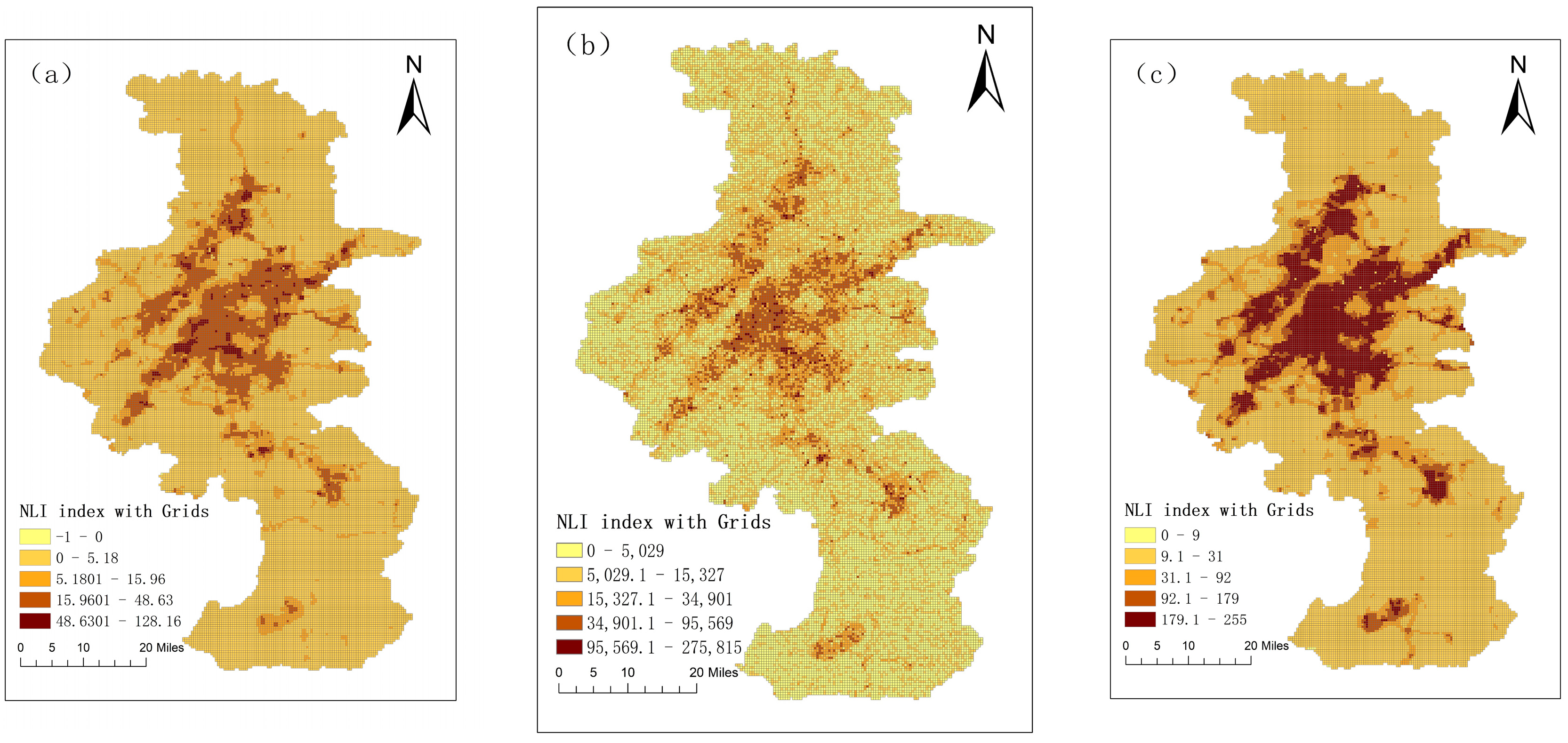
For different NTL datasets, the extraction results from NPP/VIIRS data are significantly affected by the light spillover phenomenon, leading to an overestimation of the recognition results with a high concentration of contiguous patches. Luojia 1-01 data did not yield satisfactory results due to a relatively concentrated distribution of mutation points, resulting in a significant amount of missing fringe area information, which could potentially lead to an underestimation of the recognition results. NASA’s Black Marble data with medium and high spatial resolution can better reveal inner-city NTL variations, which can offer valuable insights into localized variations to map urban fringe areas. Notably, when using the Black Marble data combined with DSC clustering, the extraction of urban fringe area boundaries in Nanjing were more precise and accurate.
There remain certain limitations that require further attention and resolution. First, recent advancements in NTL platforms have led to enriched NTL data products, providing a wide range of spatial and temporal resolutions. In future studies, it is crucial to focus on integrating multi-source NTL data to improve the achievable spatial and spectral details in urban fringe identification. Second, it is crucial to note that our study focused solely on identifying the urban fringe for a specific year. The urban fringe undergoes continuous movement towards the periphery of the city, resulting in a highly dynamic and instantaneous location. To gain a deeper understanding and address this dynamic nature, further research should involve a comprehensive analysis using long time series data. Third, it is important to note that while the identification results were confirmed through clustering evaluation and landscape pattern analysis, the verification process was limited in scope and simplicity, lacking a more comprehensive and detailed evaluation.

Supplementary Materials

The following supporting information can be downloaded at https://www.mdpi.com/article/10.3390/ijgi12100408/s1: Figure S1: Mutation Points; Word File S1: The SCWT method details [46,47].

Author Contributions

Jie Zhu and Jiaming Na conceived and designed the experiments; Ziqi Lang and Mengyao Zhu performed the experiments and wrote the paper; Shu Wang and Jiazhu Zheng contributed to discussions and validation. All authors have read and agreed to the published version of the manuscript.

Funding

This research was funded by the National Natural Science Foundation of China (Grant No. 42101430), the Ministry of education of Humanities and Social Science project (Grant No. 22YJCZH130), the Foundation of Anhui Province Key Laboratory of Physical Geographic Environment (Grant No. 2022PGE006), the Natural Resource Science and Technology Plan Project supported by Natural Resources Department of Jiangsu Province (Grant No. 2023005), and the Foundation of Key Lab of Virtual Geographic Environment (Nanjing Normal University), Ministry of Education (Grant No. 2020VGE04).

Data Availability Statement

The Luojia 1-01 night-time light imagery of Nanjing and its surrounding areas was obtained from the Hubei Center of High-Resolution Earth Observation System (http://59.175.109.173:8888/app/login.html, accessed on 10 July 2020), with the data distributed on 23 November 2018. The NPP/VIIRS data were sourced from the National Geophysical Data Center (NGDC) in the United States (https://www.ngdc.noaa.gov/eog/viirs/, accessed on 7 July 2022). The daily Black Marble data (VNP46A2) were obtained from the NASA Level-1 and Atmosphere Archive and Distribution System Distributed Active Archive Center (LAADS DAAC) (https://blackmarble.gsfc.nasa.gov/#product, accessed on 2 September 2022).

Acknowledgments

The authors declare that they have no known competing financial interests or personal relationships that could have appeared to influence the work reported in this paper.

Conflicts of Interest

The authors declare no conflict of interest.

References

  1. Liu, X.; Huang, Y.; Xu, X.; Li, X.; Li, X.; Ciais, P.; Lin, P.; Gong, K.; Ziegler, A.D.; Chen, A.; et al. High-spatiotemporal-resolution mapping of global urban change from 1985 to 2015. Nat. Sustain. 2020, 3, 564–570. [Google Scholar] [CrossRef]
  2. United Nations. World Urbanization Prospects: The 2018 Revision; United Nations Department of Economic and Social Affairs: New York, NY, USA, 2018. [Google Scholar]
  3. Gant, R.; Robinson, G.; Fazal, S. Land-use change in the ‘edgelands’: Policies and pressures in London’s rural–urban fringe. Land Use Policy 2011, 28, 266–279. [Google Scholar] [CrossRef]
  4. Peng, J.; Hu, Y.; Liu, Y.; Ma, J.; Zhao, S. A new approach for urban-rural fringe identification: Integrating impervious surface area and spatial continuous wavelet transform. Landsc. Urban Plan 2018, 175, 72–79. [Google Scholar] [CrossRef]
  5. Zhao, P.; Zhang, M. Informal suburbanization in Beijing: An investigation of informal gated communities on the urban fringe. Habitat Int. 2018, 77, 130–142. [Google Scholar] [CrossRef]
  6. Lyu, Y.; Wang, M.; Zou, Y.; Wu, C. Mapping trade-offs among urban fringe land use functions to accurately support spatial planning. Sci. Total Environ. 2022, 802, 149915. [Google Scholar] [CrossRef]
  7. Zhou, Y.; Smith, S.; Zhao, K.; Imhoff, M.; Thomson, A.; Bond-Lamberty, B.; Elvidge, C. A global map of urban extent from nightlights. Environ. Res. Lett. 2015, 10, 054011. [Google Scholar] [CrossRef]
  8. Yang, Y.; Ma, M.; Tan, C.; Li, W. Spatial Recognition of the Urban-Rural Fringe of Beijing Using DMSP/OLS Nighttime Light Data. Remote Sens. 2017, 9, 114. [Google Scholar] [CrossRef]
  9. Feng, Z.; Peng, J.; Wu, J. Using DMSP/OLS nighttime light data and K–means method to identify urban–rural fringe of megacities. Habitat Int. 2020, 103, 102227. [Google Scholar] [CrossRef]
  10. Zheng, Q.; Seto, K.; Zhou, Y.; You, S.; Weng, Q. Nighttime light remote sensing for urban applications: Progress, challenges, and prospects. ISPRS J. Photogramm. Remote Sens. 2023, 202, 125–141. [Google Scholar] [CrossRef]
  11. Elvidge, C.; Baugh, K.; Kihn, E.; Kroehl, H.; Davis, E. Mapping city lights with nighttime data from the DMSP operational linescan system. Photogramm. Eng. Remote Sens. 1997, 63, 727–734. [Google Scholar]
  12. Wang, Z.; Rom’an, M.; Kalb, V.; Miller, S.; Zhang, J.; Shrestha, R. Quantifying uncertainties in nighttime light retrievals from Suomi-NPP and NOAA-20 VIIRS Day/Night Band data. Remote Sens. Environ. 2021, 263, 112557. [Google Scholar] [CrossRef]
  13. Sanchez de Miguel, A.; Kyba, C.; Aube, M.; Zamorano, J.; Cardiel, N.; Tapia, C.; Gaston, K. Colour remote sensing of the impact of artiffcial light at night (I): The potential of the International Space Station and other DSLR-based platforms. Remote Sens. Environ. 2019, 224, 92–103. [Google Scholar] [CrossRef]
  14. Li, X.; Li, X.; Li, D.; He, X.; Jendryke, M. A preliminary investigation of Luojia-1 night-time light imagery. Remote Sens. Lett. 2019, 10, 526–535. [Google Scholar] [CrossRef]
  15. Zheng, Q.; Weng, Q.; Huang, L.; Wang, K.; Deng, J.; Jiang, R.; Gan, M. A new source of multi-spectral high spatial resolution night-time light imagery—JL1-3B. Remote Sens. Environ. 2018, 215, 300–312. [Google Scholar] [CrossRef]
  16. Lin, Z.; Jiao, W.; Liu, H.; Long, T.; Liu, Y.; Wei, S.; Liu, M. Modelling the public perception of urban public space lighting based on SDGSAT-1 glimmer imagery. Sustain. Cities Soc. 2022, 88, 104272. [Google Scholar] [CrossRef]
  17. Zheng, Q.; Weng, Q.; Wang, K. Developing a new cross-sensor calibration model for DMSP-OLS and Suomi-NPP VIIRS night-light imageries. ISPRS J. Photogramm. Remote Sens. 2019, 153, 36–47. [Google Scholar] [CrossRef]
  18. Li, X.; Li, D.; Xu, H.; Wu, C. Intercalibration between DMSP/OLS and VIIRS night- time light images to evaluate city light dynamics of Syria’s major human settlement during Syrian Civil War. Int. J. Remote Sens. 2017, 38, 5934–5951. [Google Scholar] [CrossRef]
  19. Elvidge, C.; Baugh, K.; Zhizhin, M.; Hsu, F. Why VIIRS data are superior to DMSP for mapping nighttime lights. Proc. Asia-Pacifc Adv. Netw. 2013, 35, 62. [Google Scholar] [CrossRef]
  20. Elvidge, C.; Baugh, K.; Zhizhin, M.; Hsu, F.; Ghosh, T. VIIRS night-time lights. Int. J. Remote Sens. 2017, 38, 5860–5879. [Google Scholar] [CrossRef]
  21. Roman, M.; Wang, Z.; Sun, Q.; Kalb, V.; Miller, S.; Molthan, A.; Masuoka, E. NASA’s Black Marble nighttime lights product suite. Remote Sens. Environ. 2018, 210, 113–143. [Google Scholar] [CrossRef]
  22. Wang, Z.; Shrestha, R.; Roma´n, M.; Kalb, V. NASA’s black marble multi- angle nighttime lights temporal composites. IEEE Geosci. Rem. Sens. Lett. 2022, 19, 1–5. [Google Scholar]
  23. Li, T.; Zhu, Z.; Wang, Z.; Román, M.O.; Kalb, V.L.; Zhao, Y. Continuous monitoring of nighttime light changes based on daily NASAʹs Black Marble product suite. Remote Sens. Environ. 2022, 282, 113269. [Google Scholar] [CrossRef]
  24. Masek, J.G.; Lindsay, F.E.; Goward, S.N. Dynamics of urban growth in the Washington DC metropolitan area, 1973–1996, from Landsat observations. Int. J. Remote Sens. 2000, 21, 3473–3486. [Google Scholar] [CrossRef]
  25. Wang, X.; Li, X.; Feng, Z.; Fang, Y. Methods on defining the urban fringe area of Beijing. In Proceedings of the International Symposium on Digital Earth International Society for Optics and Photonics, Beijing, China, 3 November 2010; Volume 7840. [Google Scholar]
  26. Imhoff, M.; Zhang, P.; Wolfe, R.; Bounoua, L. Remote sensing of the urban heat island effect across biomes in the continental USA. Remote Sens. Environ. 2010, 114, 504–513. [Google Scholar] [CrossRef]
  27. Qian, J.; Zhou, Y.; Yang, X. Confirmation of urban fringe area based on remote sensing and message entropy: A case study of Jingzhou, Hubei Province. Resour. Environ. 2007, 16, 451–455. (In Chinese) [Google Scholar]
  28. Peng, J.; Zhao, S.; Liu, Y.; Tian, L. Identifying the urbanrural fringe using wavelet transform and kernel density estimation: A case study in beijing city, China. Environ. Model. Softw. 2016, 83, 286–302. [Google Scholar] [CrossRef]
  29. Zhou, Y.; Smith, S.; Elvidge, C.; Zhao, K.; Thomson, A.; Imhoff, M. A cluster-based method to map urban area from DMSP/OLS nightlights. Remote Sens. Environ. 2014, 147, 173–185. [Google Scholar] [CrossRef]
  30. Zhu, J.; Lang, Z.; Yang, J.; Wang, M.; Zheng, J.; Na, J. Integrating Spatial Heterogeneity to Identify the Urban Fringe Area Based on NPP/VIIRS Nighttime Light Data and Dual Spatial Clustering. Remote Sens. 2022, 14, 6126. [Google Scholar] [CrossRef]
  31. Yang, J.; Dong, J.; Sun, Y.; Zhu, J.; Huang, Y.; Yang, S. A constraint-based approach for identifying the urban–rural fringe of polycentric cities using multi-sourced data. Int. J. Geogr. Sci. 2021, 36, 114–136. [Google Scholar] [CrossRef]
  32. Liu, Q.L.; Deng, M.; Shi, Y.; Wang, J.Q. A density-based spatial clustering algorithm considering both spatial proximity and attribute similarity. Comput. Geosci. 2012, 46, 296–309. [Google Scholar] [CrossRef]
  33. Lin, C.; Liu, K.; Chen, M. Dual clustering: Integrating data clustering over optimization and constraint domains. IEEE T. Knowl. Data En. 2005, 17, 628–637. [Google Scholar]
  34. Zhu, J.; Zheng, J.; Di, S.; Wang, S.; Yang, J. A dual spatial clustering method in the presence of heterogeneity and noise. Trans. GIS 2020, 24, 1799–1826. [Google Scholar] [CrossRef]
  35. Liu, Y.; Wang, X.; Liu, D.; Liu, L. An adaptive dual clustering algorithm based on hierarchical structure: A case study of settlement zoning. Trans. GIS 2017, 21, 916–933. [Google Scholar] [CrossRef]
  36. Zhu, J.; Sun, Y. Building an Urban Spatial Structure from Urban Land Use Data: An Example Using Automated Recognition of the City Centre. ISPRS Int. J. Geo-Inf. 2017, 6, 122. [Google Scholar] [CrossRef]
  37. Gao, C.; Feng, Y.; Tong, X.; Lei, Z.K.; Chen, S.R.; Zhai, S.T. Modeling urban growth using spatially heterogeneous cellular automata models: Comparison of spatial lag, spatial error and GWR. Comput. Enviro. Urban 2020, 81, 101459. [Google Scholar] [CrossRef]
  38. Li, J.; Peng, B.; Liu, S.; Ye, H.; Zhang, Z.; Nie, X. An accurate fringe extraction model of small-and medium-sized urban areas using multi-source data. Front. Environ. Sci. 2023, 11, 1118953. [Google Scholar] [CrossRef]
  39. Estivill-Castro, V.; Lee, I. Argument free clustering for large spatial point-data sets via boundary extraction from Delaunay Diagram. Comput. Environ. Urban 2002, 6, 315–334. [Google Scholar] [CrossRef]
  40. Pakhira, M.K.; Bandyopadhyay, S.; Maulik, U. Validity index for crisp and fuzzy clusters. Pattern Recognit. 2004, 37, 487–501. [Google Scholar] [CrossRef]
  41. Peethambaran, J.; Muthuganapathy, R. A non-parametric approach to shape reconstruction from planar point sets through Delaunay filtering. Comput. Aided Des. 2015, 62, 164–175. [Google Scholar] [CrossRef]
  42. Halkidi, M.; Batistakis, Y.; Vazirgiannis, M. Clustering validity checking methods: Part II. ACM Sigmod Rec. 2002, 31, 19–27. [Google Scholar] [CrossRef]
  43. Dai, J.; Dong, J.; Yang, S.; Sun, Y. Identification method of urban fringe area based on spatial mutation characteristics. J. Geo-Inf. Sci. 2021, 23, 1401–1421. [Google Scholar]
  44. Yang, J.; Huang, X. The 30 m annual land cover dataset and its dynamics in China from 1990 to 2019. Earth Syst. Sci. Data 2021, 13, 3907–3925. [Google Scholar] [CrossRef]
  45. Li, F.; Yan, Q.; Zou, Y.; Liu, B. Extraction Accuracy of Urban Built-up Area Based on Nighttime Light Data and POI: A Case Study of Luojia 1-01 and NPP/VIIRS Nighttime Light Images. Geomat. Inf. Sci. Wuhan University 2021, 46, 825–835. [Google Scholar]
  46. Fagan, W.F.; Fortin, M.J.; Soykan, C. Integrating edge detection and dynamic modeling in quantitative analyses of eco-logical boundaries. BioScience 2003, 53, 730–738. [Google Scholar] [CrossRef]
  47. Mallet, S. A Wavelet Tour of Signal Processing: The Sparse Way, 3rd ed.; Academic Press: New York, NY, USA, 2008. [Google Scholar]
Figure 1. Location and land use of the study area.
Ijgi 12 00408 g001
Figure 2. NTL data of Nanjing city: (a) NPP/VIIRS data; (b) Luojia 1-01 data; (c) NASA’s Black Marble data.
Ijgi 12 00408 g002
Figure 3. The NLI index at 500 m grid scale: (a) NPP/VIIRS data; (b) Luojia 1-01 data; (c) NASA’s Black Marble data.
Ijgi 12 00408 g003
Figure 4. The identification framework.
Ijgi 12 00408 g004
Figure 5. Detecting the mutation points by the sampling lines in 360 orientations (NPP/VIIRS Example).
Ijgi 12 00408 g005
Figure 6. The spatial sequence curve of the NLI index along the sampling line: (a) NPP/VIIRS data; (b) Luojia 1-01 data; (c) NASA’s Black Marble data.
Ijgi 12 00408 g006aIjgi 12 00408 g006b
Figure 7. Identification of the mutation points in the urban fringe: (a) NPP/VIIRS data; (b) Luojia 1-01 data; (c) NASA’s Black Marble data.
Ijgi 12 00408 g007
Figure 8. The MK-Means clustering results: (a) NPP/VIIRS data; (b) Luojia 1-01 data; (c) NASA’s Black Marble data.
Ijgi 12 00408 g008
Figure 9. The DBSC clustering results: (a) NPP/VIIRS data; (b) Luojia 1-01 data; (c) NASA’s Black Marble data.
Ijgi 12 00408 g009
Figure 10. The DSC clustering results: (a) NPP/VIIRS data; (b) Luojia 1-01 data; (c) NASA’s Black Marble data.
Ijgi 12 00408 g010
Figure 11. Urban fringes detection using MK-Means: (a) NPP/VIIRS data; (b) Luojia 1-01 data; (c) NASA’s Black Marble data.
Ijgi 12 00408 g011
Figure 12. Urban fringes detection using DBSC: (a) NPP/VIIRS data; (b) Luojia 1-01 data; (c) NASA’s Black Marble data.
Ijgi 12 00408 g012
Figure 13. Urban fringes detection using DSC: (a) NPP/VIIRS data; (b) Luojia 1-01 data; (c) NASA’s Black Marble data.
Ijgi 12 00408 g013
Figure 14. RS index of clustering results with various approaches.
Ijgi 12 00408 g014
Figure 15. Landscape pattern indices of urban fringe with different methods: (a) NPP/VIIRS data; (b) Luojia 1-01 data; (c) NASA’s Black Marble data.
Ijgi 12 00408 g015
Figure 16. Detection of urban fringe with b = 10: (a) MK-Means; (b) DBSC; (c) DSC.
Ijgi 12 00408 g016
Table 1. Evaluation indicators.
TypeIndicatorConnotation
Clustering
evaluation
R S = i = 1 N ( x i x ¯ ) 2 i = 1 N C j = 1 N i ( x j v i ) 2 i = 1 N ( x i x ¯ ) 2
N represents the number of entities in the dataset, N c represents the number of clusters, N i denotes the number of entities in cluster C i , v i represents the centroid of cluster C i , and x ¯ represents the centroid of the dataset.
The RS index value ranges between 0 and 1, where 0 indicates no difference between clusters, while 1 indicates significant differences between clusters.
Landscape pattern P D = 1000000 n i A
A represents the total area of the landscape type, and n i represents the total number of patches for the i t h landscape type.
PD represents the quantity of specific land use patches within a given area. It serves as a comparative metric for landscapes of varying sizes and plays a crucial role in describing landscape fragmentation. A higher P D value indicates a higher degree of landscape fragmentation.
L S I = 0.25 E A
E represents the total length of the boundaries of a specific land use type, while A represents the total area of that land use type.
The LSI can indicate the complexity of patches, which comprehensively reflects the size and heterogeneity of land classes. The LSI has a range of values from 1 to ∞, where a higher value indicates a more irregular patch shape.
S H D I = i = 1 m P i ln P i
P i represents the proportion of type   i within the entire landscape, and m represents the total number of landscape types, ranging from [0, ∞).
The SHDI is a metric that measures the complexity and heterogeneity of different types of patches within a landscape. When m = 1 , the SHDI is 0, indicating that the region has only one type of patch. As SHDI increases, it tends to be a more uniform distribution of different patch types throughout the landscape.
Table 2. Statistical information of clustering results.
NTL DataAlgorithmsStatistical Information
NCNNMEANVSDMVCV
Luojia 1-01MK-Means7015,844.3726199.3540.391
DBSC244417,281.49227,256.4391.577
DSC333731,146.35978,428.9492.518
NPP/VIIRSMK-Means704.4370.7540.168
DBSC6152.9200.7040.241
DSC131616.01218.0271.126
NASA’s Black MarbleMK-Means70131.93314.7710.112
DBSC2917175.54067.5170.385
DSC342398.67466.5540.674
Note: NC is number of clusters; NN is number of noises; MEANV is mean values of clusters, SDMV is standard deviation of mean values of clusters; and CV is the clusters’ coefficient of variation.
Disclaimer/Publisher’s Note: The statements, opinions and data contained in all publications are solely those of the individual author(s) and contributor(s) and not of MDPI and/or the editor(s). MDPI and/or the editor(s) disclaim responsibility for any injury to people or property resulting from any ideas, methods, instructions or products referred to in the content.

