Estimation of a Fundamental Diagram with Heterogeneous Data Sources: Experimentation in the City of Santander

Abstract

The reduction of urban congestion represents one of the main challenges for increasing sustainability. This implies the necessity to increase our knowledge of urban mobility and traffic. The fundamental diagram (FD) is a possible tool for analyzing the traffic conditions on an urban road link. FD is commonly associated with the links of a transport network, but it has recently been extended to the whole transport network and named the network macroscopic fundamental diagram (NMFD). When used at the link or network level, the FD is important for supporting the simulation, design, planning, and control of the transport system. Recently, floating car data (FCD), which are based on vehicles’ trajectories using GPS, are able to provide the trajectories of a number of vehicles circulating on the network. The objective of this paper is to integrate FCD with traffic data obtained from traditional loop-detector technology for building FDs. Its research contribution concerns the proposal of a methodology for the extraction of speed data from taxi FCD, corresponding to a specific link section, and the calibration of FDs from FCD and loop detector data. The methodology has been applied to a real case in the city of Santander. The first results presented are encouraging, supporting the paper’s thesis that FCD can be integrated with data obtained from loop detectors to build FD.

1. Introduction

The reduction of urban congestion represents one of the main challenges for increasing sustainability. This implies the necessity to increase our knowledge of urban mobility and traffic [1].

Mobility analysis and forecasting in urban transport systems require the building of transport supply and travel demand models. Model building takes place through a trial-and-error procedure of specification, calibration, and validation. In order to obtain models that are able to adequately reproduce the real phenomenon, two components are required: the availability of reliable and continuous mobility data over time, and the analyst’s experience regarding the specification-validation-calibration procedure. The two components must both be present; for example, big data are a precious source of information but without the construction of models they do not provide useful results in forecasted scenarios totally different from the current scenario.

Observed data related to transport systems that are obtainable via monitoring can be subdivided into two categories: data detected at one particular point (e.g., a section), and data detected in a space (e.g., a path). Monitoring systems provide data with different characteristics and with different levels of reliability in space and time.

The flow-density function is commonly known as a fundamental diagram, or FD. The FD is associated with the links of the transport network, and it has recently been extended to the area or to the transport network level known as the network macroscopic fundamental diagram, or NMFD. At the link or network level, the FD is important for supporting the simulation, design, planning, and control of the urban transport system [2].

The building of supply models through road transport networks requires the specification and calibration validation of flow-density function in relation to the geometric and functional characteristics of road infrastructures (links and nodes).

The monitoring systems that are commonly used are based on loop detectors. Recently, floating car data (FCD), based on vehicles’ trajectories and obtained using GPS devices, have been used. The loop detectors provide traffic data for one point of the link and also continuously over time. FCD generally provide information on a sample of vehicles selected according to specific criteria (e.g., vehicles equipped with GPS provided by insurance companies), and then extend this to the total fleet of vehicles. Therefore, it is necessary to integrate the two heterogeneous sources of information when building FDs. FCD are widely used in the literature to support the estimation of transport supply and travel demand models (Refs. [3,4,5,6] and the references included).

This paper presents an attempt to use data obtained from FCD and loop detectors to build FDs. The objective is to evaluate whether FCD can be integrated with traffic data obtained from surveys at fixed locations, to exploit the advantages and limits of the two sources of information. From the fixed stations, it is possible to obtain the vehicular flows, and, from the FCD, it is possible to obtain the vehicular speed estimation, which is further updated through data obtained from the loop detectors.

The advances proposed in this paper concern the proposal of a methodology for the extraction of the speeds from FCD, in correspondence with the fixed monitoring stations (Section 3 and Section 4), and a comparison of FDs obtained with the two methodologies, along with the possibility of obtaining curves derived using the two different survey methods (Section 5).

In order to achieve the proposed objectives, this paper has the following structure. The state of the art is reported in Section 2. The proposed procedure for the extraction of traffic data from FCD is presented in Section 3 and is experimentally performed in Section 4. A comparison between the data obtained from loop detectors and from FCD is reported in Section 5. Our conclusions are reported in Section 6.

2. Literature Review

The FD is important for the estimation of the supply model (network) in transport systems. Moreover, it allows the estimation of (link) cost functions in both static and dynamic traffic assignment models [7]. The definition of the FD requires the availability of observed traffic data. A classification of the existing systems and tools for the extraction of observed traffic data is reported in Section 2.1. A description of FD for links and networks is reported in Section 2.2, and the literature on the estimation of FD from FCD is outlined in Section 2.3.

2.1. Observed Traffic Data

The systems and tools for the detection of the traffic data of people (and goods) can be divided into two categories: data detected at one point, and data detected in a space (Figure 1).

The survey of the data in a road section generally takes place via automatic monitoring systems. The main systems that are currently used may include intrusive and non-intrusive systems [8,9].

Intrusive systems (in the road or over the road’s surface), based on magnetic, piezo-metric, and pneumatic principles; these detect the road vehicles crossing a road section, based on an analysis of the variation of a specific signal (i.e., Earth’s magnetic field, induced by the interference of the metal components of the vehicle). They can either be installed above the road surface for temporary surveys or buried beneath the road surface for continuous and permanent surveys.

The magnetic sensors can be subdivided into:

• Inductive loops, which are made by winding electrical wire, and normally consist of one or two turns of electrical wire arranged in a square or rectangular shape (traffic data extracted with this technology are used in this paper);
• Magneto-dynamic sensors, which consist of a rectangular plate of small dimensions installed above the road pavement for temporary surveys, or buried beneath the road surface for continuous and permanent surveys;

Non-intrusive (out of the road) sensors use above-ground technologies, which are a valid alternative to sensors installed on the road pavement. These sensors are more expensive than detectors installed on the road surface; however, they have a lower maintenance cost.

They can be subdivided into:

• Microwave, infrared, or acoustic sensors (active or passive);
• Automatic image processing sensors, which allow researchers to extract traffic data from videos acquired by cameras; in relation to the extension of the road section, they can be in the form of a tripwire, if they treat one or more small portions of the traffic image displayed, thus processing a limited number of pixels, and tracking, if they deal with large portions of an image related to the displayed road section.

The surveys along road links and paths generally take place through technology that continuously provides a large amount of data [10,11,12]. The main systems that are currently used are:

• Smartphones. Smartphone data provide information on a large sample of long-term travelers at a lower cost than traditional surveys. The limitation of data coming from smartphones lies in the difficulty of extracting reliable travel sequences, starting from scattered and noisy measurements, and the possibility of associating the traveler’s characteristics (e.g., the purpose of the trip) with the travel sequences.
• Smartcards. Smartcard data are generally obtained from automated fare collection systems, which are commonly used by public transport operators; in general, smartcard data support the estimation of origin–destination flow matrices of urban public transport.
• GPS. GPS data, due to their high spatial-temporal resolution, are widely used in mobility applications, such as the monitoring of private vehicles (e.g., cars for insurance companies) and public transport services (e.g., bus fleets); these data support various applications for drivers (e.g., path guidance), for toll collection, and for mobility surveys; a particular category of GPS data is that constituted by the FCD (floating car data) used in this manuscript [13].

2.2. Fundamental Diagram (FD)

The existence of an unimodal relationship between average vehicular flow and density, known as fundamental diagram (FD), which is able to describe the whole range of traffic conditions on a road link, was established in the 1960s. The first idea was mooted by Godfrey [14] and was further developed in several theoretical, empirical, and simulation-based scientific works. Among others, it is worth recalling the work of Herman and Prigogine [15], who developed a macroscopic model of steady-state urban traffic; elsewhere, Mahmassani et al. [16] proposed specific steady-state functions between the number of vehicles on a network and vehicle speeds or flows. The theoretical basis for the existence of a similar relationship at the network level, known as the network macroscopic fundamental diagram (NMFD), was investigated in some papers several years later. The first studies were performed in the early 2000s [17,18]. A detailed state-of-the-art of the theoretical developments of NMFD is presented in Refs. [19,20,21].

As far as concerns FD, the relationship, φ, between average vehicular flow, f_i, and density, k_i, regarding link i is identified in the following equation:

f_i = φ(β, k_i)

(1)

with β being the vector of parameters to be calibrated.

At the network level, the flow and density variables may be specified as follows, given a time interval in which vehicular flow is assumed to be stationary.

The average flow at the network level N, f_N, may be specified as:

f_N = ϕ_N (f_i, l_i) = Σ_i∈N f_i·l_i/L

(2)

where:

• N is the network;
• ϕ_N (·) is the implicit flow function;
• l_i is the length of link i;
• L = Σ_i∈N l_i, is the total length of the network N.

The average density at the network level may be specified as:

k_N = κ_N (k_i, l_i) = Σ_i∈N k_i·l_i/L

(3)

where κ_N (·) is the implicit density function.

Several models were specified for use in Equation (1) in the past and were also recently specified for Equation (3) (see [18,19,20]). In this paper, the FD is studied at the link level.

2.3. Estimation of FD with FCD

Most of the existing research concentrated on the estimation of the FD by means of a single data source, generally represented by loop-detector data (LDD). However, several studies focused on using FCD only. Thus, different approaches to estimating the FD have been proposed, using public transport and private car GPS data [22], logistic trucks and vans that were connected to the Internet for fleet management purposes [23], and private users’ GPS data [24,25]. Since LDD and FCD are usually available, some previous works show the joint use of both data sources in improving the overall estimation of the FD.

In [26], the authors presented the combined use of loop-detector data and probe vehicle data sources for estimating the FD in a large urban road network. The obtained estimations were improved by adopting the data fusion method. In [27], a method using counted flows and taxi GPS data to estimate FD was presented. In [28], a methodology to determine FD using combined data from probe vehicles and loop detector counts was proposed. Probe vehicles in this study comprised taxis monitored with GPS that were used to convert taxi densities into the density of all vehicles. FDs estimated using 2013 and 2015 data revealed that the modification of traffic control can influence the shape of FD. Another work [29] proposed a methodology for estimating the FD, based on LDD and FCD sources simultaneously. Another diagram developed with taxi data is reported in [30]; in this paper, the flow characteristics and the residential travel structure are studied as a case study. The authors defined a fusion algorithm that separates the urban network into two subnetworks, one with loop detectors and one without. The LDD and the FCD are then fused, taking into account the accuracy and network coverage of each data type. The authors of [31] focused on the high-resolution traffic speed estimation problem using sparse speed observations collected from FCD. The authors modeled spatial–temporal traffic speed data as a multivariate time series matrix and then treated the estimation of spatiotemporally varying traffic speed as a matrix completion problem. Combined GPS data from public transport and private cars was used in [32] to estimate the FD in a signalized urban road. The FCD system was also adopted for the calibration of a path choice model at the network level, which was further applied to passenger mobility and freight transport [33].

3. Method

The aim of the proposed method is to enhance our comprehension of the urban mobility phenomenon, using a combination of information derived from two sources of data.

The method incorporates estimations of traffic variables (traffic flows, densities, speeds) obtained from FCD and LDD. The proposed procedure is subdivided into seven steps:

• Data input;
• Buffer area;
• Vehicle trajectories;
• Point, vehicle, and sub-trajectory selection;
• Couples of spatial-temporal positions;
• Virtual points;
• Distances, times, and speeds.

3.1. Data Input

This step aims to extract information and data relative to the portion of the analyzed network.

By considering the positions of traffic counters (e.g., loop detectors), the spatio-temporal positions of road vehicles over one or more days are obtained. Each vehicle is identified by means of a numerical code. It is necessary to know its position in space (e.g., its longitude and latitude) and in time (e.g., the date and time in hours, minutes, and seconds).

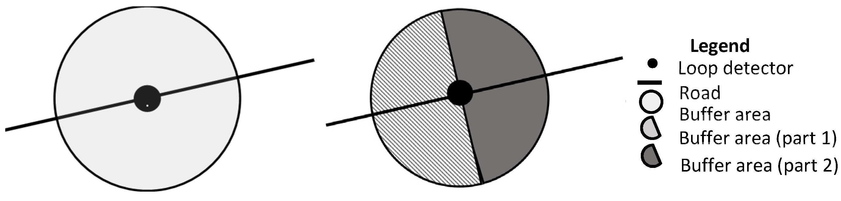
3.2. Buffer Area

This step aims to identify the extension of an area around the position of the selected traffic counters where the potentially spatiotemporal vehicle position is located. The individuation of this area is necessary for selecting the monitored road vehicles that will cross the traffic counter.

This is sub-divided into two steps: the extension and form, and the vehicle’s direction.

Extension and form. The buffer area may have different shapes (e.g., circle, ellipse, or rectangle). The choice of the shape depends on the road’s characteristics (the number of carriageways, lanes, lane width, etc.) and on the spatial position of the traffic counter in the road.

Vehicle direction. The buffer area is subdivided into two parts by an ideal line that is perpendicular to the longitudinal axis of the road. A numerical code is associated with each part; therefore, the buffer area is partitioned into “part 1” and “part 2” (Figure 2).

3.3. Vehicles’ Trajectories

This step aims to identify homogeneous trajectories for each monitored vehicle that potentially crosses the selected traffic counters.

This is subdivided into two steps: data sorting and trajectories.

Data sorting. The table containing the information collected in step 1 is re-arranged with a sorting procedure. Data are sorted using the numerical vehicle code and its temporal position.

Trajectories. A trajectory is an ordered sequence of spatiotemporal positions of a single vehicle. It is assumed that between two consecutive trajectories of the same vehicle, there is a fixed quantitative time lag (the threshold). The threshold’s value depends on the study’s aim.

3.4. Points, Vehicle, and Sub-Trajectory Selection

This step aims to select the spatiotemporal positions of the road vehicles that potentially cross each traffic counter.

This is subdivided into two steps: points and vehicles selection, and sub-trajectory selection.

Points and vehicle selection. By intersecting the available spatiotemporal positions of road vehicles (i), the buffer area and their parts, and the relative trajectories (k), a subset of positions is selected for each traffic counter.

Sub-trajectory selection. By considering the selected points, only the points belonging to the trajectories that have at least one point in the two parts of the buffer area are considered.

3.5. Couples of Spatial-Temporal Positions

This step aims to identify the couples of the points belonging to the two different parts of the buffer area for which the temporal interval is the minimum for each selected road vehicle and traffic counter.

This is subdivided into two steps: the segment and couple of the spatio-temporal points, and the spatio-temporal position selection.

The segment and couple of each spatio-temporal point. For each vehicle and selected sub-trajectory, it is possible to identify the segment that intersects with the diameter that divides the buffer area, in a direction perpendicular to the direction of traffic flow. The two extreme points of the segment represent a pair of consecutive space-time positions of the same vehicle (Figure 3). The two points are space-time positions of vehicle i along the sub-trajectory k; by ordering the records with respect to the column that contains the time, the first record represents the point belonging to part 1 of the buffer area, indicated as P1 (i, k); the other belongs to part 2 of the buffer area and is indicated as P2 (i, k).

Spatio-temporal position selection. Starting from positions P1 (i, k) and P2 (i, k), it is possible to select a predefined quantity of spatiotemporal positions belonging to the trajectory k:

• Before the time with respect to position P1 (i, k), belonging to the set P_before;
• After the time with respect to position P2 (i, k), belonging to the set P_after.

Figure 3 represents an example of the two sets, P_before and P_after, including five spatiotemporal positions before P1 (i, k) and after P2 (i, k).

3.6. Virtual Points

This step aims to identify the sub-trajectory and traffic counter for each selected road vehicle via the coupling of virtual points, representing the spatiotemporal positions of the two sets of real points before and after the traffic counter (P_before, P_after).

This is sub-divided in two steps: the virtual point before, and the virtual point after.

Virtual point before. Starting from the set P_before, the virtual point P1 ′(i, k) can be obtained by grouping the spatiotemporal positions located in the time before point P1 (i, k), assuming:

• The spatial position, a point that has spatial coordinates of:

  long_before = E[longitude of P_before]

  lat_before = E[latitude of P_before]
• The temporal position, a point that has temporal coordinates of:

  time_before = E[time of P_before]

Virtual point after. Starting from the set P_after, the virtual point P2′ (i, k) can be obtained by grouping the spatiotemporal positions located in the time before point P2 (i, k), assuming:

• The spatial position, a point that has spatial coordinates of:

  long_after = E[longitude of P_after]

  lat_after = E[latitude of P_after]
• The temporal position, a point that has temporal coordinates of:

  time_after = E[time of P_after]

3.7. Distances, Times, and Speeds

This step aims to identify the traffic counter, the sub-trajectory, and the obtained couple of virtual points for each selected road vehicle, with the following outputs.

• d (i, k), the spatial distance between the virtual points, calculated as:

  d (i, k) = [(long_after − long_before)² + (lat_after − lat_before)²]^0.5
• t(i,k), the temporal distance between the virtual points, calculated as:

  t (i, k) = time_after − time_before
• v (i, k), the speed of the vehicle i along the sub-trajectory k:

  v (i, k) = d (i, k)/t (i, k)

4. Method Experimentation with FCD

The proposed methodology has been experimentally tested in an area of the city of Santander, in the north of Spain (Figure 4). This area is the main access corridor, formed by two unidirectional three-lane parallel roads. This corridor presented the highest amount of average annual daily traffic in the city in 2019, channeling more than 30,000 vehicles per day and per direction. It also offers the main access to the rail and bus station, so it is one of the most frequently used roads by taxi services and it is equipped with an automatic traffic counter formed from magnetic loops (one per lane). This means that both GPS and loop detector data are available to be compared and combined. Specifically, the analyzed loops (IDs 1013 and 1008) are placed at the beginning of each road, downstream of the nearest traffic signal. The sections in which both automatic traffic counters are placed allow on-street parking in the left shoulder lane, and a taxi rank is also located at the end of the 1008 section (the left shoulder lane).

The method proposed in Section 3 is applied in this section in order to test the validity and the obtained results with respect to traditional and consolidated measurement systems. The integration between LDD and FCD has been experimentally established for loop 1013. The following part of this section is sub-divided into seven sub-sections that have a one-to-one correspondence with the seven sub-sections of Section 3.

4.1. Data Input

The input data refer to the space–time positions of the taxi fleet operating in the city of Santander.

The selected positions refer to the time interval between consecutive days from 28 March 2011 to 3 April 2011. The database assesses the space–time positions of the 194 monitored vehicles in the selected time interval. The spatial positions of each vehicle are available every 15 s, on average. The number of space–time positions amounts to 423,722.

A loop that was located in the road network of the city of Santander and was identified with the numerical code 1013 was also selected (Figure 4).

4.2. Buffer Area

A circular buffer area with a radius of 30 m was built around the spatial position of the selected traffic counter.

The buffer area was partitioned into two equal parts along a diameter perpendicular to the longitudinal axis of the road, according to the step described in Section 3.2 (“Vehicle direction”).

4.3. Vehicle Trajectories

The available space-time positions of each vehicle were sorted with respect to the time needed to identify the vehicles’ trajectories. Based on previous studies [33], the time threshold was set at 60 s. By applying this criterion for the entire time interval analyzed (3 days), 26,597 vehicles’ trajectories were obtained.

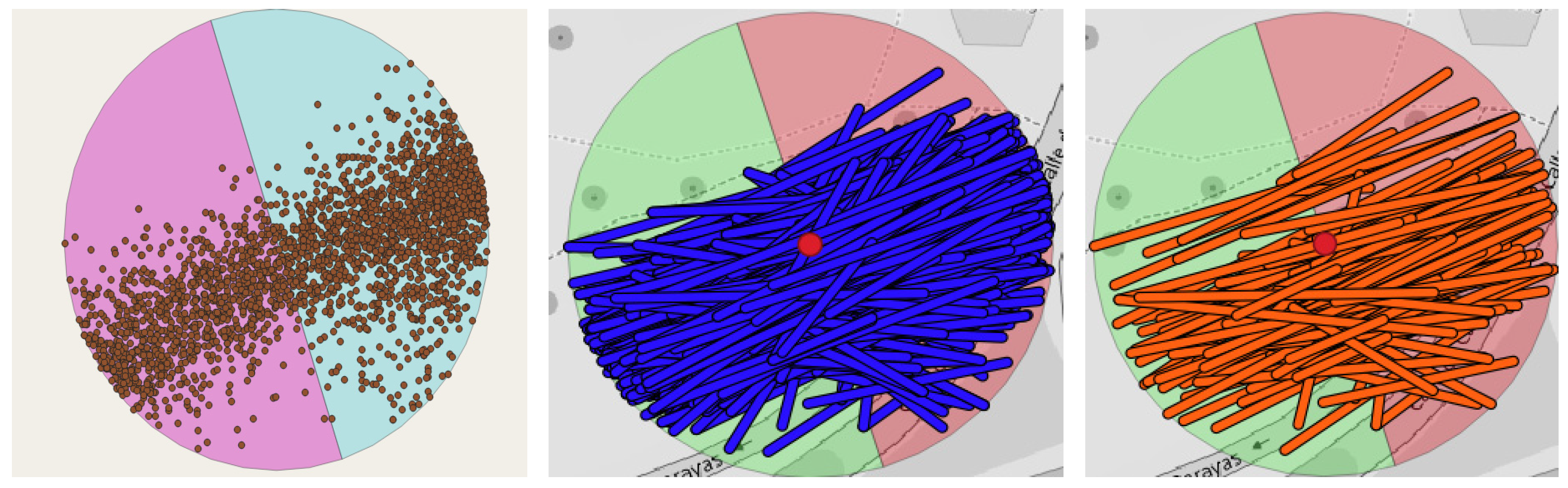
4.4. Point, Vehicle, and Sub-Trajectory Selection

The spatiotemporal positions belonging to the two parts into which the buffer area is sub-divided were selected. Figure 5 shows the positions in the case of traffic counter 1013. In particular, the picture on the left illustrates the selected spatiotemporal positions, the central picture shows the vehicles’ trajectories that cross the buffer area, and the picture on the right represents the sub-trajectories that have at least one point in each part of the buffer area.

Table 1. Vehicles, spatial-temporal positions, trajectories, and sub-trajectories.

	Traffic Counter 1013
Total Vehicles	193
Selected Vehicles	42
Spatiotemporal positions	1626
Total Trajectories	1297
Selected Sub-trajectories	48

gives a summary of the selected data relative to traffic counter 1013 (monitored vehicles, spatiotemporal positions, and trajectories); 42 vehicles and relative 48 sub-trajectories were selected.

4.5. Couples of Spatiotemporal Positions

The data synthetically described in Table 1 were used for identifying the coupled points. By considering the two positions of each couple, the five spatiotemporal positions before the first and those succeeding the second are considered.

4.6. Virtual Points

The spatiotemporal, real positions thus selected were processed to obtain the virtual points.

A couple of spatiotemporal vehicle positions were considered. The points P1 (i, k) and P2 (i, k) belong, respectively, to part 1 and part 2 of the buffer area around the analyzed traffic counter 1013.

Table 2. Example of real and virtual spatiotemporal positions on 29 March 2011.

	Positions in Space		Positions in Time
	(Longitude)	(Latitude)	(hh:mm:ss)
P1(1,1)	−3.82368	43.45279	07:29:19
Pbefore	−3.82259	43.45294	07:28:04
	−3.82261	43.45294	07:28:19
	−3.82347	43.45279	07:28:34
	−3.8239	43.45273	07:28:49
	−3.82392	43.45274	07:29:04
	−3.82368	43.45279	07:29:19
P1′ (1,1)	−3.82336	43.45282	07:28:41
P2 (1,1)	−3.82371	43.45276	07:29:34
Pafter	−3.82368	43.45279	07:29:19
	−3.82357	43.45280	07:29:49
	−3.82356	43.45278	07:35:19
	−3.82357	43.45279	07:35:34
	−3.82355	43.45280	07:35:49
	−3.82371	43.45276	07:29:34
P2′ (1, 1)	−3.8236	43.45279	07:32:34
	Spatial distance d (1, 1)	Temporal distance t (1, 1)	Speed
	(meters)	(minutes)	(km/h)
	890	3.8	14

P1 (1, 1) is the first real spatiotemporal point; P2 (1, 1) is the second real spatiotemporal point. P_before is the set of points before P1 (1, 1); P_after is the set of points after P2 (1, 1). P1′ (1, 1) is the first virtual spatiotemporal point; P2′ (1, 1) is the second virtual spatiotemporal point.

reports an example of the calculation of a virtual point for a couple of spatiotemporal positions on 29 March 2011. One vehicle (i = 1) and one sub-trajectory (k = 1) that cross the traffic counter are considered. The first and the second vehicle’s positions are indicated, respectively, as P1 (1,1) and P2 (1,1). The table reports the positions in space (longitude and latitude coordinates) and in time (in hours, hh, minutes, mm, and seconds, ss), before point P1 (1,1), belonging to the set P_before, and after P2 (1,1), belonging to the set P_after. The expected values of the coordinates in space (longitude and latitude) and in time (hh:mm:ss) represent the virtual spatiotemporal positions of the sets P_before, named P1′ (1,1), and P_after, named P2′ (1,1).

4.7. Distances, Times and Speeds

The virtual positions identified for each vehicle and sub-trajectory constitute the inputs for calculating first the spatial and temporal distances and then the speeds, by adopting the formulations described above. For instance, for the couple of virtual points given in Table 2 for vehicle 1 and sub-trajectory 1:

• The spatial distance d (1, 1) is equal to 890 m;
• The temporal distance t (1, 1) is equal to 228 s;
• The speed is equal to 3.9 m/s.

Figure 6 presents the distances and times for each selected vehicle that crosses traffic counter 1013. The slope of the segment connecting the origin and each point represents the estimated speed of each vehicle.

5. Method Validation with Loop Detectors

The proposed procedure allows the estimation of traffic flow variables, starting with the observation of:

• Flow and occupancy, by means of loop detectors;
• Speed, by means of GPS (or FCD) data.

It is worth noting that the observed occupancy and flow allow for estimating the three traditional traffic variables, such as flow, speed, and density, by assuming a certain hypothesis about the value of maximum density.

The following part of the paper is articulated as follows. Section 5.1 reports a theoretical specification that is present in the literature [18,33] on the FD. Section 5.2 presents the results of a statistical test, in order to verify the similarity of data provided by different sources. Section 5.3 presents the parameters estimated from loop-detector data, while Section 5.4 reports a comparison of the parameters estimated from loop-detector data and the FCD.

5.1. Drake Specification

Loop detectors provide flow, occupancy, and speed estimations for one minute. However, the speed values are biased, and they are considered not to be reliable by the traffic authority of the city of Santander.

GPS data, related to the same time period, were collected in order to compare and validate the proposed methodology. Thus, the first analysis focused on estimating the flow–occupancy relationships by means of different existing models, such as those of Greenshields, Drew, Underwood, Eddie, etc. Drake’s model (see [18,34]) was found to fit the observed data better.

According to Drake’s model [34], the estimated flow f_i in the time interval i can be obtained as follows:

f_i = k_i · v₀ · exp(−0.5 · (k_i/k*)²)

(4)

where:

• k_i is the density in time interval i;
• v₀ is the free-flow speed (parameter to be calibrated);
• k* is the density at capacity (parameter to be calibrated).

If the occupancy (o_i) is estimated, the density can be replaced, considering that:

k_i = o_i · k_L

(5)

with o_i, occupancy in the time interval i, and k_L, density–occupancy conversion factor (maximum density).

According to Equation (5), Equation (4) becomes:

f_i = o_i · k_L · v₀ · exp(−0.5 · (o_i · k_L/(o*· k_L))²)

(6)

f_i = o_i · a₀ · exp(−0.5 · (o_i/o*)²)

(7)

where o* is the occupancy at capacity.

a₀ = k_L · v₀, parameter to be calibrated

(8)

It is worth noting that the unit of measure of density is generally (veh/km) and that the occupancy is expressed as a decimal (with no dimension). Therefore, a₀ has the unit of measurement of [veh/h] and (o_i · a₀) has the unit of measurement of [100·veh/h].

According to the fundamental equation, v = f/k, the speed–occupancy relationship can be obtained from Equation (7) by considering the same parameters (a₀ and o*):

v_i = f_i/k_i = o_i·a₀·exp(−0.5 · (o_i/o*)²)/k_i = o_i · a₀ · exp(−0.5 · (o_i / o*)²)/(o_i · k_L) =
a₀ · exp(−0.5 · (o_i/o*)²)/k_L

(9)

v_i = v₀ · exp(−0.5 · (o_i/o*)²)

(10)

where v₀ = a₀/k_L is obtained from Equation (7).

5.2. Statistical Data Comparison

The paragraph reports the results of a statistical test conducted in order to verify the similarity of loop-detector data and GPS (FCD) data.

5.2.1. Speed Observation

The comparison was executed between the values of speed:

• Obtained from loop detector number 1013 (see Figure 7);
• Provided by GPS taxi data passing through the same loop.

The two speeds were estimated, considering different time aggregations of 15 min and 60 min. In both cases, the constant term is assumed to be equal to zero. Thus, two sets of data were extracted, obtaining 34 records (for 15 min) and 16 records (for 60 min), respectively. As shown in Figure 7, 60 min of aggregation presents a lower observed variance and slightly underestimates the speed, while 15 min of aggregation tends to overestimate the speeds and does not provide a good fit. When the speed–time profile is plotted (Figure 8), even when using a level of aggregation of 60 min, some time periods are not available since some GPS data were missing. However, in spite of this lack of data, a similar behavior can be observed in this case.

5.2.2. Test of the Hypothesis on Speed

Based on the comparison of different time periods of aggregation, 60 minutes of aggregation was used. The computation of speed averages and standard deviations for the two categories of speed data (loop detector and GPS) showed similar results of 51.84 km/h and 5.07 km/h for the loop data and 50.69 km/h and 5.47 km/h for the GPS data. A statistical test was executed to verify if the two couples of the values were equivalent. Student’s t-test was executed to verify the null hypothesis (H₀: ${\stackrel{-}{S}}_{\mathrm{loop}}-{\stackrel{-}{S}}_{\mathrm{GPS}}=0$) that both average values were the same. The null hypothesis was accepted because the values of the t-test fell inside the interval at the 0.05 percentile; there was no statistical evidence that the two estimated averages were different from one another (see

Table 3. Statistical tests for GPS speed: t-test for two samples, assuming unequal variances.

	Loop	GPS
Mean	51.8	50.6
Variance	25.67	31.86
Sample size	24	16
Hypothetical differences in means	0
t-test assuming different variances
Degree of freedom	27
t-test	0.70
P(T <= t) for one queue	0.24
t critical value (one queue)	1.70
P(T <= t) for two queues	0.49
t critical value (two queues)	2.05
Z test for two sample means
Z	1.54	1.65
P(Z <= z) one queue	0.06
z critical value (one queue)	1.64
z critical value (two queues)	0.12
z critical value (two queues)	1.96

).

5.3. Parameter Estimation with Loop Detector and FCD Data

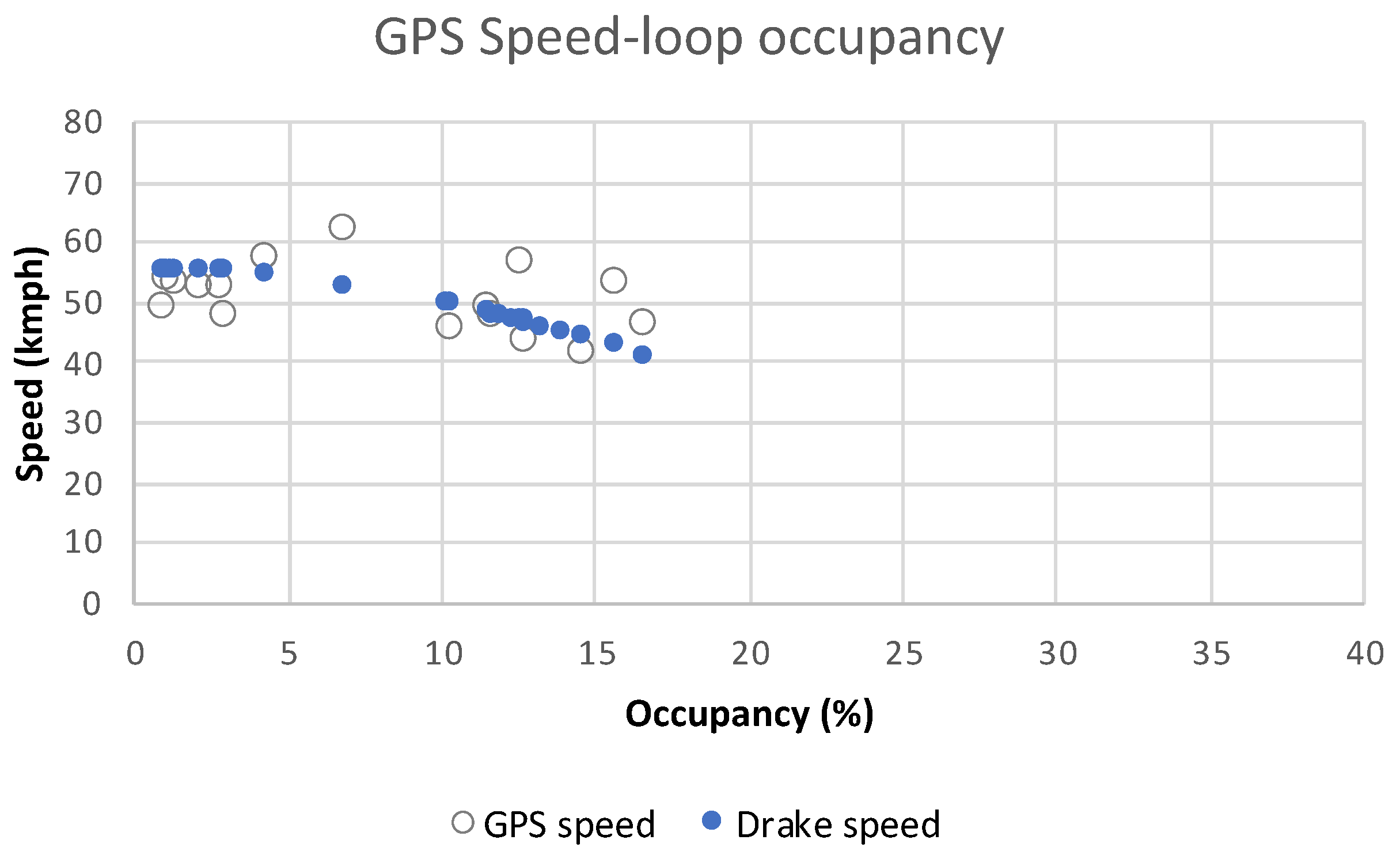
A first attempt was performed to calibrate a speed-occupancy diagram (Equation (10)) by means of speed values obtained from GPS and occupancy values obtained from the loop detector (a level of aggregation of 15 min). Because the available observed speed data lie inside the stable region of the diagram, the calibration of the two parameters, o* and v₀, of Equation (10) did not give statistically significant results.

Consequently, one parameter of the two parameters (o*) was exogenously assumed to be equal to the one estimated with loop detector data: o* = 21.7%. The result of the calibration of the single parameter, v₀, of the model (Equation (10)) is: v₀ = 55.6 [km/h]. The observed values vs. estimated values (with the Drake model) are plotted in Figure 9.

5.4. Parameters Estimation with Loop Detector Data

Flow and occupancy, observed with the loop detector, were initially used to calibrate the parameters a₀ and o* of Equation (8). The results of the calibration yielded a₀ = 200.8 [100·veh/h] and o* = 21.7 [%].

The observed values of flow and occupancy and the values estimated with Equation (8) are plotted in Figure 10.

According to Equation (8), the maximum density is: k_L = a₀/v₀ = 200.8 [100 veh/h]/55.6 [km/h] = 361.15 [veh/km], and the density at capacity value is: k_* = o* · k_l = 0.217 · 361.15 [veh/km] = 78.37 [veh/h].

The values thus calculated are acceptable, considering that the examined road has three lanes and it is situated in an urbanized area (with about one vehicle for each 8.3 m).

After estimation of the maximum density, occupancy measurements can be converted to densities by adopting Equation (5), and a flow-density relationship can be obtained by employing Drake’s model (Figure 11). The results of the comparison obtained with loop-detector data and GPS data are reported in

Table 4. Results obtained only with loop-detector data and by using both loop-detector and GPS data.

Flow and Occupancy from Loop Detector
Function	f = φ(o)
Drake model	fi = oi · a0 · exp(−0.5·(oi/o*)2)
Calibrated parameters *	a0 = 200.8 (100·veh/h) o* = 21.7%
GPS Speed and Occupancy from Loop Detector
Function	v = φ(o)
Drake model	vi = v0 · exp(−0.5·(oi/o*)2)
Calibrated parameters *	v0 = 55.6 km/h o* = 21.7% (estimation from loop)

* a₀ = k_L · v_0.

.

At the end of the calibration process, it is worth noting that the calibrated parameters are consistent with the traffic patterns observed in the examined road corridor.

6. Discussion and Conclusions

In this paper, consolidated research has been finalized to describe the traffic conditions on urban road links by means of FD, which requires the specification–calibration–validation of a flow-density function in relation to the geometric and functional characteristics of road infrastructures. FD is commonly associated with the links of the transport network and it has recently been extended to the transport network level, through the network macroscopic fundamental diagram (NMFD).

An FD at the link or network level is important for supporting the simulation, design, planning, and control of the transport system. Among the numerous applications of the FD, the calibrated flow-density curves (see the ones plotted in Figure 9 and Figure 11) may be used for building macroscopic traffic assignment models.

The traffic monitoring systems commonly used are based on loop-detector technology; however, FCD have become progressively more available for supporting traffic analysis. Today, it is necessary to integrate the two heterogeneous sources of information in order to increase our knowledge of mobility phenomena.

The research contribution of this paper concerns the proposal of a methodology for the extraction of speeds from FCD in the context of a specific link section and the calibration of FDs from FCD and LDD.

The methodology has been applied to a real case study in the city of Santander, in order to build an FD for a road link. The application consists of two steps.

• The execution of a statistical test was conducted to verify if the two sets of speed values obtained from FCD and from LDD are equivalent. Student’s t-test verified the null hypothesis that both average speed values referred to by the two sets are the same. In other words, there is no statistical evidence that the two estimated average speeds are different from one another.
• The calibration of a speed–occupancy diagram (Equation (10)) was achieved by means of speed values obtained from FCD and occupancy values obtained from LDD. The first calibrations presented in this paper are encouraging, supporting the thesis that FCD can be integrated with data obtained from loop detectors to build FDs.

The limits of this study concern the reduced quantity of available FCD, in terms of the lack of GPS data in some time periods and in terms of the availability of speed estimations being limited to the stable region of the speed–occupancy diagram. This last element led to a not statistically relevant estimation of the Drake model with the two parameters (related to occupancy and speed) and imposed an exogenous assumption of the parameter associated with occupancy.

Further advancements will be made in response to the availability of FCD (from GPS) and traffic data from an extended number of loop detectors. This availability will allow researchers to obtain more stable calibrations of an FD at the link level and to calibrate an NMFD at the network level.

References

- Zambrano-Martinez, J.L.; Calafate, C.T.; Soler, D.; Cano, J.C.; Manzoni, P. Modeling and characterization of traffic flows in urban environments. Sensors 2018, 18, 2020. [Google Scholar] [CrossRef]
- Johari, M.; Keyvan-Ekbatani, M.; Leclercq, L.; Ngoduy, D.; Mahmassani, H.S. Macroscopic network-level traffic models: Bridging fifty years of development toward the next era. Transp. Res. Part C Emerg. Technol. 2021, 131, 103334. [Google Scholar] [CrossRef]
- Croce, A.I.; Musolino, G.; Rindone, C.; Vitetta, A. Route and Path Choices of Freight Vehicles: A Case Study with Floating Car Data. Sustainability 2020, 12, 8557. [Google Scholar] [CrossRef]
- Croce, A.I.; Musolino, G.; Rindone, C.; Vitetta, A. Estimation of Travel Demand Models with Limited Information: Floating Car Data for Parameters’ Calibration. Sustainability 2021, 13, 8838. [Google Scholar] [CrossRef]
- Comi, A.; Rossolov, A.; Polimeni, A.; Nuzzolo, A. Private Car O-D Flow Estimation Based on Automated Vehicle Monitoring Data: Theoretical Issues and Empirical Evidence. Information 2021, 12, 493. [Google Scholar] [CrossRef]
- Battaglia, G.; Musolino, G.; Vitetta, A. Freight Demand Distribution in a Suburban Area: Calibration of an Acquisition Model with Floating Car Data. J. Adv. Transp. 2022, 2022, 1535090. [Google Scholar] [CrossRef]
- Cascetta, E. Transportation Systems Engineering: Theory and Methods; Springer: New York, NY, USA, 2001. [Google Scholar] [CrossRef]
- Torrieri, V.; Gattuso, D.; Musolino, G.; Vitetta, A. Density and conditioning characteristics of motorway vehicular traffic flow. In Proceedings of the International Conference on Applications of Advanced Technologies in Transportation Engineering, Capri, Italy, 27–30 June 1995; pp. 198–202. [Google Scholar]
- Iera, A.; Modafferi, A.; Musolino, G.; Vitetta, A. An experimental station for real-time traffic monitoring on a urban road. In Proceedings of the IEEE 5th International Conference on Intelligent Transportation Systems, Singapore, 3–6 September 2002; pp. 697–701. [Google Scholar] [CrossRef]
- Anda, C.; Erath, A.; Fourie, P.J. Transport modelling in the age of big data. Int. J. Urban Sci. 2017, 21, 19–42. [Google Scholar] [CrossRef]
- Nuzzolo, A.; Comi, A.; Papa, E.; Polimeni, A. Understanding Taxi Travel Demand Patterns Through Floating Car Data. In Data Analytics: Paving the Way to Sustainable Urban Mobility; Nathanail, E.G., Karakikes, I.D., Eds.; Springer International Publishing: Cham, Switzerland, 2019; Volume 879, pp. 445–452. [Google Scholar] [CrossRef]
- Nuzzolo, A.; Comi, A.; Polimeni, A. Exploring on-demand service use in large urban areas: The case of Rome. Arch. Transp. 2019, 50, 77–90. [Google Scholar] [CrossRef]
- Sananmongkhonchai, S.; Tangamchit, P.; Pongpaibool, P. Cell-based traffic estimation from multiple GPS-equipped cars. In Proceedings of the 2009 IEEE Region 10 Conference (TENCON 2009), Singapore, 23–26 January 2009; pp. 1–6. [Google Scholar]
- Godfrey, J. The mechanism of a road network. Traffic Eng. Control 1969, 11, 323–327. [Google Scholar]
- Herman, R.; Prigogine, I. A two-fluid approach to town traffic. Science 1979, 204, 148–151. [Google Scholar] [CrossRef]
- Mahmassani, H.; Williams, J.C.; Herman, R. Performance of urban traffic networks. In Proceedings of the 10th International Symposium on Transportation and Traffic Theory, Cambridge, MA, USA, 8–10 July 1987; pp. 1–20. [Google Scholar]
- Daganzo, C.F. Urban gridlock: Macroscopic modeling and mitigation approaches. Transp. Res. Part B Methodol. 2007, 41, 49–62. [Google Scholar] [CrossRef]
- Geroliminis, N.; Daganzo, C.F. Existence of urban-scale macroscopic fundamental diagrams: Some experimental findings. Transp. Res. Part B Methodol. 2008, 42, 759–770. [Google Scholar] [CrossRef]
- Alonso, B.; Pòrtilla, Á.I.; Musolino, G.; Rindone, C.; Vitetta, A. Network Fundamental Diagram (NFD) and traffic signal control: First empirical evidences from the city of Santander. Transp. Res. Procedia 2017, 27, 27–34. [Google Scholar] [CrossRef]
- Alonso, B.; Ibeas, Á.; Musolino, G.; Rindone, C.; Vitetta, A. Effects of traffic control regulation on Network Macroscopic Fundamental Diagram: A statistical analysis of real data. Transp. Res. Part A Policy Pract. 2019, 126, 136–151. [Google Scholar] [CrossRef]
- Aloi, A.; Alonso, B.; Benavente, J.; Cordera, R.; Echániz, E.; González, F.; Ladisa, C.; Lezama-Romanelli, R.; López-Parra, Á.; Mazzei, V.; et al. Effects of the COVID-19 Lockdown on Urban Mobility: Empirical Evidence from the City of Santander (Spain). Sustainability 2020, 12, 3870. [Google Scholar] [CrossRef]
- Yin, R.; Zheng, N.; Liu, Z. Estimating fundamental diagram for multi-modal signalized urban links with limited probe data. Phys. A Stat. Mech. Its Appl. 2022, 606, 128091. [Google Scholar] [CrossRef]
- Seo, T.; Kawasaki, Y.; Kusakabe, T.; Asakura, Y. Fundamental diagram estimation by using trajectories of probe vehicles. Transp. Res. Part B Methodol. 2019, 122, 40–56. [Google Scholar] [CrossRef]
- Kawasaki, Y.; Seo, T.; Kusakabe, T.; Asakura, Y. Fundamental diagram estimation using GPS trajectories of probe vehicles. In Proceedings of the 2017 IEEE 20th International Conference on Intelligent Transportation Systems (ITSC), Yokohama, Japan, 16–19 October 2017; pp. 1–6. [Google Scholar] [CrossRef]
- Deng, X.; Hu, Y.; Hu, Q. Fundamental Diagram Estimation Based on Random Probe Pairs on Sub-Segments. Promet-Traffic Transp. 2021, 22, 717–730. [Google Scholar] [CrossRef]
- Saffari, E.; Yildirimoglu, M.; Hickman, M. Data fusion for estimating Macroscopic Fundamental Diagram in large-scale urban networks. Transp. Res. Part C Emerg. Technol. 2022, 137, 103555. [Google Scholar] [CrossRef]
- Lu, S.; Jie, W.; van Zuylen, H.; Liu, X. Deriving the Macroscopic Fundamental Diagram for an urban area using counted flows and taxi GPS. In Proceedings of the 16th International IEEE Conference on Intelligent Transportation Systems (ITSC 2013), The Hague, The Netherlands, 6–9 October 2013; pp. 184–188. [Google Scholar] [CrossRef]
- Ji, Y.; Xu, M.; Li, J.; Van Zuylen, H.J. Determining the Macroscopic Fundamental Diagram from Mixed and Partial Traffic Data. Promet-Traffic Transp. 2018, 30, 267–279. [Google Scholar] [CrossRef]
- Ambühl, L.; Menendez, M. Data fusion algorithm for macroscopic fundamental diagram estimation. Transp. Res. Part C Emerg. Technol. 2016, 71, 184–197. [Google Scholar] [CrossRef]
- Tao, F.; Wu, J.; Lin, S.; Lv, Y.; Wang, Y.; Zhou, T. Revealing the Impact of COVID-19 on Urban Residential Travel Structure Based on Floating Car Trajectory Data: A Case Study of Nantong, China. ISPRS Int. J. Geo-Inf. 2023, 12, 55. [Google Scholar] [CrossRef]
- Wang, X.; Wu, Y.; Zhuang, D.; Sun, L. Low-Rank Hankel Tensor Completion for Traffic Speed Estimation. IEEE Trans. Intell. Transp. Syst. 2021, 24, 4862–4871. [Google Scholar] [CrossRef]
- Comi, A.; Polimeni, A. Estimating Path Choice Models through Floating Car Data. Forecasting 2022, 4, 525–537. [Google Scholar] [CrossRef]
- Croce, A.; Musolino, G.; Rindone, C.; Vitetta, A. Transport System Models and Big Data: Zoning and Graph Building with Traditional Surveys, FCD and GIS. ISPRS Int. J. Geo-Inf. 2019, 8, 187. [Google Scholar] [CrossRef]
- Drake, J.; Schofer, J.; May, A.D.J.R. A statistical analysis of speed-density hypotheses in vehicular traffic science. Highw. Res. Rec. 1966, 154, 53–87. [Google Scholar]
Figure 1.
Classification of monitoring systems for traffic data.
Figure 2.
Buffer area and its partition.
Figure 3.
Spatiotemporal position selection.
Figure 4.
Study area and localization of the studied junctions and the two parts of the buffer area around traffic counter 1013.
Figure 5.
Selected points (left), trajectories (center), and sub-trajectories (right).
Figure 6.
Graphical representation of the distances and times estimated with loop detector 1013.
Figure 7.
Loop-detector data vs. FCD speed data.
Figure 8.
Speed trends with loop-detector data and GPS data.
Figure 9.
Observed vs. estimated Drake values (speed–occupancy), with GPS and loop-detector data.
Figure 10.
Observed vs. estimated (with the Drake model) flow-occupancy values and the loop-detector data.
Figure 11.
Observed vs. theoretical Drake values (flow–density), considering GPS and loop detector data.