Quantifying Landscape-Scale Patterns of Temperate Forests over Time by Means of Neutral Simulation Models


Abstract
:1. Introduction
- (1)
- How did the spatial pattern of temperate forests change over time (1954–1981–2006)?
- (2)
- Is the spatial pattern change of these forests significantly different over time?
2. Methods
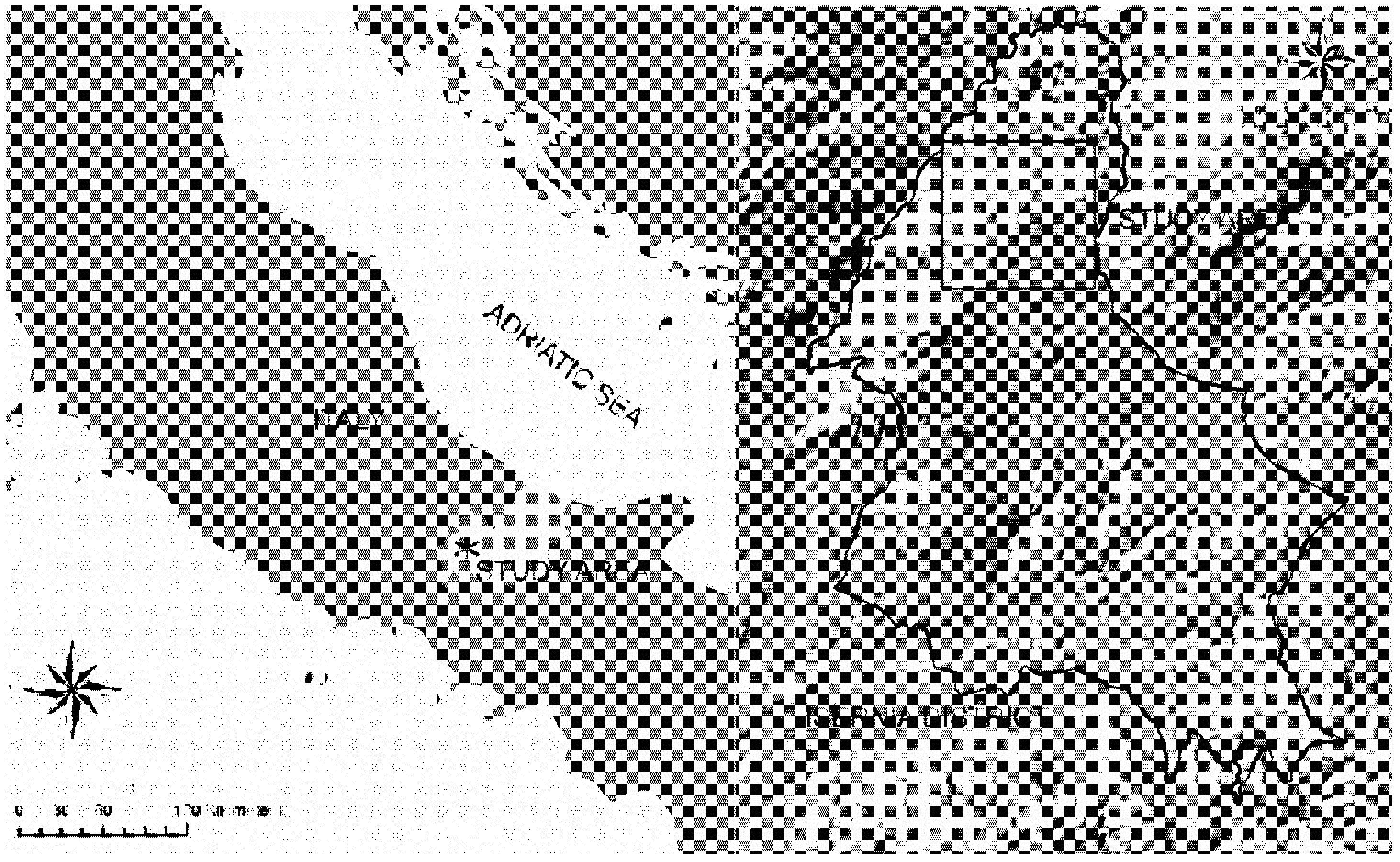
2.1. Study Area

2.2. Data Analysis
2.2.1. Data Preparation

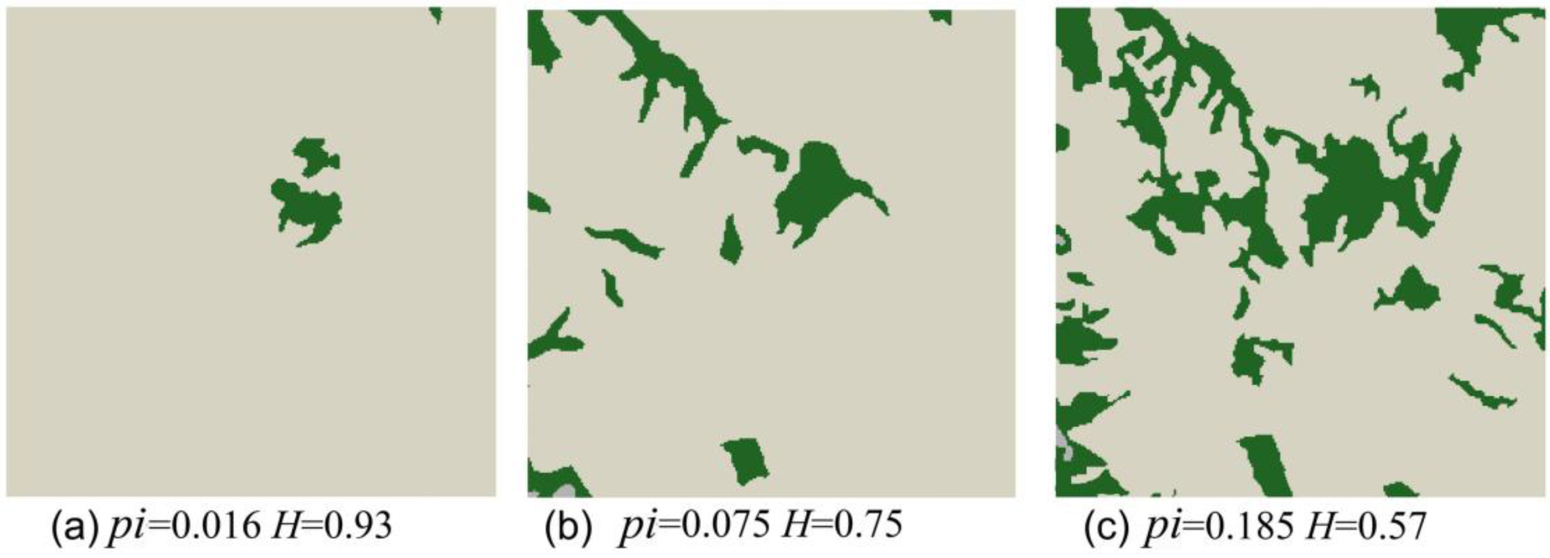
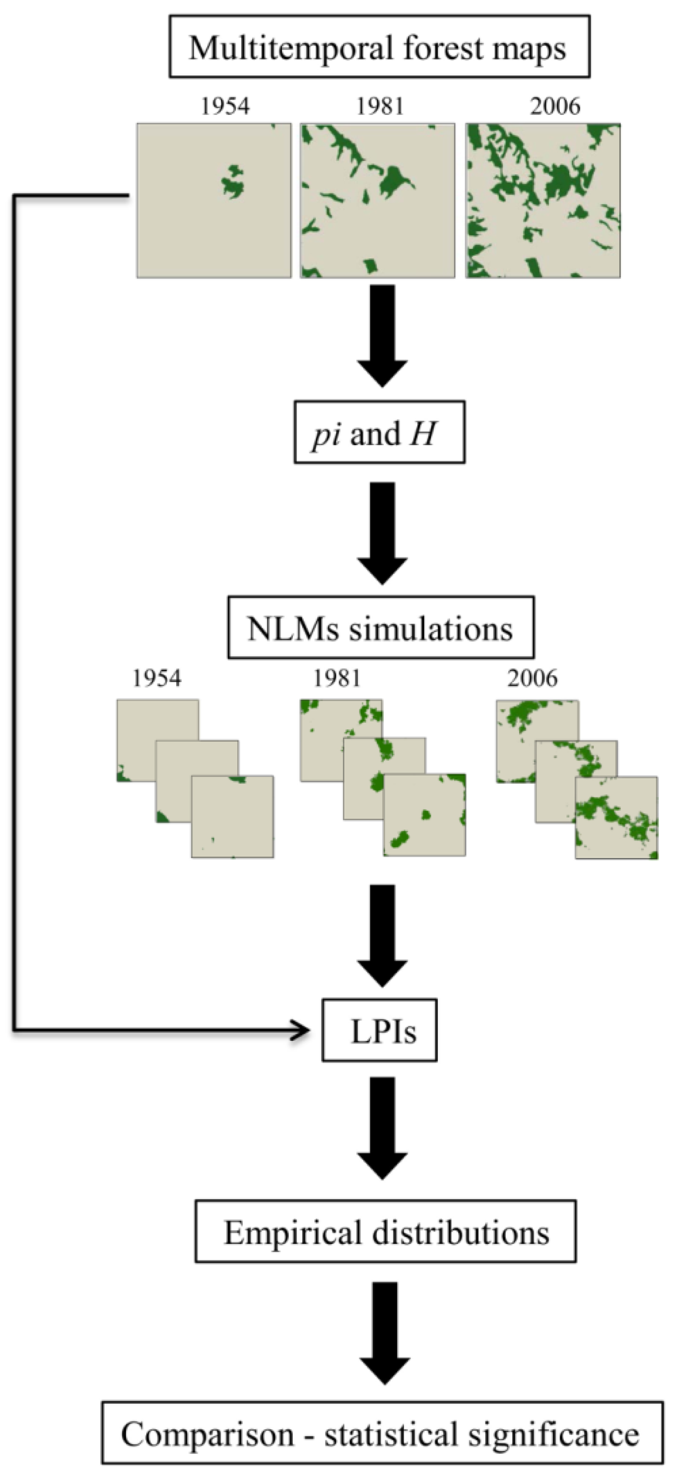
2.2.2. NLM
2.2.3. LPI Calculation
2.2.4. Comparing Observed and Simulated LPI
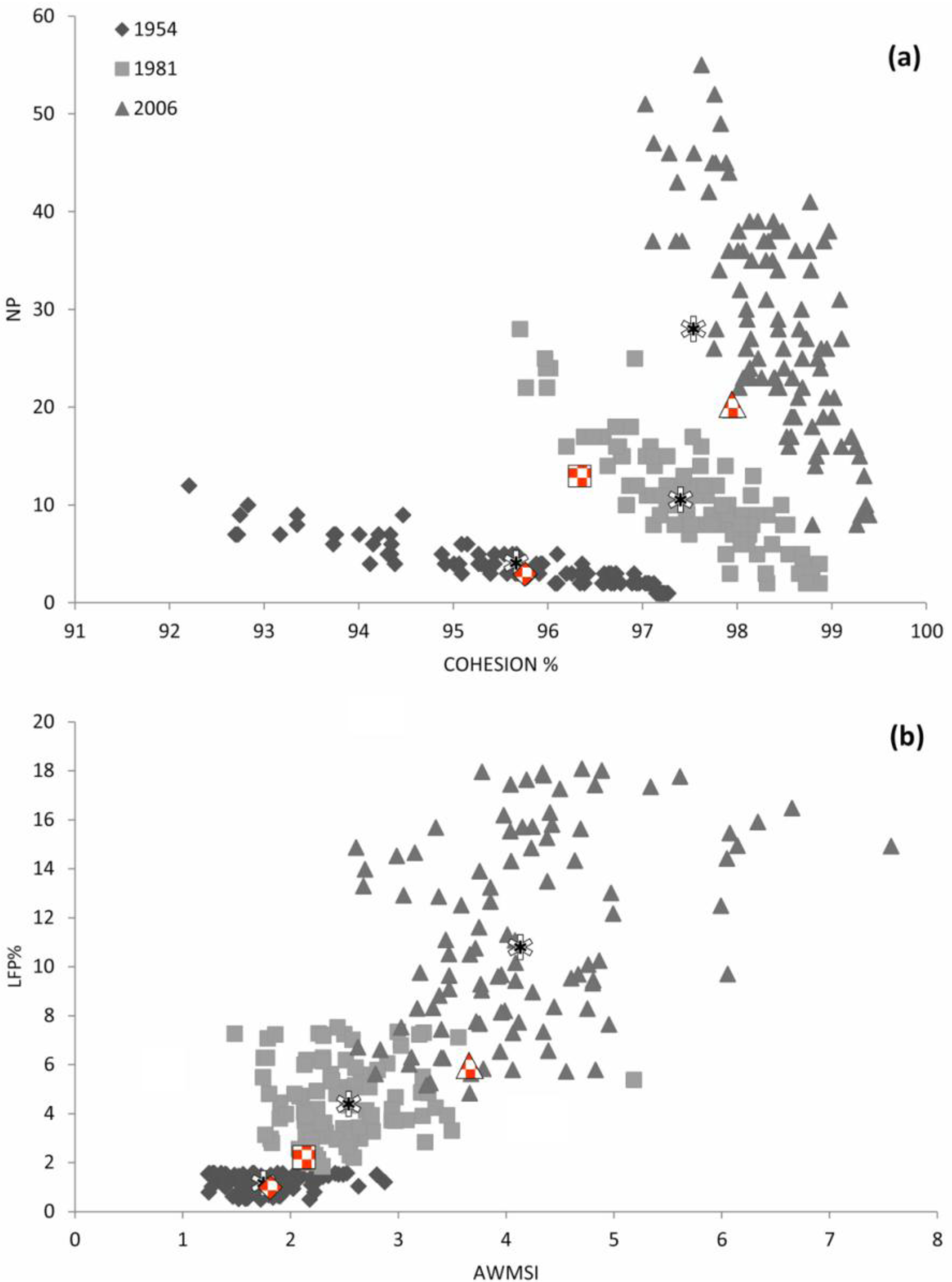
3. Results and Discussion
4. Conclusions
- (1)
- allows for modeling a reliable set of maps, which adequately describe the spatial pattern of forests through time and which can be directly compared with real landscapes [56];
- (2)
- generates a set of landscape replications, which account for the most relevant information;
- (3)
Acknowledgments
References and Notes
- Turner, M.G.; Gardner, R.H.; O’Neill, R.V. Landscape Ecology in Theory and Practice; Springer: New York, NY, USA, 2001. [Google Scholar]
- Dunn, C.P.; Sharpe, D.M.; Guntenspergen, G.R.; Stearns, F.; Yang, Z. Methods for Analyzing Temporal Changes in Landscape Pattern. In Quantitative Methods in Landscape Ecology; Turner, M.G., Gardner, R.H., Eds.; Springer-Verlag: New York, NY, USA, 1991; pp. 173–198. [Google Scholar]
- Franklin, J.F. Lessons from old-growth: Fueling controversy and providing direction. J. Forest 1993, 91, 10–13. [Google Scholar]
- Christensen, N.L.; Bartuska, A.M.; Brown, J.H.; Carpenter, S.; D’Antonio, C.; Francis, R.; Franklin, J.F.; MacMahon, J.A.; Noss, R.F.; Parsons, D.J.; et al. The report of the Ecological Society of America Committee on the scientific basis for ecosystem management. Ecol. Appl. 1996, 6, 665–691. [Google Scholar] [CrossRef]
- Kienast, F. Analysis of historic landscape patterns with a Geographical Information System—A methodological outline. Landscape Ecol. 1993, 8, 103–118. [Google Scholar] [CrossRef]
- Diekmann, M.; Eilertsen, O.; Fremstad, E.; Lawesson, J.E.; Aude, E. Beech forest communities in the Nordic countries—A multivariate analysis. Plant Ecol. 1999, 140, 203–220. [Google Scholar] [CrossRef]
- Axelsson, A.L.; Östlund, L. Retrospective gap analysis in a Swedish boreal forest landscape using historical data. Forest Ecol. Manage. 2001, 147, 109–122. [Google Scholar] [CrossRef]
- Rosati, L.; Fipaldini, M.; Marignani, M.; Blasi, C. Effects of fragmentation on vascular plant diversity in a Mediterranean forest archipelago. Plant. Biosyst. 2010, 144, 38–46. [Google Scholar] [CrossRef]
- MacDonald, D.; Crabtree, J.R.; Wiesinger, G.; Dax, T.; Stamou, N.; Fleury, P.; Gutierrez Lazpita, J.; Gibon, A. Agricultural abandonment in mountain areas of Europe: Environmental consequences and policy response. J. Environ. Manage. 2000, 59, 47–69. [Google Scholar] [CrossRef]
- Antrop, M. Landscape change and the urbanization process in Europe. Landscape Urban Plan. 2004, 67, 9–26. [Google Scholar] [CrossRef]
- Rudel, T.K.; Coomes, O.T.; Moran, E.; Achard, F.; Angelsen, A.; Xu, J.; Lambin, E. Forest transitions: Towards a global understanding of land use change. Global Environ. Change. 2005, 15, 23–31. [Google Scholar] [CrossRef]
- Carranza, M.L.; Acosta, A.; Ricotta, C. Analyzing landscape diversity in time: The use of Rènyi’s generalized entropy function. Ecol. Indic. 2007, 7, 505–510. [Google Scholar] [CrossRef]
- Van Gils, H.; Batsukh, O.; Rossiter, D.; Munthali, W.; Liberatoscioli, E. Forecasting the pattern and pace of Fagus forest expansion in Majella National Park, Italy. Appl. Veg. Sci. 2008, 11, 539–546. [Google Scholar] [CrossRef]
- Bracchetti, L.; Carotenuto, L.; Catorci, A. Land-cover changes in a remote area of central Apennines (Italy) and management directions. Landscape Urban Plan. 2012, 104, 157–170. [Google Scholar] [CrossRef]
- Kramer, R.A.; Richter, D.D.; Pattanayak, S.; Sharma, N.P. Ecological and economic analysis of watershed protection in Eastern Madagascar. J. Environ. Manage. 1997, 49, 277–295. [Google Scholar] [CrossRef]
- Houghton, R.A.; Skole, D.L.; Nobre, C.A.; Hackler, J.L.; Lawrence, K.T.; Chomentowski, W.H. Annual fluxes of carbon from deforestation and regrowth in the Brazilian Amazon. Nature 2000, 403, 301–304. [Google Scholar]
- Nabuurs, G.J.; Schelhaas, M.-J.; Mohren, G.M.J.; Field, C.B. Temporal evolution of the European forest sector carbon sink from 1950 to 1999. Glob. Change Biol. 2003, 9, 152–160. [Google Scholar] [CrossRef]
- Fahrig, L. Effects of habitat fragmentation on biodiversity. Annu. Rev. Ecol. Evol. S. 2003, 34, 487–515. [Google Scholar] [CrossRef]
- Estreguil, C.; Mouton, C. Measuring and Reporting on Forest Landscape Pattern, Fragmentation and Connectivity in Europe: Methods and Indicators; EUR 23841 EN; European Commision Joint Research Center, Office for Official Publications of the European Communities: Luxembourg, 2009. [Google Scholar]
- O’Neill, R.V.; Krummel, J.R.; Gardner, R.H.; Sugihara, G.; Jackson, B.; de Angelis, D.L.; Milne, B.T.; Turner, M.G.; Zygmunt, B.; Christensen, S.W.; et al. Indices of landscape pattern. Landscape Ecol. 1988, 1, 153–162. [Google Scholar] [CrossRef]
- Turner, M.G. Landscape ecology: The effect of pattern on process. Annu. Rev. Ecol. Evol. S. 1989, 20, 171–197. [Google Scholar]
- Ritters, K.H.; O’Neill, R.V.; Hunsaker, C.T.; Wickham, J.D.; Yankee, D.H.; Timmins, S.P.; Jones, B.K.; Jackson, B.L. A factor analysis of landscape pattern and structure metrics. Landscape Ecol. 1995, 10, 23–39. [Google Scholar] [CrossRef]
- Hessburg, P.F.; Smith, B.G.; Salter, R.B. Detecting change in forest spatial patterns from reference conditions. Ecol. Appl. 1999, 9, 1232–1252. [Google Scholar] [CrossRef]
- Frohn, R.; Hao, Y. Landscape metric performance in analyzing two decades of deforestation in the Amazon Basin of Rondonia, Brazil. Remote Sens. Environ. 2006, 100, 237–251. [Google Scholar] [CrossRef]
- Turner, M.G.; Person, S.M.; Bolstad, P.; Wear, D.N. Effects of land-cover change on spatial pattern of forest communities in the Southern Appalachian Mountains (USA). Landscape Ecol. 2003, 18, 449–464. [Google Scholar] [CrossRef]
- Gergel, S.E. New Direction in Landscape Pattern Analysis and Linkages with Remote Sensing. In Understanding Forest Disturbance and Spatial Pattern: Remote Sensing and GIS Approaches; Wulder, M.A., Franklin, S.E., Eds.; Taylor and Francis: Boca Raton, FL, USA, 2007; pp. 173–208. [Google Scholar]
- Cullinan, V.I; Thomas, M. A comparison of quantitative methods for examining landscape pattern and scale. Landscape Ecol. 1992, 7, 211–227. [Google Scholar] [CrossRef]
- Gustafson, E.J.; Parker, G.R. Relationships between landcover proportion and indexes of landscape spatial pattern. Landscape Ecol. 1992, 7, 101–110. [Google Scholar] [CrossRef]
- Wickham, J.D.; Riitters, K.H. Sensitivity of landscape metrix to pixel size. Int. J. Remote Sens. 1995, 16, 3585–3594. [Google Scholar] [CrossRef]
- Rocchini, D. Resolution problems in calculating landscape metrics. J.Spat. Sci. 2005, 50, 25–36. [Google Scholar] [CrossRef]
- Saura, S.; Martínez-Millán, J. Sensitivity of lanscape pattern metrics to map spatial extent. Photogramm. Eng. Remote Sensing 2001, 67, 1027–1036. [Google Scholar]
- Wickham, J.D.; O’Neill, R.V.; Riitters, K.H.; Wade, T.G.; Jones, K.B. Sensitivity of selected landscape pattern metrics to land-cover misclassification and differences in land-cover caomposition. Photogramm. Eng. Remote Sensing 1997, 63, 397–402. [Google Scholar]
- Long, J.A.; Nelson, T.A.; Wulder, M.A. Characterizing forest fragmentation: Distinguishing change in composition from configuration. Appl. Geogr. 2010, 30, 426–435. [Google Scholar] [CrossRef]
- Boots, B.; Csillag, F. Categorical maps, comparisons, and confidence. J. Geogr. Syst. 2006, 8, 109–118. [Google Scholar] [CrossRef]
- Remmel, T.K.; Csillag, F. When are two landscape pattern indices significantly different? J. Geogr. Syst. 2003, 5, 331–351. [Google Scholar] [CrossRef]
- Csillag, F.; Boots, B. A framework for statistical inferential decisions in spatial pattern analysis. Can. Geogr. 2005, 49, 172–179. [Google Scholar] [CrossRef]
- Keitt, T.H. Spectral representation of neutral landscapes. Landscape Ecol. 2000, 15, 479–493. [Google Scholar] [CrossRef]
- Pearson, S.M.; Gardner, R.H. Neutral Models: Useful Tools for Understanding Landscape Patterns. In Wildlife and Landscape Ecology: Effects of Pattern and Scale; Bisonette, J.A., Ed.; Springer: New York, NY, USA, 1997; pp. 215–230. [Google Scholar]
- Gardner, R.H.; Milne, B.T.; Turner, M.G.; O’Neill, R.V. Neutral models for the analysis of broad-scale landscape pattern. Landscape Ecol. 1987, 1, 19–28. [Google Scholar] [CrossRef]
- Milne, B.T. Spatial aggregation and neutral models in fractal landscapes. Am. Naturalist 1992, 139, 32–57. [Google Scholar]
- O’Neill, R.V.; Gardner, R.H.; Turner, M.G. A hierarchical neutral model for landscape analysis. Landscape Ecol. 1992, 7, 55–61. [Google Scholar] [CrossRef]
- With, K.A.; King, A.W. The use and misuse of neutral landscape models in ecology. Oikos 1997, 79, 219–229. [Google Scholar] [CrossRef]
- Stauffer, D.; Aharony, A. Introduction to Percolation Theory, 2nd ed; CRC Press Inc.: London, UK, 1994. [Google Scholar]
- Mandelbrot, B.B. The Fractal Geometry of Nature; W. H. Freeman and Company Ltd.: New York, NY, USA, 1982. [Google Scholar]
- Saupe, D. Algorithms for Random Fractals. In The Science of Fractal Images; Peitgen, H.O., Saupe, D., Barnsley, M.F., Eds.; Springer-Verlag: New York, NY, USA, 1988; pp. 71–113. [Google Scholar]
- With, K.A.; Gardner, R.H.; Turner, M.G. Landscape connectivity and population distributions in heterogeneous environments. Oikos 1997, 78, 151–169. [Google Scholar] [CrossRef]
- With, K.A.; King, A.W. Dispersal success on fractal landscapes: A consequence of lacunarity thresholds. Landscape Ecol. 1999, 14, 73–82. [Google Scholar] [CrossRef]
- With, K.A.; Cadaret, S.J.; Davis, C. Movement responses to patch structure in experimental fracta landscapes. Ecology 1999, 80, 1340–1353. [Google Scholar] [CrossRef]
- With, K.A.; King, A.W. The effect of landscape structure on community self-organization and critical biodiversity. Ecol. Model. 2004, 179, 349–366. [Google Scholar] [CrossRef]
- Palmer, M.W. The coexistence of species in fractal landscapes. Am. Naturalist 1992, 139, 375–397. [Google Scholar]
- Moloney, K.A.; Levin, S.A. The effects of disturbance architecture on landscape-level population dynamics. Ecology 1996, 77, 375–394. [Google Scholar] [CrossRef]
- Zurlini, G.; Riitters, K.H.; Zaccarelli, N.; Petrosillo, I. Patterns of disturbances at multiple scales in real and simulated landscapes. Landscape Ecol. 2007, 22, 705–721. [Google Scholar] [CrossRef]
- Zaccarelli, N.; Petrosillo, I.; Zurlini, G.; Riitters, K.H. Source/Sink Patterns of Disturbance and Cross-Scale Mismatches in a Panarchy of Social-Ecological Landscapes. Available online: http://www.ecologyandsociety.org/vol13/iss1/art26/ (accessed on 5 February 2013).
- Ricotta, C.; Carranza, M.L.; Avena, G.; Blasi, C. Are potential natural vegetation maps a meaningful alternative to neutral landscape models? Appl. Veg. Sci. 2002, 5, 271–275. [Google Scholar] [CrossRef]
- Hargrove, W.; Hoffman, F.M.; Schwartz, P.M. A Fractal Landscape Realizer for Generating Synthetic Maps. Available online: http://www.ecologyandsociety.org/vol6/iss1/art2/ (accessed on 25 September 2012).
- Neel, M.C.; McGarigal, K.; Cushman, S.A. Behavior of class-level landscape metrics across gradients of class aggregation and area. Landscape Ecol. 2004, 19, 435–455. [Google Scholar] [CrossRef]
- Gardner, R.H. RULE: A Program for the Generation of Random Maps and the Analysis of Spatial Patterns. In Landscape Ecological Analysis: Issues and Applications; Klopatek, J.M., Gardner, R.H., Eds.; Springer-Verlag: New York, NY, USA, 1999; pp. 280–303. [Google Scholar]
- Acosta, A.; Carranza, M.L.; Giancola, M. Landscape change and ecosystem classification in a municipal district of a small city (Isernia, Central Italy). Environ. Monit. Assess. 2005, 108, 323–335. [Google Scholar] [CrossRef]
- Li, H.; Reynolds, J.F. A new contagion index to quantify spatial patterns of landscapes. Landscape Ecol. 1993, 8, 155–162. [Google Scholar] [CrossRef]
- With, K.A. The applications of neutral landscape models in conservation biology. Conserv. Biol. 1997, 11, 1069–1080. [Google Scholar]
- Saura, S. Effects of minimum mapping unit on land cover data spatial configuration and composition. Int. J. Remote Sens. 2002, 23, 4853–4880. [Google Scholar] [CrossRef]
- McGarigal, K.; Cushman, S.A.; Ene, E. FRAGSTATS V. 4. Spatial Pattern Analysis Program for Categorical and Continuous Maps. Available online: http://www.umass.edu/landeco/research/fragstats/fragstats.html (accessed on 20 September 2012).
- Schindler, S.; Poirazidis, K.; Wrbka, T. Towards a core set of landscape metrics for biodiversity assessments: A case study from Dadia National Park, Greece. Ecol. Indic. 2008, 8, 502–514. [Google Scholar] [CrossRef]
- Haines-Young, R.; Chopping, M. Quantifying landscape structure: A review of landscape indices and their application to forested landscapes. Prog. Phys. Geogr. 1996, 20, 418–445. [Google Scholar] [CrossRef]
- Saura, S.; Martínez-Millán, J. Landscape patterns simulation with a modified random cluster methods. Landscape Ecol. 2000, 15, 661–678. [Google Scholar] [CrossRef]
- Armenteras, D.; Gast, F.; Villareal, H. Andean forest fargmentation and the representativeness of protected natural areas in the esatern Andes, Colombia. Biol. Conserv. 2003, 113, 245–256. [Google Scholar] [CrossRef]
- Batistella, M.; Robeson, S.; Moran, E.F. Settlement design, forest fragmentation, and landscape change in Rondonia, Amazonia. Photogramm. Eng. Remote Sensing 2003, 69, 805–812. [Google Scholar]
- Rocchini, D.; Perry, G.L.W.; Salerno, M.; Maccherini, S.; Chiarucci, A. Landscape change and the dynamics of open formations in a natural reserve. Landscape Urban Plan. 2006, 77, 167–177. [Google Scholar] [CrossRef]
- Sitzia, T.; Semenzato, P.; Trentanovi, G. Natural reforestation is changing spatial patterns of rural mountain and hill landscapes: A global overview. Forest Ecol. Manage. 2010, 259, 1354–1362. [Google Scholar] [CrossRef]
- Forman, R.T.T. Some general principles of landscape and regional ecology. Landscape Ecol. 1995, 10, 133–142. [Google Scholar] [CrossRef]
- Forman, R.T.T.; Godron, M. Landscape Ecology; John Wiley & Sons: New York, NY, USA, 1986. [Google Scholar]
- Fitzsimmons, M. Effects of deforestation and reforestation on landscape spatial structure in boreal Saskatchewan, Canada. Forest Ecol. Manage. 2003, 174, 577–592. [Google Scholar] [CrossRef]
- Southworth, J.; Nagendra, H.; Carlson, L.A.; Tucker, C. Assessing the impact of Celaque National Park on forest fragmentation in western Honduras. Appl. Geogr. 2004, 24, 303–322. [Google Scholar] [CrossRef]
- McGarigal, K.; Marks, B. FRAGSTATS, Spatial Pattern Analysis Program for Quantifying Landscape Structure; PNW-GTR-351; US Department of Agriculture, Forest Service, Pacific Northwest Research Station: Portland, OR, USA, 1995. [Google Scholar]
- Schumaker, N.H. Using landscape indices to predict habitat connectivity. Ecology 1996, 77, 1210–1225. [Google Scholar] [CrossRef]
- Opdam, P.; Verboom, J.; Pouwels, R. Landscape cohesion: an index for the conservation potential of landscapes for biodiversity. Landscape Ecol. 2003, 18, 113–126. [Google Scholar] [CrossRef]
- Fortin, M.-J.; Boots, B.; Csillag, F. On the role of spatial stochastic models in understanding landscape indices in ecology. Oikos 2003, 102, 203–212. [Google Scholar] [CrossRef]
- Torta, G. Consequences of Rural Abandonment in a Northern Apennines Landscape (Tuscany, Italy). In Recent Dynamics of the Mediterranean Vegetation and Landscape; Mazzoleni, S., di Martino, P., Strumia, S., Buonanno, M., Bellelli, M., Eds.; John Wiley & Sons, Ltd.: Chichester, UK, 2005; pp. 157–165. [Google Scholar]
- Mazzoleni, S.; Martino, P.D.; Strumia, S.; Buonanno, M.; Bellelli, M. Recent Changes of Coastal and Sub-Mountain Vegetation Landscape in Campania and Molise Regions in Southern Italy. In Recent Dynamics of the Mediterranean Vegetation and Landscape; Mazzoleni, S., di Pasquale, G., Mulligan, M., di Martino, P., Rego, F., Eds.; John Wiley & Sons, Ltd.: Chichester, UK, 2005; pp. 143–155. [Google Scholar]
- Globevnik, L.; Kaligarič, M.; Sovinc, A. Forest Cover Progression, Land-Use and Socio-Economic Changes on the Edge of the Mediterranean. In Recent Dynamics of the Mediterranean Vegetation and Landscape; Mazzoleni, S., di Pasquale, G., Mulligan, M., di Martino, P., Rego, F., Eds.; John Wiley & Sons, Ltd.: Chichester, UK, 2005; pp. 249–256. [Google Scholar]
- Lasanta-Martínez, T.; Vicente-Serrano, S.M.; Cuadrat-Prats, J.M. Mountain Mediterranean landscape evolution caused by the abandonment of traditional primary activities: A study of the Spanish Central Pyrenees. Appl. Geogr. 2005, 25, 47–65. [Google Scholar] [CrossRef]
- Guirado, M.; Pino, J.; Rodà, F.; Basnou, C. Quercus and Pinus cover are determined by landscape structure and dynamics in peri-urban Mediterranean forest patches. Plant Ecol. 2007, 194, 109–119. [Google Scholar] [CrossRef]
- Vos, W.; Stortelder, A. Vanishing Tuscan Landscapes: Landscape Ecology of a Submediterranean-Montane Area (Solano Basin, Tuscany, Italy); Pudoc Scientific Publishers: Wageningen, NL, USA, 1992. [Google Scholar]
- Myster, R.W.; Malahy, M.P. Is there a middle way between permanent plots and chronosequences? Can. J. Forest Res. 2008, 38, 3133–3138. [Google Scholar] [CrossRef]
- Myster, R.W.; Pickett, S.T.A. A comparison of rate of succession over 18 Yr in 10 contrasting old fields. Ecology 1994, 75, 387–392. [Google Scholar] [CrossRef]
- Pueyo, Y.; Beguería, S. Modelling the rate of secondary succession after farmland abandonment in a Mediterranean mountain area. Landscape Urban Plan. 2007, 83, 245–254. [Google Scholar] [CrossRef]
- Li, X.; He, H.S.; Wang, X.; Bu, R.; Hu, Y.; Chang, Y. Evaluating the effectiveness of neutral landscape models to represent a real landscape. Landscape Urban Plan. 2004, 69, 137–148. [Google Scholar] [CrossRef]
- Tatoni, T.; Médail, F.; Roche, P.; Barbero, M. The Impact of Changes in Land Use on Ecological Patterns in Provence (Mediterranean France). In Recent Dynamics of the Mediterranean Vegetation and Landscape; Mazzoleni, S., di Pasquale, G., Mulligan, M., di Martino, P., Rego, F., Eds.; John Wiley & Sons, Ltd.: Chichester, UK, 2005; pp. 105–120. [Google Scholar]
- Coelho-Silva, J.L.; Castro Rego, F.; Castelbranco Silveira, S.; Cardoso Gonçalves, C.P.; Machado, C.A. Rural Changes and Landscape in Serra da Malcata, Central East of Portugal. In Recent Dynamics of the Mediterranean Vegetation and Landscape; Mazzoleni, S., di Pasquale, G., Mulligan, M., di Martino, P., Rego, F., Eds.; John Wiley & Sons, Ltd.: Chichester, UK, 2005; pp. 189–200. [Google Scholar]
- Geri, F.; Rocchini, D.; Chiarucci, A. Landscape metrics and topographical determinants of large-scale forest dynamics in a Mediterranean landscape. Landscape Urban Plan. 2010, 95, 46–53. [Google Scholar] [CrossRef]
- Bertacchi, A.; Onnis, A. Changes in the Forested Agricultural Landscape of the Pisan Hills (Tuscany, Italy). In Recent Dynamics of the Mediterranean Vegetation and Landscape; Mazzoleni, S., di Pasquale, G., Mulligan, M., di Martino, P., Rego, F., Eds.; John Wiley & Sons, Ltd.: Chichester, UK, 2005; pp. 167–178. [Google Scholar]
- Zerbe, S. Potential natural vegetation: Validity and applicability in landscape planning and nature conservation. Appl. Veg. Sci. 1998, 1, 165–172. [Google Scholar] [CrossRef]
- Kolb, A.; Diekmann, M. Effects of life-history traits on responses of plant species to forest fragmentation. Conserv. Biol. 2005, 19, 929–938. [Google Scholar] [CrossRef]
- Carranza, M.L.; Frate, L.; Paura, B. Structure, ecology and plant richness patterns in fragmented beech forests. Plant Ecol. Divers. 2012, 5, 541–551. [Google Scholar] [CrossRef]
- Mortelliti, A.; Amori, G.; Capizzi, D.; Cervone, C.; Fagiani, S.; Pollini, B.; Boitani, L. Independent effects of habitat loss, habitat fragmentation and structural connectivity on the distribution of two arboreal rodents. J. Appl. Ecol. 2011, 48, 153–162. [Google Scholar] [CrossRef]
- Silver, W.L.; Ostertag, R.; Lugo, A.E. The potential for carbon sequestration through reforestation of abandoned tropical agricultural and pasture lands. Restor. Ecol. 2000, 8, 394–407. [Google Scholar] [CrossRef]
- Van Dijk, A.I.J.M.; Hairsine, P.B.; Arancibia, J.P.; Dowling, T.I. Reforestation, water availability and stream salinity: A multi-scale analysis in the Murray-Darling Basin, Australia. Forest Ecol. Manage. 2007, 251, 94–109. [Google Scholar] [CrossRef]
- Bathurst, J.C.; Bovolo, C.I.; Cisneros, F. Modelling the effect of forest cover on shallow landslides at the river basin scale. Ecol. Eng. 2010, 36, 317–327. [Google Scholar] [CrossRef] [Green Version]
- Gellrich, M.; Baur, P.; Koch, B.; Zimmermann, N.E. Agricultural land abandonment and natural forest re-growth in the Swiss mountains: A spatially explicit economic analysis. Agr. Ecosyst. Environ. 2007, 118, 93–108. [Google Scholar] [CrossRef]
- Frank, S.; Fürst, C.; Koschke, L.; Makeschin, F. A contribution towards a transfer of the ecosystem service concept to landscape planning using landscape metrics. Ecol. Indic. 2012, 21, 30–38. [Google Scholar] [CrossRef]
- Blondel, J.; Aronson, J. Biology and Wildlife of the Mediterranean Region; Oxford University Press: Oxford, UK, 1999. [Google Scholar]
- Wainwright, J.; Thornes, J.B. Environmental Issues in the Mediterranean Processes and Perspectives from the Past and Present; Rutledge: London, UK, 2004. [Google Scholar]
- Zurlini, G.; Petrosillo, I.; Jones, K.B.; Zaccarelli, N. Highlighting order and disorder in social-ecological landscapes to foster adaptive capacity and sustainability. Landscape Ecol. 2012. [Google Scholar] [CrossRef]
© 2013 by the authors; licensee MDPI, Basel, Switzerland. This article is an open access article distributed under the terms and conditions of the Creative Commons Attribution license (http://creativecommons.org/licenses/by/3.0/).
Share and Cite
Frate, L.; Carranza, M.L. Quantifying Landscape-Scale Patterns of Temperate Forests over Time by Means of Neutral Simulation Models. ISPRS Int. J. Geo-Inf. 2013, 2, 94-109. https://doi.org/10.3390/ijgi2010094
Frate L, Carranza ML. Quantifying Landscape-Scale Patterns of Temperate Forests over Time by Means of Neutral Simulation Models. ISPRS International Journal of Geo-Information. 2013; 2(1):94-109. https://doi.org/10.3390/ijgi2010094
Chicago/Turabian StyleFrate, Ludovico, and Maria Laura Carranza. 2013. "Quantifying Landscape-Scale Patterns of Temperate Forests over Time by Means of Neutral Simulation Models" ISPRS International Journal of Geo-Information 2, no. 1: 94-109. https://doi.org/10.3390/ijgi2010094