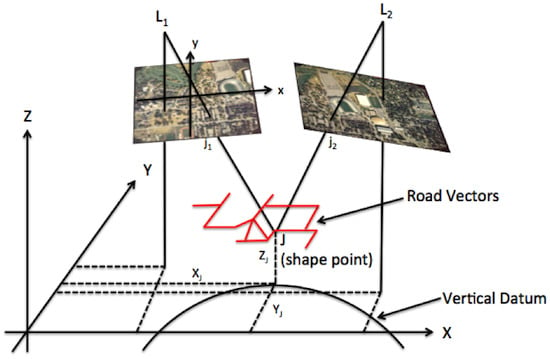
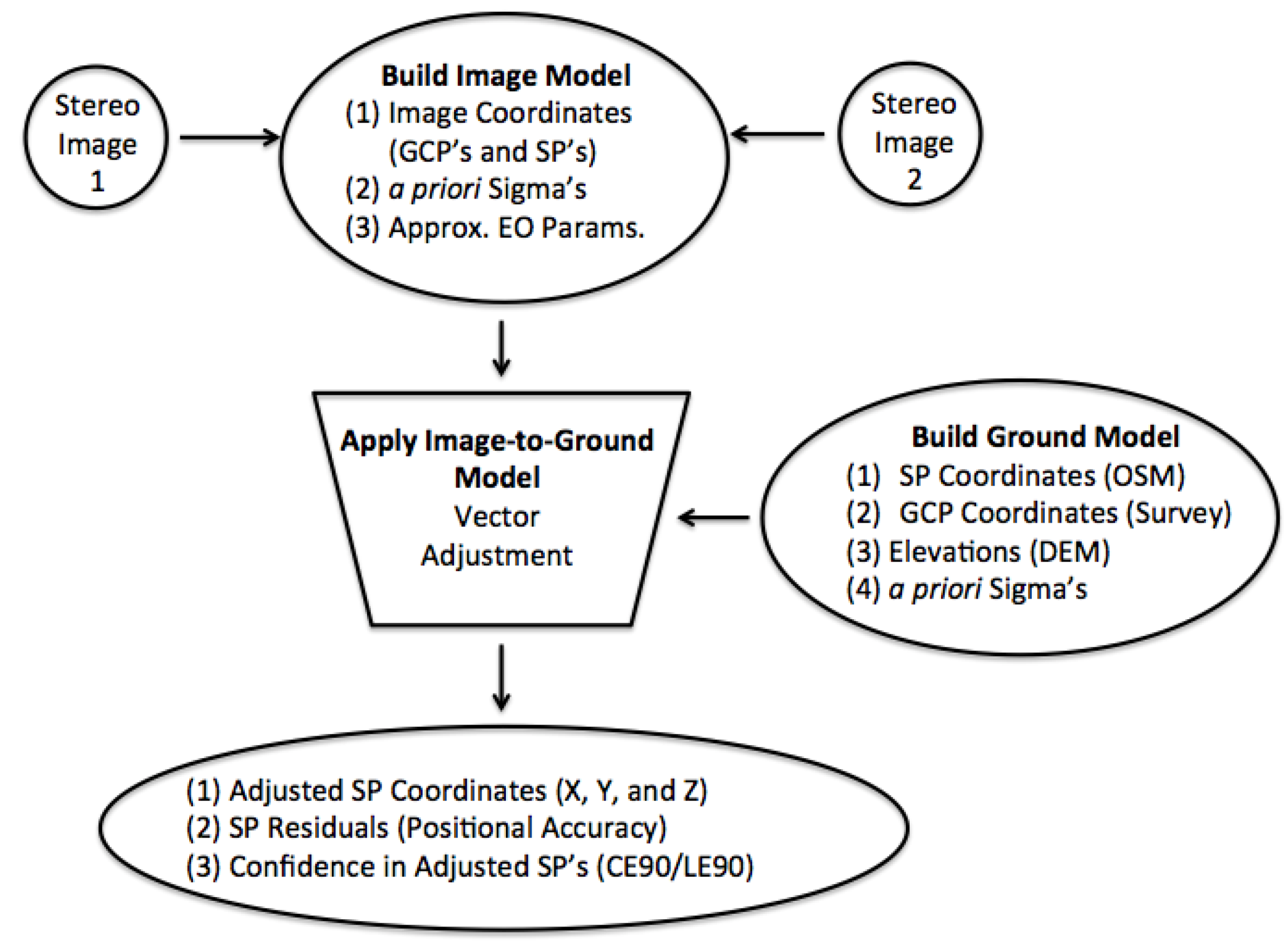
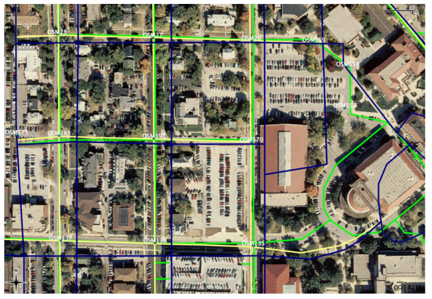
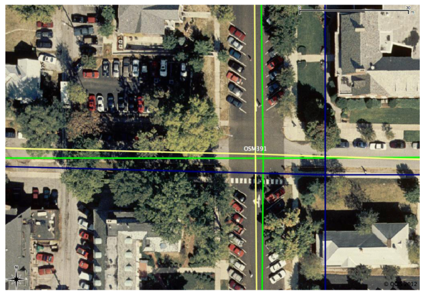
3.1. Vector Adjustment Concept
The vector adjustment model used to determine the positional accuracy of road vectors is built upon the photogrammetric bundle adjustment model and extended to include vector shape points as the object points. Since the object points are expressed in three dimensions, the elevations for the shape points are estimated using a 1/3 arc second raster Digital Elevation Model (DEM) obtained over the area of interest from the USGS National Elevation Dataset (NED) [
41]. For this research, road features from the OSM database and surveyed GCP’s were used as the object points in the adjustment to determine the positional accuracy of the vector shape points. The general idea is to use heavily weighted (well-known) GCP’s and image coordinates to establish the sensor’s exposure station and enforce the collinearity concept to solve for the true location of the OSM shape points. The adjustment residuals then describe the difference between the adjusted (“true”) location and the OSM database position. In addition, since this is a rigorous application, where the uncertainties in GCP’s, image coordinates, and object points are known, error propagation is used to compute confidence regions about the adjusted shape point locations (CE90 and LE90). The overall concept is depicted in
Figure 2.
Figure 2.
Schematic diagram of the vector adjustment concept.
Figure 2.
Schematic diagram of the vector adjustment concept.
In
Figure 2 the
SP represents the OSM shape points from the geographical database that make up a particular road vector being tested. Image coordinates of the OSM shape points are measured on each stereo image and used as input to the adjustment model. The image coordinates are considered to be well known (heavily weighted) and will ultimately control the adjusted shape point location in ground space. The assumption here is that the imagery is considered to be “truth”, either more updated or of higher importance than the OSM database location. In addition, initial approximations for the exterior orientation (EO) parameters are provided to facilitate the adjustment process, note the EO parameters are solved for in the adjustment so an initial estimate is all that is needed.
Well-known (heavily weighted) GCP’s are considered the absolute control for the adjustment. GCP’s are measured in the imagery and used with their ground space coordinates in the adjustment. Since the GCP’s are used to formulate the analytical stereo model and to create the image-to-ground relationship, it is important that they be known to a high degree of accuracy. Furthermore, it is essential for the GCP’s and OSM shape points to be referenced to the same horizontal/vertical datum and map projection to minimize any misalignment that could otherwise be removed.
The outputs from the vector adjustment are: (1) adjusted OSM shape point locations, (2) shape point adjustment residuals (which describe the positional accuracy), and (3) confidence regions about the adjusted shape point locations (CE90/LE90).
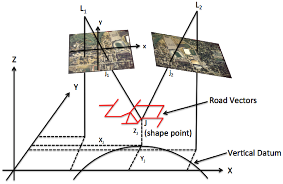
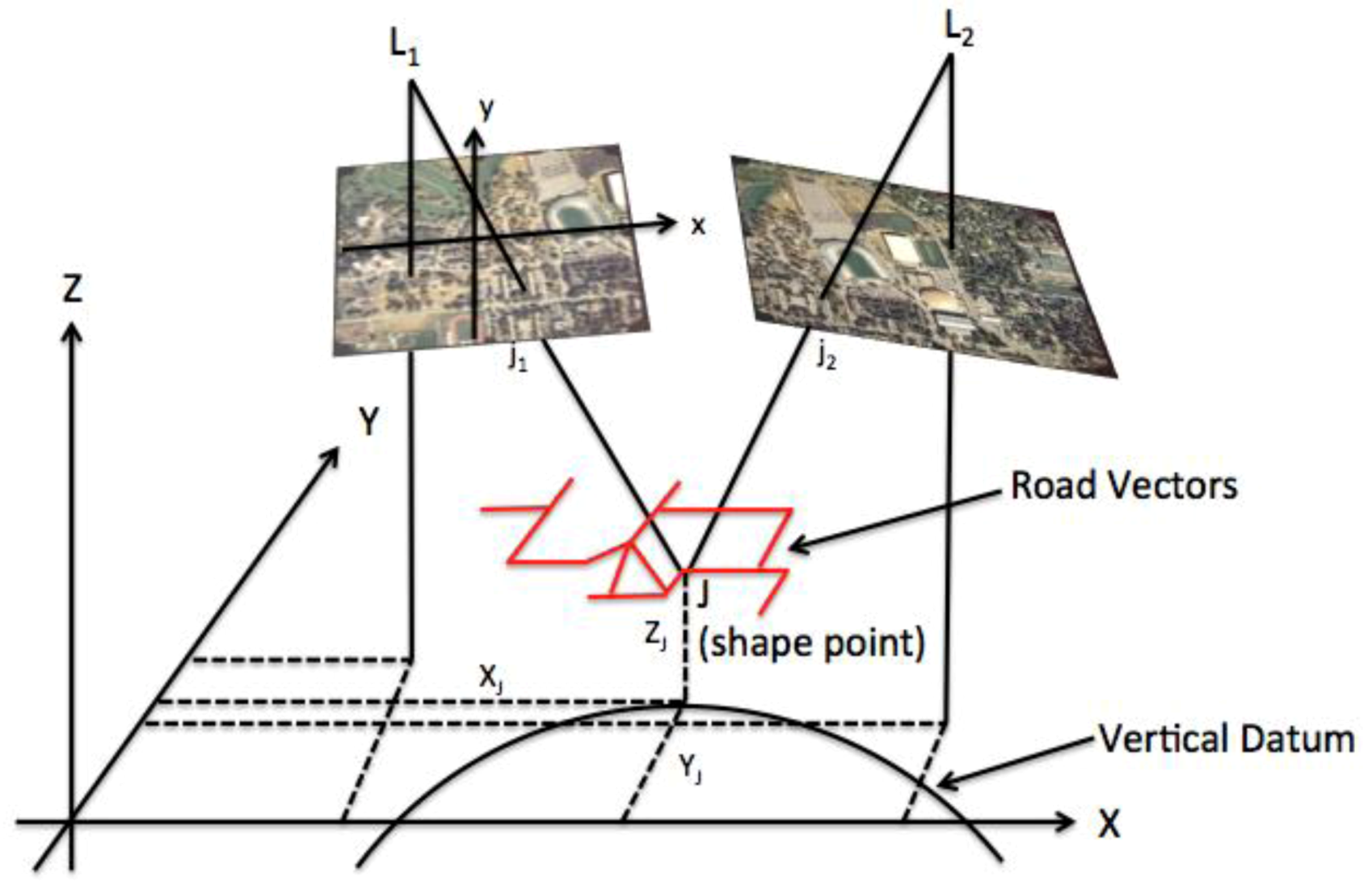
The relationship between the stereo images and an OSM shape point is an extension to the space resection problem [
42,
43]; the geometric model can be visualized in
Figure 3.
Figure 3.
Geometric diagram of the vector adjustment concept.
Figure 3.
Geometric diagram of the vector adjustment concept.
where,
L1 and
L2 are the exposure station coordinates for stereo image one and two and
j1 and
j2 are measured image coordinates of the OSM shape point,
J, on images one and two. For this work, the measuring of image coordinates was done manually,
i.e., a user measures each shape point in the stereo imagery. However, it is anticipated that this process could be automated by incorporating an image-to-vector registration process. Once the image and object space coordinates are estimated they can be used as initial approximation in the bundle adjustment model. The collinearity condition, which states that the exposure station (
![Ijgi 02 00276 i001]()
,
![Ijgi 02 00276 i002]()
,
![Ijgi 02 00276 i003]()
), an object points image derived location (
xj, yj), and the object point in ground space (
XJ,
YJ,
ZJ) all lie on a single line is used to form the observation equations in the bundle adjustment.
3.2. Photogrammetric Bundle Adjustment
The basic geometric unit in photogrammetry is the image ray, an image can be thought of as a bundle of rays converging at the perspective center with an unknown position and orientation in space [
42]. The bundles from all photos are adjusted simultaneously so that corresponding light rays from the measured image coordinates intersect at positions of the object points on the ground. The unknown quantities to be obtained from the bundle adjustment consist of the adjusted object coordinates of the vector shape points and GCP’s (
XJ,
YJ,
ZJ) and the EO parameters (
ω,
ϕ,
κ,
![Ijgi 02 00276 i001]()
,
![Ijgi 02 00276 i002]()
,
![Ijgi 02 00276 i003]()
) of all the images. The EO parameters describe the exposure station coordinates (
![Ijgi 02 00276 i001]()
,
![Ijgi 02 00276 i002]()
,
![Ijgi 02 00276 i003]()
) and the image orientation parameters (
ω,
ϕ,
κ) that are used in the collinearity equations to formulate the image-to-ground relationship.
According to Wolf and Dewitt [
43] the bundle block adjustment can be formulated using the collinearity equations, which are the foundation of the observation equations and used to form the mathematical model. The collinearity equations are documented in Equations (1) and (2) as:
where,
xj and
yj are the measured image coordinates of
J;
XJ,
YJ and
ZJ are the coordinates of object point
J,
![Ijgi 02 00276 i001]()
,
![Ijgi 02 00276 i002]()
and
![Ijgi 02 00276 i003]()
are coordinates of the image exposure station;
xo and
yo are the coordinates of the principle point known from the camera calibration report;
f is the focal length of the camera (also known from the camera calibration report); and
![Ijgi 02 00276 i004]()
,
![Ijgi 02 00276 i005]()
,…,
![Ijgi 02 00276 i006]()
are the rotation matrix terms formulated in Equation (4).
The rotation matrix terms are a result of individual rotations of
ω,
ϕ, and
κ being applied to rotations about the
x,
y, and
z-axes, respectively. The individual rotation matrices are structured as follows:
With the total rotation matrix is a result of combining the individual rotations as follows:
Since the collinearity equations are nonlinear, they are linearized by applying the first-order terms of the Taylor’s series at a set of initial approximations, a detailed derivation is provided in [
43].
The equations used to setup and solve the bundle adjustment have been well documented in several textbooks [
42,
43]. However, it is worth reviewing the basic mathematical model and matrices used to solve the system of linear equations. The general form is based on the unified least squares model and expressed as:
where,
![Ijgi 02 00276 i007]()
is a matrix of partial derivatives of the observation equations with respect to the exterior image orientation parameters (
ω,
ϕ,
κ,
![Ijgi 02 00276 i001]()
,
![Ijgi 02 00276 i002]()
,
![Ijgi 02 00276 i003]()
);
![Ijgi 02 00276 i008]()
is a vector of corrections to the exterior orientation parameters;
![Ijgi 02 00276 i009]()
is a matrix of partial derivatives of the observation equations with respect to the object point coordinates (
XJ,
YJ,
ZJ);
![Ijgi 02 00276 i010]()
is a vector of corrections to the object point coordinates (OSM shape points and GCP’s); ε
ij is the misclosure vector which is used to minimize the sum of the squared residuals; V
ij is the vector of residuals for the measured image coordinates. Adjustment residuals are important because they describe the difference between the measured and the adjusted values, which is a good indicator of how much the adjustment moved the input measurements as a result of the adjustment process.
The matrices used in the least squares model are structured as follows, for simplification the matrices are shown for a single image
i and object point
j. The
![Ijgi 02 00276 i007]()
and
![Ijgi 02 00276 i009]()
matrices are made up of terms resulting from linearizing the collinearity equations in [
43].
The
![Ijgi 02 00276 i009]()
matrix as:
The
![Ijgi 02 00276 i008]()
vector as:
The
![Ijgi 02 00276 i010]()
vector as:
The
εij vector is formulated with Taylor Series expansion terms in [
43] as:
The adjusted object points are expressed as a function of the initial measurement and the adjustment residual through the following relationship:
where,
Xj,
Yj and Zj are the unknown coordinates of point
j;
![Ijgi 02 00276 i011]()
,
![Ijgi 02 00276 i012]()
and
![Ijgi 02 00276 i013]()
are the measured coordinate value for point
j; and
![Ijgi 02 00276 i014]()
,
![Ijgi 02 00276 i015]()
and
![Ijgi 02 00276 i016]()
are the coordinate residuals for point
j. To be consistent with the collinearity equations the object point observation equations will need to be evaluated at initial approximations as follows:
With
![Ijgi 02 00276 i017]()
,
![Ijgi 02 00276 i018]()
and
![Ijgi 02 00276 i019]()
being the initial approximations for the coordinates of point
j and
dXj,
dYj,
dZj being the corrections to the approximations for coordinate point
j, as solved for in the
![Ijgi 02 00276 i010]()
matrix. Since the collinearity equations are nonlinear an iterative approach is used where corrections to the parameters are solved for and applied each time through the loop until the difference in the correction is very small or essentially unchanged. This condition is referred to as convergence. Simplifying and expressing in matrix form yields:
With
![Ijgi 02 00276 i020]()
being the difference between the current approximation and the initial approximation.
And,
![Ijgi 02 00276 i021]()
being the residual for the object point
j expressed in each component.
Weights for the object point coordinates are also used in the adjustment and based on the accuracy of the GCP’s and vector shape points. The weights for
Xj,
Yj, and
Zj object point j are expressed in matrix form as
where
![Ijgi 02 00276 i022]()
is the
a priori reference variance;
![Ijgi 02 00276 i023]()
,
![Ijgi 02 00276 i024]()
, and
![Ijgi 02 00276 i025]()
are the variances in
![Ijgi 02 00276 i011]()
,
![Ijgi 02 00276 i012]()
, and
![Ijgi 02 00276 i013]()
, respectively; and the off diagonal terms are correlation coefficients. The final types of observations used in the bundle adjustment are the EO parameters. Their observation equations take on a form similar to the object points and are given as:
And the weight matrix for the EO parameters for a single image
i is structured as:
The weights for the
x and
y image coordinates are expressed in the matrix form for an object point
j on photo
i as:
where,
![Ijgi 02 00276 i022]()
is the
a priori reference variance;
![Ijgi 02 00276 i026]()
and
![Ijgi 02 00276 i027]()
are the variances in,
xij and
yij, respectively; and the covariance
![Ijgi 02 00276 i028]()
=
![Ijgi 02 00276 i029]()
are assumed to be uncorrelated. After the individual matrices for the observation equations are formed the full set of normal equations can be structured in matrix form as:
where the matrices are formatted as:
And the Δ matrix being a combination of the corrections to the exterior orientation parameters and the corrections to the object point coordinates, with the size being determined by how many images and object points are in the adjustment.
Similarly, the
K matrix is structured as:
The submatrices used above are defined as:
With
m being the number of images,
n is the number of object points,
i is the image subscript, and
j is the object point subscript. If a point
j does not appear on image
i than a zero submatrix is used. When the normal equations are being formed it is recommended to compute the
a posteriori reference variance, which is a unit less scalar quantity that describes the uncertainty found in the observations post adjustment. It is a function of the various weight matrices (image coordinate accuracies, EO parameter accuracies, and the object point accuracies) propagated into the misclosure of the collinearity and object point observation equations. The
a posteriori standard error of unit weight can be computed as:
where
n.o. is the total number of observations and
n.u. is the total number of unknowns in the adjustment model. Once the solution converges the normal equations are then scaled by the
a posteriori reference variance to compute the final variance co-variance matrix for the adjustable parameters as:
where the resulting matrix is block diagonal with variances of the exterior orientation parameters and the object point coordinates consistent with how the
N matrix was formed. The standard deviations of the adjustment parameters are the computed by taking the square root of the diagonal variances.
3.3. Adjustment Weighting
The concept of weighting in the vector adjustment is very important and directly impacts the adjusted values, as well as the estimated uncertainty of the adjusted points. Adjustment weighting consists of assigning a numerical value to the adjustment observations and parameters based on how well the specific quantity is known. Weights are determined for both: (1) the image points, based on an a priori estimate of how well the points can be mensurated in the image, and (2) the object point coordinates, which consist of the GCP’s and vector shape point accuracies.
The general idea is the higher confidence a user has in a measurement the smaller the standard deviation will be assigned to that measurement. For example, the GCP’s used in this study were established by GPS survey, therefore the accuracies assigned to these coordinates are very small, on the order of 10-cm, or less three dimensionally. One can reason that a small standard deviation corresponds to a high user confidence in the numerical value of the measurement. On the other hand, the vector shape point coordinates were determined with less stringent methods; such as measuring a single satellite image or with a hand held GPS receiver. In this case the coordinates are much less well known, i.e., a user has less confidence in the accuracy of the point, so a standard deviation on the order of a few meters or more could be realistic.
In most cases the accuracy of the OSM shape points will not be known a priori, therefore the following approach can be implemented to estimate them. First, assign an arbitrary large standard deviation to the OSM shape points. Second, run an adjustment to determine the shape point residuals and compute the RMSE of the shape point residuals to estimate the positional displacement. Thirdly, use the RMSE value and residuals to estimate a priori standard deviations for the OSM shape points. Lastly, rerun the adjustment to compute accurate adjusted information.


 ,
,  ,
,  ), an object points image derived location (xj, yj), and the object point in ground space (XJ, YJ, ZJ) all lie on a single line is used to form the observation equations in the bundle adjustment.

 ,
,  ,…,
,…,  are the rotation matrix terms formulated in Equation (4).


 is a matrix of partial derivatives of the observation equations with respect to the exterior image orientation parameters (ω, ϕ, κ,
  is a vector of corrections to the exterior orientation parameters;
  is a matrix of partial derivatives of the observation equations with respect to the object point coordinates (XJ, YJ, ZJ);
  is a vector of corrections to the object point coordinates (OSM shape points and GCP’s); εij is the misclosure vector which is used to minimize the sum of the squared residuals; Vij is the vector of residuals for the measured image coordinates. Adjustment residuals are important because they describe the difference between the measured and the adjusted values, which is a good indicator of how much the adjustment moved the input measurements as a result of the adjustment process.


 ,
,  and
and  are the measured coordinate value for point j; and
  ,
,  and
and  are the coordinate residuals for point j. To be consistent with the collinearity equations the object point observation equations will need to be evaluated at initial approximations as follows:

 ,
,  and
and  being the initial approximations for the coordinates of point j and dXj, dYj, dZj being the corrections to the approximations for coordinate point j, as solved for in the
 being the difference between the current approximation and the initial approximation.
 being the residual for the object point j expressed in each component.

 is the a priori reference variance;
  ,
,  , and
, and  are the variances in


 and
and  are the variances in, xij and yij, respectively; and the covariance
  =
=  are assumed to be uncorrelated. After the individual matrices for the observation equations are formed the full set of normal equations can be structured in matrix form as:


