1. Introduction and Motivation
This paper identifies a specific and practical subclass of homogeneous Gaussian two-dimensional (2D) random fields and presents a simple, fast, sequential method to generate discrete realizations over a pxq (horizontal) grid for the purpose of Monte Carlo simulation-based analyses. Let us term this method Fast Sequential Simulation (FSS) for brevity of further description. FSS can be considered an extension of the sequential generation of a first order Gauss-Markov process from a 1D function of time to a 2D function of horizontal space. Although FSS was derived independently, it is also demonstrated a special case of Sequential Gaussian Simulation which is commonly used in the Geostatistics community. In particular, FSS is an unconditional simulation with simplicity and speed due to both exponential correlation in the spatial directions and an ordered generation over an evenly spaced grid of horizontal locations. Although other applications of Sequential Gaussian Simulation are more general (conditional or unconditional, irregularly spaced points, random generation paths, arbitrary valid correlation functions, etc.), many applications do not require these generalities but do require speed, preferably with a simple and direct implementation.
The paper first addresses scalar random fields, i.e., z(k, l) where z typically represents a scalar error or perturbation at grid location (k, l). The desired variance and spatial correlations for the z(k, l) are specifiable with FSS, and the multi-grid point covariance matrix derived. The paper then generalizes FSS to the generation of multivariate Gaussian two-dimensional random fields, i.e., X(k, l) , where X is a vector of arbitrary dimension n. Finally, the paper generalizes FSS results even further to non-homogeneous Gaussian two-dimensional random fields, where the variance and spatial correlations are a function of grid location (k, l). Some of the practical techniques presented for the sequential generation of both multivariate and non-homogeneous random fields are believed to be new and somewhat innovative.
Example realizations of scalar, multivariate, homogenous, and non-homogenous random fields are presented throughout the paper, as well as various theoretical properties, insights, and proofs, the latter contained in appendices. FSS is also compared to equivalent methods based on (1) Cholesky decomposition of a pre-computed a priori covariance matrix; and (2) Sequential Gaussian Simulation as implemented in various statistical packages. FSS is demonstrated to be many orders of magnitude faster than all of these other generation methods, as well as being a simpler implementation.
The ability to simulate errors across a horizontal grid with specifiable expected magnitudes (variance) and interrelationships (correlations) is an important capability in support of the Geospatial Sciences and supported by the FSS method presented in this paper. For example, the errors can represent elevation errors across a Digital Elevation database, horizontal errors in the location of vertices across a GIS database, horizontal and vertical errors in the locations of control points across a control point database, etc. All of these errors are essentially a function of horizontal location, i.e., representable as a two-dimensional random field.
These simulated errors can be used to modify corresponding “truth” data in a simulation environment. Subsequent performance of various down-stream applications can then be meaningfully assessed, including modification (tuning) of their algorithms for optimal and reliable performance. Alternatively, in an operational environment, the applications themselves can have an embedded simulation capability in order to represent the effects of errors in their input data of known (specifiable) a priori characteristics. The effect is relative to the application’s output product and usually represented graphically. The simulation of tens of millions of errors within a few seconds and hundreds of millions within 30 s on a laptop computer is desired.
Previously, relevant errors have sometimes been simulated as homogeneous errors solely as an assumption for reduced complexity and/or increased speed. However, many realistic applications correspond to data with non-homogeneous error characteristics; for example, data sets previously fused from other data sets with differing error (accuracy) characteristics. This paper addresses both types of errors. The non-homogeneous techniques presented in this paper essentially preserve the speed associated with the technique presented for the homogeneous case, typically reducing the speed by only a factor of two or three. The corresponding non-homogeneous characteristics are not totally general, but still adequate for many applications.
Finally, a common theme throughout this paper is the practical computation and need for a multi-grid point covariance matrix corresponding to z(k, l) or X(k, l) at multiple grid point locations. It is used by various applications to predict the accuracy of their input data and properly weight it within their various algorithms.
The authors of [
1,
2,
3,
4,
5] discuss random fields in general, including their generation or simulation. Generation techniques include those based on Cholesky decomposition and Sequential Gaussian Simulation. In addition, these references discuss interpolation of a random field’s realization based on Kriging. These references are relatively standard in the geostatistics community. They, along with other references from this community, are referenced per specific topic throughout the remainder of this paper, including appendices.
As detailed later, FSS was derived independently of Gaussian Sequential Simulation but is equivalent in specified circumstances. FSS is also directly related to both generalized multi-grid point covariance matrices [
6] and strictly positive definite correlation functions [
7] that have applications in the Geospatial community. Recent applications of FSS include evaluating conflation methods [
8] and various geospatial algorithms [
9].
Roadmap
Section 1,
Section 2,
Section 3 and
Section 4 of this paper define the scalar homogeneous Gaussian 2D random field, the fast sequential generation algorithm FSS, and related practical aspects.
Section 5 compares FSS to more typical generation methods such as those based on Cholesky decomposition or Sequential Gaussian Simulation, particularly with respect to timing or throughput.
Section 6 then extends the FSS technique to a multivariate homogeneous Gaussian 2D random field, and
Section 7 to a non-homogeneous Gaussian 2D random field.
2. A Scalar Gaussian 2D Random Field and Its Sequential Generation
In this section of the paper, we define a scalar, homogeneous, Gaussian two-dimensional (2D) random field, typically corresponding to perturbations or errors. We also present FSS, the algorithm for the fast and sequential generation of a discrete and specific realization of this random field that can be used for various Monte Carlo simulation-based analyses.
We assume that the random field corresponds to z-error for specificity. Indices k and l correspond to a two-dimensional grid in the y-x horizontal plane: k is in the “y” direction and is the first grid index, l is in the “x” direction and is the second grid index. Specifically, z(k, l) corresponds to z-error in meters at grid point (k, l).
2.1. Statistical Characteristics
z(
k, l) is normally (Gaussian) distributed, and has a mean value of zero and a specifiable one-sigma
σz,
i.e., is normally distributed
N(0,
σz) for all grid locations (
k, l). Its spatial correlation across the grid is separable,
i.e., has the (normalized) correlation function
ρ(
∆k, ∆l), where
∆k and
∆l are the absolute values of the component-wise differences in the (
k, l) location of two arbitrary grid points. This function is represented as:
where
Ty and
Tx are specifiable spatial correlation distance constants (meters) and
δy and
δx specifiable grid spacing (meters) in the
y and the
x directions in the horizontal plane, respectively. Note that
∆y = ∆kδy and
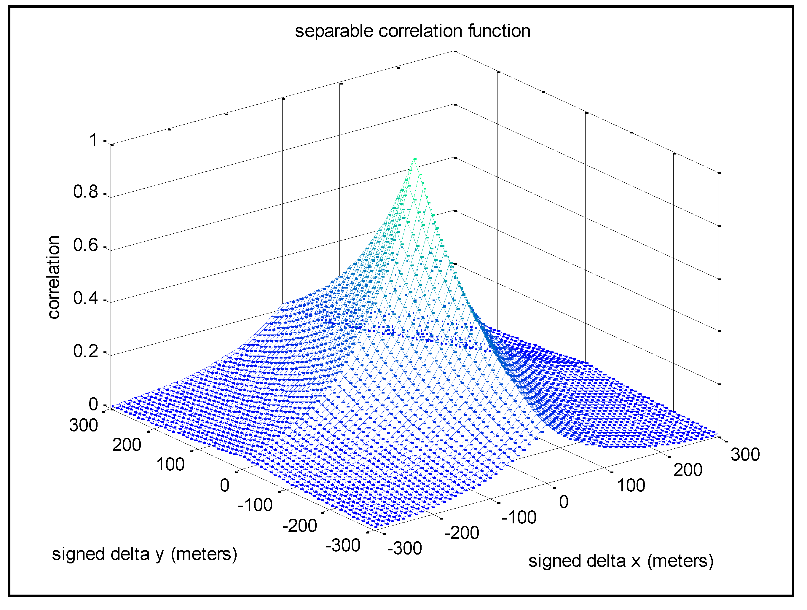
∆x = ∆lδx Figure 1 presents an example of
ρ(
∆y, ∆x), with
Ty = 200 m,
Tx = 100 m, and
δy =
δx = 10 m. The spatial correlation
ρ(
∆y, ∆x) is applicable to any pair of grid points within the entire grid that are separated by
∆y meters in the
y-direction and
∆x meters in the
x-direction. The use of two different spatial correlation distance constants allows for specification of different correlation characteristics in each of the horizontal directions.
Figure 1.
An example of the separable spatial correlation function; in the plot of ρ(∆y, ∆x), ∆y and ∆x have signed values.
Figure 1.
An example of the separable spatial correlation function; in the plot of ρ(∆y, ∆x), ∆y and ∆x have signed values.
Regarding the
a priori statistics of
z(
k, l) in a more formal manner:
at an arbitrary location (
k, l) within the grid.
Note that
E{} is the expectation operator, and
∆k ≥ 0,
∆l ≥ 0,
Ty > 0,
Tx > 0,
δy > 0,
δx > 0, |
ρ(
∆k, ∆l)| ˂ 1 if
∆k ≠ 0 or
∆l ≠ 0, and
ρ(
∆k, ∆l) = 1 when
∆k =
∆l = 0.
Section 3.0 of this paper also presents the covariance matrix associated with two or more
z(
k, l), each associated with a different grid point (
k,l).
2.2. Core Grid-Generation Equation
Equation (3) is the core grid-generation equation for FSS:
The integers
k and
l correspond to points in the grid,
s =
e−δy/Ty, and
r =
e−δx/Tx.
u(k, l) is a random sample of Gaussian white noise, and is normally distributed
N(0,
σu), where
![Ijgi 03 00817 i002]()
. That is, given a desired
s,
r, and
σz, a corresponding value of
σu is computed per the above.
s is the spatial correlation of the scalar error
z between adjacent grid points in the
k (or
y) direction (0 ≤
s ≤ 1, unit-less), and
r is the spatial correlation of the scalar error between adjacent grid points in the
l (or
x) direction (0 ≤
r ≤ 1, unit-less) Therefore, we can also write the spatial correlation function
ρ(
∆k, ∆l) as a function of grid units only:
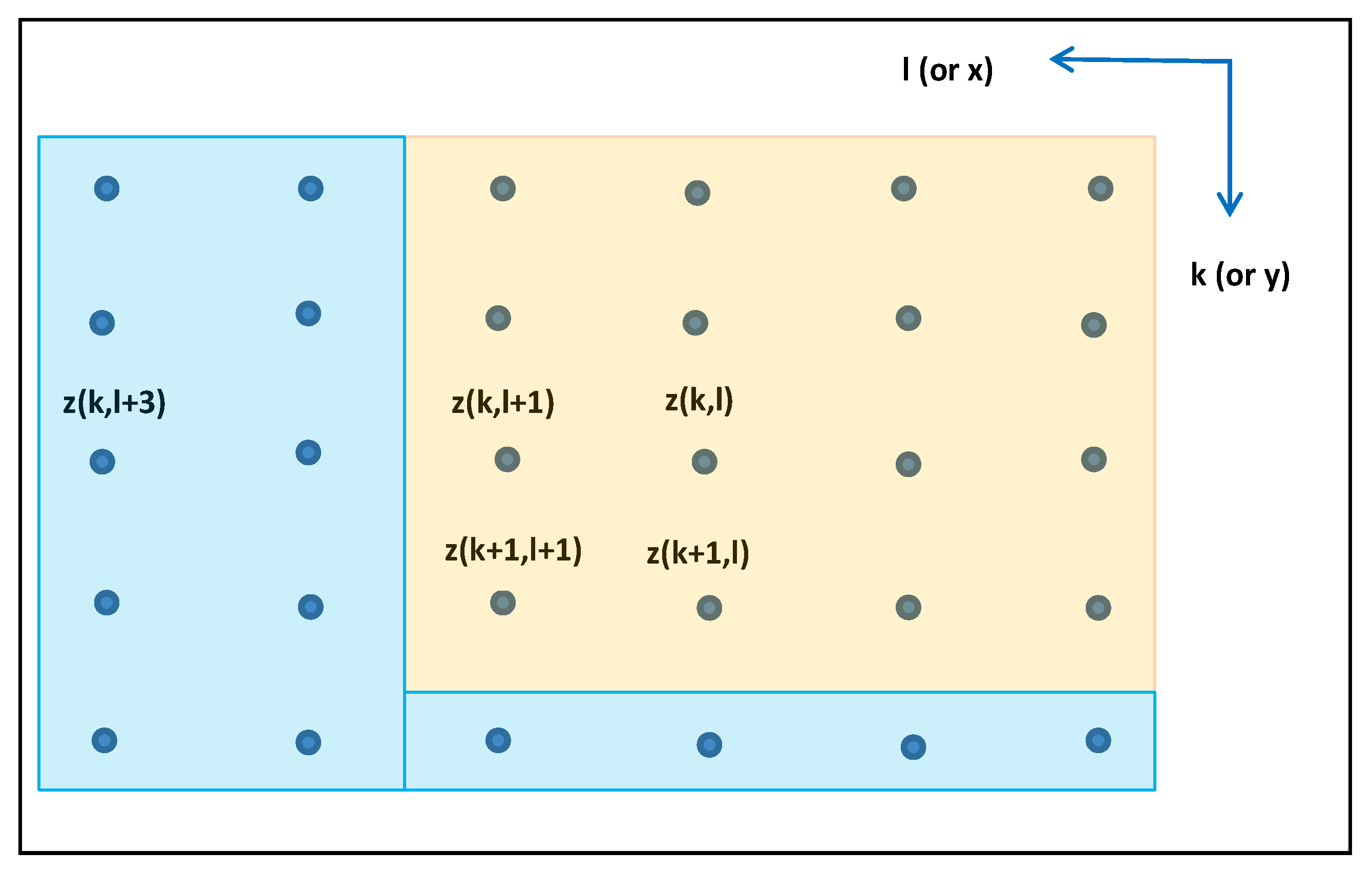
Figure 2 illustrates the grid of errors
z(
k, l) generated based on Equation (3) and corresponding to a specific realization of the scalar, homogeneous, two-dimensional random field.
Figure 2.
Horizontal grid of z errors.
Figure 2.
Horizontal grid of z errors.
All errors in the light orange area affect the error
z(
k + 1,
l + 1)and those in the light blue area do not. Also, based on the specific sequential grid generation algorithm presented in
Section 2.3, an error in the light blue area (e.g.,
z(
k,
l + 3)) may be generated prior to
z(
k + 1,
l + 1) even though it does not affect it.
2.3. Sequential Generation Algorithm for Realization over a pxq Grid
The following presents a specific FSS algorithm for a discrete realization of
z(
k, l) over a
pxq grid based on Equation (3):
z(1,1) = random_N(0, σz);
z(2,1) = sz(1,1) + random_N(0, σu);
z(1,2) = rz(1,1) + random_N(0, σu);
z(2,2) = rz(2,1) + sz(1,2) − rsz(1,1) + random_N(0, σu);
z(1,q) = rz(1,q-1) + random_N(0, σu);
z(2,q) = rz(2, q-1) + sz(1, q) − rsz(1, q-1) + random_N(0, σu);
The above completes rows 1 and 2. Generate row 3 as follows:
z(3,1) = sz(2,1) + random_N(0, σu);
z(3,2) = rz(3,1) +sz(2,2) − rsz(2,1) + random_N(0, σu);
z(3,q) = rz(3, q − 1) + sz(2, q) − rsz(2, q − 1) + random_N(0, σu);
Repeat row 3-type processing for rows 4 through p.
Note that, in general, “random_N(0, σa)” corresponds to a random number (realization) from a N(0, σu) probability distribution; for example, in matlab this is implemented as “sigma_a * randn(1,1)”.
Appendix A of this paper presents a direct proof that the above FSS algorithm generates a realization of a two-dimensional random field with the specifiable statistical properties presented in
Section 2.1.
Appendix B also demonstrates its mathematical equivalence to a corresponding Sequential Gaussian Simulation approach for completeness. The latter must specify separable exponential correlation in the spatial directions and a fixed grid with a specific ordered path across it for generation of the realization. Also, depending on how it is implemented, it may or may not take advantage of the need to use the realization at only three previously generated grid points for generation at the current grid point, as does FSS. If it did in an efficient manner using pre-computed Kriging weights and little overhead due to flexibility and complexity, its speed could approach that of FSS.
2.3.1. Grid Spacing
Equation (3) and the above algorithm should typically incorporate grid spacing δy and δx equivalent to approximately one-ninth or less their respective spatial correlation distance constant, insuring at least 0.9 correlation with an adjacent grid point, i.e., s = e−δy/Ty ≥ e−1/9 ≅ 0.9 and r = e−δx/Tx ≥ e−1/9 ≅ 0.9, or equivalently, δy ≤ Ty/9 m and δx ≤ Tx/9 m. Of course, this “rule-of-thumb” is application dependent. For example, if very high spatial correlation between adjacent grid points is of interest, spacing should be closer.
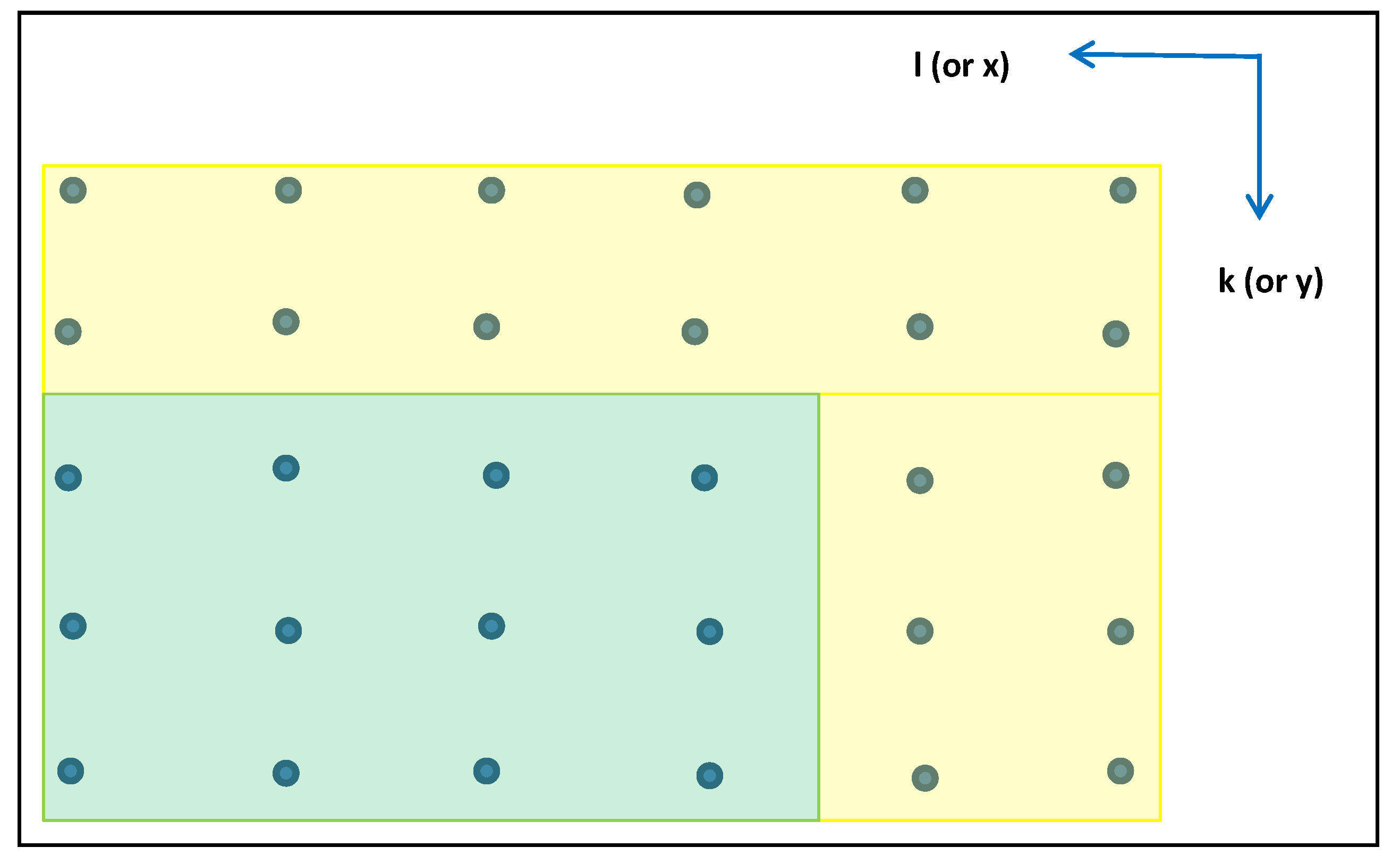
2.3.2. Grid Buffer
As shown in
Appendix A of this paper, the statistical properties of the
z(
k, l) are based on steady-state properties over an assumed infinite horizontal grid. Thus, for an actual application (realization) necessarily using a finite grid, the “final” grid should have a “buffer” on two edges of the computed grid to ensure that steady-state has essentially been reached. This is illustrated in
Figure 3, where the buffer is yellow and the final grid is green.
Figure 3.
Grid buffer (yellow), computed grid (yellow + green), final grid (green).
Figure 3.
Grid buffer (yellow), computed grid (yellow + green), final grid (green).
Placement of the buffer corresponds to the specific sequential grid generation algorithm presented earlier that starts at the top of the grid and always proceeds from right to left. The width of the top buffer should correspond to the equivalent of approximately two times the spatial correlation distance constant in the y-direction, and the width of the side buffer should correspond to the equivalent of approximately two times the spatial correlation distance constant in the x-direction.
More specifically,
width of top buffer (#
grid rows) =
![Ijgi 03 00817 i003]()
and
width of side buffer (#
grid columns) = 2
Tx/
δx. Or equivalently, if
s and
r equal the value 0.9, 19 grid rows and 19 grid columns. This will ensure generation of errors throughout the final grid with the desired statistical properties.
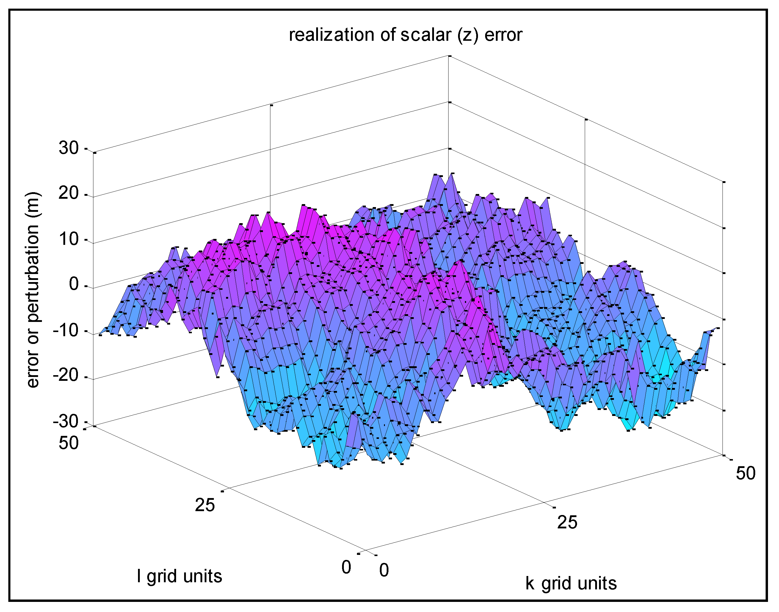
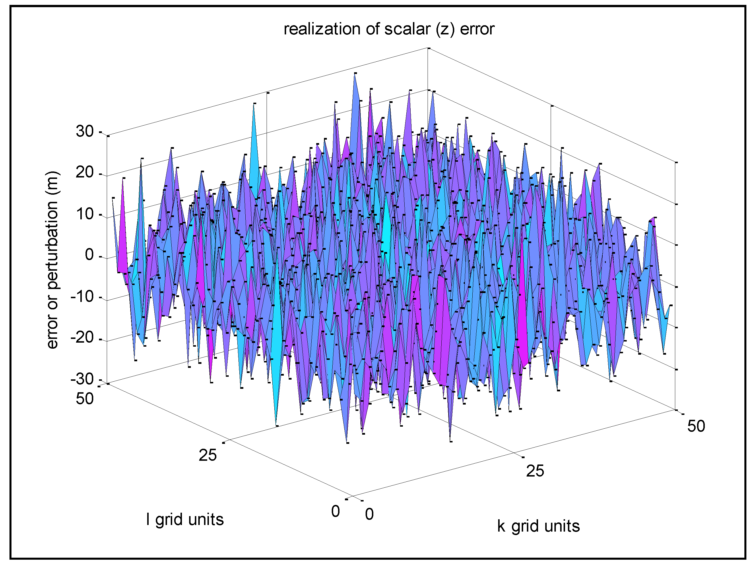
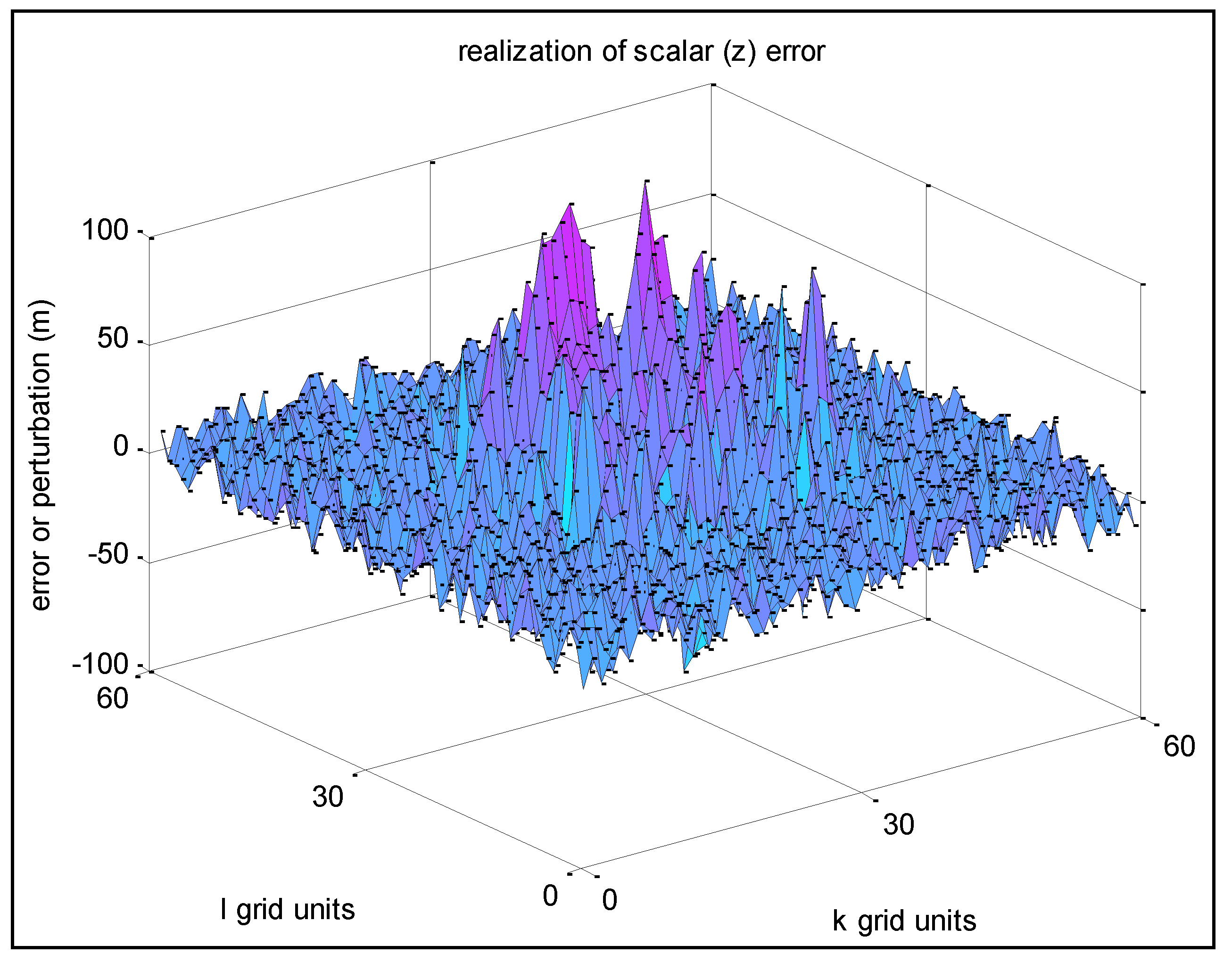
2.4. Example Realizations: Surface Plots
This section presents surface plots of the
z-error over a subset of a 2D final grid generated using the sequential algorithm of
Section 2.3. Example 1 corresponds to specified
σz = 10 m, and specified
s =
r = 0.95 (thus
σu = 0.975 m). Assuming a grid spacing in both the y and x directions of 1 m (
δy =
δx = 1), this corresponds to spatial distance constants equal to
Ty =
Tx = 19.5 m.
In this particular case, the spatial distance constants Ty and Tx were derived from the specified s and r, given assumed grid spacing δy and δx not vice versa. The spatial distance constants were computed for information only. That is, there are two basic but equivalent approaches for the specification, application, and interpretation of spatial correlation, the particular approach selected based on convenience:
Approach 1—specify spatial correlation by the values of s and r (unitless) directly, implement Equation (3), and then interpret location-dependent results in terms of grid units. Given assumed grid spacing δy and δx (meters), the spatial distance constants Ty and Tx (meters) can be derived for information purposes only.
Approach 2—specify spatial correlation by the values of Ty and Tx (meters) and grid spacing δy and δx (meters), compute s and r, implement Equation (3), and then interpret location-dependent results in terms of y-x horizontal space in meters. The approach works well when the generated random field is to correspond to the a priori statistics and spatial resolution of a specific application of interest in the Geospatial Sciences.
Figure 4 presents the realization results of Example 1 based on Approach 1. Note that the remaining realization examples in this paper use Approach 1 as well, as it is most convenient.
Figure 4.
Example 1—Realization of z-error with high spatial correlation between adjacent grid points.
Figure 4.
Example 1—Realization of z-error with high spatial correlation between adjacent grid points.
Figure 5 corresponds to Example 2, a new realization with the same
σz = 10 m, but with
s =
r = 0.1 (thus
σu = 9.9 m).
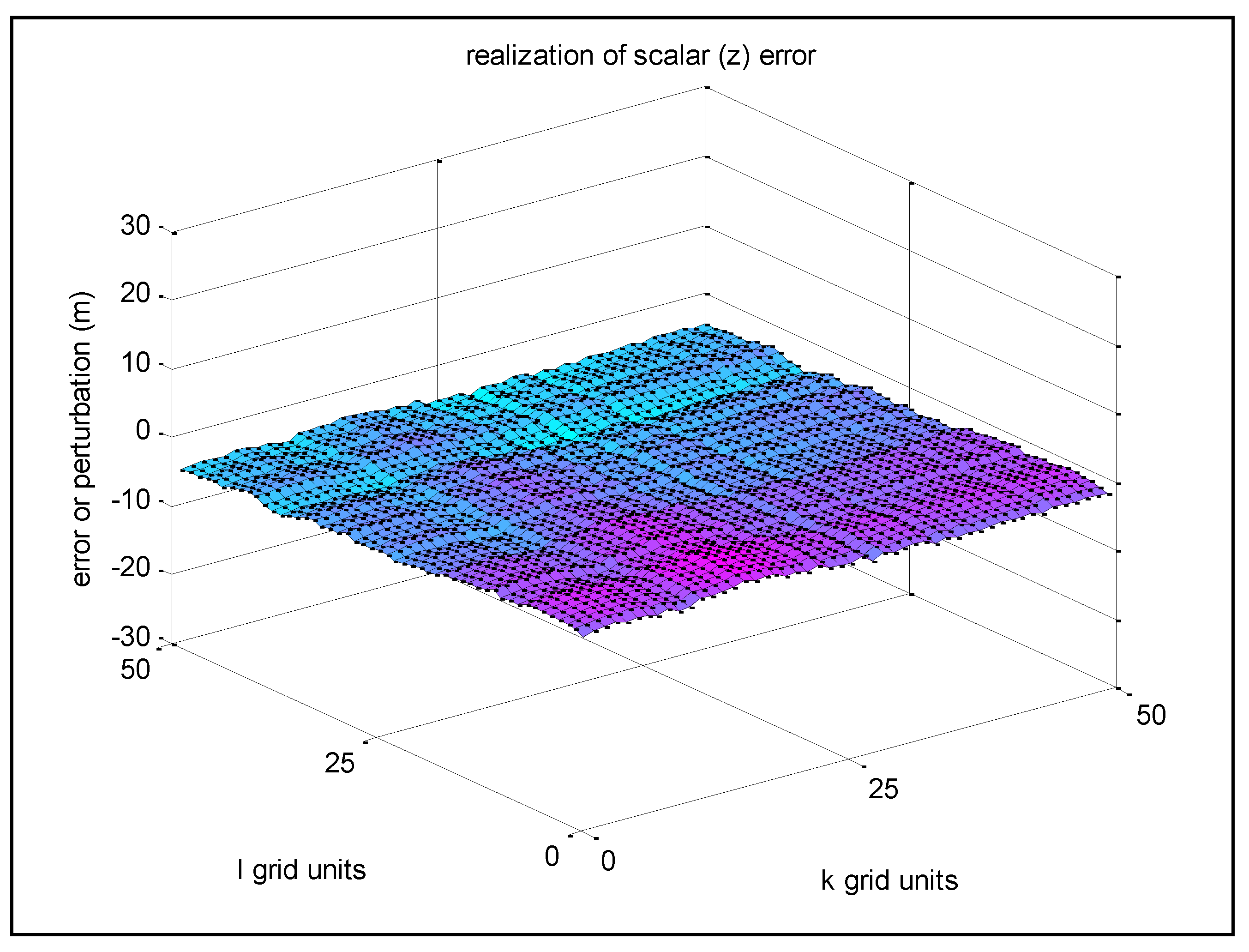
Figure 6 corresponds to Example 3, a new realization with the same
σz = 10 m, but with
s =
r = 0.999 (thus
σu = 0.02 m).
As expected, the above realizations over portions of the grid do not have a mean z-error of zero nor a standard deviation about the mean of 10 m. However, when sample statistics are computed over numerous realizations, the corresponding mean and standard deviation approach 0 m and 10 m, respectively, matching the common a priori statistics used to generate the realizations.
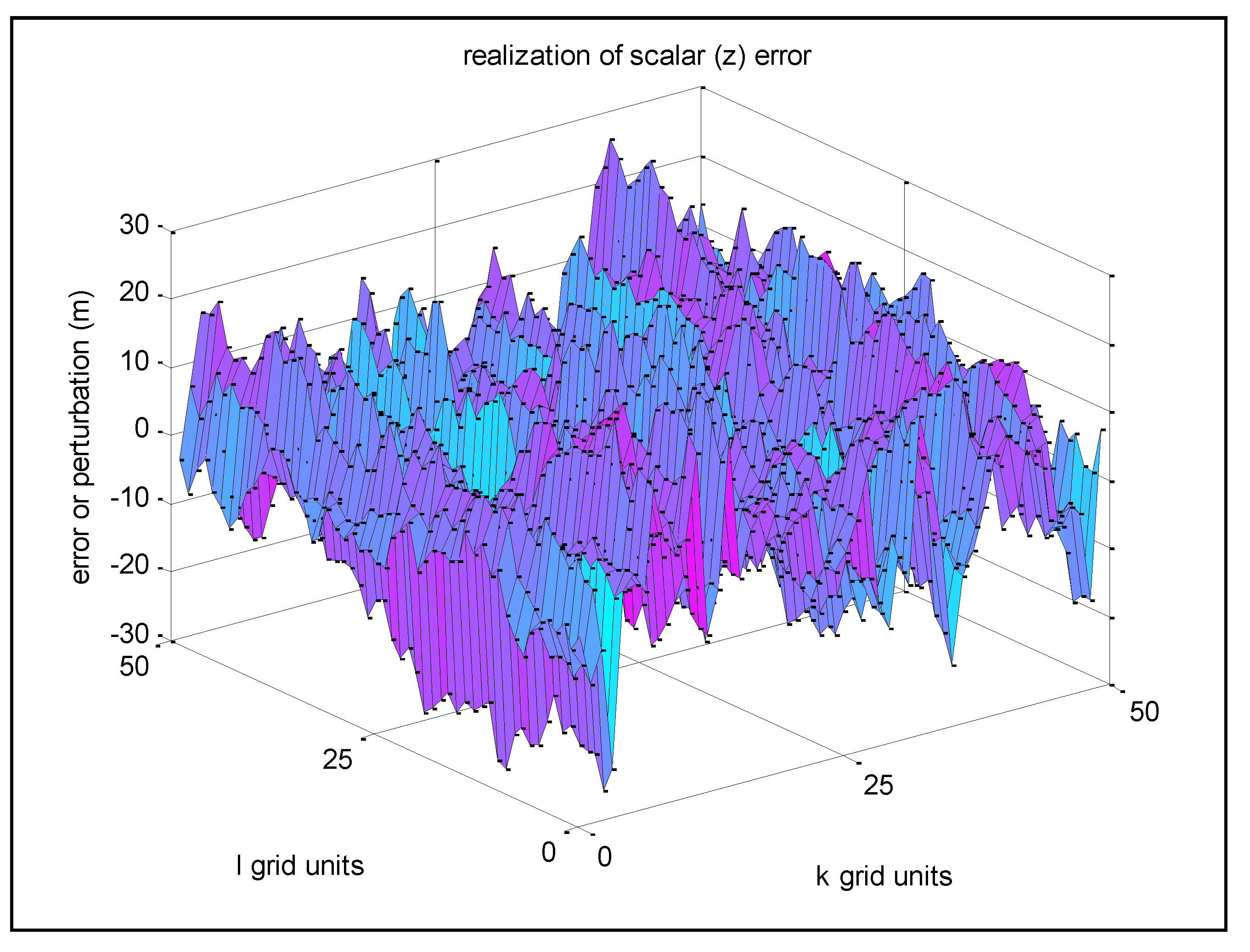
Finally,
Figure 7 below presents Example 4, a new realization with the same
σz = 10 m, but with
s = 0.1 and
r = 0.95 (thus,
σu = 3.107),
i.e., different spatial correlations in the two directions.
Figure 5.
Example 2—Realization of z-error with low spatial correlation between adjacent grid points.
Figure 5.
Example 2—Realization of z-error with low spatial correlation between adjacent grid points.
Figure 6.
Example 3—Realization of z-error with very high spatial correlation between adjacent grid points.
Figure 6.
Example 3—Realization of z-error with very high spatial correlation between adjacent grid points.
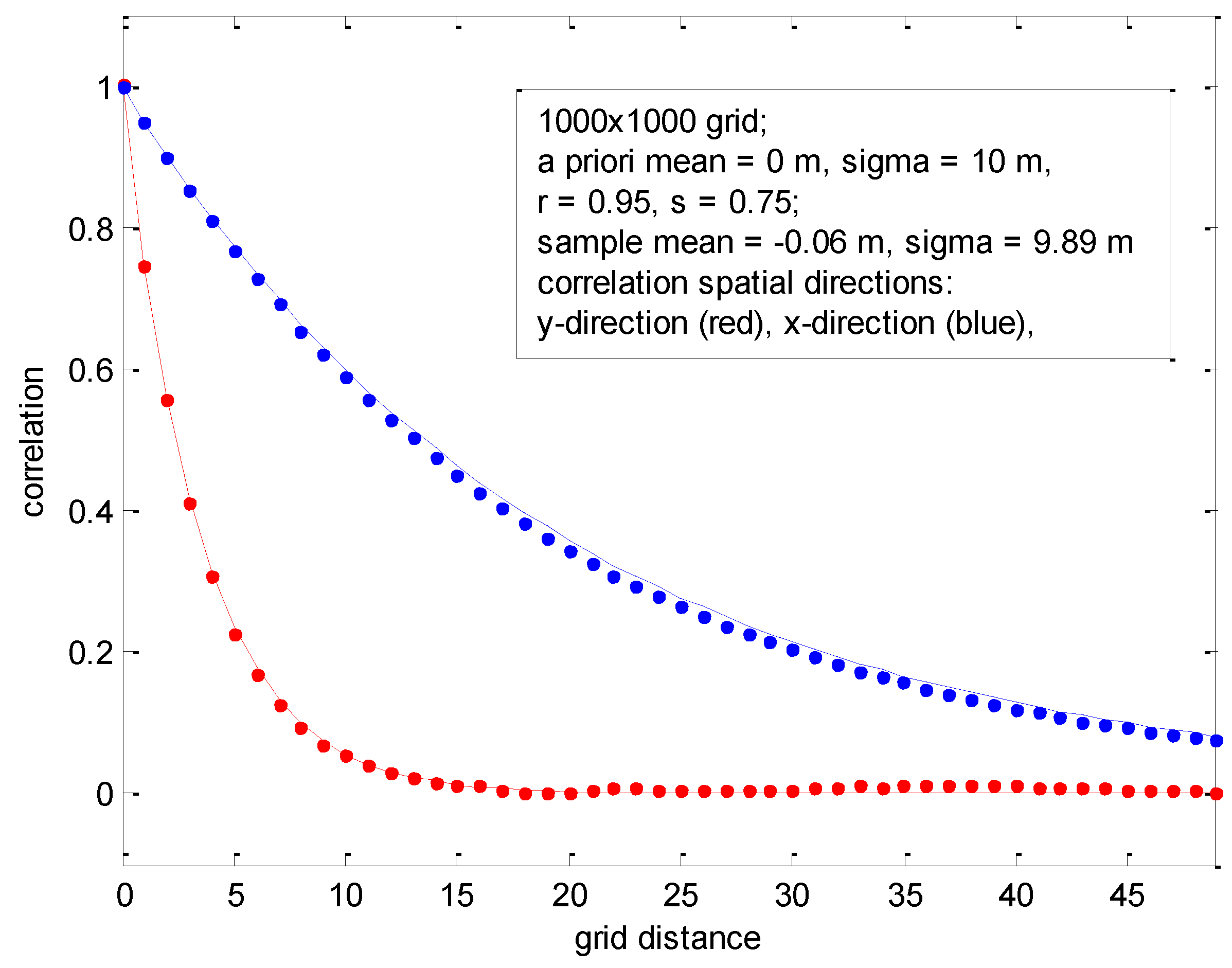
2.5. Example Realizations: Sample Statistics
Sample correlation functions or correlograms were computed for two independent realizations across a final z-grid 1000 × 1000 in size.
A priori statistics were specified with a fixed mean value of 0 and a standard deviation about the mean of
σz = 10 m. The first realization corresponded to
a priori correlations represented by
r = 0.95 and
s = 0.75, and is presented in
Figure 8. Correlation functions were plotted as a function of horizontal distance in the x-direction and horizontal distance in the y-direction, and are different as expected per the values of r and s.
Figure 7.
Example 4—Realization of z-error with different spatial correlations.
Figure 7.
Example 4—Realization of z-error with different spatial correlations.
Figure 8.
Sample statistics corresponding to 1000 × 1000 grid with different a priori correlations.
Figure 8.
Sample statistics corresponding to 1000 × 1000 grid with different a priori correlations.
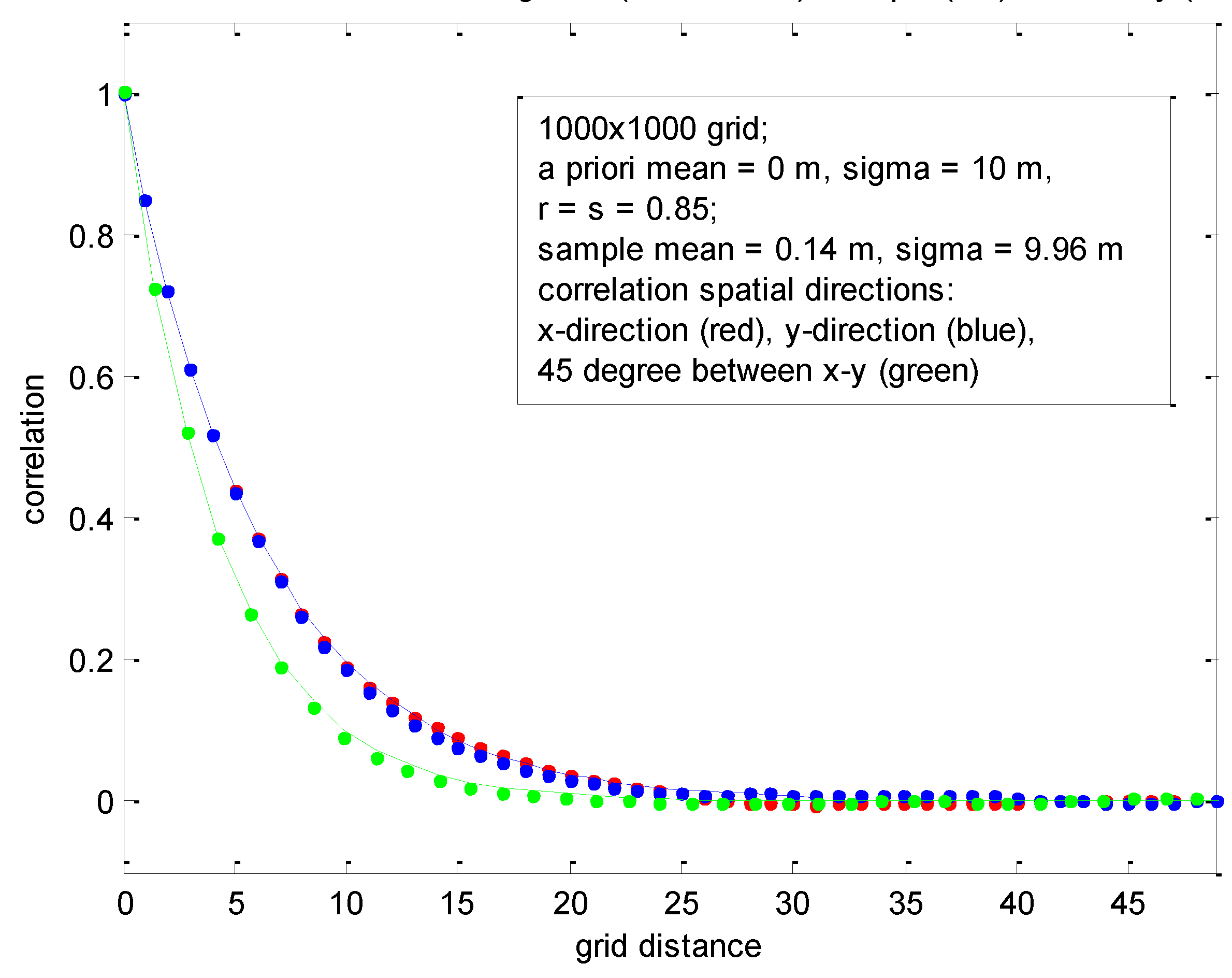
The second realization corresponded to
r =
s = 0.85, and is presented in
Figure 9. Three different horizontal directions were evaluated: x, y, and 45 degrees between. Note that results for the latter are different even though
r =
s because the FSS correlation model is not isotropic. (Note that 45 degrees yields the direction with maximum difference.) In general, both plots demonstrate nearly identical results between the true and sample correlation functions—not unexpected because FSS has virtually no approximations and because the random field is ergodic and the number of samples within a given realization large.
Figure 9.
Sample statistics corresponding to 1000 × 1000 grid with the same a priori correlations for the x and y directions, evaluated across three different directions.
Figure 9.
Sample statistics corresponding to 1000 × 1000 grid with the same a priori correlations for the x and y directions, evaluated across three different directions.
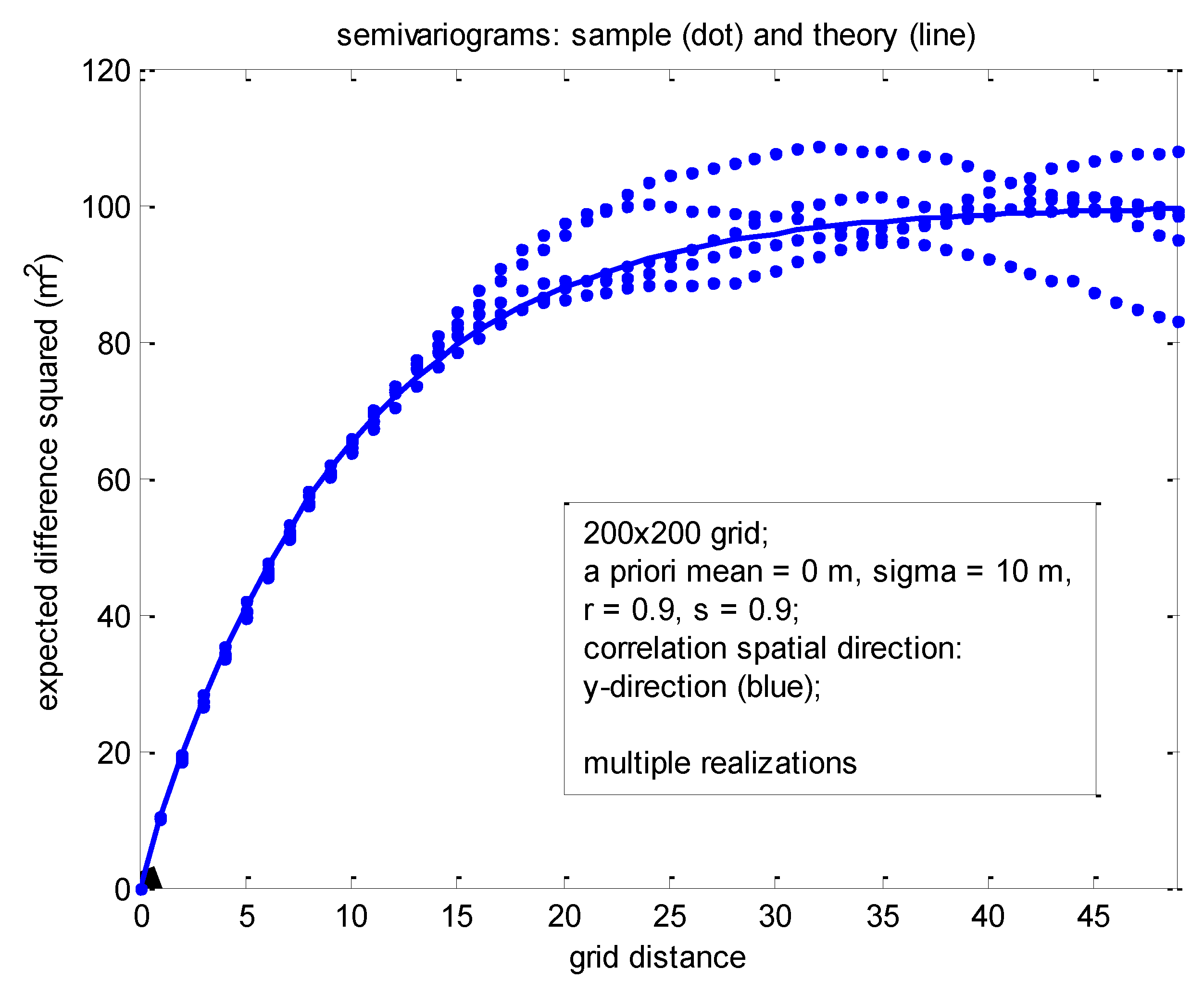
Figure 10.
Semivariograms corresponding to 200 × 200 grid with the same a priori correlations for the x and y directions, evaluated across the y-direction for five different realizations.
Figure 10.
Semivariograms corresponding to 200 × 200 grid with the same a priori correlations for the x and y directions, evaluated across the y-direction for five different realizations.
Figure 10 corresponds to a set of five independent realizations, this time over a much smaller 200 × 200 grid.
A priori statistics were identical to those corresponding to
Figure 9 except that
r =
s = 0.9. Also, the sample and theoretical statistics computed correspond to the semivariogram, typically of interest in the geostatistics community, computed in the y-direction across the horizontal grid. (See [
5] for example, definitions of the correlogram and semivariogram.) Note the reasonable variability of the sample semivariograms corresponding to each of the five realizations about the common theoretical semivariogram.
3. Multi-Grid Point Covariance Matrix
If there are
m specific scalar errors
z(
k, l) of interest associated with
m arbitrary and different grid locations (
k, l), their corresponding
m ×
n (joint) covariance matrix is symmetric and positive definite (valid) since all the grid point errors have the same variance
![Ijgi 03 00817 i004]()
and have inter-grid point correlation between pairs corresponding to a normalized strictly positive definite correlation function (spdcf)
ρ(
∆k, ∆l) =
ρ(
∆y, ∆x) =
e−∆lδy/Tye−∆kδx/Tx,
i.e., the multi-grid point covariance matrix equals:
where
Z is an
mx1 vector such that
ZT = [
z1, …,
zm] and the
zi =
z(
ki, li),
i = 1,…,
m, correspond to an ordered list of the
m grid point locations. Also,
∆yij =
∆yji and
∆xij =
∆xji are the y and x distances in meters in the horizontal plane between the ordered points
i, j ∈ {1,…,
m};
![Ijgi 03 00817 i004]()
directly multiplies each element of the
mxm matrix. (Alternatively, the spatial correlation function and distances could have been written based on grid units.)
Note that the above is an
a priori covariance matrix corresponding to the various
z(
k, l) considered as random variables, not specific realizations. See Reference [
7] regarding the properties of a spdcf such that the above
mxm P is guaranteed a valid (symmetric and positive definite) covariance matrix regardless the size of
m. In general, just because the absolute value of correlation between two arbitrary grid point locations is less than 1.0, this by itself does not ensure a valid multi-grid point covariance matrix for
m > 2.
The FSS generation of a realization of
z(
k, l) over a 2D grid as presented in
Section 2.3 did not require use of the explicit multi-grid point covariance matrix in the generation process. So, why is the calculation of this covariance matrix of interest in terms of specific applications of generated errors or perturbations? A major reason is as follows: An “analysis module” may generate the simulated grid of errors and apply a subset to “truth data” and then pass the composite data to a “down-stream” application such that its performance can be assessed in the presence of errors. Many such applications also require knowledge of the multi-grid point covariance matrix corresponding to the composite data for purposes of proper weighting of the composite data in various estimation procedures (Kalman Filter and Weighted Least Squares estimators) for the parameters (state vectors) of interest to the application [
6]. Of course, these applications can simply be passed, along with the composite data, the corresponding
![Ijgi 03 00817 i004]()
and the parameters that define
ρ (
∆k, ∆l) =
ρ(
∆y, ∆x) =
e−∆lδy/Tye−∆lδx/Tx, such that the applications can then build the appropriate multi-grid point covariance matrix themselves.
Homogeneity and Gaussian Joint Probability Density
The scalar errors
z(
k, l) generated using the FSS sequential generation technique are Gaussian distributed as they are a linear combination of the
u(
k, l), which are Gaussian distributed by definition. (The linear combination is demonstrated explicitly in
Appendix A.) Also, the corresponding grid of
z-errors corresponds to a wide-sense homogenous random field since the variance and correlation of errors are invariant of specific absolute grid location(s). In addition, since the errors are Gaussian distributed, a wide-sense homogeneous random field is equivalent to a homogeneous random field [
2].
Any finite collection of
z(
k, l) at different grid locations (
k, l) contained in the
mx1 vector
Z has a corresponding Gaussian joint probability density function defined as follows:
where
P is the multi-grid point covariance matrix, and
det is the matrix determinant. Thus, probabilities can be assigned in a straightforward manner to any absolute or relative confidence interval of interest.
Finally, it is worth noting that all of the multi-grid point covariance matrices computed per this paper are valid, regardless the specific underlying probability distribution of errors. This is true for both the scalar error of
Section 1,
Section 2,
Section 3 ,
Section 4 and
Section 5, multivariate errors of
Section 6, and non-homogenous errors of
Section 7. This is discussed in References [
6,
7], which also allow for the use of any valid family of spdcf. In addition, the authors of [
6] discuss the importance of such covariance matrices, other generation methods for such covariance matrices, and how to generate corresponding probability error ellipsoids. Note that in Reference [
6], these covariance matrices are more generally termed “multi-state vector error covariance matrices”.
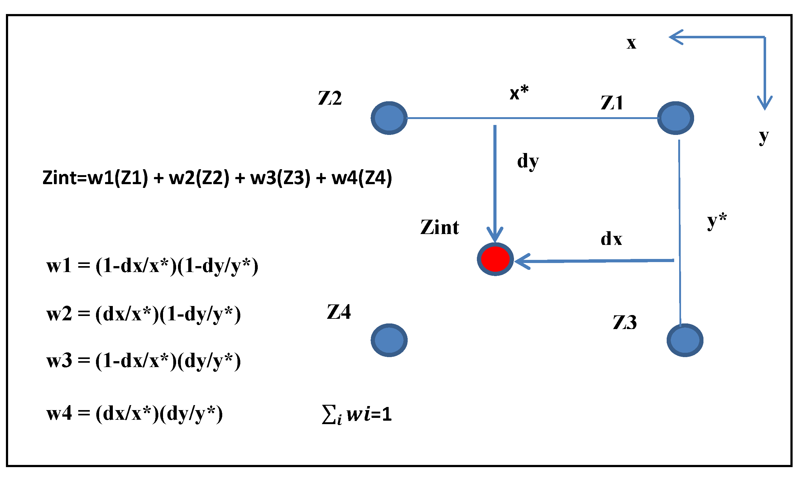
4. Interpolation into the Grid
The FSS technique as described in
Section 1 and
Section 2 of this paper generates a realization of a random field at grid point locations only. This is perfectly adequate for many applications since the grid can be very large and dense. However, if scalar errors are desired between grid point locations, interpolation of the
z(
k, l) at the four enclosing grid point locations may be performed. Also, the multi-grid point covariance (Equation (5)) can be easily modified for a corresponding set of interpolated points. Simply modify the distances between grid points to corresponding distance between the locations of the interpolated points. These distances may be represented in either non-integer units of grid spacing or corresponding
y and
x distances in meters in the horizontal plane.
5. Comparison to Alternate Generation Methods
This paper presents FSS, a fast and efficient sequential method for the generation of a 2D grid of errors or perturbations. There is also an implied, associated multi-grid point covariance matrix (e.g., Equation (5)), but this covariance matrix is not needed in the generation process. On the other hand, the spatial correlation of errors with this generation method is limited to a specific spdcf family of spatial correlation functions, i.e., ρ (∆k, ∆l) = ρ(∆y, ∆x) = e−∆kδy/Tye−∆lδx/Tx. (Albeit, reasonably general in that the distance constants Ty and Tx are specifiable).
There are two other general approaches to the generation (simulation) over a 2D grid: (1) matrix square roots; and (2) Sequential Gaussian Simulation. The latter is sequential and, as mentioned previously, more general than FSS. The former is also more general, but not sequential. They are described in more detail in the next subsection.
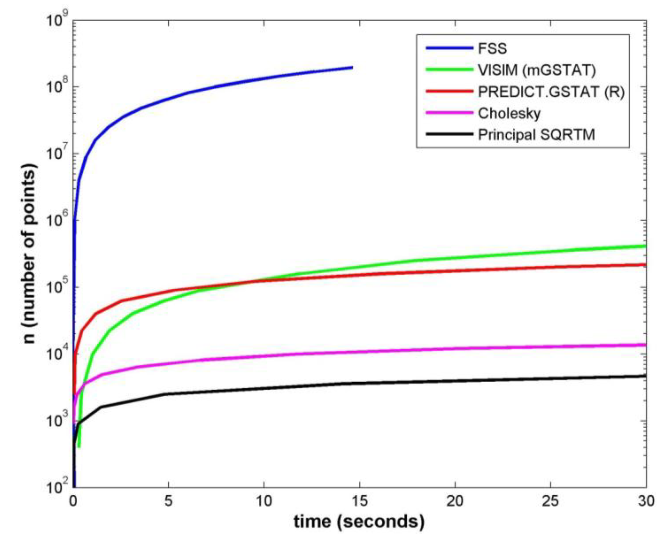
5.1. Timing Comparisons among Simulation Techniques
Figure 12 shows CPU time comparisons among five different techniques for simulating perturbations for a square grid by varying the number of points
n; where
![Ijgi 03 00817 i007]()
is the number of points along one side of the grid. Computation times were measured with a PC laptop with Intel i5 dual core 2.3 GHz CPUs and 8 GB of memory.
The objective was to measure the CPU performance of the main computation (sans overhead setup) for each method. Efforts were made to match the modeling parameters among all methods as closely as possible. Testing assumed unconditional, homogeneous, and isotropic models only (actually, for FSS the model was approximately isotropic, as
Tx =
Ty). The following describes what main computations were timed in each of the five methods, and are listed in ascending order of computational speed gain according to
Figure 12.
(1) Principal matrix square root (using Matlab function SQRTM)
where
![Ijgi 03 00817 i009]()
is the
nx
n principal matrix square root of
Σz;
r is a
n × 1 vector realization of
n independent
N(0,1) distributed random variables, and
ϵz is the
n × 1 vector of perturbations corresponding to the random variable
z or
z(
k, l) over the grid.
Σz was assumed to be a full, and positive definite matrix,
i.e., the
a priori covariance matrix corresponding to the random field at the
n different points in the grid. Matlab uses the Schur decomposition technique to compute SQRTM for a general square matrix, which can be further sped up for symmetric and real matrices.
Figure 12.
Time comparison among methods for unconditional simulation of a scalar random field z(k, l) over a 2D square grid (Note that FSS is cutoff at ~15 s due to reaching the system memory limit).
Figure 12.
Time comparison among methods for unconditional simulation of a scalar random field z(k, l) over a 2D square grid (Note that FSS is cutoff at ~15 s due to reaching the system memory limit).
(2) Cholesky decomposition (using Matlab function CHOL)
where
L is the lower triangular
nx
n matrix from the Cholesky decomposition,
Σz =
LL*, where
L* is the conjugate transpose of
L;
r is a
n × 1 vector realization of
n independent
N(0,1) distributed random variables, and
ϵz is the
n × 1 vector of perturbations corresponding to the random variable
z or
z(
k, l) over the grid.
Σz was assumed to be a full and positive definite matrix.
(3) PREDICT.GSTAT (version 1.0, 19 April 2014) [
10] is the algorithm based upon Pebesma [
11] as implemented and tested in the “R” (version 3.0.2, 64 bit) statistical package. The following R script is an example of parameters used to time unconditional simulation on a 100 × 100 grid. Note that only the execution of the PREDICT function was timed.
(4) VISIM in mGstat [
12] is a sequential simulation code based on GSLIB (Geostatistical Software LIBrary, Stanford Center for Reservoir Forecasting, Stanford University) [
13] for sequential Gaussian and direct sequential simulation. mGstat is a geostatistical Matlab toolbox available as open source that allows access to VISIM (among other algorithms) via a Matlab interface. The parameter file used to measure VISIM performance can be found in
Appendix C.
(5) Fast Sequential Simulation (FSS) is the technique described in this paper, and was coded and timed as a Matlab function. The main required parameters used were grid spacing (
δ = 1), standard deviation for the random variable (
σz = 1), and the spatial distance correlation constants (
Tx =
Ty= 10), as all described in
Section 2.3 and
Section 2.4 of this paper.
5.2. Discussion of Timing Results
The principal matrix square root (SQRTM) and Cholesky decomposition (CHOL) methods were provided to serve as a starting benchmark. While they are the least practical for large
n, their main benefit is providing an exact solution for any spatial distribution of points and any
a priori spatial statistics (valid covariance matrix).
Figure 12 shows Cholesky providing roughly half an order of magnitude speed gain over SQRTM.
PREDICT.GSTAT and VISIM provide implementations of standard geostatistical techniques for Sequential Gaussian Simulation.
Figure 12 shows that they provide comparable speed performance, and are 1–2 orders of magnitude faster than SQRTM and Cholesky. Their main advantage is providing broad flexibility for general purpose modeling among conditional and unconditional simulations. Moreover, additional speed efficiencies can be achieved when simulating multiple realizations with a fixed parameter set, which is not captured in
Figure 12. E.g., following a single random path through the locations, PREDICT.GSTAT reuses results for each of the subsequent simulations [
10].
FSS is the technique proposed in this paper. The two main advantages of FSS are (1) speed gain, e.g., three orders of magnitude faster than the next fastest technique as shown in
Figure 12; and (2) simplicity of operation, e.g., requiring only three main parameters. Note that the FSS curve in
Figure 12 is cutoff at ~15 s, which was due to reaching the memory limit for the grid size (
n > 2 × 10
8 points). However, this constraint can be easily overcome by performing the computation with a local moving window
versus storing the entire grid into system memory. The speed gain of FSS makes simulation of considerably denser grids more practical compared to the other methods. With this capability, our conjecture is that for those applications requiring interpolation, less expensive bilinear or nearest neighbor interpolation could be adequate for very dense grids
versus more expensive Kriging in coarser grids. The variogram (correlation) model is constrained to an exponential function with FSS, which makes it less flexible than the GSTAT (Sequential Gaussian Simulation) methods. However, the tradeoff in speed gain and simplicity of implementation offers practical and useful advantages to motivate a potentially broader community of users.
6. Extension of FSS to a Multivariate Gaussian 2D Random Field
The FSS core grid generation equation, Equation (3), can be extended from a scalar error
z to a (multivariate)
n × 1 error vector
X over a 2D grid in a straightforward manner. The more general case is presented directly below, with special but practical subcases presented in following subsections that include simpler notation.
where diagonal
![Ijgi 03 00817 i010]()
, 0 <
ri < 1,
i = 1,..,
n; diagonal
![Ijgi 03 00817 i011]()
, 0 <
si < 1,
i = 1,..,
n;
E{X(k, l) X(k, l)T = PX, the n × n covariance matrix;
E{X(k, l)X(k + ∆k, l + ∆l)T} = PX S∆k R∆l, {X(k, l)X(k ∆ ∆k, l + ∆l)T} = S∆k PX R∆l,
E{
X(
k,
l)
X(
k +
∆k,
l −
∆l)
T} =
R∆l PX S∆k,
E{
X(
k,
l)
X(
k −
∆k,
l −
∆l)
T} =
S∆k R∆lPX, for
∆k ≥ 0 and
∆l ≥ 0;
and
PU =
E{
U(
k,
l)
U(
k,
l)
T must be a valid (symmetric and positive definite) covariance matrix which satisfies the following:
PU = H * PX, the Hadamard product (term by term product) of two nxn matrices, where
![Ijgi 03 00817 i013]()
and
i,
j correspond to matrix row
i, column
j.
Note that the above constraint that PU is a positive definite matrix is not satisfied for all possible combinations of si, ri, and desired (valid) steady state error covariance PX, in which case Equation (9) and its statistics are no longer valid.
The corresponding derivation of the
a priori statistics for the above multivariate homogeneous Gaussian 2D random field, including the constraint for
PU, is somewhat complicated and presented in
Appendix D.
The actual grid generation algorithm associated with Equation (9) is as described previously in
Section 2.3 of this paper associated with Equation (3), except that
random_
N(0,
σz) is replaced by
![Ijgi 03 00817 i014]()
, and
random_
N(0,
σu) is replaced by
![Ijgi 03 00817 i015]()
, where the superscript 1/2 corresponds to principal matrix square root and
random_
v is the realization of an independent
nx1 random vector with each component an independent realization of a scalar random variable that is distributed
N(0,1). Of course,
S replaces
s,
R replaces
r , and
X replaces
z, as well.
Finally, for reasons similar to those presented in
Section 3.1 for the scalar random field, the above errors
X(
k,
l) are multivariate Gaussian distributed and correspond to a homogeneous random field. Again, see Reference [
1].
6.1. Common Spatial Correlation Subcase
The following is a special, but practical, subcase of Equation (9) where the constraint on
PU is always satisfied:
Where
R =
rInxn,
S =
sInxn,
PU = (1 −
s2)(1 −
r2)
PX.
This, in turn, leads to a simple form for the cross covariance and corresponding spatial spdcf: E{X(k, l)X(k + or − ∆k, l + or − ∆l)T } = ρ(∆k, ∆l)PX; that is, all n components of X(k, l) have common inter-grid (spatial) correlation via a common (scalar) spdcf ρ(∆k, ∆l) = s∆kr∆l = e−∆kδy/Tye−∆lδx/Tx
Note that Equation (10) allows for a full nxn covariance matrix PX, i.e., there can be non-zero intra-component correlations among the components of X(k, l). For example, assume that n = 3 and XT = [x y z] consists of error components x, y, and z. Furthermore, at an arbitrary grid point location (k, l) the z-component of error is correlated +0.10 with the y-component of error and the same x -component of error is correlated −0.60 with the z-component of error. Of course, all n-choose-2 (a value of 3 for the case n = 3) combinations of correlation among error components must correspond to a symmetric and positive definite PX.
Multi-Grid Point Covariance Matrix
For the special case of common spatial correlation, the corresponding
mn ×
mn multi-grid point covariance matrix for a collection of
X(
k,
l) at
m arbitrary grid points (
k,
l) has a convenient and valid representation:
Where Λ is an
mn × 1 vector such that
![Ijgi 03 00817 i017]()
and the
Xi =
X(
ki,
li),
i = 1,...,
m, correspond to an ordered list of the
m grid point locations. The
n ×
n cross-covariance terms
ρ(
∆yij, ∆xij)
PX consist of each element of
PX multiplied by the scalar value
ρ(
∆yij, ∆xij),
i,j = 1,...,
m.
6.2. Diagonal Covariance Subcase
Another special, but practical, subcase of Equation (9) is when the specified PX is a diagonal matrix. This allows for any values of 0 < si < 1 and 0 < ri < 1, i.e., different specifiable spatial correlations for each of the two directions for each of the n error components. Additionally, of course, this allows for different variances specified along the diagonal elements of PX; also, the constraint on PU is always satisfied. Note that this special case is simply equivalent to the scalar case for each of the n components applied independently.
The resultant system of equations are identical to Equation (9) except that we have the following diagonal matrices:
where
![Ijgi 03 00817 i019]()
Note that each component of X(k, l) has its own spatial correlation function with specifiable distance constants.
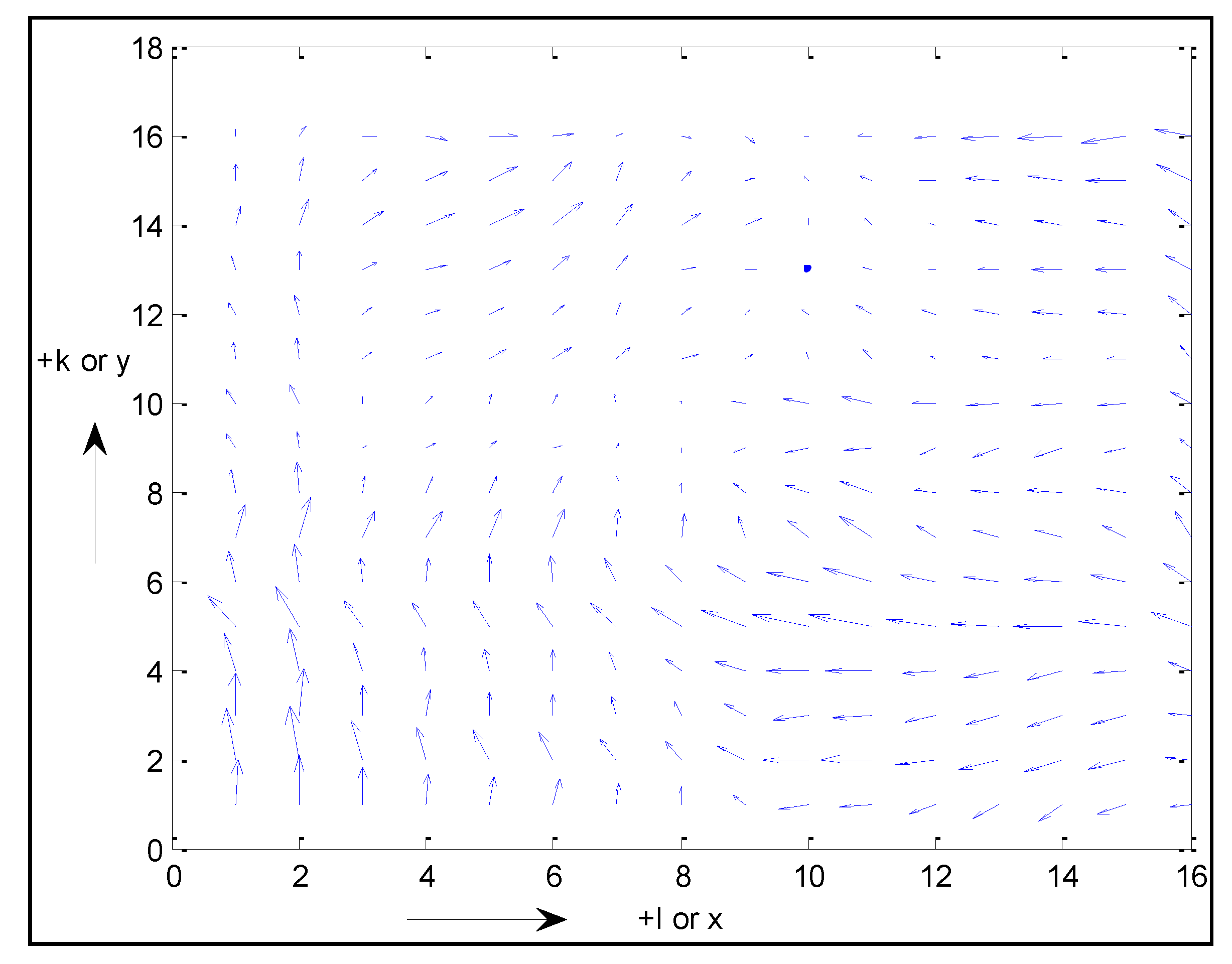
6.2.1. Example Realizations
This section presents quiver plots of multivariate error over a subset of a 2D final grid generated using the sequential algorithm discussed in
Section 6. The multivariate error corresponds to a two-dimensional vector (
n = 2). The corresponding covariance matrix is diagonal with a common variance for the two components of error for convenience,
i.e.,
![Ijgi 03 00817 i020]()
. Similarly, spatial correlations corresponding to a specific spatial direction are common for convenience,
i.e.,
s1 =
s2 and
r1 =
r2.
Figure 13 (automatically scaled) corresponds to
σ1 =
σ2 = 10 m, and
s1 =
s2 = 0.95 and
r1 =
r2 = 0.95.
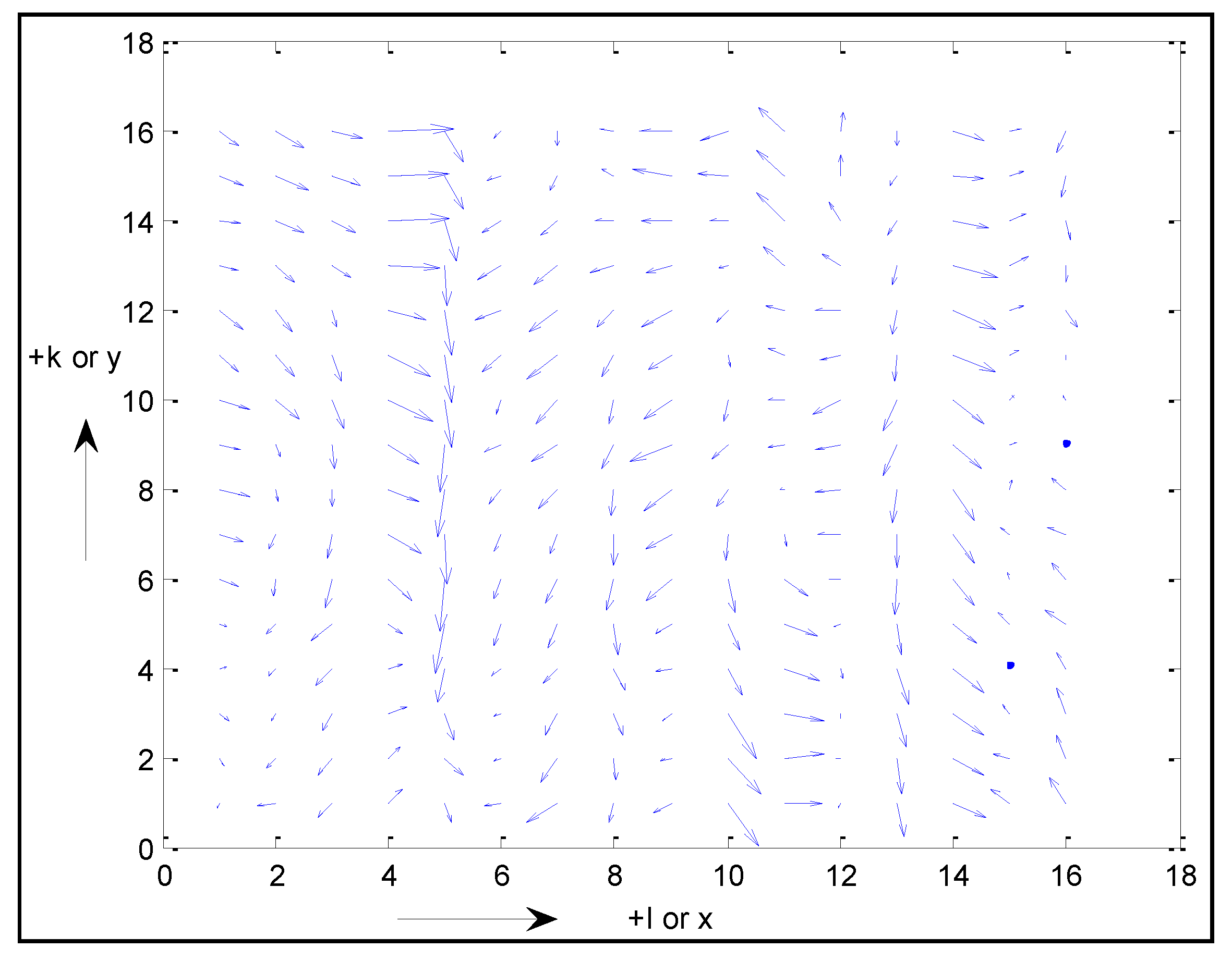
Figure 14 (automatically scaled) corresponds to
σ1 =
σ2 = 10 m, and
s1 =
s2 = 0.95 and
r1 =
r2 = 0. 5.
6.2.2. Multi-Grid Point Covariance Matrix
For the special case of a diagonal covariance matrix
PX, the corresponding
mn ×
mn covariance matrix for a collection of
X(
k,
l) at
m arbitrary grid points (
k,
l) has a convenient and valid representation:
where Λ is an
mnx1 vector such that
![Ijgi 03 00817 i017]()
and the
Xi =
X(
ki,
li),
i = 1,...,
m, correspond to an ordered list of the
m grid point locations. Also, * corresponds to the matrix Hadamard (element by element) product, the
nxn diagonal matrix
![Ijgi 03 00817 i022]()
, and
ρv(
∆yij, ∆xij) corresponds to the spatial correlation function associated with component
v = 1,...,
m of
X(
k,
l).
6.3. General Case with Constraint Enforced
Referring back to the general case of
Section 6, the following presents two examples for
n = 2. Assume that the two components of error correspond to
x-error and
y-error for specificity. From Equation (9),
s1, s2, r1, r2 can have any combination of values such that each is within the positive interval (0,1) and
PU, a function of the desired
PX and the
s1, s2, r1, r2, is a symmetric and positive definite matrix.
Figure 13.
Realization of two-dimensional multivariate errors over a 2D grid: high spatial correlation in the grid’s k or y-direction and high spatial correlation in the grid’s l or x-direction.
Figure 13.
Realization of two-dimensional multivariate errors over a 2D grid: high spatial correlation in the grid’s k or y-direction and high spatial correlation in the grid’s l or x-direction.
Subcase 1: Assume that
s1 =
s2 =
s and
r1 =
r2 =
r, to narrow down the possible combinations; therefore,
which is always positive definite for any
s and
r.
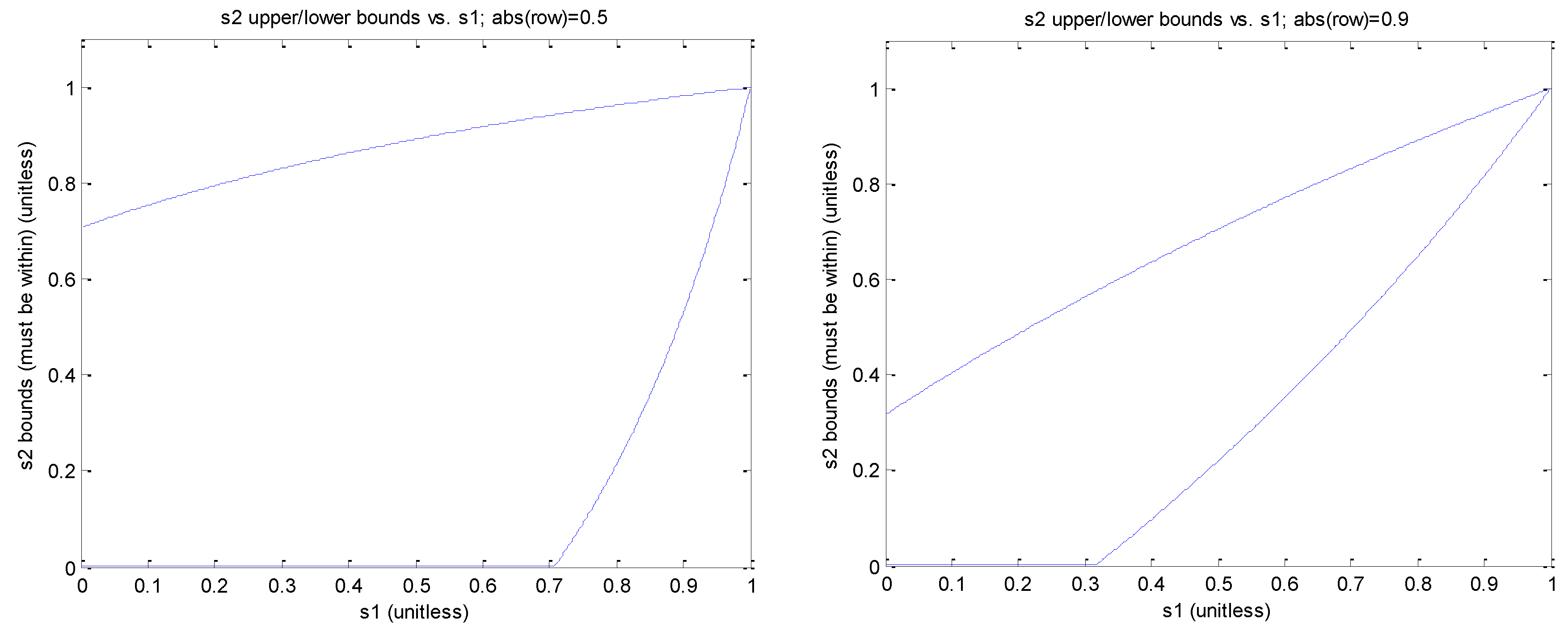
Subcase 2: Assume that
s1 =
r1 and
s2 =
r2, therefore,
which is positive definite if
The left portion of
Figure 15 plots the upper and lower bounds for
s2 given the desired value of
s1 and assuming that |
ρ| = 0.5; the right side assuming that |
ρ| = 0.9.
Figure 14.
Realization of two-dimensional multivariate errors over a 2D grid: high spatial correlation in the grid’s k or y-direction and lower spatial correlation in the grid’s l or x-direction.
Figure 14.
Realization of two-dimensional multivariate errors over a 2D grid: high spatial correlation in the grid’s k or y-direction and lower spatial correlation in the grid’s l or x-direction.
Figure 15.
Flow-down of constraints to spatial correlation bounds.
Figure 15.
Flow-down of constraints to spatial correlation bounds.
As can be seen from the above, the larger the absolute value of the correlation ρ between the error components x and y, the closer s2 = r2 must be to s1 = r1.
Note that any multi-grid point covariance matrix for this general case must be assembled “term-by-term” using the a priori statistics presented in Equation (9), i.e., there is no convenient functional form for the cross-covariances in the multi-grid point covariance matrix similar to those presented for the special case of common spatial correlation among the components of X(k, l) and the special case of a diagonal covariance matrix PX presented earlier.
7. Extension of FSS to a Non-Homogeneous 2D Random Field
This section of the paper extends the FSS of a scalar homogeneous Gaussian 2D random field to a scalar non-homogeneous Gaussian 2D random field. In particular, the specified values for σz, s, and r (variance and spatial correlation parameters) corresponding to z(k, l) are either explicitly or implicitly a function of grid location (k, l). There is no one “right way” to do the extension.
Two general methods are presented below, each practical but with different characteristics regarding the form of non-homogeneity represented. Each method can also compute a corresponding multi-grid point covariance matrix, necessary for many applications as discussed earlier in
Section 3. For one method, this covariance matrix is exact, for the other, an approximation. The best technique, when both non-homogeneity characteristics and possible multi-grid point covariance matrix approximations are taken into account, is application dependent. (The methods presented below can also be extended in a straightforward manner to multivariate non-homogeneous Gaussian 2D random fields.)
7.1. Method 1: Convex Combination
The core grid generation equation and corresponding sequential algorithm for scalar errors (
Section 2.2 and
Section 2.3) is simply exercised
n different times, either sequentially with the results saved temporally, or in parallel in order to save storage. (Of course, the grid size and spacing remains constant each time.) The number of times is typically two,
i.e.,
n = 2. Each uses a different set of specified
σz,
s, and
r. Thus, after the above is performed there are
n grids, each homogenous and in accordance with the
σz,
s , and
r specified for use with that particular grid. Each grid is uncorrelated with the others.
The
n grids of
z(
k,
l), designated
zi(
k,
l) for
i = 1,...,
n, are then combined based on a convex combination into a final grid of
z(
k,
l). That is, at each (
k,
l) location in the
p ×
q grid:
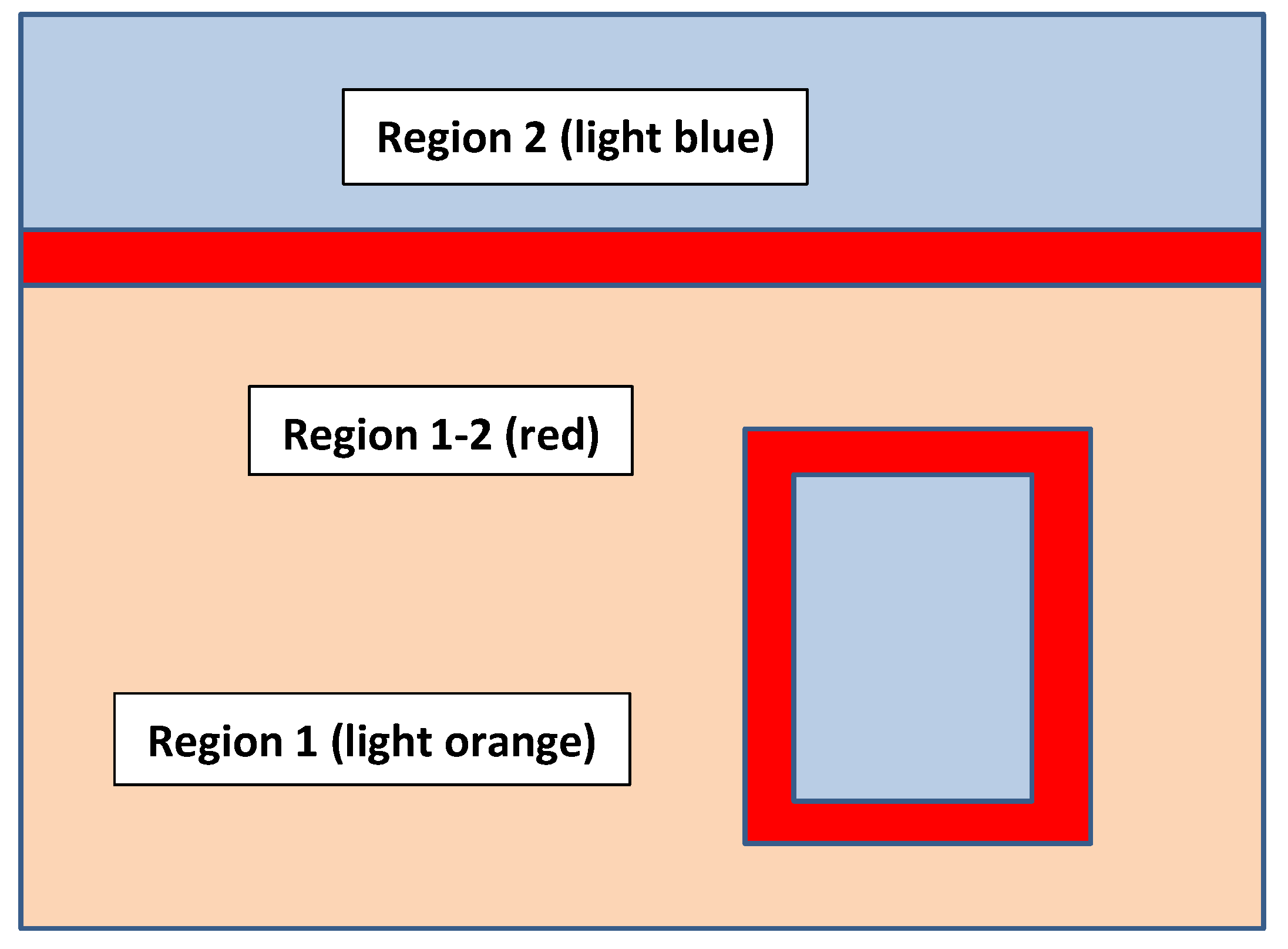
The specification of the wi(k, l) values, also symbolized as wikl for convenience, can be as simple or as complicated as appropriate over the locations across the p × q grid. However, their recommended values are in accordance with the following:
Let us assume that
z(
k,
l) is to be exclusively the value
zi(
k,
l) across the various (
k,
l) in
Region i of the
pxq grid; hence, in this region, all
wikl = 1. In addition, let us define
Region i–j as a “buffer region” from
Region i into
Region j. In this buffer region,
wikl varies linearly from 1–0 corresponding to the (
k,
l) at the start to the end of the buffer region, respectively. Furthermore, of course,
wjkl = 1 −
wikl throughout
Region i–j. Finally,
wikl = 0 for all locations (
k,
l) in
Region j. See
Figure 16 as an example for
n = 2.
Note that the width of the buffer region Region i–j should be at least twice the maximum of the corresponding spatial distance constants associated with zi(k, l) and zj(k, l), expressed in grid unit. This ensures reasonable spatial correlation across the buffer region. If there were no buffer region, the spatial correlation between two points, one anywhere in Region i and the other anywhere in Region j, would be 0, i.e., there would be an unwanted abrupt change across the boundary of the two regions.
Figure 16.
Example of region layout over a p × q grid.
Figure 16.
Example of region layout over a p × q grid.
7.1.1. Multi-Grid Point Covariance Matrix
Assume that
m different scalar
z(
k,
l) in the (final) grid are of interest regarding a corresponding multi-grid point covariance matrix. Each of these
z(
k,
l) corresponds to their own unique (
k,
l) location in the grid, and are ordered in a known fashion sequentially for
j = 1,...,
m, and placed into an
mx1 vector
Z, where
ZT = [
z1 …
zm]. Such a vector can also be defined for the same ordered locations for each of the different realizations as
Zi, = 1,...,
n. Therefore, based on Equation (17) we have:
where
Wi is an
mxm diagonal matrix for
i = 1,...,
n with the appropriate values of
![Ijgi 03 00817 i028]()
down its diagonal.
For example, if the first component of
Z corresponds to grid location (
k,
l) = (10, 20), the first diagonal component of
Wi equals
![Ijgi 03 00817 i029]()
.
Let us represent the corresponding
mxm multi grid point covariance matrix for the
Zi as
Pi. (See
Section 3 for how this matrix is computed given the corresponding
σz,
s, and
r.) The
mxm multi grid point covariance matrix for
Z is computed as follows:
A nice feature of Method 1 is that the above representation for the multi-grid point covariance matrix
P is exact.
P also corresponds to the following:
where
Z is an
mx1 vector such that
ZT = [
z1 …
zm] and the
zi =
z(
ki,
li),
i = 1,...,
m, correspond to the ordered list of the
m grid point locations;
ρj1j2 corresponds to the explicit correlation between two such points; the matrix entries “_” indicate symmetry.
7.1.2. Typical Statistics
The a priori statistics for a point and a point pair in the final z(k, l) grid are readily determined by the appropriate entries of a multi-grid point covariance matrix in which the two points are referenced. For convenience, results are summarized for a typical case as follows:
Assume a total of two regions and the typical values for w1kl in Region 1 (w1kl = 1), in Region 2 (w1kl = 0), and w1kl in Region 1–2 (w1kl = 1 → 0). Let us designate the a priori one-sigma and correlation functions for the homogeneous z1(k, l) and z2(k, l) across the grid as σz1 and ρ1(∆k, ∆l), and σz2 and ρ2(∆k, ∆l), respectively, for convenience. We have the following location-dependent statistics for the final combined z(k, l):
One-sigma value
σz: a point in Region 1,
σz1; a point in Region 2,
σz2; a point in Region 1–2,
![Ijgi 03 00817 i032]()
.
Spatial correlation function
ρ(
∆k, ∆l) value for a pair of points: both in Region 1,
ρ1(
∆k, ∆l); both in Region 2,
ρ2(
∆k, ∆l), one in Region 1 and one in Region 2, 0; one in Region 1 and one in Region 1–2,
![Ijgi 03 00817 i033]()
,
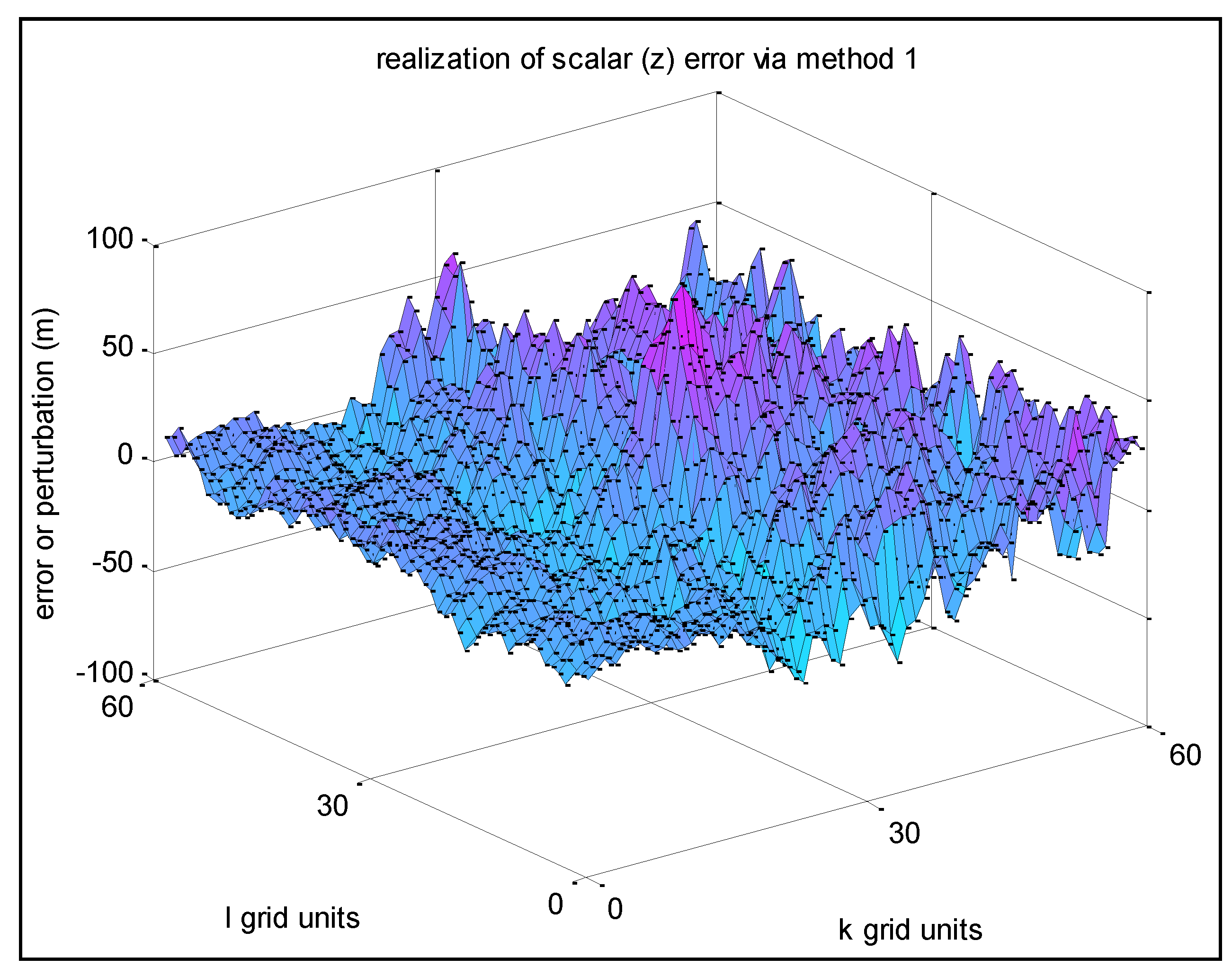
etc. 7.1.3. Example Realizations
The following non-homogeneous realization combines two homogeneous realizations with {
r1 =
s1 = 0.9,
σz1 = 10 m} and {
r2 =
s2 = 0.9,
σz2 = 30 m}, respectively.
Region 1 of the displayed portion of the final grid consists of
k = 1–10,
Region 1–2 k = 11–30, and
Region 2 k = 31–60. (For each region, the corresponding
l = 1–60.) Use of the typical assignment scheme for the values of
w1
kl (and
w2
kl = 1 −
w1
kl) was employed.
Figure 17 below presents the results.
Figure 17.
A smooth transition from Region 1 to Region 2, each with their own specified a priori statistics.
Figure 17.
A smooth transition from Region 1 to Region 2, each with their own specified a priori statistics.
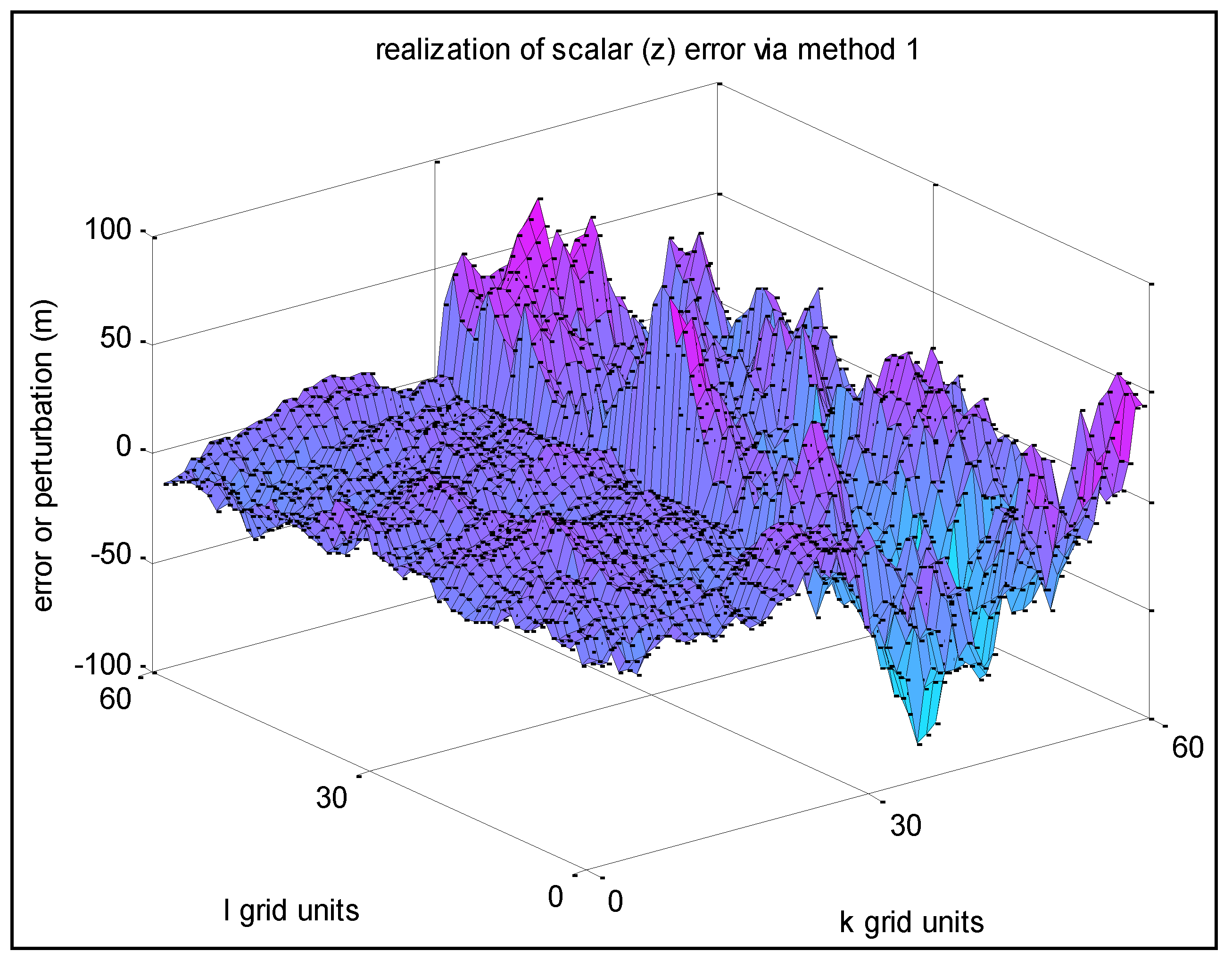
The same experiment was performed (but different realization) except that there was no
Region 1–2,
i.e., a non-typical scheme.
Figure 18 below presents the results.
7.2. Method 2: Functional Variation of a Priori Statistics
With the second method, the core grid generation equation and corresponding sequential algorithm for scalar errors (
Section 2.2 and
Section 2.3) is implemented only once, but modified as follows:
where
u(
k,
l) is a random sample of Gaussian white noise distributed
N(0, σ
u (
k,
l)), and where
![Ijgi 03 00817 i034]()
. Also,
s(
k,
l) =
e−δy/Ty(k,l), and
r(
k,
l) =
e−δx/Tx(k,l), that is, the spatial distance constants can be considered a function of (
k,
l) as well.
Figure 18.
An abrupt transition between Region 1 and Region 2, each with their own specified a priori statistics.
Figure 18.
An abrupt transition between Region 1 and Region 2, each with their own specified a priori statistics.
As indicated above, the values for σ
z,
s, and
r, and hence σ
u, are a function of the grid location (
k,
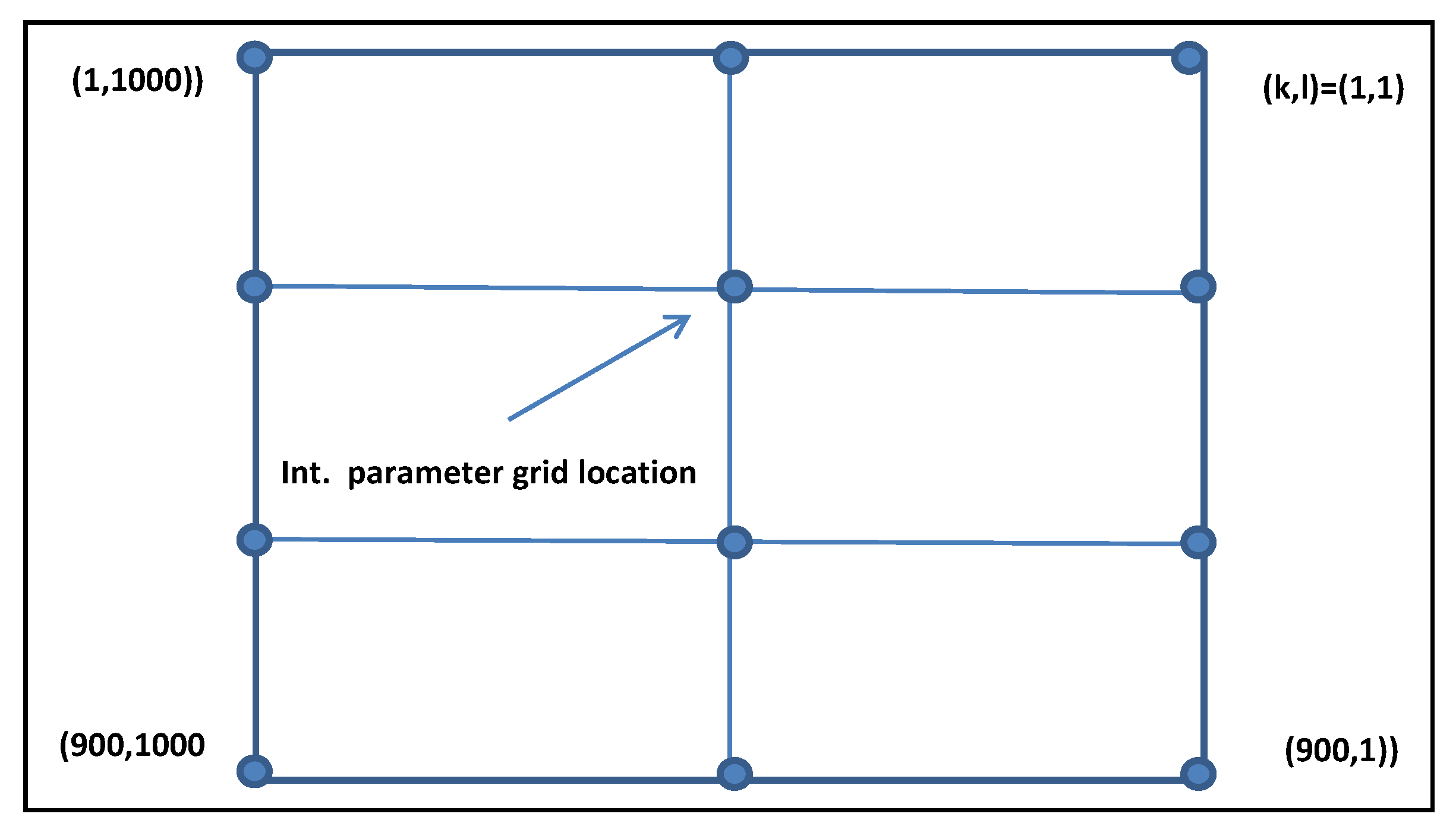
l). In addition, for Method 2, they are determined by the bilinear interpolation of such specified values over a less-dense grid overlaying the grid of errors to be generated. For example, if the 2D
pxq grid of errors to be generated is 900 × 1000, the grid for interpolation might be an evenly spaced 4 × 3 parameter grid overlying the denser grid. Each of the corresponding 12 parameter grid points contains the specified values for σ
z,
s , and
r for the corresponding local region around the parameter grid point. Note that σ
u is a function of the interpolated values of σ
z,
s, and
r; hence, is also recalculated in Equation (21) for every grid location (
k,
l). See
Figure 19 for a graphical representation of the interpolation parameter grid. Each interpolation parameter grid location contains a unique set of values for σ
z,
s, and
r.
Also, the spacing between interpolation parameter grid points should be at least twice the maximum of the corresponding spatial distance constants associated with that grid point and the other interpolation parameter grid points immediately surrounding it, expressed in grid unit. This ensures that both the desired and the computed approximation of the
a priori statistics corresponding to the
z(
k,
l) across the dense grid are approximately met and reasonably reliable (see
Section 7.2.2), respectively. (This also assumes that the appropriate buffer relative to the “final” grid is included as well—see
Section 2.3.2)
Once defined appropriately, Equation (21) is then implemented via a direct counterpart to the algorithm described in
Section 2.3. The latter simply utilizes the appropriate
σu,
s, and
r values that vary with (
k,
l) location.
Figure 19.
An example of an Interpolation Parameter Grid.
Figure 19.
An example of an Interpolation Parameter Grid.
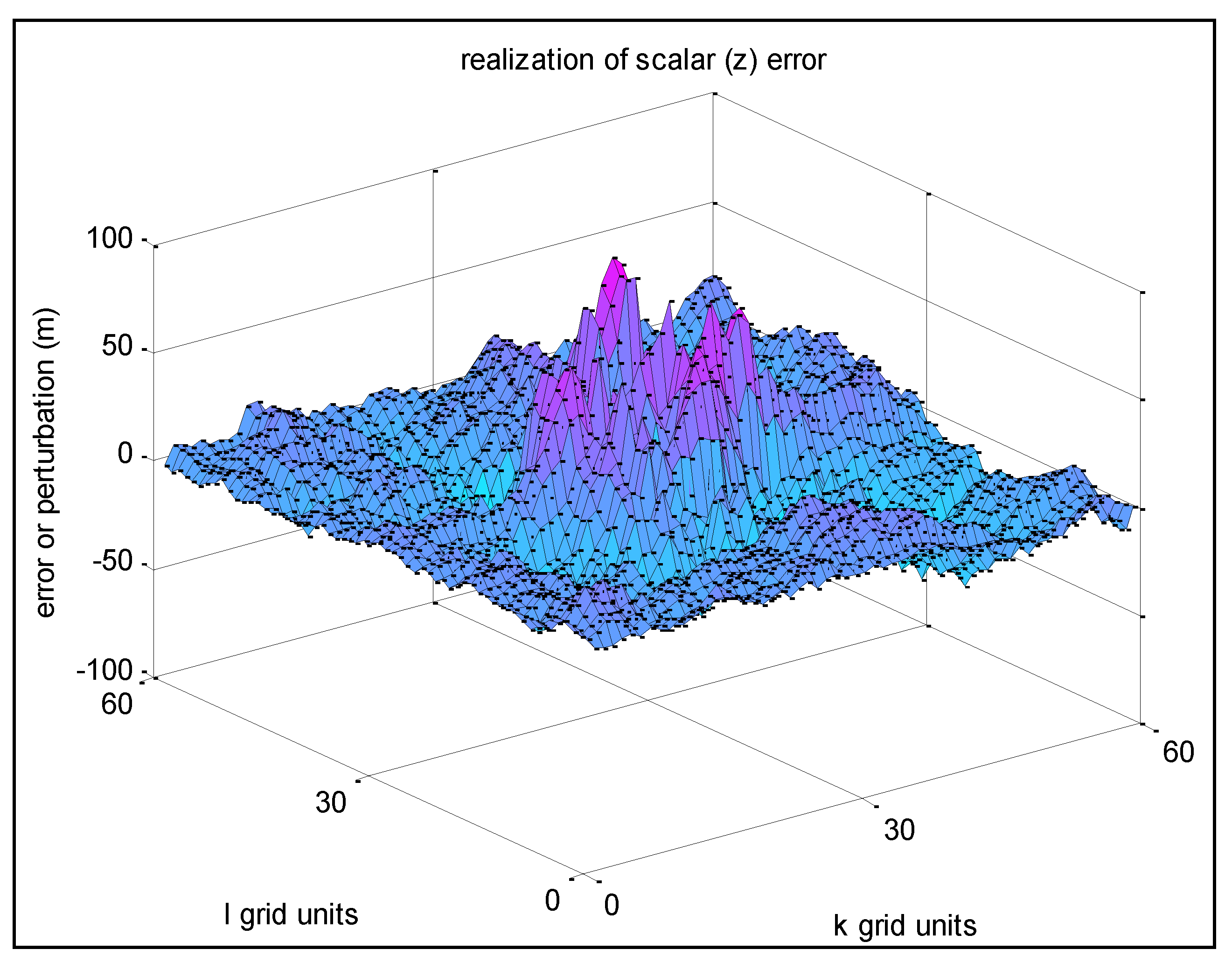
7.2.1. Example Realizations
The following examples correspond to a 7 × 7 parameter interpolation grid overlaying a 90 × 90 2D grid. The results corresponding to a 60 × 60 displayed portion of the final grid are presented.
All 49 sets of {
s,r,σz} parameters were identical except for four sets corresponding to an interior rectangle near the center of the final grid. Let us term the 45 common sets as Group 1 and the other four common sets as Group 2. In
Figure 20 below, the Group 1 set contain values
σz = 10 m,
s =
r = 0.9. Group 2 sets contain values
σz = 50 m,
s =
r = 0.9.
In
Figure 21 below, the Group 1 sets contain
σz = 10 m,
s =
r = 0.1. Group 2 sets contain
σz = 50 m,
r = 0.95
7.2.2. Statistics and Multi-Grid Point Covariance Matrix
Corresponding
a priori statistics are no longer straightforward for this method, but can be approximated. In particular,
σz corresponding to a specific location (
k,
l) is the corresponding bilinear interpolated value. The spatial correlation function corresponding to
m different locations (
k,
l) is the average of
m spatial correlation functions, each corresponding to the bilinear interpolated values for and
r for that location. Of course, these statistics reflect non-homogeneity,
i.e., are a function of the specific (
k,
l) locations of interest. The corresponding
mxm approximation for the multi-grid point covariance matrix corresponding to scalar errors at
m different grid locations is represented as follows:
where
Z is an
mx1 vector such that
ZT = [
z1 ...
zm] and the
zi =
z(
ki,
li),
i = 1,...,
m, correspond to an ordered list of the
m grid point locations.
Figure 20.
Non-homogeneous scalar realization—different variances.
Figure 20.
Non-homogeneous scalar realization—different variances.
Figure 21.
Non-homogeneous scalar realization—different variances and spatial correlations.
Figure 21.
Non-homogeneous scalar realization—different variances and spatial correlations.
![Ijgi 03 00817 i036]()
, and the individual spatial correlation functions are defined by their corresponding interpolated values for
s and
r.
Because the average of a collection of strictly positive definite correlation functions (spdcfs) is an spdcf itself, the above is guaranteed a valid covariance matrix regardless of the fact that the various
σzi can vary in value (Reference [
7]).
Note that if the m grid points consist of widely spaced subgroups of points such that the scalar error at any grid point in one subgroup has (approximated) low correlation (e.g., less than 0.1) with the scalar error at any grid point in any other subgroup, a higher fidelity representation for the multi-grid point covariance matrix can be achieved as follows: Use the representation in Equation (22) to compute a “sub-multi-grid point covariance matrix” for each subgroup of grid points, and then combine them into the (final) multi-grid point covariance matrix by placing (in order) each sub-multi-grid point covariance matrix down the block diagonals with values of zero for all off-diagonal (cross-covariance) blocks.
Finally, to generate a multi-grid point covariance matrix for a non-homogeneous multivariate
X(
k,
l) instead of that for a non-homogeneous scalar
z(
k,
l), the same general procedure presented in this section can be extended in a straightforward manner using methods described in References [
6,
7].
8. Summary and Conclusions
Practical methods for the sequential generation of two-dimensional random fields were presented, and their corresponding multivariate covariance matrices derived. The corresponding methods were based on FSS, which was also compared to Sequential Gaussian Simulation and other approaches. Although less general, FSS was shown to be clearly superior in terms of speed and simplicity, primarily due to assumed separable exponential spatial correlation and simple ordered generation over an evenly spaced grid. FSS methods presented in the paper are applicable to performance assessment and tuning of geospatial applications in a simulation environment, as well as near-real time display of the effect of errors on applications by the applications themselves.


 . That is, given a desired s, r, and σz, a corresponding value of σu is computed per the above.

 and width of side buffer (# grid columns) = 2Tx/δx. Or equivalently, if s and r equal the value 0.9, 19 grid rows and 19 grid columns. This will ensure generation of errors throughout the final grid with the desired statistical properties.


 and have inter-grid point correlation between pairs corresponding to a normalized strictly positive definite correlation function (spdcf) ρ(∆k, ∆l) = ρ(∆y, ∆x) = e−∆lδy/Tye−∆kδx/Tx, i.e., the multi-grid point covariance matrix equals:


 is the number of points along one side of the grid. Computation times were measured with a PC laptop with Intel i5 dual core 2.3 GHz CPUs and 8 GB of memory.
 is the nxn principal matrix square root of Σz; r is a n × 1 vector realization of n independent N(0,1) distributed random variables, and ϵz is the n × 1 vector of perturbations corresponding to the random variable z or z(k, l) over the grid. Σz was assumed to be a full, and positive definite matrix, i.e., the a priori covariance matrix corresponding to the random field at the n different points in the grid. Matlab uses the Schur decomposition technique to compute SQRTM for a general square matrix, which can be further sped up for symmetric and real matrices.

 , 0 < ri < 1, i = 1,..,n; diagonal
  , 0 < si < 1, i = 1,..,n;
 and i, j correspond to matrix row i, column j.
 , and random_N(0, σu) is replaced by
  , where the superscript 1/2 corresponds to principal matrix square root and random_v is the realization of an independent nx1 random vector with each component an independent realization of a scalar random variable that is distributed N(0,1). Of course, S replaces s, R replaces r , and X replaces z, as well.
 and the Xi = X(ki, li), i = 1,...,m, correspond to an ordered list of the m grid point locations. The n × n cross-covariance terms ρ(∆yij, ∆xij)PX consist of each element of PX multiplied by the scalar value ρ(∆yij, ∆xij), i,j = 1,...,m.

 . Similarly, spatial correlations corresponding to a specific spatial direction are common for convenience, i.e., s1 = s2 and r1 = r2. Figure 13 (automatically scaled) corresponds to σ1 = σ2 = 10 m, and s1 = s2 = 0.95 and r1 = r2 = 0.95. Figure 14 (automatically scaled) corresponds to σ1 = σ2 = 10 m, and s1 = s2 = 0.95 and r1 = r2 = 0. 5.
 , and ρv(∆yij, ∆xij) corresponds to the spatial correlation function associated with component v = 1,...,m of X(k, l).


 down its diagonal.
  .
.

 .
. , etc.
 . Also, s(k, l) = e−δy/Ty(k,l), and r(k, l) = e−δx/Tx(k,l), that is, the spatial distance constants can be considered a function of (k, l) as well.


 , and the individual spatial correlation functions are defined by their corresponding interpolated values for s and r.


 or more generally, E{z(k, l)z(k + or − ∆k, l + or − ∆l)} =
  .
.
 , and E{u(k, l)u(p, q) } = 0 for p ≠ k or q ≠ l; by the properties of a geometric series,
  , where 0 < a < 1, which is applicable since 0 < a = s2 = e−2δy/Ty < 1 and 0 < a = r2 = e−2δx/Tx < 1 in the above.


 , i.e., the variance of the Kriging solution relative to the value of the true realization.
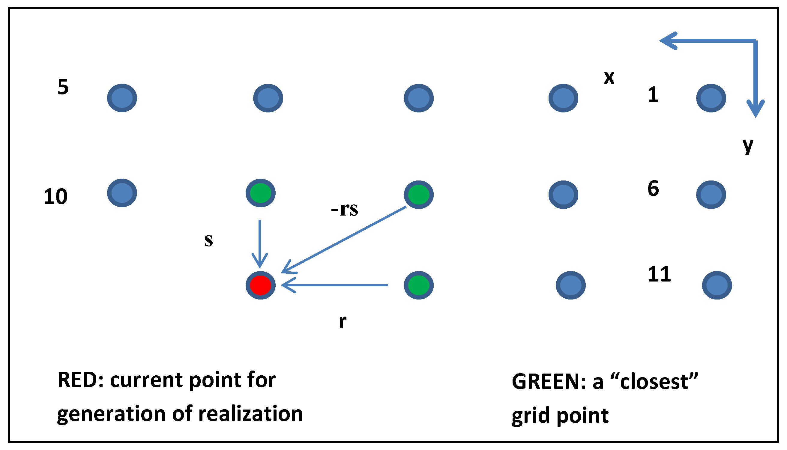
 [7.15 6.20 5.45 6.88 8.08 8.66 8.46 5.92 8.16 11.28 8.88 9.99 8.34] and X2 = [9.81]. (Components 1–13 of X1 correspond to grid points #1–13, and X2 corresponds to the red point in Figure B1.) During generation of X2, the additive Gaussian random number u per Equation (3) was equal to −0.39 corresponding to the standard deviation
  = 1.31. (Also. using the symbology of Equation (3), X2 corresponds to z(k + 1, l + 1) and u to u(k + 1, l + 1).)
 (1 × 13), and
  (13x13). Therefore, given the values of r and s specified earlier, P21P11−1 = [0 0 0 0 0 0 0 −rs s 0 0 0 r] = [0 0 0 0 0 0 0 −86 0.95 0 0 0 0.90], and the solution (with additive random number) is P21P11−1X1 − 0.39 = 9.81, identical to that generated using the FSS method of this paper. In addition, σX2 = 1.31, which is equal to σu. These equivalences and the use of only the nearest three grid points were enabled due to both the separable exponential spatial correlation and the regular grid of realizations generated in a simple, ordered fashion. (Thus, for example, if grid point #8 were moved +0.5 grid units in the y-direction, there would be 7 instead of 3 non-zero scalar weights.)
 , which is easily verified by direct evaluation of P21P11−1P12 = WP12.

 , p, q∈{1,…,v}.
 . Also, PU must be positive definite in order that PX is positive definite via the earlier summation. (Note that, in the above, SmRn = RnSm, i.e., they commute since they are diagonal matrices.) Also,
