Remote Sensing Image Fusion at the Segment Level Using a Spatially-Weighted Approach: Applications for Land Cover Spectral Analysis and Mapping

Abstract

Segment-level image fusion involves segmenting a higher spatial resolution (HSR) image to derive boundaries of land cover objects, and then extracting additional descriptors of image segments (polygons) from a lower spatial resolution (LSR) image. In past research, an unweighted segment-level fusion (USF) approach, which extracts information from a resampled LSR image, resulted in more accurate land cover classification than the use of HSR imagery alone. However, simply fusing the LSR image with segment polygons may lead to significant errors due to the high level of noise in pixels along the segment boundaries (i.e., pixels containing multiple land cover types). To mitigate this, a spatially-weighted segment-level fusion (SWSF) method was proposed for extracting descriptors (mean spectral values) of segments from LSR images. SWSF reduces the weights of LSR pixels located on or near segment boundaries to reduce errors in the fusion process. Compared to the USF approach, SWSF extracted more accurate spectral properties of land cover objects when the ratio of the LSR image resolution to the HSR image resolution was greater than 2:1, and SWSF was also shown to increase classification accuracy. SWSF can be used to fuse any type of imagery at the segment level since it is insensitive to spectral differences between the LSR and HSR images (e.g., different spectral ranges of the images or different image acquisition dates).

1. Introduction

Image segmentation has become a quite common pre-processing task in remote sensing. It involves sub-dividing an image into relatively homogeneous image regions (polygons) often referred to as “image segments” or “image objects” [1]. These image segments are then used for further image processing (e.g., object-based classification or regression tasks), either instead of [1,2,3,4,5] or in combination with [6,7,8] individual pixels. Descriptors of the pixels located within an image segment, such as the pixels’ reflectance values at different electromagnetic wavelengths, are typically used to derive several of the segment’s descriptors, such as its mean reflectance value at different electromagnetic wavelengths. Mean spectral values (e.g., radiance, reflectance, etc.) are probably the most commonly-used descriptors of image segments, although textural descriptors and geometric descriptors are also often used (e.g., [2,4,5,9]). In this study, the focus is on mean spectral values of image segments, derived from the pixels within each segment.

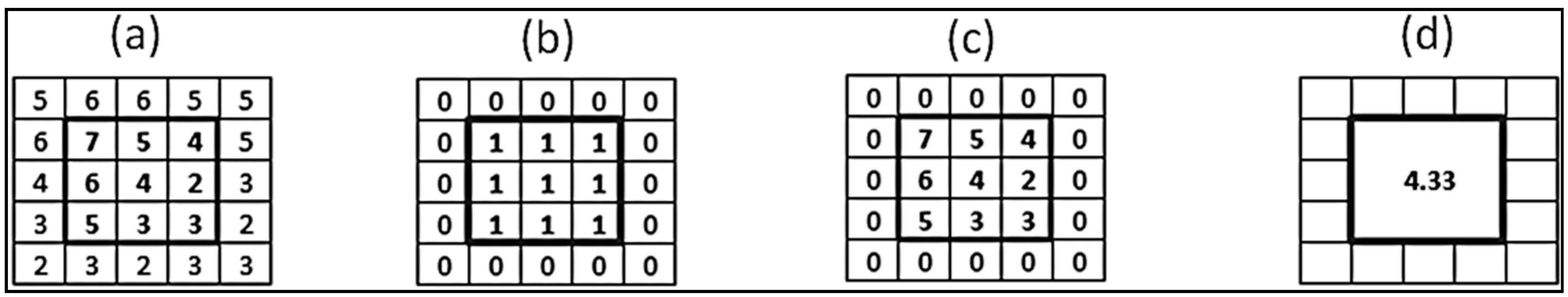
Existing methods for calculating mean spectral values involve assigning equal weights to all pixels within a segment, as shown in Figure 1. However, for various reasons, it may be preferable to derive the mean spectral values using a weighted calculation method rather than by simply weighting all pixels equally. 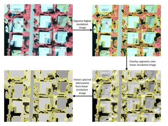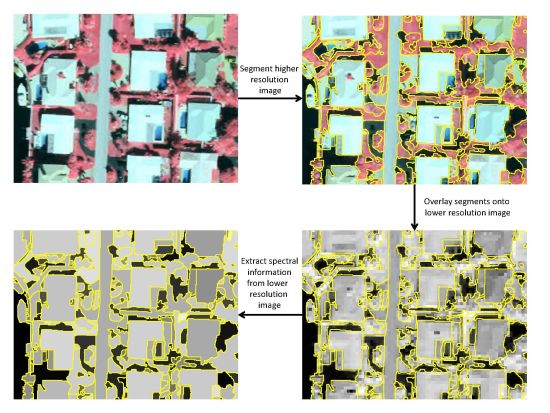For example, as shown in Figure 2, in some cases a segment may intersect one or more pixels, causing the pixels to be located only partially within the segment (i.e., “partial sub-objects” of the segment). This often occurs if a higher spatial resolution (HSR) image is segmented and then the segment polygons are overlaid onto a lower spatial resolution (LSR) image to derive additional descriptors of the segments, such as higher spectral resolution [10,11] or higher temporal resolution information. Compared to pixel-based image fusion, which is relatively common nowadays in remote sensing [12], few studies have investigated fusion at the segment (polygon) level [10,13,14]. Here, for simplicity this procedure is referred to as segment-level fusion (also referred to as pixel/feature-level fusion in [11]).

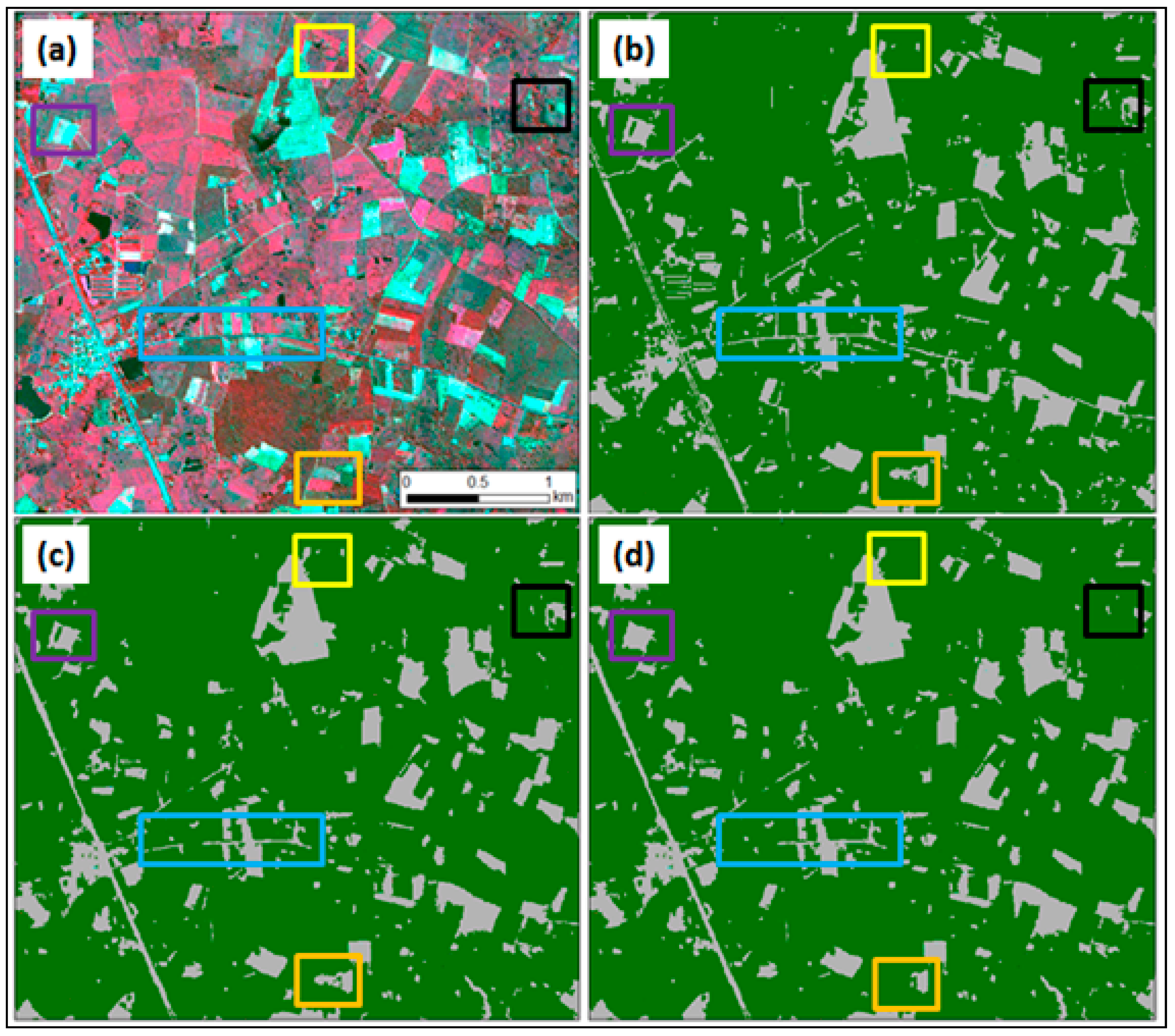
Figure 1. An image segment polygon (bold line) overlaid onto a grid of pixels with intensity values (a); the weights assigned to the pixels within the polygon (b); new values calculated by multiplying the pixel intensity values by their weights (c); the mean segment intensity value (d); calculated by dividing the sum of the values in (c) by the sum of the weights in (b).

Figure 1. An image segment polygon (bold line) overlaid onto a grid of pixels with intensity values (a); the weights assigned to the pixels within the polygon (b); new values calculated by multiplying the pixel intensity values by their weights (c); the mean segment intensity value (d); calculated by dividing the sum of the values in (c) by the sum of the weights in (b).

The most simple segment-level fusion approach is to resample the LSR image to match the HSR image that the segments were derived from, as shown in Figure 2, and then calculate the mean segment value from the resampled pixels. Here, this is referred to as the unweighted segment-level fusion (USF) approach, and it is implemented (or easy to implement) in commonly-used image segmentation software packages such as Trimble’s eCognition [15]. However, partial sub-objects are not ideal as segment descriptors because they are derived, in part, from locations outside of the segment they are describing. This makes them less accurate descriptors of the segment than pixels located completely within the segment at their original spatial resolution (i.e., the “true sub-objects” of the segment). In addition to these problems related to partial sub-objects, true sub-objects of a segment may also contain unwanted noise from nearby areas, particularly the true sub-objects located adjacent to segment boundaries. This noise can be caused by many factors, including diffuse electromagnetic reflection from nearby land cover objects, motion blur, and/or geo-location errors in one or more of the images. Thus in many cases the pixels located on or near a segment’s boundary will be less accurate descriptors of the segment than the pixels located at more interior locations within the segment. So, while previous studies on segment-level fusion have used the USF approach, it may be preferable to instead adjust the weights of pixels based on their distance from segment boundaries (i.e., reduce the weight of resampled pixels located near segment boundaries) for mean segment value calculations.

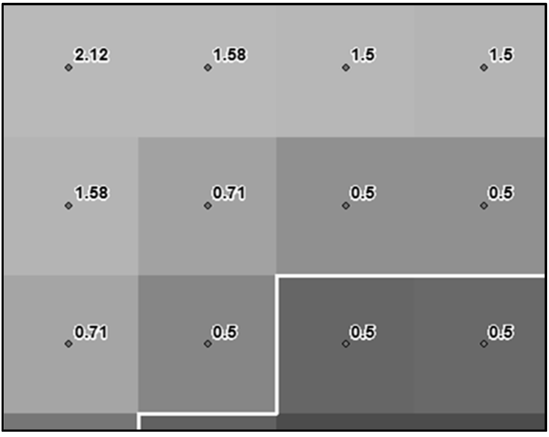
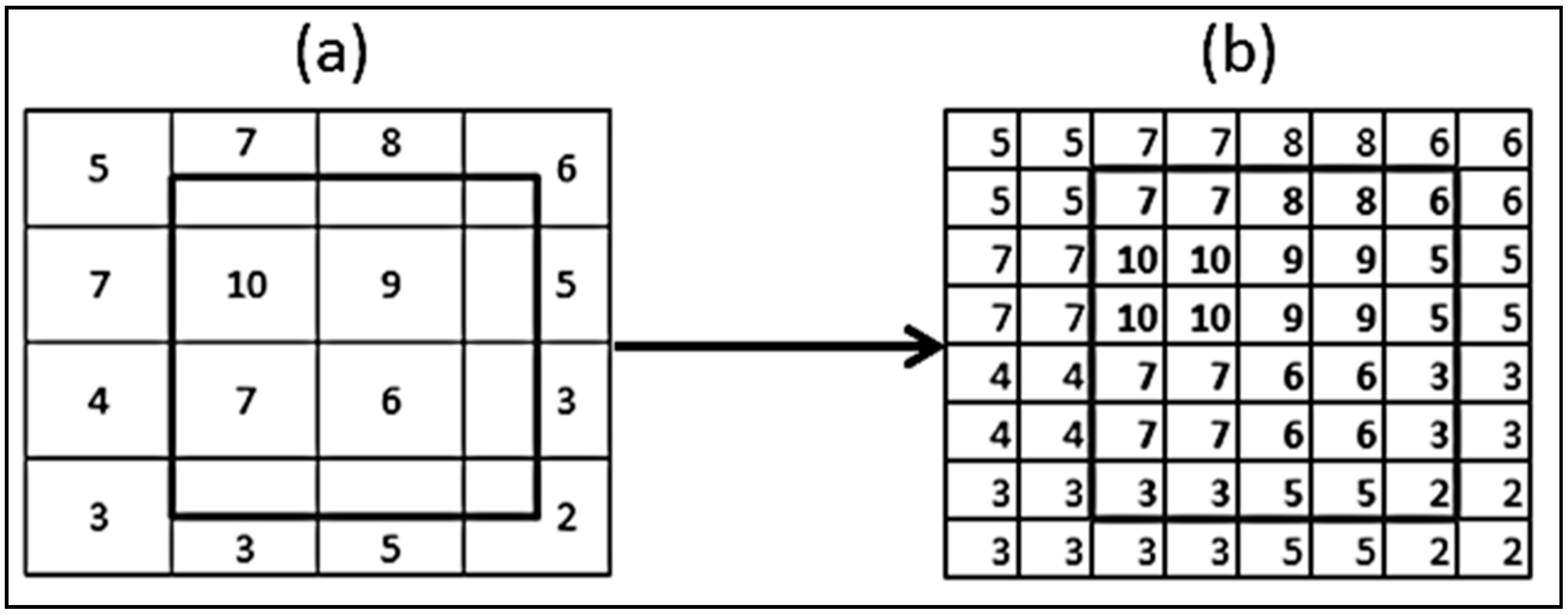
Figure 2. Image segment polygon (bold line) overlaid onto a grid of pixels with intensity values (a). The intersected pixels in (a) are the partial sub-objects of the segment, while the pixels located completely within the segment are the true sub-objects of the segment. The pixels from (a) are resampled to ½ of their original spatial resolution (e.g., from 30 m to 15 m resolution) using nearest neighbor resampling, and the intensity values of the resampled pixels are shown in (b).

Figure 2. Image segment polygon (bold line) overlaid onto a grid of pixels with intensity values (a). The intersected pixels in (a) are the partial sub-objects of the segment, while the pixels located completely within the segment are the true sub-objects of the segment. The pixels from (a) are resampled to ½ of their original spatial resolution (e.g., from 30 m to 15 m resolution) using nearest neighbor resampling, and the intensity values of the resampled pixels are shown in (b).

In this study, a spatially-weighted segment-level fusion (SWSF) approach is proposed to derive mean segment values from a LSR image. The proposed approach involves: (1) segmenting a HSR image; (2) resampling a LSR image to match the HSR image; (3) calculating a spatial weight for each resampled LSR pixel based on its Euclidean distance from the boundary of the segment it is located within; and (4) calculating the mean value of each segment based on the values of the resampled LSR pixels and their spatial weights. The proposed SWSF approach is compared with the traditional USF approach to determine which is more suitable for segment-level fusion of images with different spatial resolutions. We evaluated the performance of SWSF and USF using two case studies. The first involved extracting spectral values of urban land cover features in a very high (0.3 m) resolution image, and the second involved classifying a high (6.5 m) resolution image of a mixed agricultural/forested area.

2. Methods

2.1. Case Study 1: Urban Area

2.1.1. Study Area and Data

In the first case study, a 0.3 m resolution color infrared (CIR) aerial orthoimage of an urban area in Deerfield Beach, USA (26.28°N, 80.08°W) was used to demonstrate the performance of the proposed SWSF approach under several different scenarios (i.e., several different LSR:HSR image ratios). The objective of this case study was to evaluate whether USF or SWSF could extract more accurate spectral values of urban land cover features in these scenarios. The study area image was 500 × 500 pixels and contained a variety of urban land cover, including buildings, vehicles (cars and boats), pavements with different reflectance properties, mixed vegetation, pools, and a canal. Pixel values were in digital number (DN) units ranging from 0 to 255 (8-bit data).

A reference segmentation of the scene was obtained by manually digitizing the boundary of each land cover object in the image (415 polygons in total). The digitized vector polygons were rasterized to 0.3 m resolution to match the spatial resolution of the orthoimage. Often, automated methods, such as the multi-resolution segmentation algorithm [1] implemented in eCognition [15], are used for image segmentation, but manually-delineated polygons are also used, particularly when very high accuracy is desired (e.g., for delineating legal property boundaries, important vegetation types, etc.). The proposed SWSF method can be applied to segments generated by either automated or manual image segmentation. A manual segmentation was used in this first case study (while an automated segmentation was used in the second case study).

2.1.2. Extracting Mean Spectral Values of Segments from Simulated LSR Images

For segment-level fusion, ideally the segment descriptors extracted from a LSR image should be equivalent to the segment descriptors that would be extracted if the LSR image were acquired at the same spatial resolution as the HSR. For example, if a 30 m resolution Landsat image is segmented and additional segment values are extracted from a 250 m resolution MODIS image, the segment descriptors extracted from the MODIS image should ideally be equivalent to the segment descriptors that would be extracted from a 30 m resolution MODIS image. Since it is impossible to test this property using real data, in this study the HSR image was instead degraded to several coarser spatial resolutions to generate simulated LSR images, and the mean segment values extracted from the HSR image were compared with the values extracted from the LSR images. Cubic convolution resampling [16], implemented in ESRI ArcGIS 10, was used to generate the simulated LSR images, and then the LSR images were resampled back to 0.3 m resolution by nearest neighbor resampling to match the HSR image. LSR images were generated at two times (0.6 m), three times (0.9 m), five times (1.5 m), and ten times (3.0 m) the spatial resolution of the HSR image to evaluate performance at various relative image resolutions (2:1, 3:1, 5:1, 10:1). Only the near infrared (NIR) band was used for this analysis since it was shown to be the most useful band for discriminating land cover objects in a previous study of the area [17], but the results should be similar for all spectral bands since only the spatial resolution of the imagery was altered. Figure 3 shows the reference image segments overlaid onto the NIR band at four different spatial resolutions.

Figure 3. Reference image segments (white lines) overlaid onto the near infrared image of the study area at 0.3 m (a), 0.6 m (b), 1.5 m (c), and 3.0 m (d) spatial resolutions.

Figure 3. Reference image segments (white lines) overlaid onto the near infrared image of the study area at 0.3 m (a), 0.6 m (b), 1.5 m (c), and 3.0 m (d) spatial resolutions.

Since the objective in this experiment is to get the mean segment values extracted from the LSR image to closely match the mean values extracted from the HSR reference image, for SWSF to be effective it should produce values more similar to the HSR values than the USF approach. Mean Average Error (MAE) and Root Mean Square Error (RMSE) were both used to measure the differences between the mean segment values extracted from the HSR and LSR images.

2.1.3. Spatially-Weighted Segment-Level Fusion (SWSF)

As previously discussed, SWSF assigns spatial weights to the resampled (0.3 m) LSR pixels based on their Euclidean distance from segment boundaries. These spatial weights are then used to calculate the weighted mean (WM) value of each segment, given by:

$$WM= \frac{{{\displaystyle \sum }}_{i=1}^n(w_i{y}_i)}{{{\displaystyle \sum }}_{i=1}^n{w}_i}$$

(1)

where n is the number of pixels within the segment, w_i is the spatial weight of pixel i, and y_i is the pixel value of pixel i.

For illustration simplicity, the distances were calculated, in pixel units, from the center of a pixel to the nearest polygon boundary, as shown in Figure 4. Nine different weighting schemes were tested for deriving spatial weights from these distance measurements, as the most effective weighting scheme may vary based on the spatial resolution of LSR image relative to that of the HSR image. In all nine weighting schemes, spatial weights increase linearly until a certain distance threshold is reached, after which they stop increasing. Assigning spatial weights of 0 to any pixels could cause some image segments to have WM values of 0 (e.g., if a segment consists of only partial sub-objects, which is not unusual), so all pixels have weights > 0 in the nine weighting schemes. For the first weighting scheme, W1, the spatial weights increase linearly until a distance of one pixel unit (i.e., 0.3 m) from the segment boundary is reached, as shown in Figure 5a. So, in this weighting scheme, only the pixels vertically, horizontally, or diagonally adjacent to segment boundaries are penalized with lower weights (i.e., weights < 1). The other eight weighting schemes—W2–W9—are calculated similarly to W1, but with different distance thresholds. As shown in Figure 5, for W2, W3, and W4, the spatial weights increase linearly until reaching a distance of 2, 3, or 4 pixel units (i.e., 0.6–1.2 m), respectively (weights for W5–W9 increase until 5–9 pixel units, respectively). Thus W9 penalizes the highest number of pixels and assigns the lowest weights to the penalized pixels, followed by W8, W7, and so on.

Figure 4. Euclidean distance, in pixel units, from each pixel’s center (gray point) to the nearest segment boundary (white line).

Figure 4. Euclidean distance, in pixel units, from each pixel’s center (gray point) to the nearest segment boundary (white line).

Figure 5. Spatial weights calculated from the distance, in pixel units, between a pixel and the nearest segment boundary. Weighting schemes 1–4 (W1–W4) are shown in (a–d), respectively.

Figure 5. Spatial weights calculated from the distance, in pixel units, between a pixel and the nearest segment boundary. Weighting schemes 1–4 (W1–W4) are shown in (a–d), respectively.

2.2. Case Study 2: Mixed Agricultural/Forested Area

2.2.1. Study Area and Data

An orthorectified RapidEye satellite image of a mixed agricultural/forested area in Tham Khae, Thailand (16.60°N, 102.42°E) was used for the second case study. The objective of this case study was to determine if the SWSF approach could lead to higher image classification accuracy than the USF approach. Although RapidEye has a ground sampling distance of 6.5 m, orthorectified images are provided with a pixel size of 5 m. The study area image was 778 × 721 pixels, and contained a mixture of agricultural, forest, and built-up land. Pixel values were in digital number units (12-bits). An automated segmentation of the scene was obtained using the multi-resolution segmentation algorithm [1], and the segmentation parameter optimization method in [17].

2.2.2. Classifying a Simulated LSR Image

As in Section 2.1.2, cubic convolution resampling was used to generate a simulated 30 m resolution LSR image. The resolution of this simulated image was between a 4:1 and 5:1 ratio compared to the original resolution of the image, and would be typical for fusion of RapidEye and Landsat (or similar) imagery. The 30 m LSR image was then resampled back to 5 m resolution by nearest neighbor resampling to match the pixel size of the HSR image.

To compare the impacts of SWSF and USF on image classification, a relatively simple but common classification task was performed; a binary “vegetation”/“non-vegetation” classification of image segments using a normalized difference vegetation index (NDVI) threshold [18]. In practice, segment values derived from both the HSR and LSR images would typically be used for classification, but since the objective here was just to compare SWSF and USF, only the LSR-derived segment values (weighed and unweighted mean NDVI values, respectively) were used for classification. The HSR-derived image segment values were instead used to derive a baseline “vegetation”/“non-vegetation” map for comparison with the LSR object-based classifications. For the baseline HSR classification, an NDVI threshold of 0.25 was found to perform best for separating vegetation and non-vegetation based on visual evaluation, so this threshold was used for all of the binary classifications. Although the baseline classification is not 100% accurate, it is assumed to be more accurate than the LSR classifications due to its higher spatial resolution, and thus useful for evaluating them. Based on the results from the first case study (reported in Section 3), the W2 spatial weighting scheme was used for SWSF (it was found to work well for a 5:1 image ratio).

3. Results and Discussion

3.1. Case Study 1: Urban Area

The main findings for the urban case study, shown in Table 1, were: (1) the proposed SWSF approach resulted in lower MAE and RMSE values than the traditional USF approach when the ratio of the LSR image resolution to the HSR image resolution was 3:1 (0.9 m:0.3 m) or higher; (2) the most effective spatial weighting scheme differed based on the spatial resolution of the LSR image relative to the HSR image; and (3) MAE and RMSE values increased as the spatial resolution of the LSR image decreased (as should be expected).

With regards to the performance of the different SWSF weighting schemes, there were clear trends for each LSR image. For the 0.6 m (2:1 ratio) and 0.9 m (3:1 ratio) images, MAE and RMSE increased as the weights of edge pixels decreased (i.e., from W1 to W9). For the 1.5 m image (5:1 ratio), the errors decreased as the weights of edge pixels decreased until W2–W3, and then increased again as the weights of edge pixels further decreased. Finally, for the 3.0 m image (10:1 ratio), errors decreased as the weights of edge pixels decreased, but there were no significant changes after W5–W6. For all of the LSR images, there were few changes in MAE and RMSE values for W6–W9 because many segments did not have any pixels with distances of greater than 6 from their boundary.

Table 1. Mean Average Error (MAE) and Root Mean Square Error (RMSE) of the mean segment values extracted from the lower spatial resolution images. Bold values indicate the lowest MAE and RMSE values for each image. USF, unweighted segment-level fusion approach; W1–W9, spatial weighting schemes 1–9.

Spatial Weighting Scheme	MAE				RMSE
	0.6 m Image (2:1)	0.9 m Image (3:1)	1.5 m Image (5:1)	3.0 m Image (10:1)	0.6 m Image (2:1)	0.9 m Image (3:1)	1.5 m Image (5:1)	3.0 m Image (10:1)
None (USF)	1.63	3.51	9.23	22.91	3.04	5.22	15.29	32.75
W1	2.36	2.55	8.38	21.82	3.24	4.23	14.81	31.82
W2	4.69	4.21	7.81	20.84	5.76	5.58	14.15	31.25
W3	5.75	5.23	8.05	20.16	7.04	6.67	14.04	30.85
W4	6.20	5.71	8.34	19.80	7.58	7.21	14.12	30.67
W5	6.38	5.92	8.50	19.64	7.82	7.45	14.20	30.59
W6	6.47	6.02	8.59	19.59	7.93	7.57	14.24	30.57
W7	6.52	6.07	8.64	19.58	7.99	7.63	14.27	30.57
W8	6.55	6.10	8.66	19.58	8.01	7.66	14.29	30.57
W9	6.56	6.11	8.68	19.58	8.03	7.68	14.30	30.57

Table 1. Mean Average Error (MAE) and Root Mean Square Error (RMSE) of the mean segment values extracted from the lower spatial resolution images. Bold values indicate the lowest MAE and RMSE values for each image. USF, unweighted segment-level fusion approach; W1–W9, spatial weighting schemes 1–9.

Spatial Weighting Scheme	MAE				RMSE
	0.6 m Image (2:1)	0.9 m Image (3:1)	1.5 m Image (5:1)	3.0 m Image (10:1)	0.6 m Image (2:1)	0.9 m Image (3:1)	1.5 m Image (5:1)	3.0 m Image (10:1)
None (USF)	1.63	3.51	9.23	22.91	3.04	5.22	15.29	32.75
W1	2.36	2.55	8.38	21.82	3.24	4.23	14.81	31.82
W2	4.69	4.21	7.81	20.84	5.76	5.58	14.15	31.25
W3	5.75	5.23	8.05	20.16	7.04	6.67	14.04	30.85
W4	6.20	5.71	8.34	19.80	7.58	7.21	14.12	30.67
W5	6.38	5.92	8.50	19.64	7.82	7.45	14.20	30.59
W6	6.47	6.02	8.59	19.59	7.93	7.57	14.24	30.57
W7	6.52	6.07	8.64	19.58	7.99	7.63	14.27	30.57
W8	6.55	6.10	8.66	19.58	8.01	7.66	14.29	30.57
W9	6.56	6.11	8.68	19.58	8.03	7.68	14.30	30.57

To understand the reason for the differing trends and different optimal spatial weighting schemes for each LSR image, it is useful to take into account the distance range from segment boundaries at which partial sub-objects occur in each LSR image. In this study, the HSR and LSR images were perfectly co-registered, so it was relatively simple to calculate the distance from segment boundaries at which partial sub-objects could be found. For example, as shown in Figure 2, at a 2:1 ratio, a partial sub-object could be located up to one pixel from a segment boundary because one LSR pixel becomes four (2 × 2) resampled HSR pixels. Following this logic, the maximum distance (D_max) of the range is given by:

$$D_{max}= \frac{LSR image resolution}{HSR image resolution}-1$$

(2)

So, at a 3:1 ratio, a partial sub-object could be located up to two pixels from a segment boundary; at a 5:1 ratio, up to four pixels; at a 10:1 ratio, up to nine pixels. Given these distance ranges, the optimum weighting schemes should be: W1 (or possibly USF) for the 0.6 m resolution image, between W1–W2 for the 0.9 m image, between W1–W4 for the 1.5 m image, and between W1–W9 for the 3.0 m resolution image. In terms of actual performance, for the 0.6 m resolution image, USF performed best, followed by W1. For the 0.9 m image, W1 performed best. For the 1.5 m image, the optimal weighting schemes—W2 and W3—were at the middle of the expected range. For the 3.0 m resolution image, the optimal weighting schemes were W7–W9, though no major changes occurred after W5, which was also around the middle of the expected range. These results suggest that an appropriate spatial weighting scheme for SWSF would be around the middle of the range in which partial sub-objects exist, which should be somewhat expected because it represents a good balance between penalizing too many or too few pixels near segment boundaries (since only a fraction of the partial sub-objects are located at the maximum and minimum ends of the range). In practice, the LSR and HSR images may not be perfectly co-registered, but Equation (2) should still provide a reasonable estimate of the distance range at which partial sub-objects would be located.

3.2. Case Study 2: Mixed Agricultural/Forested Area

For the agricultural/forested area case study, the SWSF classified “vegetation”/”non-vegetation” map had a higher overall classification accuracy (OA; 0.967) and kappa coefficient ($\widehat{k}$; 0.873) than the USF map (OA of 0.962 and $\widehat{k}$ of 0.853) when evaluated against the baseline HSR map, as shown in Table 2. To test whether the classification results of SWSF and USF were statistically significant, a pairwise z-test [19] was performed, with the null hypothesis being that there was no significant difference between the two classifications. A z-score of 14.96 was obtained, indicating that the difference between the two classifications was statistically significant at a 99% confidence level. As shown in Figure 6, SWSF produced more accurate results for many small and/or thin image segments that were surrounded by a different land cover class. However, for relatively large image segments, or any segments that were surrounded by other segments belonging to the same land cover class, the classification results of SWSF and USF were basically identical.

These results indicate that SWSF can achieve higher classification accuracy than USF, although in some cases (e.g., for mapping large, non-linear features like large forest patches or agricultural fields) it may not be worth the extra processing effort. On the other hand, SWSF may have some significant advantages compared to USF in other cases, e.g., for mapping land use/land cover (LULC) change, as SWSF should be able to better detect small LULC conversions as well as new thin linear features like roads, which are often drivers of future LULC change [20].

Table 2. Error matrices for the spatially-weighted segment-level fusion (SWSF) and USF object-based classifications (compared against the baseline higher spatial resolution (HSR) image classification). V, “vegetation”; NV, “non-vegetation”; PA, producer’s accuracy; UA, user’s accuracy; OA, overall accuracy; $\widehat{k}$, kappa coefficient.

SWSF					USF
	V	NV	Total	PA		V	NV	Total	PA
V	465,089	6015	471,104	0.987	V	464,972	6132	471,104	0.987
NV	12,610	77,224	89,834	0.860	NV	15,157	74,677	89,834	0.831
Total	477,699	83,239	560,938		Total	480,129	80,809	560,938
UA	0.974	0.928			UA	0.968	0.924
				OA = 0.967 $\widehat{k}$ = 0.873					OA = 0.962 $\widehat{k}$ = 0.853

Table 2. Error matrices for the spatially-weighted segment-level fusion (SWSF) and USF object-based classifications (compared against the baseline higher spatial resolution (HSR) image classification). V, “vegetation”; NV, “non-vegetation”; PA, producer’s accuracy; UA, user’s accuracy; OA, overall accuracy; $\widehat{k}$, kappa coefficient.

SWSF					USF
	V	NV	Total	PA		V	NV	Total	PA
V	465,089	6015	471,104	0.987	V	464,972	6132	471,104	0.987
NV	12,610	77,224	89,834	0.860	NV	15,157	74,677	89,834	0.831
Total	477,699	83,239	560,938		Total	480,129	80,809	560,938
UA	0.974	0.928			UA	0.968	0.924
				OA = 0.967 $\widehat{k}$ = 0.873					OA = 0.962 $\widehat{k}$ = 0.853

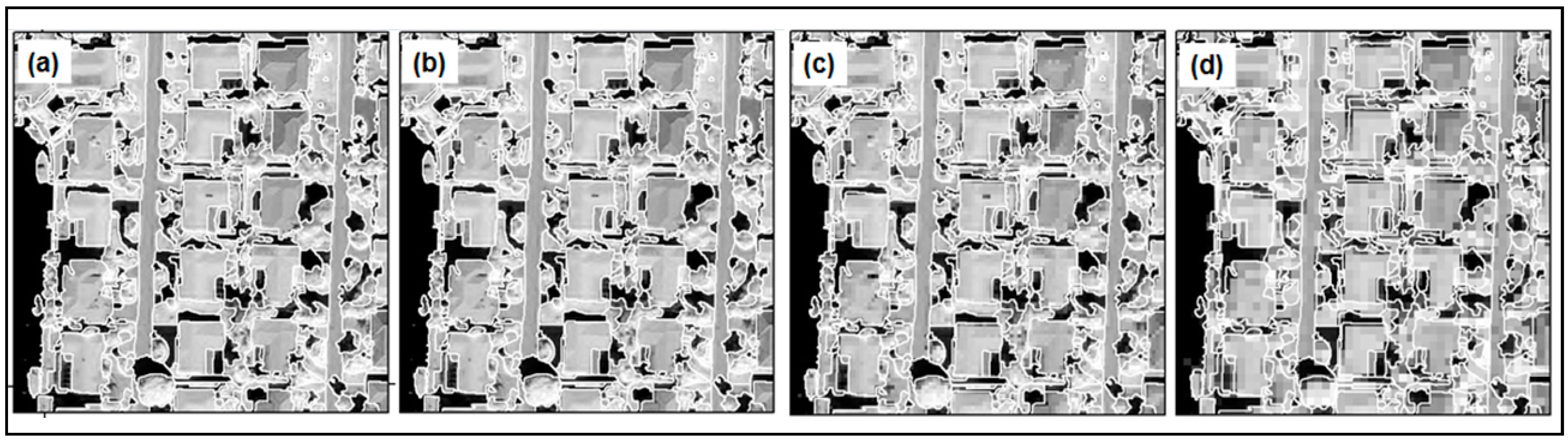
Figure 6. RapidEye image of a mixed agricultural/forested area (a) and the baseline object-based classification of this image (b). Classification results using SWSF (c) and USF (d) to extract spectral values (NDVI) from a simulated 30 m resolution image. Green represents “vegetation” and gray represents “non-vegetation” land cover. Colored rectangles highlight some areas with significant differences between the SWSF and USF classification results.

Figure 6. RapidEye image of a mixed agricultural/forested area (a) and the baseline object-based classification of this image (b). Classification results using SWSF (c) and USF (d) to extract spectral values (NDVI) from a simulated 30 m resolution image. Green represents “vegetation” and gray represents “non-vegetation” land cover. Colored rectangles highlight some areas with significant differences between the SWSF and USF classification results.

3.3. General Discussion

Based on the results of this study, SWSF can be useful for deriving descriptors of image segments from LSR images, such as high spectral or temporal resolution information, and has the potential to increase the accuracy of subsequent analysis performed on the segments (e.g., classification, extraction of biophysical parameters based on the spectral values of segments, etc.) when the ratio of the LSR to HSR image resolution is greater than 2:1. Unlike pixel-level fusion methods, which typically work best for fusing images with similar spectral ranges and/or similar acquisition dates [21], SWSF can be easily applied for fusing any type of imagery (e.g., fusing visible and synthetic aperture radar imagery, visible and thermal imagery, etc.) because it is insensitive to the correlation between the HSR and LSR images. However, since in many cases pixel-level fusion can be useful for image analysis tasks such as image classification [22,23,24,25], it should be emphasized that pixel-level fusion could also be performed in combination with SWSF. For example, instead of simply resampling the LSR image to match the HSR image (as was done in this study), a pixel-level image fusion method could first be applied to the LSR image to enhance its spatial quality, and then mean segment values could be extracted from the spatially-enhanced LSR image (instead of the resampled LSR image) using SWSF. Future work could investigate whether this combination of pixel- and segment-level fusion leads to more accurate image analysis than either fusion method alone, and whether it is worth the extra processing time/effort.

It should also be noted that the applications of SWSF are not limited to the extraction of spectral information for image segments (polygons) generated by an automated segmentation algorithm, and in theory can be used for any type of image-to-polygon fusion. For example, it could be used to fuse an image with OpenStreetMap building footprint polygons to extract the reflectance properties of individual rooftops (e.g., for estimating the energy savings potential of the building [26]), or to fuse an image with manually-digitized polygons of agricultural fields to extract crop-related parameters for each field. Investigation of SWSF (and other image-to-polygon fusion methods) for these types of fusion tasks could also be an interesting future research topic.

4. Conclusions

A spatially-weighted segment-level fusion (SWSF) method was proposed for fusing lower spatial resolution (LSR) images with higher spatial resolution (HSR) images at the image segment level. It involves segmenting a higher spatial resolution (HSR) image and then extracting additional descriptors (mean segment values) from LSR images using a spatially-weighted calculation method. SWSF extracted more accurate spectral information of land cover features than the traditional unweighted segment-level fusion (USF) approach when the ratio of the LSR image resolution to the higher spatial resolution (HSR) image was 3:1 (0.9 m LSR image:0.3 m HSR image) or higher. SWSF was also found to increase image classification accuracy, particularly for segments that were small or narrow relative to the spatial resolution of the LSR image (i.e., segments containing a high proportion of mixed pixels along their boundary). From these results and based on the geometry of LSR and HSR pixels, SWSF is recommended for segment level fusion when the spatial resolution of LSR image relative to that of the HSR image is higher than 2:1. Future research is necessary to assess the impact of SWSF on other types of image analysis (e.g., regression tasks).