Abstract
Top-k spatial preference queries rank objects based on the score of feature objects in their spatial neighborhood. Top-k preference queries are crucial for a wide range of location based services such as hotel browsing and apartment searching. In recent years, a lot of research has been conducted on processing of top-k spatial preference queries in Euclidean space. While few algorithms study top-k preference queries in road networks, they all focus on undirected road networks. In this paper, we investigate the problem of processing the top-k spatial preference queries in directed road networks where each road segment has a particular orientation. Computation of data object scores requires examining the scores of each feature object in its spatial neighborhood. This may cause the computational delay, thus resulting in a high query processing time. In this paper, we address this problem by proposing a pruning and grouping of feature objects to reduce the number of feature objects. Furthermore, we present an efficient algorithm called TOPS that can process top-k spatial preference queries in directed road networks. Experimental results indicate that our algorithm significantly reduces the query processing time compared to period solution for a wide range of problem settings.
1. Introduction
Due to the exponential growth of hand held devices, the widespread availability of maps and inexpensive network bandwidths have popularized location based services. According to Skyhook, the number of location-based applications being developed each month is increasing exponentially. Thus, spatial queries such as nearest neighbor, range queries and reverse nearest neighbor [1,2,3,4,5] have received a significant amount of attention from the research community. However, most of the existing applications are limited to traditional spatial queries, which return objects based on their distances from the query point.
In this paper, we study the top-k spatial preference query, which returns a ranked list of best spatial objects based on the neighborhood facilities. Given a set of data objects , a top-k spatial preference query retrieves a set of objects in D based on the quality of the facilities (the quality is calculated by aggregating the distance score and non-spatial score) in its neighborhood. Many real-life scenarios exist to illustrate the useful-ness of preference queries. Thus, if we consider a scenario in which a real estate agency office maintains a database of available apartments, a customer may want to rank the apartments based on neighboring facilities (e.g., market, hospitals, and school).
In another example, a tourist may be looking for hotels, where he may be interested in hotels located near some good quality restaurants, cafes or tourist spots. Figure 1 illustrates the data objects (i.e., hotels) as triangles, and two distinct feature datasets: solid rectangles denote cafes while hollow rectangles denote restaurants. The number on each edge denotes the cost of traveling on that edge, where the cost of an edge can be considered as the amount of time required to travel along it e.g., . The numbers in parentheses over the feature objects denote the score of that particular feature object e.g., the score of feature object is 0.5. Now, let us consider a tourist looking for a hotel near to cafes and restaurants. The tourist can restrict the range of the query so we assume that range is 3 (i.e., ) in this example. The score of the hotels can be determined according to the following criteria (1) the maximum quality for each feature in the neighborhood region; and (2) the aggregate of these qualities. For instance, if the hotels are ranked based on the scores of cafes only, the top hotel would be because the score of and are 0.7, 0 and 0.5, respectively. It should be noted that the score of is 0 although is within its range, because it is a directed road network and no path connects to . On the contrary, if the hotels are ranked based only on the scores of restaurants, the top hotel would be because the score of and are 0, 0.8 and 0.5, respectively. Finally, if the hotels are ranked based on the summed scores of restaurants and cafes, then the top hotel would be because the score of and are 0.7, 0.8 and 1, respectively.
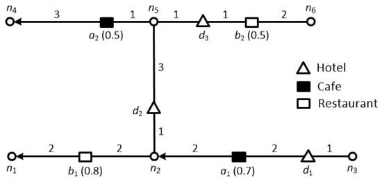
Figure 1.
Example of top-k spatial preference queries in a directed road network.
Two basic factors are considered when ranking objects: (1) the spatial ranking, which is the distance and (2) the non-spatial ranking, which ranks the objects based on the quality of the feature objects. Our top-k spatial preference query algorithm efficiently integrates these two factors to retrieve a list of data objects with the highest score.
Unlike traditional top-k queries [6,7], top-k spatial preference queries require that the score of a data object is defined by the feature objects that satisfies a spatial neighborhood condition such as the range, nearest neighbor, or influence [8,9,10,11]. Therefore, a pair comprising a data object and a feature objects needs to be examined in order to determine the score of the corresponding data object. In addition, processing top-k spatial preference queries in road networks is more complex than in Euclidean space, because the former requires the exploration of the spatial neighborhood along the given road network.
Top- spatial preference queries are intuitive and they have several useful applications such as hotel browsing. Unfortunately, most of the existing algorithms are focused on the Euclidean space and little attention has been given to road networks. Indeed, although few algorithms exist for the preference queries in road networks, they all consider undirected road networks. Motivated by aforementioned reasons, we propose a new approach to process top- spatial preference queries in directed road networks, where each road segment has a particular orientation (i.e., either directed or undirected). In our method, the feature objects in the road network are grouped together in order to reduce the number of pairs that need to be examined to find the top- data objects. We propose a method for grouping feature objects based on pivot nodes; as described in detail in Section 4.2.1. All of the pairs of data objects and feature groups are mapped onto a distance-score space, and a subset of pairs is identified that is sufficient to answer spatial preference queries. In order to map the pairs, we describe a mathematical formula for computing the minimum and maximum distances in directed road networks between data objects and feature groups. Finally, we present our Top-k Spatial Preference Query Algorithm (TOPS), which can efficiently compute the top-k data objects using these pairs.
This study is an extended version of our previous investigation of top-k spatial preference queries in directed road networks [12]. However, we present four new extensions that we did not consider in our preliminary study [12]. The first extension is an enhanced grouping technique which can efficiently obtain multiple feature groups associated with a single pivot node (Section 4.2.1). The second extension studies adaptations of the proposed algorithms to deal with neighborhood conditions other than range score, e.g., nearest neighbor score and influence score (Section 5). In the third extension, we present an efficient incremental maintenance method for materialized skyline sets (Section 5). In the fourth extension, we conduct an extensive experimental study in which we increase the number of parameters to evaluate the performance of TOPS; as well as implementing two versions of TOPS: and where we compared their performance with the Period approach (Section 6). In addition to these major extensions, we also present a Lemma to prove that the materialized skyline set is sufficient for determining the partial score of a data object . Furthermore, we also discuss the limitations of undirected road networks based algorithms in a directed road networks (Section 4.4).
The contributions of this paper are summarized as follows:
- We propose an efficient algorithm called TOPS for processing top-k preference queries in directed road networks. To the best of our knowledge, this is the first study to address this problem.
- We present a method for grouping feature objects based on a pivot node. We show the mapping of data objects and feature groups in a distance-score space to generate a skyline set.
- We state lemmas for computing the minimum and maximum distances between the data object and the feature group.
- In addition, we propose a cost-efficient method for the incremental maintenance of materialized skyline sets.
- Based on experimental evaluations, we study the effects of applying our proposed algorithm with various parameters using real-life road dataset.
The remainder of this paper is organized as follows. We discuss related research in Section 2. In Section 3, we define the primary terms and notation used in this study, as well as formulating the problem. In Section 4, we explain the pruning and grouping of feature objects, as well as mapping of pairs of data objects and feature groups to a distance-score space. Section 5 presents our proposed algorithm for processing top-k spatial preference queries in directed road networks. Our extensive experimental evaluations are presented in Section 6. Finally, we give our conclusion in Section 7.
2. Related Work
In this section, we review the previous algorithms proposed for ranking spatial data objects. Object ranking is a popular retrieval task in various applications. As found in most relational database applications, we often want to rank the tuples using an aggregate score of attribute values. For example, a rental car agency maintains a database that contains information about cars available for rent. A potential customer wishes to view the top 10 options among the latest models with the lowest prices. In this case, the score of each car is expressed by the sum of two qualities: model and price. In spatial databases, the rankings are often associated with nearest neighbor queries. Thus, given a query point q, we are mainly interested in finding the set of nearest objects to it that meet a specific condition. Many algorithms [1,13,14,15] have been proposed to retrieve the nearest neighbor objects both in Euclidean space and road networks.
In the following subsections, we survey the skyline queries in Section 2.1, as well as briefly review the feature-based spatial queries in Section 2.2, and top-k spatial preference queries in Section 2.3.
2.1. Skyline Queries
In recent years, skyline query processing [16,17,18,19,20,21] has attracted much of attention due to its suitability for decision-making applications such as top-k spatial preference queries. Lin et al. [16] studied the general spatial skyline (GSSKY) problem, which generates a minimal candidate set comprising the optimal solutions for any monotonic distance-based spatial preference query. They proposed an efficient progressive algorithm called P-GSSKY, which considerably reduces the number of non-promising objects during computation. Lee et al. [17] proposed two index-based approaches, called the augmented R-tree and dominance diagram for various skyline queries in Euclidean space, e.g., location-dependent skyline queries and reverse location-dependent skyline queries. Liu et al. [18] presented an algorithm for traditional top-k queries in road networks, which considers multiple attributes of data objects, including the data object’s location. For example, when a user wants to find a hotel, they often consider several factors such as the distance to the hotel, the hotel rating, and the service quality. However, their method does not consider the relationship between a data object and a feature object; therefore, it cannot be applied to top-k spatial preference queries in road networks. Deng et al. [19] was the first to consider the problem of multi-source skyline queries in road networks. Recently, Cheema et al. [22] addressed skyline queries for moving queries, where they proposed a safe zone based algorithm for continuously monitoring a skyline query.
2.2. Feature-Based Spatial Queries
Xia et al. [23] proposed a novel algorithm for retrieving the top-t most influential spatial sites (e.g., residential apartments) based on their influence on the feature points (e.g., market). The influence of each site p is determined by the sum of the scores of all the feature objects with p as their closest site. Yang et al. [24,25] studied the problem of finding optimal location queries, however, unlike [23] the optimal location query retrieves any point in the data space and it is not necessarily an object in the dataset; although the score computation method is similar [23]. These algorithms [23,24,25] are specific to the particular query types mentioned above and they cannot be applied to the top-k spatial preference queries. In addition, they only deal with the single feature dataset whereas preference query considers a multiple feature dataset.
2.3. Top-k Spatial Preference Queries
Several algorithms have been proposed for top-k spatial preference queries in Euclidean space. Yiu el al. [8,9] first considered computing the score of data object p based on the set of multiple feature objects in its spatial neighborhood rather than a single feature object set as studied previously [21,22,23]. We know that the score of a data object can be defined by three different spatial scores, i.e., the range, nearest neighbor, and nearest score; thus, Yiu et al. [8,9] designed several algorithms according to three categories (Probing Algorithms, Branch and Bound Algorithms, and Feature Join Algorithms) for evaluating the top-k spatial preference queries for these scores. In contrast to Yiu et al. [8,9], Rocha-Junior et al. [10] proposed a materialization technique which yields significant computational and I/O cost savings during query processing. They introduced a mapping of pairs of the data object and the feature object to a distance-score space. The minimal subset of the pairs is materialized and it is sufficient to answer any spatial preference query in an efficient manner. However, these Euclidean space based algorithms [8,9,10] are not suitable for evaluating top-k spatial preference queries in road networks because the distance between objects is determined by the shortest path connecting them in road networks.
Cho et al. [11] proposed a novel algorithm called ALPS for processing top-k preference queries in road networks, where they extended the materialization technique [10] based on the distance-score space for road networks. To minimize the number of data objects, their methodology groups a set of data objects in a road segment and then converts grouped data objects into a data segment. ALPS [11] can efficiently process the top-k spatial preference queries in road networks, but it only works for undirected road networks.
This study distinguishes itself from existing studies in several aspects. Firstly, we study top-k spatial preference queries in a directed road network where each road segment has a particular orientation whereas the previous studies they either focus on Euclidean space [8,9,10] or an undirected road network [11]. Secondly, our approach is based on the grouping of feature objects, which reduces the computation cost. Lastly, we devise a mathematical formula to quickly calculate the minimum and maximum distances between the data object and the feature group in the road network. In recent years, different variations of preference queries have been studied in spatial road networks. Mouratidis et al. [26] studies preference queries in multi-cost transportation network where each road segment is associated with multiple cost values. Lin et al. [27] studies k multi-preference queries to retrieve top-k groups of facilities that minimizes the traveling distance in the road network. These studies have different problem scenarios from those in our study and their solutions are not appropriate in our problem domain. Furthermore, we present detailed limitations of undirected based algorithms in directed road networks in Section 4.4.
3. Preliminaries
Section 3.1 defines the terms and notations used in this paper. Section 3.2 formulates the problem using an example to illustrate the results obtained from top-k spatial preference queries.
3.1. Definition of Terms and Notations
Road Network:
A road network is represented by a weighted directed graph (G = N, E, W) where N, E, and W denote the node set, edge set, and edge distance matrix, respectively. Each edge is also assigned an orientation, which is either undirected or directed. An undirected edge is represented by , where and are adjacent nodes, whereas a directed edge is represented as or . Naturally, the arrows above the edges denote their associated directions.
Segment s(pi, pj) is the part of an edge between two points p1 and p2 on the edge. An edge comprises one or more segments. An edge is also considered to be a segment where the nodes are the end points of the edge. To simplify the presentation, Table 1 lists the notations used in this study.

Table 1.
Summary of notations used in this study.
3.2. Problem Formulation
Given a set of data objects and a set of m feature dataset the top-k spatial preference query returns the k data objects with the highest scores. The score of a data object is defined by the scores of the feature objects in the spatial neighborhood of the data object. Each feature object f has a non-spatial score, denoted as s( f ), which indicates the quality (goodness) of f and it is graded in the range [0,1].
The score of a data object d is determined by aggregating the partial scores with respect to a neighborhood condition θ and the ith feature dataset Fi. The aggregation function ‘agg’ can be any monotone function (sum, max, min), but in this study we use the sum to simplify the discussion. We consider the range (rng), nearest neighbor (nn), and influence (inf) constraints as the neighborhood condition θ. In particular, the score is defined as, , where and .
The partial score is determined by the feature objects that belongs to the ith feature dataset Fi only and that satisfy the neighborhood condition θ. In other words is defined by the highest score s(f) for a single feature object that satisfies the spatial constraint θ. Similar to previous studies [9,10,11], the partial scores for different neighborhood conditions θ are defined as follows:
- Range(rng) score of d:
- Nearest neighbor (nn) score of d:
- Influence(inf) score of d:
Next, we evaluate the scores of data objects d1, d2 and d3 in Figure 1. We consider the range constraint value r = 3. Table 2 summarizes the scores obtained of d1, d2 and d3 using the aforementioned definitions of the neighborhood conditions {rng, nn, inf}.

Table 2.
Computation of the scores of data objects d1, d2, and d3.
The score of data object d is the sum of the partial score of each feature set. The range score of d1 is calculated as . The ith partial range score of a data object d is the maximum non-spatial score of the feature objects which are within the range r. Therefore, the first partial score , because and . However, because there is no restaurant located within the defined range r. Similarly, the range scores of d2 and d3 are and , respectively.
The nearest neighbor score of d1 is calculated as . The ith partial nearest neighbor score of a data object d is the score of the nearest feature object to d. Therefore, the first partial score , because a1 is the closest feature object of d1 and , whereas because b1 is the closest feature object of d1 and . Similarly, the nearest neighbor score of d2 and d3 are and , respectively.
The influence score of d1 is calculated as . The ith partial influence score of a data object d is calculated using the score of the feature object and its distance to the data object. Specifically, the influence score is inversely proportional to the distance between d and f. Therefore, the influence score decreases rapidly as the distance between the feature object f and data object d increases. The first partial score , because , , , and , whereas , because , , , and . Similarly, the influence score of d2 and d3 are and , respectively.
3.3. Finding Pivot Nodes
We now discuss the method used for computing the pivot nodes. In our approach, we group the feature objects based on the pivot nodes. Each feature object is associated with one pivot node, and thus feature objects sharing the same pivot node can be grouped together. It is obvious that the performance of the proposed scheme will improve if the number of feature groups is small. Therefore, the main objective is to retrieve the minimum number of pivot nodes. Computing the minimum number of pivot nodes is a minimum vertex cover problem. The minimum vertex cover comprises a set of nodes that can connect all the edges of the graph with the minimum number of nodes.
Definition 1:
A vertex cover of a graph is a subset such that if then either or or both. In other words, a vertex cover is a subset of nodes that contains at least one node on each edge.
The minimum vertex cover is an NP-complete problem and it is also closely related to many other hard graph problems. Therefore, numerous studies have been conducted to design optimization and approximation techniques based on Branch and Bound Algorithm, Greedy Algorithm and Genetic Algorithm. We employ the technique proposed by Hartmann [28] based on the Branch and bound algorithm because it is a complete algorithm, thereby ensuring that we find the best solution or the optimal solution of various optimization problems, including the minimum vertex cover. However, the only tradeoff when using Branch and Bound algorithm is that the running time increases with large graphs.
The Branch and Bound algorithm recursively explores the complete graph by determining the presence or absence of one node in the cover during each step of the recursive process, and then recursively solving the problem for the remaining nodes. The complete search space can be considered as a tree where each level determines the presence or absence of one node, and there are two possible branches to follow for each node; one corresponds to selecting the node for the cover whereas the other corresponds to ignoring the node. Virtually a node that is covered and all of its adjacent edges are removed from the graph. The algorithm does not need to descend further into the tree when a cover has been found, i.e., when all of the edges are covered. Next, the backtracking process starts and search continues to higher levels of the tree to identify a cover with a possibly smaller vertex cover. During backtracking all of the covered nodes are reinserted in the graph. Subsets of the nodes are determined that yield legitimate vertex covers and the smallest in size is the minimum vertex cover.
Let us consider an example in Figure 2, where we found that the set of nodes constructs a minimum vertex cover, that connects all of the edges in a given road network.
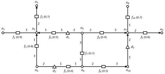
Figure 2.
Pruning and grouping example.
4. Pruning and Grouping
Top-k spatial preference queries return a ranked set of spatial data objects. Unlike traditional top-k queries the rank of each data object is determined by the quality of the feature objects in its spatial neighborhood. Thus, computing the partial score of a data object d based on the feature set Fi requires the examination of every pair of objects (d, f). Therefore, for a large number of objects, the search space that needs to be explored to determine the partial score is also significantly high, thereby further increasing the challenges of efficiently processing top-k spatial queries in directed road networks.
In Section 4.1, we discuss the dominance relation and we then explain the pruning lemma. Section 4.2 presents the grouping algorithm and the computation of the feature group score , as well as discussing the computation of the minimum and maximum distances between data objects and feature groups. Section 4.3 describes the mapping of pairs of data objects and feature groups to the distance-score space. Finally, we discuss the limitations of undirected based algorithms in directed road networks in Section 4.4.
4.1. Pruning
In this section, we present a method for finding the dominant feature objects that contribute only to the score of a data object. The feature objects that do not contribute to the score of a data object will be pruned automatically. This dramatically reduces the search space, thereby significantly decreasing the computational cost. In order to make the pruning step more efficient, we use the pre-computed distances stored in a minimum distance table MDT. The MDT stores the pre-computed distances between the pair of nodes ni and nj in a directed road network. Each tuple in a MDT is of the form , where is used as a search key for retrieving the value of . It should be noted that the network distance between two nodes, ni and nj, is not symmetrical in a directed road network (i.e., ). Therefore, we need to insert a separate entry to retrieve the distance from nj to ni. Figure 2 shows an example of a directed road network, which we employ throughout this section.
Before presenting the pruning lemma, let us define some useful terminologies:
Static Dimension:
The static dimensions i (i.e., ) are fixed criteria that are not changed by the motion of the query, such as the rank of any restaurant or price.
Static Equality:
An object o is statically equal to object if, for every static dimension i, . We denote the static equality as .
Static Dominance:
An object o is statically dominated by another object if is better than o in every static dimension. We use to denote that object statically dominates object o. We use to denote that either statically dominates o or is statically equivalent to o. In Figure 2, because the non-spatial score of f1 is better than that of f2 i.e., .
Complete Dominance:
To explain the pruning lemma we need to define complete dominance. An object o is completely dominated by another object with respect to data object d, if as well as . In other words, completely dominates o if is equally good in terms of its static dimensions and it is also closer to the data object d. In Figure 2, the feature object f1 completely dominates f2 with respect to because and . On the other hand, f4 is not completely dominated by f1, although but
Dominant Pair (DP):
Given two pairs and , is said to dominate , if and . The set of pairs that are not dominated by any other pair in are referred as dominant set .
Lemma 1:
A feature object is a dominant object if and only if for any other feature object f for which ,
Proof:
The proof is straight forward and thus it is omitted. Intuitively, a Lemma 1 state that is a dominant object if is closer to d than every other object f and it is at least as good as f in terms of its static dimensions (i.e., ).
In Figure 2, f2 is not a dominant object of d1 because a feature object f1 exists such that and . Hence, f2 is completely dominated by f1, and thus it is pruned, whereas, f4 is a dominant object because it is closer to d1. Here, note that f3 cannot be a dominant object for data object d1 because we are considering a directed road network and no path exists to f3 from d1.
Figure 3 depicts the mapping of to the distance-score space M. We formally define the distance-score space in Section 4.3. The black square shows the mapping of pairs where and . Now, by applying the dominance relationship onto the mapping in Figure 3a, we find that pair is completely dominated by . Therefore, . Figure 3b shows that and are dominated pairs. Similarly, Figure 3c shows the mapping of , and it is clear that both pairs and are not dominated by any other pair.
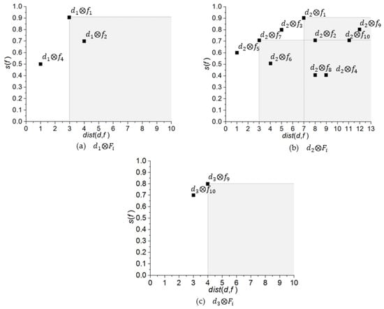
Figure 3.
Mapping of to the distance-score space. (a) ; (b) ; (c) .
4.2. Grouping
In this section, we describe our approach for grouping the feature objects. The pruning phase reduces the number of feature objects, but this can be reduced further by merging them into a group. In addition, the grouping technique reduces the size of skyline set and the entries in R-tree [29], thereby enhancing the efficiency of algorithm by minimizing the memory consumption required. As mentioned earlier, the score for data object d is computed from the score of the feature objects which requires that we examine every pair of objects (d, f). The performance of the algorithm will decline dramatically if the number of feature objects is excessively high. Therefore, the main purpose of grouping is to further reduce the number of feature objects by grouping them together, which consequently reduces the number of pairs. Thus, instead of evaluating the individual pairs , our algorithm evaluates evaluates , where g denotes a feature group and a set of feature groups are represented as Gi. Grouping the feature objects has two main advantages as follows.
- It is easy to compute the highest score of a data object.
- The computational cost and memory consumption are decreased by reducing the number of pairs.
4.2.1. Grouping Method
We now discuss the method for grouping feature objects based on pivot nodes. We have described the technique for finding the minimum pivot nodes in Section 3.3. For grouping, each feature object is associated with one of a pivot node. In pruning phase, we find the dominant feature objects for each data object. The dominant feature objects of each data object are grouped together if they are associated with the same pivot node. In our previous study [12], we grouped all the feature objects connected to one pivot node, thereby generating one feature group per pivot node. However, in some cases, more than one feature group may be associated with a single pivot node if dominant feature objects of multiple data objects share the same pivot node.
Let us consider the same example shown in Figure 2, where node is the pivot node and the feature objects f1, f2, f3, and f4 are connected to it. As mentioned in Section 4.1, for data object d1 the dominant objects are f1 and f4 whereas feature object f2 and f3 are pruned. However, for data object d2; f1 and f3 is dominant whereas f2 and f4 are pruned. Therefore, two groups are formed and which are associated with pivot node . Table 3 summarizes the grouping of feature objects.

Table 3.
Summary of the grouping of feature objects.
4.2.2. Computation of the Group Score
Due to the separate score of each feature object, the computation of partial score becomes costly for a large number of feature objects. We devised a new method for calculating the partial scores based on the group score denoted as . The group score is the highest score for any feature object that belongs to a group such that it qualifies the neighborhood conditions. Table 3 shows that , and . Therefore, which is the highest score of the feature object belongs to . The score of other groups can be computed in a similar fashion.
The partial score by using can be defined as follows:
- Range(rng) score of d:
- Nearest neighbor (nn) score of d:
- Influence(inf) score of d:
We modify the formulae presented in Section 3.2 to compute the partial score by using the group score instead of the feature score . The only difference is is used instead of for range and influence score whereas is used instead of for nearest neighbor score.
4.2.3. Computation of the Distance between a Data Object and Feature Group
In this section, we present Lemmas for the computation of the minimum and maximum distances between a data object and feature group. The subset of pairs retrieved in the grouping step is indexed in an R-tree [17], where it is necessary to compute the minimum and maximum distances between a data object and feature group. Lemma 2 presents the computation of , while Lemmas 3 and 4 describe the computation of for and , respectively.
Lemma 2:
Given a data object and a feature group g, is as follows:
Proof:
This lemma is self-evident, so the proof is omitted. Here, denotes the boundary point of feature group. For , ,
We consider a directed road network and thus to determine , it is necessary to evaluate and where, and refer to directed and undirected segments, respectively. To compute , we consider the two cases separately: (1) and (2) . For we use the method proposed by Cho et al. in [11].
Lemma 3:
If , then there are following two cases:
(Case 3a):
If a path from to exists,
Proof:
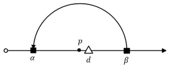
Let us suppose that and β are the boundary points on the road segment that belongs to a feature group and data object d is located between As shown in Figure 4, there exists a point p such that . According to Figure 4, it is obvious that . From the equation above, we can observe that the distance value will increase with the value of , so to obtain the maximum distance value, the point p must be very close to d, and thus we can say that . Therefore, we can rewrite the equation above as which is equal to .

Figure 4.
Determination of when .
(Case 3b):
If no path exists from to ,
Proof:
This lemma is self-evident, so the proof is omitted.
Lemma 4:
If , then is as follows:
Proof:
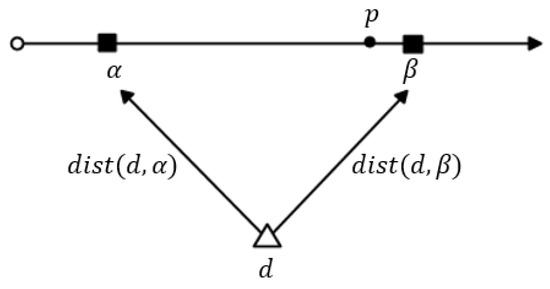
According to the definition . As shown in Figure 5, it is obvious that we obtain the maximum distance from d to p when point p is located very close to , and thus we can say that . Two paths exist from d to : and , and thus or Therefore, we can say that .

Figure 5.
Determination of when .

Table 4.
Summary of in Figure 2.
4.3. Mapping to Distance-Score Space
In this section, we formally define the search space of the top-k spatial preference queries by defining a mapping of the data objects d and any feature group g to a distance-score space. Let denote a pair comprising data object and a feature group , then is represented as . Each pair is mapped to either a point or a line segment in the distance-score space M, defined by the axes and , where corresponds to the distance between data object d and feature group g and corresponds to score of .
Definition 2:
(Mapping of to M): The mapping of pairs comprising a data object and a feature group to the 2-dimensional space M (called distance-score space) is .
In the following, we define the dominance relation which is the subset of pairs of M that comprise the skyline set of M, denoted as . The skyline set S is the set of pairs which are not dominated by any other pair .
Definition 3:
(Dominance ): Given two pairs is said to dominate another pair , denoted as , if and or if and .
Let be the set of all pairs that are not dominated by any other pair in . Figure 6 shows the mapping of in Table 4 to the distance-score space M. Figure 6a shows the mapping of , Figure 6b shows the mapping of and Figure 6c shows the mapping of . The skyline sets of , and are , and , respectively. The pairs related to different data objects (e.g., and ) are definitely incomparable. Finally, the skyline set for is the union of the skyline sets of all the data objects . Thus, Figure 6d shows the skyline set, .
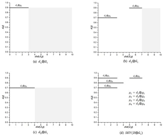
Figure 6.
Mapping to distance-score space. (a) ; (b) ; (c) ; (d) .
Observe that in Figure 6a, is mapped at 0.9 because . It should be noted that can be changed according to the neighborhood conditions. As explained earlier, because and . Now, if we consider range condition , the , because , which does not satisfy the neighborhood condition. In this scenario, the is changed to 0.5 which is the score of . Thus, is mapped at 0.5.
Figure 7a shows the mapping of to M. Figure 7b, on the other hand, shows an R-tree that indexes the four pairs in , assuming that node capacity of R-tree is set to 3. Therefore, index node R2 encloses and , whereas index node R3, encloses and . Finally, we present Lemma 5, which proves that is sufficient for determining the partial score of each data object Before presenting Lemma 5, recall that each feature object is a dominant feature object and not dominated by any other feature object .
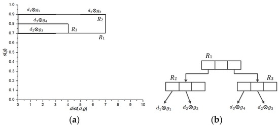
Figure 7.
Mapping to distance-score space. (a) ; (b) R-tree representation for .
Lemma 5:
For any spatial preference query, is sufficient for determining the partial score of a data object .
Proof:
Let us assume that is not sufficient for obtaining the partial score of a data object . This means that there is a feature group that contributes to . Now if or , then , and if , then . However, a pair such that there is another pair and which is equivalent to either and or if and . Hence, the partial score of d is if or , and if . This contradicts our assumption that contributes to . Therefore, is sufficient for obtaining the component score of a data object .
4.4. Limitations of Undirected Algorithms in Directed Road Networks
In contrast to undirected road networks, the network distance between two nodes is not symmetrical in directed road networks, i.e., . Figure 8a shows an undirected road network, where there are two data objects d1 and d2, and two feature objects f1 and f2. To simplify the presentation, we consider a single feature dataset .

Figure 8.
Examples (a) undirected road network; (b) directed road network.
Let us now evaluate the scores of the data objects. Suppose that the neighborhood condition is the range and value of the range constraint r = 3. The range score of d1 is 0.8 because and . Similarly, the range score of d2 is 0.6 because and . Therefore, d1 is the top-1 result with .
Now, assume the directed road network as shown in Figure 8b. In this case, the range score of d1 is 0 because no feature object exists within distance r. However, the range score of d2 remains the same because f1 still exists within distance r. Therefore, in the directed road network, d2 is the top-1 result with . This example clearly demonstrates that an algorithm based on an undirected road network cannot be applied to directed road networks.
The research study closest to our present work was presented by Cho et al. [11]. They proposed an algorithm called ALPS for processing preference queries in undirected road networks, where the data objects in a road sequence are grouped to form a data segment in their approach. The motivation behind grouping data objects is that data objects in a sequence are close to each other, so it is more efficient to process them together rather than handling each data object separately. However, ALPS fall short in answering preference queries in directed road networks.
Now, we present why ALPS cannot process preference queries in directed road networks. Consider a directed road in Figure 9 where there are four data objects d1, d2, d3 and d4 and two feature objects f1 and f2 which are denoted as triangles and rectangles, respectively. The data objects d1 and d2 lies in a same sequence are grouped and converted to data segment and data objects d3 and d4 are converted to . Observe that, grouping of is not valid because there is no path that exists to connect d3 to d4, as shown in Figure 9.
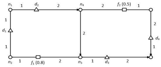
Figure 9.
Example of ALPS in directed road network.
Another issue is indexing of data segments and feature object pairs in R-tree for directed road networks. Let denote a pair that consists of a data segment dseg and feature object f. To index a pair in R-tree it is necessary to compute minimum and maximum distances between data segment dseg and a feature object f. In Figure 9, as per ALPS computation and . Conversely, the actual . ALPS computes the minimum and maximum distances between the data segment and the feature object based on the assumption that , but this assumption is not applicable in a directed road network where . Thus, ALPS generates an erroneous R-tree which leads to incorrect results. The above example demonstrates that ALPS do not work for directed road networks. For ALPS, to answer preference queries in a directed road network, the method for grouping and computing and should be modified to consider the particular orientation of each road segment.
Comparing ALPS and TOPS conceptually, ALPS adopts the grouping of data objects into data segments whereas TOPS groups the feature objects. ALPS first groups the data objects to data segments and then prunes the dominated pairs which may allow the redundant pairs in the R-tree. However, TOPS first prune the pairs to avoid any redundant pair and then group them based on pivot nodes. Therefore, query processing time can be high in ALPS. Similarly, due to a higher number of redundant pairs, ALPS might utilize more disk size for indexing of skyline sets. However, the index construction time of ALPS can be better than TOPS because a lower number of skyline sets needs to be generated due to grouping of data objects.
5. Top-k Spatial Preference Query Algorithm
In this section, we present the Top-k Spatial Preference Query Algorithm (TOPS), for top-k spatial preference queries. TOPS is appropriate for all three neighborhood conditions (range, nearest neighbor and influence), but we discuss the range constraint to simplify the explanation. We then present the necessary modifications for supporting nearest neighbor and influence scores. Our algorithm processes the top-k preference query by sequential accessing the data objects in descending order of their partial score. In order to achieve this, TOPS retrieves qualifying data objects, one by one during query processing in descending order based on their partial scores, which can rapidly produce a set of k top data objects with the highest scores.
Algorithm 1 computes the top-k data objects with the highest score by aggregating the partial scores of data objects retrieved from each max heap Hi. For each skyline set, , we employ a max heap Hi to traverse the data objects in descending order of their component score. Whenever the method is called, the data object dhigh with the highest component score is popped from the max heap Hi. Let Dk be the current top-k set and Ri is the recent component score seen in Hi. In addition, TOPS maintains a list of candidate data objects Dc, which may become top-k data objects. Ri is set to (line 6) and the lower bound score is also updated using the aggregate function (line 7). If the number of data objects in Dk is less than k or is greater than the k-th highest score of data object in Dk, then dhigh is added to Dk. If dhigh is already in Dc then it will be removed from the Dc list. If the number of data objects in Dk = k + 1, the data object with the lowest is moved from Dk to Dc (line 8–12). Then, t is set to the lowest of the data objects in Dk (line 13). The upper bound score is computed for each data object .
| Algorithm 1: TOPS(Hi,k,r) | |||||
| Input: Hi: a max heap with entries in descending order of partial range score, k: number of requested data objects with highest score, r: range constraint | |||||
| Output: Top-k data objects with highest score | |||||
| 1: | /* set of candidate data objects */ | ||||
| 2: | /* current Top-k set */ | ||||
| 3: | /* Recent partial score seen in Hi | ||||
| 4: | while ∃Hi such that do | ||||
| 5: | |||||
| 6: | /* pop data object with highest score from Hi*/ | ||||
| 7: | |||||
| 8: | If number of data objects in or then | ||||
| 9: | |||||
| 10: | if then | ||||
| 11: | if number of data objects in then | ||||
| 12: | and | ||||
| 13: | |||||
| 14: | else | ||||
| 15: | /* If then add it in Dc*/ | ||||
| 16: | for each data object do | ||||
| 17: | |||||
| 18: | If then | ||||
| 19: | |||||
| 20: | If and number of data objects in then | ||||
| 21: | break while statement | ||||
| 22: | Return Dk | ||||
Finally, for each candidate object in Dc, the upper bound score is computed by . The maximum is then set to u (lines 16–19). If then no newly observed data object will end up in Dk. Therefore, the algorithm terminates and returns Dk if and the number of data objects in , or if all the heaps are exhausted (lines 20–22).
In order to illustrate our proposed algorithm, let us consider the example presented in Figure 7, where the R-tree is shown to index the skyline set that have been constructed using the example in Figure 2. We recall that hotels correspond to the data objects and cafes correspond to the feature objects . Let us consider that the client requested the following query of the top-k spatial preference query: “Find two hotels that are associated with a high-grade cafe which are located within a distance of 4”. We recall that in this query, and . After pruning and grouping the final generated skyline set is shown in Figure 7a, . The algorithm checks all the qualifying pairs based on the neighborhood condition Three pairs and are retrieved one at a time from R, and pushed onto a max heap H. Thus, . Finally, d1 and d3 are selected as the Top-2 query result because they have scores of 0.9 and 0.8, respectively.
Algorithm 2 returns the data objects one by one in descending order based on their partial score . Initially, the heap Hi contains the root node of an R-tree. Hi comprises records rc, which can be either the data object or the R-tree node. Each time the record rc with the highest partial score is popped from Hi. If rc indicates an R-tree node (line 3), then the algorithm verifies if the feature group satisfies the neighborhood condition . If entry s satisfies the neighborhood condition, it is added into (line 4, 5). If it does not satisfy neighborhood condition, which means a feature object exists such that . Therefore, each feature object needs to be examined to verify that (line 8). All the qualifying records are inserted to Heap Hi and the highest score of each feature object is assigned as a group score s(g) (lines 9, 10). Finally, when data object d is found, it is returned as with the highest partial score (lines 15, 17).
Algorithm 2 can be adapted with minor modifications to the nearest neighbor and influence scores. For the nearest neighbor score, the pairs are pruned such that f is not the nearest neighbor of d. Thus, during the construction of , the data objects are flagged to indicate whether or not f is the nearest neighbor of d (bit 1 if f is the nearest neighbor, and a 0 bit otherwise). For the influence score, the radius r is only used to compute the score and the score of feature object is reduced in proportion to the distance to a data object. Therefore, the verification conditions from Algorithm 2 (lines 4 and 8) are removed from the algorithm for the influence score. Thus, for each feature object , the component influence score is computed with respect to feature object and a corresponding entry is added to .
| Algorithm 2: NextHighestRangeScore(Hi,r) | ||
| Input: Hi: a max heap with entries in descending order of partial range score, r: range constraint | ||
| Output: The next data object in Hi with highest partial score | ||
| 1: | ||
| 2: | while do | |
| 3: | for each record c do | |
| 4: | if then | |
| 5: | Push record s to Hi | |
| 6: | else | |
| 7: | for each feature object do | |
| 8: | if then | |
| 9: | Push record s to Hi | |
| 10: | compute | |
| 11: | end if | |
| 12: | end for | |
| 13: | end if | |
| 14: | end for | |
| 15: | ||
| 16: | end while | |
| 17: | return rc | |
Incremental Maintenance
In this section, we discuss the incremental maintenance of the skyline set during the insertion, deletion and updating processes of the data and feature objects. We use the adaptation of the branch-and-bound skyline (BBS) the dynamic skyline algorithm for incremental maintenance of the skyline set. First, we update which is retrieved during the pruning phase and the Skyline set is then updated based on the updated set. Once the dominant set is updated, the update of group and is simple and straight forward. Insertions and deletions of data objects are fairly simple and cost-effective. When a new data object dnew is inserted into D, all of the dominant pairs are added to the set and the feature objects with the same pivot node form a feature group Next, the pairs are inserted in skyline set . If a data object ddeleted is deleted, then the pairs are deleted from the skyline set and all of the pairs are deleted from the set. Updates to the spatial location of a data object d are processed as a deletion followed by an insertion.
Next, we discuss the insertion, deletion and update processes of feature objects. The scores of feature objects are usually updated more frequently compared with the spatial location. Therefore, the most frequent maintenance operation is updating the score of a feature object. Updating the score of a feature object can potentially affect the score of a group which may affect the materialized skyline set . However, the updating cost is not very high due to the dominance relationship. Let us assume that the score of a feature object fupdated has been updated. As a consequence, the following two cases may occur: (1) the dominant set is still valid, (2) the dominant set is no longer valid. In the first case, if the set is valid, this means that the materialized skyline sets are also valid so there is no need for maintenance and the score of fupdated is simply updated. If fupdated has the highest score in the group, then the score of the group is also updated. In the second case, we check the dominance relationship. Only the score of the feature object is updated, so the maintenance algorithm simply performs a static dominance relation to update the set. First, we check whether , and the pairs are then removed from the set. Next, we check whether any feature object is dominated by fupdated. If , then the pairs are removed from the sets. Finally, the information regarding the groups (i.e., max/min distance and s(g)) is modified based on updated set and is generated.
Let us consider the addition of a new feature object fnew to the feature object set Fi. First, we need to execute the dominance check. If a pair is dominated by any other pair in set, this does not affect the dominant set, so it is simply discarded. However, if it is not dominated by any other pair then the maintenance algorithm will issue a query to retrieve all of the pairs that are dominated by . If no pair is retrieved then is simply added to the set, otherwise, the maintenance algorithm will remove all of the existing pairs from that are dominated by . Similarly, the information regarding groups is changed based on the updated set and is generated.
Next, we explain the maintenance of the skyline set after the deletion of feature objects. First, we need to check whether . If , then no further processing is required; otherwise, the maintenance algorithm is called. For incremental maintenance, we need to determine the set of pairs that are exclusively dominated by . If such pairs exist, then the dominant pairs are computed for these pairs and added to set; otherwise, is simply removed from the set. Finally, as mentioned earlier, the information regarding groups is modified based on the updated set and is generated.
Finally, we analyze the time complexities of adding, deleting, and updating a data object and a feature object. As mentioned earlier, incremental maintenance is performed on instead of ; therefore, we analyze the time complexity in terms of updating and maintaining . The time complexity of adding a data object is , where m is the number of feature datasets. Specifically, the dominant set of is generated for each feature dataset m which has a time complexity of . Then, the dominant set is updated which has a time complexity of . The time complexity of deleting a data object is . Thus, the time complexity of updating a data object is because updating a data object can be handled by a deletion of data object followed by an insertion.
The time complexity of adding a feature object is . This is because for each pair , the dominance check is performed to verify whether dominates or whether is dominated by . Next, we analyze the time complexity of deleting a feature object . Let be the set of pairs that are exclusively dominated by . For each data object , the exclusive dominance region for is determined, which has the time complexity of ). Then, the dominant set for the pairs that are exclusively dominated by is determined which has the time complexity of . Thus, the time complexity of deleting a feature object is . Lastly, the time complexity of updating a feature object is because the update (i.e., location or score update) of a feature object can be handled as a deletion followed by an insertion.
6. Performance Evaluation
In this section, we describe the performance evaluation of our proposed algorithm TOPS based on simulation experiments. In Section 6.1, we describe our experimental settings. Section 6.2 presents the experimental results for query processing time. Section 6.3 studies the performance evaluation of materialization and maintenance costs. Finally, in Section 6.4, we present the performance comparison of TOPS and .
6.1. Experimental Settings
All of our experiments are performed using a real road network [30] that comprises the main roads of North America, with 175,812 nodes and 179,178 edges. According to the American Hotel and Lodging Association [31], at the end of year 2014, there were 53,432 hotels in the United States, which corresponds to the data objects in this study. All of the algorithms were implemented in Java and run on a desktop PC with a Pentium 2.8 GHz processor and 4 GB memory. The datasets were indexed by R-trees with a page size of 4 KB. Our results comprised the average values obtained from 20 experiments. In all of the experiments, we measured the total query processing time with respect to various parameters, as shown in Table 5. In each experiment, we only varied one parameter whereas the others remained fixed at the bold default values.

Table 5.
Experimental parameter settings.
We implement and evaluate two versions of TOPS: and . groups the feature objects and then generates and stores the skyline set , whereas, does not group the feature objects, but instead it generates and stores the skyline set for each data and feature object pair . We compare both versions of TOPS with the Period approach, which computes the score for every data object by using the incremental network expansion (INE) and range network expansion (RNE) algorithms [32] to compute the nearest neighbor and range scores, respectively. The INE algorithm finds k nearest neighbors in road networks using Dijkstra’s algorithm [33]. The RNE algorithm is similar to the INE algorithm, except that it explores the network within a distance r from a query point. We slightly modified the RNE algorithm in order to compute the influence scores of data objects. The Period method does not use any materialization scheme.
6.2. Experimental Results for Query Processing Time
Figure 10 shows the query processing times for , and the Period method for the range condition. Figure 10a shows the query processing time as a function of the number k of requested data objects with the highest score. The query processing time of the period method incurs a constant query processing time regardless of the value of k because it explores all the feature objects within the query range r of the data object. However, the query processing time of and increases slightly with the value of k. Nevertheless, and outperform period algorithm. Figure 10b shows the query processing time as a function of the number m of feature datasets. The query processing time of all the algorithms increases with the value of m, but the query processing time of the period method increases more rapidly with the value of m than and . This is mainly because and use the materialized skyline sets, thereby reducing the computational overheads and increasing the performance efficiency.
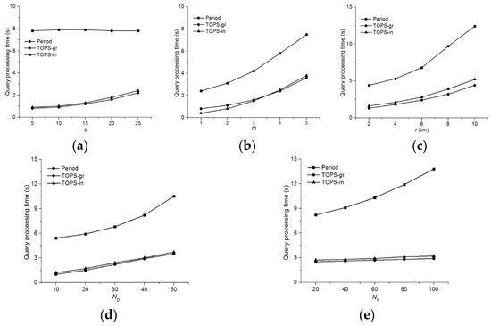
Figure 10.
Comparison of the query processing time for . (a) Effect of k; (b) Effect of m; (c) Effect of r; (d) Effect of ; (e) Effect of .
Figure 10c shows the comparison of query processing time of Period, and with different values of r. Experimental results reveal that the computational time increases under all of the algorithms as the range r increases. This is mainly because the search space increases in proportion to r. Figure 10d,e demonstrate the performance of Period, and with different values of ND and NF, respectively, which indicate that the query processing time of Period increases with the value of ND and NF because the Period method investigates all of the feature objects within the query range of each data object. and exhibited similar trends because both algorithms explore the pairs sequentially in the skyline sets in descending order based on the range score. However, scale better than due to grouping, which allows fewer pairs to investigate. It should be noted that according to Figure 10e, increasing NF has little impact on the performance of and because both and materializes the pairs that are dominant, and thus the number of pairs are not affected significantly by increasing NF.
Figure 11 shows the query processing time for and the Period method for the nearest neighbor condition. Figure 11a illustrates the effect of various values of k on the query processing time by all the algorithms, which shows that both and clearly outperforms the Period method, although the query processing time of Period is stable regardless of the k value. This is mainly because the Period method continues network expansion until the closest feature object is found for each data object. Figure 11b shows the query processing time as a function of the m value. The query processing times increases rapidly for all of the methods with the m value. However, and perform better than Period in all cases. Figure 11c shows the effect of the number of data objects on the query processing time of Period, and . Observe that all the three algorithms are sensitive towards the number of data objects, but significantly outperforms the Period, while is comparable to Figure 11d compares the query processing time of Period, and with different values of NF, which indicates that both and scale better than Period.
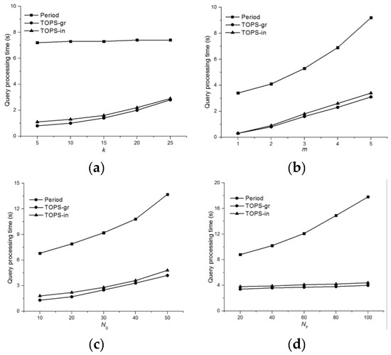
Figure 11.
Comparison of the query processing time for . (a) Effect of k; (b) Effect of m; (c) Effect of ; (d) Effect of .
Figure 12 shows the query processing times for and the Period method for the influence condition. Figure 12a illustrates the query processing time as a function of the value of k. According to Figure 11a, and clearly outperforms Period regardless of the value of k. As shown in Figure 12b, we varied the number of feature sets m, and the experimental results demonstrates that the query processing times increases for all three methods as the value of m increases. clearly outperforms in each case. Figure 12c shows the effect of r on the query processing time. Notice that the query processing times of all three algorithms are sensitive to the increase in the range r, because the search space increased. In Figure 12d,e, we illustrate the effects on the query processing time by varying ND and NF, respectively, which indicate that and are always faster than Period, irrespective of the values of ND and NF because both algorithms employ materialized skyline sets.
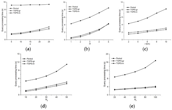
Figure 12.
Comparison of the query processing time for . (a) Effect of k; (b) Effect of m; (c) Effect of r; (d) Effect of ; (e) Effect of .
6.3. Experimental Results for Materialization and Incremental Maintenance Costs
In this section, we only present a performance comparison of and because the baseline method does not use any materialization and incremental maintenance scheme. Figure 13 shows an index construction time for and for various cardinalities of data and feature objects. The index construction time of both methods increased with the values of and . This is mainly because the number of pairs to be indexed increases with and . However, due to the grouping technique performs better for all cases.
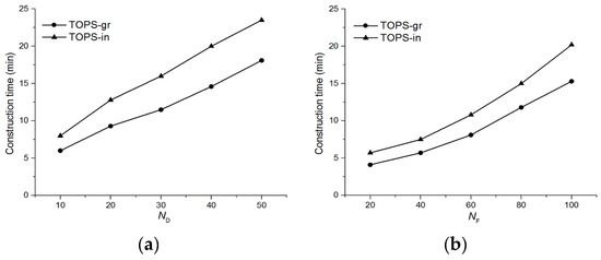
Figure 13.
Index construction time. (a) Effect of ; (b) Effect of .
In Figure 14, we study the effect of number of data objects and feature objects on the index size of and As shown in Figure 14a,b, the index size increased by increasing number of data and feature objects, respectively. However, consumed much less space as compared to because of the grouping technique which reduces the number of pairs to index.
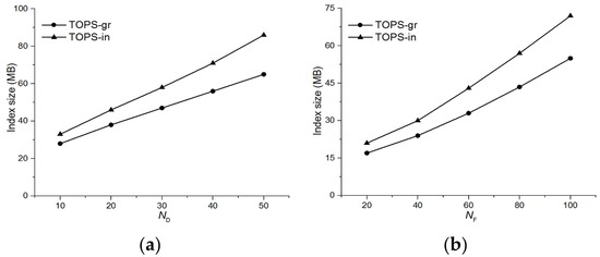
Figure 14.
Index size. (a) Effect of ; (b) Effect of .
Figure 15 shows comparisons of the average elapsed times for inserting a data object and deleting a feature object. In order to measure these times, both insertion of data objects and deletion of feature objects have been conducted 500 times, during which all other parameters remain the same. As shown in Figure 15, the maintenance time for is slightly longer than because, as mentioned in Section 5, first is updated and then is updated accordingly. Experimental results in Figure 15a depict that insertion time for a data object is not significantly affected by the number of data objects. This is because the leading factor for insertion time is generation of a dominant pair of new data objects which are the same regardless of the number of data objects. The only factor that causes the slight increase in insertion time is the update of the materialized dominant set which increases with the value of . Figure 15b shows that deletions of feature objects are more expensive than insertions of data objects and the average deletion time of a feature object is sensitive to the number of feature objects. This is mainly because the number of pairs that are exclusively dominated by deleted feature object pairs increases with . Thus, the dominance sets for more new pairs are determined resulting in an increase in time.
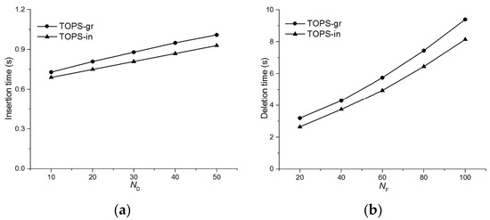
Figure 15.
Incremental maintenance cost. (a) Effect of on insertion time of data object; (b) Effect of on deletion time of feature object.
6.4. Comparison of TOPS and ALPS+
In this section, we present a performance comparison of TOPS and ALPS+. Note that in this section TOPSgr is referred as TOPS. As discussed earlier ALPS is originally designed for processing preference queries in undirected road networks. To make a fair comparison, we modified ALPS to process top-k spatial preference queries in directed road networks which we call ALPS+. Specifically, we perform two major modifications; firstly, we assume that only data objects that resides in a bidirectional adjacent edges can be grouped together to create a data segment, and, secondly, we modified the technique for computing distance between data segments and feature objects.
Figure 16 shows the performance of query processing times of TOPS and for the range condition. Figure 16a studies the effect of k on query processing time of TOPS and whereas Figure 16b shows the effect of r on performance of both algorithms. The experimental results reveal that the query processing time of both methods increases with the value of k and r. However, TOPS clearly outperforms in each case because the number of data and feature objects pairs in is higher than TOPS. The main reason is that first groups the data objects then prunes the pairs based on the dominance relation which may include the redundant pairs. Whereas, our proposed method first prunes the dominated pairs and then groups them to remove any redundant pairs.
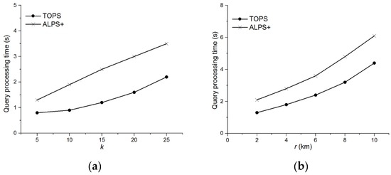
Figure 16.
Comparison of TOPS and for (a) Effect of k on query processing time; (b) Effect r on query processing time.
7. Conclusions
In this paper, we studied top-k spatial preference queries in directed road networks. We proposed a new approach called TOPS to enhance the performance of top-k spatial preference queries in directed road networks. Our approach is based on the pruning and grouping of feature objects, thereby minimizing the number of subsets of pairs required to rank the data objects. Skyline pairs that are not dominated by other pairs are mapped onto the distance-score space, and a skyline set is then generated and indexed in an R-tree. To achieve this, we presented mathematical formulae for determining the minimum and maximum distances between a data object and a feature group. Furthermore, we proposed an efficient algorithm for processing top-k spatial preference queries while ensuring materialized information is updated.
For experimental evaluation, we implemented two versions of TOPS: and and compared them with the Period approach. To be precise, uses materialized data and feature group pairs whereas uses the materialized data and feature object sets. Based on our experimental findings, both and significantly outperform the Period approach in terms of query processing time for various parameters. However, both and are comparable in terms of query processing time; but is superior in terms of materialization costs.
Acknowledgments
We thank anonymous reviewers for their valuable comments and suggestions. Muhammad Attique, Rize Jin and Tae-Sun Chung were supported by Basic Science Research Program through the National Research Foundation of Korea (NRF) funded by the Ministry of Education (2013R1A1A2A10012956 and NRF-2012R1A1A2043422). Hyung-Ju Cho was supported by the National Research Foundation of Korea (NRF) grant funded by the Korean government (MSIP) (No. NRF-2016R1A2B4009793). Finally, this work was partially supported by the Ajou University research fund.
Author Contributions
All authors significantly contributed to the manuscript. Muhammad Attique initiated the idea, implemented the experiments and wrote the manuscript. Muhammad Attique and Hyung-Ju Cho designed the solution and experiments. Hyung-Ju Cho critically reviewed the paper and revised the manuscript. Tae-Sun Chung and Rize Jin reviewed the manuscript and supervised the research.
Conflicts of Interest
The authors declare no conflict of interest.
References
- Bao, J.; Chow, C.; Mokbel, M.; Ku, W. Efficient evaluation of k-range nearest neighbor queries in road networks. In Proceedings of the Eleventh International Conference on Mobile Data Management (MDM), Kansas City, MO, USA, 23–26 May 2010; pp. 115–124.
- Cho, H.-J.; Ryu, K.-Y.; Chung, T.-S. An efficient algorithm for computing safe exit points of moving range queries in directed road networks. Inf. Syst. 2014, 41, 1–19. [Google Scholar] [CrossRef]
- Cheema, M.; Lin, X.; Zhang, Y.; Zhang, W.; Li, X. Continuous reverse k nearest neighbors queries in Euclidean space and in spatial networks. VLDB J. 2012, 21, 69–95. [Google Scholar] [CrossRef]
- Attique, M.; Hailu, Y.; Gudeta, S.; Cho, H.-J.; Chung, T.-S. A safe exit approach for continuous monitoring of reverse k-nearest neighbors in road networks. Int. Arab J. Inf. Technol. 2015, 12, 540–549. [Google Scholar]
- Wang, H.; Zimmermann, R. Processing of continuous location-based range queries on moving objects in road networks. IEEE Trans. Knowl. Data Eng. 2011, 23, 1065–1078. [Google Scholar] [CrossRef]
- Ilyas, I.; Beskales, G.; Soliman, M. A survey of Top-k query processing techniques in relational database systems. ACM Comput. Surv. 2008, 40. [Google Scholar] [CrossRef]
- Mamoulis, N.; Yiu, M.; Cheng, K.; Cheung, D. Efficient Top-k aggregation of ranked inputs. ACM Trans. Database Syst. 2007, 32. [Google Scholar] [CrossRef]
- Yiu, M.; Lu, H.; Mamoulis, N.; Vaitis, M. Ranking spatial data by quality preferences. IEEE Trans. Knowl. Data Eng. 2011, 23, 433–446. [Google Scholar] [CrossRef]
- Yiu, M.; Dai, X.; Mamoulis, N.; Vaitis, M. Top-k spatial preference queries. In Proceedings of the IEEE 23rd International Conference on Data Engineering (ICDE 2007), Istanbul, Turkey, 15–20 April 2007.
- Rocha-Junior, J.; Vlachou, A.; Doulkeridis, C.; Nørvag, K. Efficient processing of top-k spatial preference queries. PVLDB 2010, 4, 93–104. [Google Scholar] [CrossRef]
- Cho, H.-J.; Kwon, S.-J.; Chung, T.-S. ALPS: An efficient algorithm for top-k spatial preference search in road networks. Knowl. Inf. Syst. 2015, 42, 599–631. [Google Scholar] [CrossRef]
- Attique, M.; Qamar, R.; Cho, H.-J.; Chung, T.-S. A new approach to process top-k spatial preference queries in a directed road network. In Proceedings of the Third ACM SIGSPATIAL International Workshop on Mobile Geographic Information Systems, Dallas, TX, USA, 4–7 November 2014.
- Kolahdouzan, M.; Shahabi, C. Voronoi-based k nearest neighbor search for spatial network databases. In Proceedings of the Thirtieth International Conference on Very Large Data Bases, Toronto, ON, Canada, 31 August–3 September 2004.
- Song, Z.; Roussopoulos, N. k-Nearest neighbor search for moving query point. In Proceedings of the 7th International Symposium on Advances in Spatial and Temporal Databases, Redondo Beach, CA, USA, 12–15 July 2001.
- Sun, Y.; Yu, X.; Bie, R.; Song, H. Discovering time-dependent shortest path on traffic graph for drivers towards green driving. J. Netw. Comput. Appl. 2016, in press. [Google Scholar] [CrossRef]
- Lin, Q.; Zhang, Y.; Zhang, W.; Lin, X. Efficient general spatial skyline computation. World Wide Web 2013, 16, 247–270. [Google Scholar] [CrossRef]
- Lee, K.; Zheng, B.; Chen, C.; Chow, C. Efficient Index-based approaches for skyline queries in location-based applications. IEEE Trans. Knowl. Data Eng. 2013, 25, 2507–2520. [Google Scholar] [CrossRef]
- Liu, W.; Jing, Y.; Chen, K.; Sun, W. Combining top-k query in road networks. In Web-Age Information Management; Springer: Berlin, Germany, 2012; pp. 63–75. [Google Scholar]
- Deng, K.; Zhou, X.; Shen, H. Multi-source skyline query processing in road networks. In Proceedings of the IEEE 23rd International Conference on Data Engineering, Istanbul, Turkey, 15–20 April 2007.
- Chen, J.; Huang, J.; Jiang, B.; Pei, J.; Yin, J. Recommendations for two-way selections using skyline view queries. Knowl. Inf. Syst. 2013, 34, 397–424. [Google Scholar] [CrossRef]
- Wang, Y.; Wei, W.; Deng, Q.; Liu, W.; Song, H. An energy-efficient skyline query for massively multidimensional sensing data. Sensors 2016, 16. [Google Scholar] [CrossRef] [PubMed]
- Cheema, M.; Lin, X.; Zhang, W.; Zhang, Y. A safe zone based approach for monitoring moving skyline queries. In Proceedings of the 16th International Conference on Extending Database Technology, Genoa, Italy, 18–22 March 2013; pp. 275–286.
- Xia, T.; Zhang, D.; Kanoulas, E.; Du, Y. On computing top-t most influential spatial sites. In Proceedings of the 31st International Conference on Very Large Data Bases, Trondheim, Norway, 30 August–2 September 2005.
- Du, Y.; Zhang, D.; Xia, T. The optimal-location query. In Advances in Spatial and Temporal Databases; Springer: Berlin, Germany, 2005; pp. 163–180. [Google Scholar]
- Zhang, D.; Du, Y.; Xia, T.; Tao, Y. Progessive computation of the min-dist optimal-location query. In Proceedings of the 32nd International Conference on Very Large Data Bases, Seoul, Korea, 12–15 September 2006.
- Mouratidis, K.; Lin, Y.; Yiu, M. Preference queries in large multi-cost transportation networks. In Proceedings of the 2010 IEEE 26th International Conference on Data Engineering (ICDE 2010), Long Beach, CA, USA, 1–6 March 2010.
- Lin, P.; Yin, Y.; Nie, P. K-multi-preference query over road networks. Pers. Ubiquitous Comput. 2016, 20, 413–429. [Google Scholar] [CrossRef]
- Hartmann, A. Phase Transitions and Clustering Properties of Optimization Problems; Lecture given at DPG Physics School: Bad Honnef, Germany, 2012. [Google Scholar]
- Guttman, A. R-Trees: A dynamic index structure for spatial searching. In Proceedings of the 1984 ACM SIGMOD international conference on Management of data, Boston, MA, USA, 18–21 June 1984.
- Real Datasets for Spatial Databases. Available online: http://www.cs.fsu.edu/~lifeifei/SpatialDataset.htm (accessed on 13 October 2014).
- American Hotel & Lodging Association. Available online: http://www.ahla.com/ (accessed on 4 August 2015).
- Papadias, D.; Zhang, J.; Mamoulis, N.; Tao, Y. Query processing in spatial network databases. In Proceedings of the 29th International Conference on Very Large Data Bases, Berlin, Germany, 9–12 September 2003; pp. 802–813.
- Dijkstra, E. A note on two problems in connexion with graphs. Numer. Math. 1959, 1, 269–271. [Google Scholar] [CrossRef]
© 2016 by the authors; licensee MDPI, Basel, Switzerland. This article is an open access article distributed under the terms and conditions of the Creative Commons Attribution (CC-BY) license (http://creativecommons.org/licenses/by/4.0/).