Pattern of Spatial Distribution and Temporal Variation of Atmospheric Pollutants during 2013 in Shenzhen, China

Abstract

Air pollution caused by atmospheric particulate and gaseous pollutants has drawn broad public concern globally. In this paper, the spatial-temporal distributions of major air pollutants in Shenzhen from March 2013 to February 2014 are discussed. In this study, ground-site monitoring data from 19 monitoring sites was used and spatial interpolation and spatial autocorrelation methods were applied to analyze both spatial and temporal characteristics of air pollutants in Shenzhen City. During the study period, the daily average concentrations of Particulate Matter (PM₁₀ and PM_2.5) ranged from 16–189 μg/m³ and 10–136 μg/m³, respectively, with 13 and 44 over-limit days, indicating that particulate matter was the primary air pollutant in Shenzhen. The highest PM occupation in the polluted air was observed in winter, indicating that fine particulate pollution was most serious in winter. Meanwhile, seasonal agglomeration patterns for six kinds of air pollutants showed that Guangming, Baoan, Nanshan, and the northern part of Longgang were the most polluted areas and PMs were their primary air pollutants. In addition, wind scale and rainfall played an important role in dissipating air pollutant in Shenzhen. The wind direction impacted the air pollution level in Shenzhen in multiple ways: the highest concentrations for all air pollutants all occurred on days with a northeast wind; the second highest ones appeared on the days with no wind. The concentrations on days with north-related winds are higher on average than those of days with south-related winds.

1. Introduction

Air pollution has always been an inevitable and non-negligible global issue accompanied by the economic development and technological advancement of human society, especially in China. The assessment of urban air quality and pollution control has become one of the major subjects in the field of atmospheric pollution research [1]. In recent years, a remarkable effort has been made to investigate the mechanisms, sources, compositions, and patterns of air pollution (especially Particulate Matter (PM) pollution) in China, mostly focusing on a few mega-cities and major regions, such as Beijing, Shanghai, Guangzhou, the Jing-Jin-Ji region, and the Pearl River Delta region. Among these studies, some have focused on the chemical composition or source apportionment of air pollutants [2,3,4,5]; others have attempted to reveal the spatial and temporal patterns of air pollutants, including the spatial distribution or the simulation of changing trends [6,7,8,9], the demonstration of temporal variation [10,11,12], and correlation analysis [13,14].

The Pearl River Delta (PRD) region is one of the most developed regions with the highest aggregation of industry in China. Severe air pollution has been observed on both urban and regional scales in this region, including high concentrations of particulate matter [15,16,17], nitrogen dioxide [18,19,20], and ozone [20,21], due to rapid urbanization and industrialization, as well as the increasing burden of local traffic. Shenzhen, located in the urban agglomeration of the PRD region, plays an important role in connecting Hong Kong and the inland PRD. Owing to its particular geographical position in the PRD region, the air quality in Shenzhen can reflect not only the regional characteristics of air pollution but also the regional transport between Hong Kong and the inland PRD to a certain degree [22]. Shenzhen was once praised as an Environmental Protection Model City in 1997 for its favorable air environment. However, with the continuous development of urbanization and industrialization in the PRD region, the air quality in Shenzhen has deteriorated gradually in the last few years. The increasing local industrial fuel consumption and rising number of vehicles (the vehicle amount had exceeded three million by the end of 2014 with the highest traffic density in China) have generated high levels of air pollutants, which are responsible for the degradation of atmospheric visibility and frequent hazy weather [23]. Therefore, it is significant to understand the state of air pollution in Shenzhen where the air quality has deteriorated in recent years. Meanwhile, studies on air pollution in Shenzhen can also contribute to a better understanding of the regional correlation between air pollution in Hong Kong and the inland PRD region. In this study, we used ground-site monitoring data from 19 monitoring sites spread over the whole city area to analyze both spatial and temporal characteristics of air pollutants in Shenzhen. We intend to investigate the major air pollutants and reveal the seasonal variation of major pollutants and the agglomeration patterns of major pollutants by identifying hot spots and cold spots, as well as the key areas for taking measures specific to one certain air pollutant.

The remainder of the paper is organized as follows. The data and methods are described in Section 2. After the overall condition of air quality in Shenzhen is described in Section 3.1, we focus further on seasonal variations of air pollutants and pollution levels in Section 3.2. In Section 3.3, we identify the spatial agglomeration pattern of each air pollutant and further evaluate the regional air quality and pollution level in different seasons. Discussion is also presented in these sections and, finally, conclusions are drawn in Section 4.

2. Materials and Methods

2.1. Data Collection

The ground-site monitoring data was supplied by the Shenzhen environmental monitoring center. The monitoring network is composed of 19 ground-based monitoring sites scattered around the entire study area (Figure 1). All of the monitoring sites are equipped with a global positioning system (GPS) and instruments for continuous real-time monitoring of several kinds of air pollutants, including PM_2.5, PM₁₀, CO, SO₂, O₃, and NO₂. It can provide a great quantity of samples for all kinds of studies in the field of atmospheric pollutants. The TEOM 1405-F instrument (Thermo Fisher Scientific Inc., Waltham, MA, USA) was used to detect the mass concentration of PM₁₀ using filters and an oscillating microbalance with a flow rate of 16.7 L/min. The 5030i SHARP instrument (Thermo Fisher Scientific Inc., Waltham, MA, USA) was used to detect the mass concentration of PM_2.5 using β-ray detection with a flow rate of 16.7 L/min. PM_2.5 was first included in the monitoring system in Shenzhen in 2013; therefore, we chose the period from March 2013 to February 2014 for study. In this study, the daily-averaged mass concentrations (maximum within eight hours for O₃) of the six air pollutants were collected at each site from March 2013 to February 2014. Excluding days with instrument failure, efficacious (successful observations for all six air pollutants on 80% sites or more) monitoring samples were obtained on 349 days: 83, 89, 90, and 87 monitoring days in spring, summer, fall, and winter, respectively.

2.2. Mathematical Measures

On account of the pollution level at each site may have certain differences, the daily average concentration of all monitoring sites was acquired by applying a centering method (Equation (1)) supported by the Pollution and Health: a European Approach project [6]:

$$X_t=\frac{{{\displaystyle \sum }}_{i=1}^n\left[\left(X_{it}-X_i\right)\right]}{n}+X$$

(1)

where $X_t$ is the average mass concentration of all sampling sites (n) on the t-th day, $X_{it}$ is the mass concentration of the i site on the t-th day, $X_i$ is the average mass concentration of the i site during the sampling period, and X is the average mass concentration of all sites during the sampling period.

In addition, we used the air quality index (AQI) to evaluate the air quality in Shenzhen. In March 2012, the Chinese Ministry of Environmental Protection (MEP) released the official revisions of the ambient air quality index (AQI), which were calculated based on six pollutants, including SO₂, NO₂, PM_2.5, PM₁₀, CO, and O₃ (8 h peak) [24]. The AQI was proposed to evaluate the pollution level of the air and adverse effects on human body after a long-term exposure in the polluted air. AQI applied the concept of transferring the mass concentrations of six air pollutants into one unified standard level (Equation (2)), namely the individual air quality index (IAQI). AQI, defined as the maximum value of the six IAQIs (Equation (3)), is a non-dimensional indicator focusing on one single air pollutant. When AQI is larger than 50, the air pollutant whose IAQI is the maximum is considered to be the major pollutant. When IAQI is larger than 100, the corresponding air pollutant is classified as a standard-exceeded pollutant. In this study, IAQIs also were employed in investigating the composition proportion of each air pollutant.

$$I_P=\frac{I_{Ph}-I_{Pl}}{C_{Ph}-C_{Pl}}\left(C_P-C_{Pl}\right)+ I_{Pl}$$

(2)

where $C_{Ph}$ and $C_{Pl}$ represent the high-value and low-value of the concentration interval where $C_P$ belongs, respectively; $I_{Ph}$ and $I_{Pl}$ represent the values of IAQI corresponding to $C_{Ph}$ and $C_{Pl}$, respectively, in Appendix A.

$$\mathrm{AQI}=\max \left\{{\mathrm{IAQI}}_1,{\mathrm{IAQI}}_2,{\mathrm{IAQI}}_3,\dots ,{\mathrm{IAQI}}_n\right\}$$

(3)

2.3. Kriging Interpolation

Collected air pollutant concentrations were limited by locations of the monitoring sites, which cannot represent an integrated spatial pattern of pollution over the whole study area. While it is impractical to add more sampling sites, spatial interpolation can provide an efficient way of generating a complete spatial pattern of attribute with fine resolution in a large range. Kriging interpolation is a geostatistical technique to estimate values at unmeasured locations based on empirical spatial structure quantified in a semivariogram model [25]. In this study, concentrations of all air pollutants across the whole study area were obtained by applying ordinary kriging interpolation.

Ordinary kriging (OK), known as the most common type of kriging in practice, is a local optimal linear unbiased estimation method. It is a powerful tool for characterizing spatial pattern of attributes with spatial continuity, widely applied in the research fields of soil, precipitation, underground water, atmospheric studies, and so on [26,27,28]. The estimate of variable $Z$ at location $s_0$, $\widehat{Z}\left(s_0\right)$ is a linear weighted sum of n observations surrounding the predicted location:

$$\widehat{Z}\left(s_0\right)= {\displaystyle \sum }_{i=1}^N{\lambda }_{i}Z\left(s_i\right)$$

(4)

where $Z\left(s_i\right)$ is the observed value of location i, ${\lambda }_i$ is the weight of the observed value at location i, $s_0$ is the predicted location, and $N$ is the number of observed values.

The $N$ weights are determined on the principle that the estimate is unbiased and has minimum kriging variance. The unbiasedness can be ensured by making the sum of $N$ weights equal to 1. A detailed theoretical description of the kriging algorithms was provided by Webster and Oliver [29].

2.4. Spatial Autocorrelation

Spatial autocorrelation is a spatial analysis method based on the First Law of Geography [30] in which all objects on a geographic surface are related to each other with special consideration of distance and closer ones are more related than distant ones. It is identified as three kinds of patterns (clustered, random, or regular) in spatial autocorrelation, which can be measured by Moran’s I [31,32]. Moran’s I generally refers to Global Moran’s I (GMI), which provides a comprehensive evaluation of the spatial autocorrelation. Correspondingly, there is a Local Moran’s I (LMI) [33]. GMI is used to evaluate the degree of spatial concentration of the whole study area, while LMI is used to explore the spatial distribution of the “hot spots” and “cold spots” at a local scale. In the field of atmospheric study, considering the spatial correlation properties of atmospheric activity, spatial autocorrelation is proven to be a powerful tool to reveal the potential spatial pattern for observed data within the distributed area, providing theoretical foundations for exploring spatial agglomeration and evolution patterns for air pollution [7,34]. Both GMI and LMI were applied in this study to characterize the global and local aggregation patterns of pollutant concentrations. GMI is defined as:

$$I=\frac{n}{S_0}\times \frac{{{\displaystyle \sum }}_{i=1}^n{{\displaystyle \sum }}_{j=1}^n{w}_{ij}\left(x_i-\overline{x}\right)\left(x_j-\overline{x}\right)}{{{\displaystyle \sum }}_{i=1}^n{\left(x_i-\overline{x}\right)}^2}$$

(5)

LMI refers to:

$$I_i=\frac{\left(x_i-\overline{x}\right)}{S_i^2}{\displaystyle \sum }_{j=1, \ne i}^n{w}_{ij}\left(x_j-\overline{x}\right)$$

(6)

where n is the total number of the sample, $x_i$ and $x_j$ are the pollutant concentration in locations of i and j, respectively; $\overline{x}$ is the average value for a location; $w_{ij}$ is the spatial weight matrix (n × n), it represents the spatial neighbor relationship of location i and location j (1: adjacent, 0: not adjacent)

$$S_0={\displaystyle \sum }_{i=1}^n{\displaystyle \sum }_{j=1}^n{w}_{ij}$$

(7)

$$S_i^2={\displaystyle \sum }_{j=1, j\ne i}^n{w}_{ij}/\left(n-1\right)-{\overline{x}}^2$$

(8)

The significance test of Moran’s I can be measured by the standardized statistics $Z$ test, which is defined as:

$$Z_I= \frac{I-E\left(I\right)}{SD\left(I\right)}$$

(9)

where $E\left(I\right)= -1/\left(n-1\right)$ for GMI; $E\left(I\right)= -{\displaystyle \sum }_{j=1, j\ne i}^n{w}_{ij}/\left(n-1\right)$ for LMI, $SD\left(I\right)$ is the standard deviation of I.

The higher the absolute value of $Z$ (>1.65), the stronger the intensity of the clustering will be. A positive $Z$ value implies agglomeration of high values, namely a “hot spot”; a negative $Z$ value implies agglomeration of low values, namely a “cold spot”. A $Z$ value around zero indicates no significant clustering pattern. In this study, the spatial autocorrelation was employed to investigate the spatial pattern and extract hot-spots of air pollutant concentrations.

3. Results and Discussion

3.1. Overview

We calculated the annual averages and daily averages of collected concentrations from all monitoring sites for six air pollutants. As shown in

Table 1. Statistics of annual average and daily average concentrations for air pollutants in Shenzhen from March 2013 to February 2014 (mg/m³ for CO, μg/m³ for others).

Air Pollutant	Annual Average	Annual Average Limit		Daily Average Limit	Days over Limit
		Class I	Class II
SO2	13	20	60	150	0
NO2	39	40	40	80	6
CO	1.18			4	0
O3 8h	70			160	21
PM10	85	40	70	150	13
PM2.5	43	15	35	75	44

, the annual average concentrations of SO₂ and NO₂ were 13 and 39 μg/m³, respectively, both below the Chinese ambient air quality standards [35]. The annual average concentrations of CO and O₃ were 1.18 and 70 μg/m³, respectively. There is no standard for the annual average for these two air pollutants. The annual average concentrations of PM₁₀ and PM_2.5 were 85 and 43 μg/m³, respectively, both over the Chinese ambient air quality standards, making particulate matter the main air contaminant in this region. Nevertheless, the polluting level of particulate matters in Shenzhen was still lower than most mega-cities in China [14,36,37]. In 2013, the average concentration of PM_2.5 was 53 μg/m³ in Guangzhou, 87.81 μg/m³ in Beijing, 103.07 μg/m³ in Shanghai (62.25 μg/m³ in the Putuo district), and 114.88 μg/m³ in Nanjing.

Considering the daily average concentration, SO₂ and CO met the primary standard with respect to Chinese ambient air quality standards. Therefore, this study primarily focused on the other four standard-exceeding air pollutants. Concentration variations of the four air pollutants throughout the entire study period are represented in Figure 2 and Figure 3. Daily average concentrations of NO₂ ranged from 14–105 μg/m³, with six over-limit days occurring in spring and winter. Daily average concentrations of O₃ ranged from 19–207 μg/m³, with 21 over-limit days mostly occurring in summer and autumn. Daily average concentrations of PM₁₀ and PM_2.5 ranged from 18–189 μg/m³ and 10–136 μg/m³, respectively, with 13 and 44 over-limit days mostly occurring in winter. These variations implied certain associations among different air pollutants. Therefore, correlation tests were carried out to evaluate the coefficient of association between each pair of air pollutants. The correlation results showed that there was a significant correlation between PM₁₀ and PM_2.5 (R² = 0.92, p < 0.01). Both NO₂ and O₃ were marginally correlated with particulate matters, primarily PM₁₀ (R² = 0.52 for NO₂, R² = 0.57 for O₃, p < 0.01).

3.2. Seasonal Variation

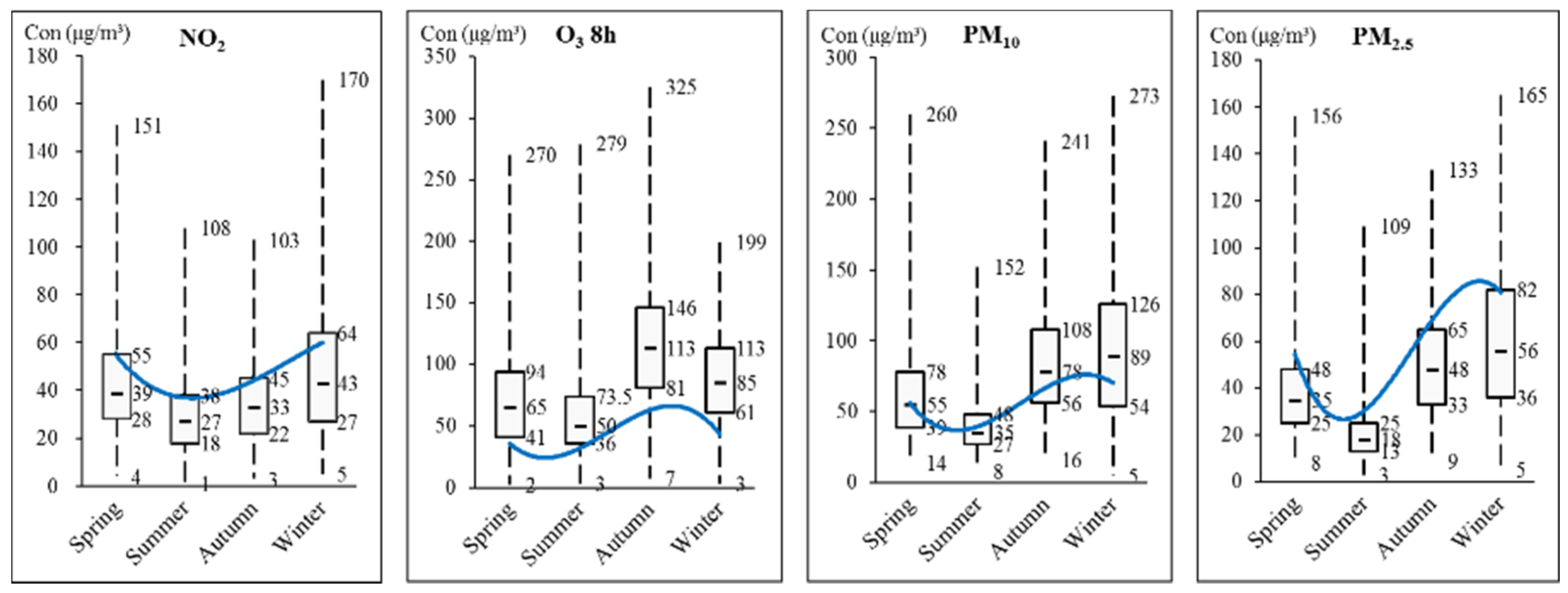
3.2.1. Variation of a Single Air Pollutant

In order to investigate the seasonal variation pattern of each air pollutant, the seasonal average and quartile (minimum, 25% quartile, 50% quartile, 75% quartile, and maximum) concentrations were calculated and are displayed in

Table 2. Seasonal average concentrations for air pollutants in Shenzhen from March 2013 to February 2014 (mg/m³ for CO, μg/m³ for others).

Season	NO2	O3 8h	PM10	PM2.5
Spring	54	36	56	54
Summer	37	32	40	30
Autumn	44	63	67	69
Winter	60	43	70	81

and Figure 4. For NO₂, the highest value appeared in winter with a seasonal average of 60 μg/m³ and the averaged concentration levels ranked from highest to lowest as: winter, spring, autumn, and summer. For O₃, the highest value appeared in autumn with a seasonal average of 63 μg/m³ and the averaged concentration levels ranked as: autumn, winter, spring, and summer. For PM₁₀ and PM_2.5, the highest values both appeared in winter with a seasonal average of 70 and 81 μg/m³, respectively, and the averaged concentration levels ranked consistently as: winter, autumn, spring, and summer.

Compared with Figure 2 and Figure 3, there were few discrepancies in the seasonal variation trends in Figure 4, e.g., the highest concentration of O₃ which appeared in July in Figure 3 was observed in autumn in Figure 4. That was because the data used for generating the year-round variation curve was averaged by the 19 monitoring sites while the data used for the quartile calculation was based on single monitoring sites for each air pollutant. In this way, the significance of extreme values can be retained integrally.

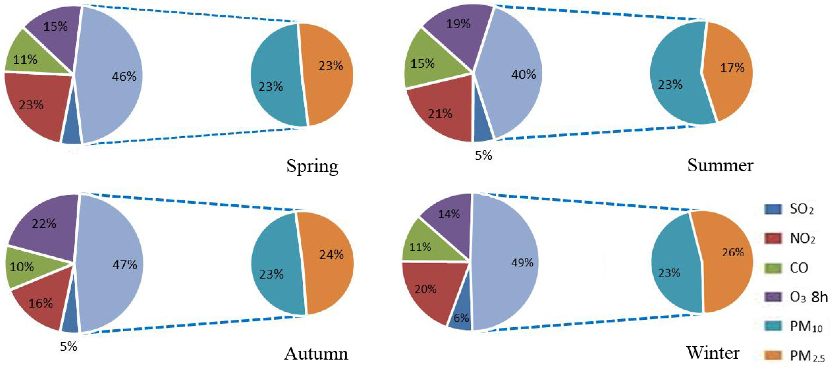
3.2.2. Variation of Air Pollutant Levels

On the basis of understanding the seasonal variation patterns of single air pollutants, it was necessary to evaluate the air pollution level comprehensively. For the purpose of evaluating the air pollution level, monthly-averaged AQI and relevant IAQIs were calculated for each month during the study period (

Table 3. Monthly AQI and IAQIs for air pollutants in Shenzhen from March 2013 to February 2014.

Season	Month	AQI	I-SO2	I-NO2	I-CO	I-O3	I-PM10	I-PM2.5
Spring	3	63	13	62	27	39	63	61
	4	64	13	55	27	39	61	64
	5	46	10	46	27	29	44	38
Summer	6	38	9	34	29	30	38	30
	7	34	8	33	25	28	34	24
	8	47	10	44	26	38	47	37
Autumn	9	55	9	40	26	50	55	51
	10	91	16	47	34	91	78	89
	11	68	14	46	30	48	67	68
Winter	12	105	25	69	38	50	83	105
	1	89	19	67	36	42	77	89
	2	51	12	44	31	38	51	50

). According to the Ministry of Environmental Protection of the People’s Republic of China [24], the classification of the AQI is as follows: when the AQI lies between 0 and 50, it implies that the air quality is favorable and the air environment is hardly polluted; when the AQI lies between 51 and 100, it implies that the air quality is acceptable and it may generate a weak influence on susceptible populations; when the AQI lies between 101 and 150, it implies that the air environment is mildly polluted and it may cause adverse effects on healthy populations. In terms of the air environment in Shenzhen, the air quality was favorable from May–August with AQI values lying under 50; December was the most polluted month with an AQI exceeding 100. On the whole, the air quality was favorable in summer, acceptable in spring and autumn, and mildly polluted in winter. From the seasonal air pollutant composition graph in Figure 5 we can see that NO_2, O₃, and PMs were the main constituents in the polluted air; the higher the pollution level, the greater the percentage PMs accounted for. In the meantime, PM_2.5 accounted for greater percentages than PM₁₀ in winter and lower percentages in summer, indicating that fine particulate (PM_2.5) pollution was more serious in winter, which was also in accordance with some relevant findings in other studies [6,13,37]. Seasonal variations in PMs in Shenzhen were probably caused by meteorological conditions of a typical monsoon climate [38,39]. In summer, the PM concentration levels were quite low due to the prevailing wind from the sea with clean air masses, while severe PM pollution occurred in winter, caused by the prevailing wind from the inland PRD with polluted air masses. The wind rose for each season in Shenzhen during the study period is shown in Figure 6.

3.3. Spatial-Temporal Pattern

Viewed from the overall angle, annual and seasonal average concentrations of air pollutants from the entire Shenzhen area were maintained at a relatively low level. It is necessary to dig up further characteristics of these air pollutants from a spatial perspective. Quantifying the spatial patterns of air pollution for a long period of time in an urban area is essential for investigating the air environmental quality in this area.

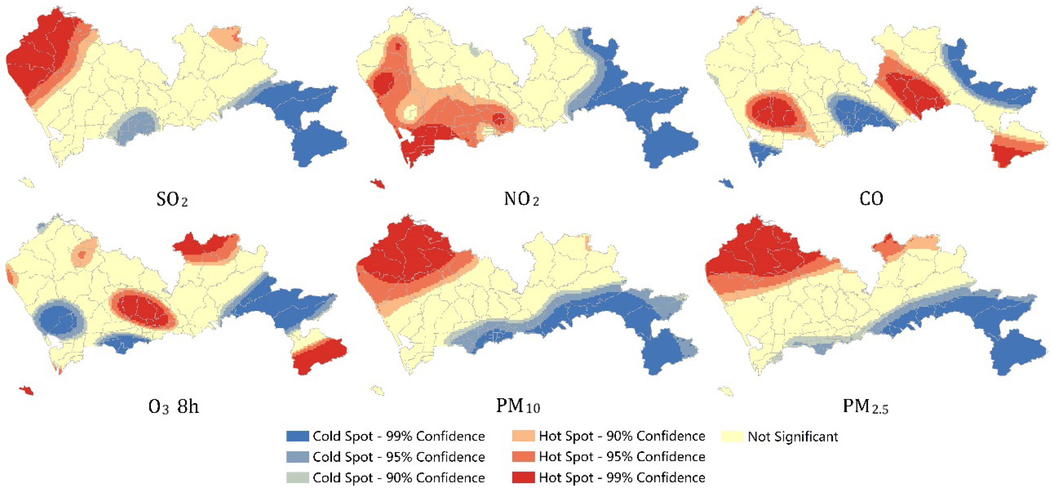
3.3.1. Spatial Agglomeration of Single Air Pollutants

Intensive air pollutant concentration distributions (1 km grid) covering the whole city were generated by applying kriging interpolation for air pollutants. Spatial autocorrelation analysis was then carried out for evaluating the global autocorrelation and generating agglomeration patterns for each air pollutant. The Global Moran’s I for each air pollutant indicated a high global clustered autocorrelation in this area, while the Local Moran’s I represented high-high and low-low clustering patterns for each air pollutant (Figure 7).

For SO₂, high concentrations were mostly aggregated in the northwestern area of Shenzhen (Guangming, northern part of Baoan) while low concentrations were aggregated in the southern and eastern parts of Shenzhen (Dapeng and Futian). The main source of SO₂ in urban cities is usually emissions from factories. For NO₂, high concentrations were aggregated in the southwestern area of Shenzhen (Baoan, Nanshan, and Futian), while low concentrations were aggregated in the eastern area of Shenzhen (Dapeng and Pingshan). Relevant research found out that the local traffic volume had a significant influence on the concentration level of NO₂ [10].

For CO, high concentrations were mostly aggregated in Nanshan, Longgang, Yantian, and the southeastern part of Dapeng, while low concentrations appeared in Luohu, the eastern part of Pingshan, and the northern part of Dapeng. For O₃, high concentrations were mostly aggregated in the central area of Shenzhen (Longhua, Luohu, and Longgang), and the southeastern part of Dapeng, while low concentrations appeared in the western part of Shenzhen and the northern part of Dapeng. Concentrations of O₃ are mainly influenced by the solar radiation and the degree of exposure of the ground near the surface. Near-surface pollutant O₃, which has no significant relationship with the ozone layer in the upper atmosphere, usually comes from human activities and industrial production in urban cities. Related research has found that the products of chemical reactions of NO₂ and volatile organic compounds play an important role in affecting the pollution level of O₃ in this area [40]. Moreover, when the air is severely polluted by PMs, the concentration of O₃ can be quite low thanks to the absorption and reflection by suspended particles.

For PMs, PM₁₀ and PM_2.5 presented similar patterns in spatial concentration agglomeration to SO₂. High concentrations were mostly aggregated in the northwestern area of Shenzhen (Guangming, northern part of Baoan), while low concentrations were aggregated in the southern and eastern parts of Shenzhen (Dapeng, Yantian, Luohu, and Futian). Relevant research showed that PMs were more associated with local sources, regional transport, and meteorological conditions [22,23]. All in all, the spatial distribution of air pollutants can be influenced by several complicated factors which require further investigation.

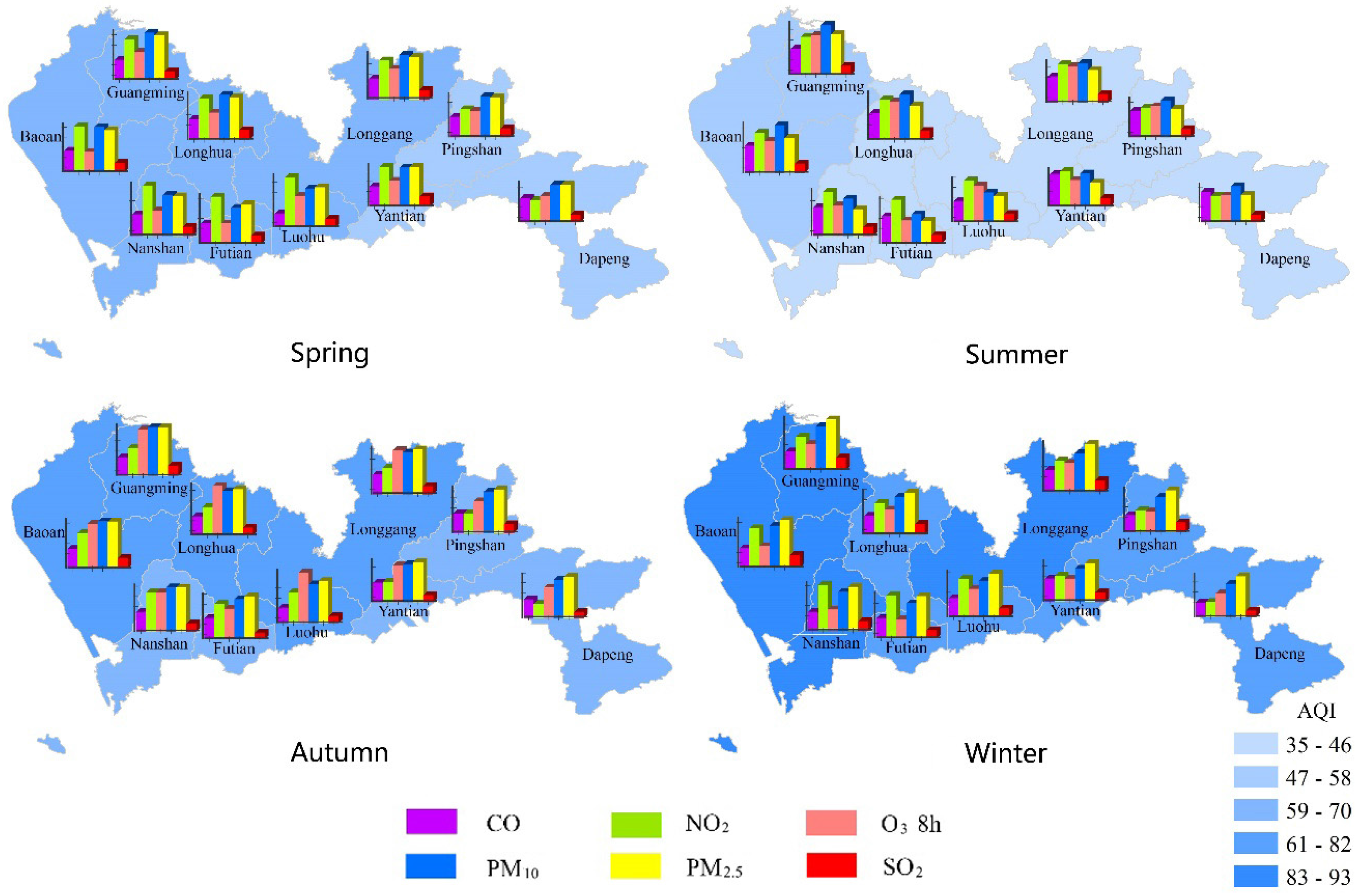
3.3.2. Regional Air Quality and Pollution Levels

On the basis of understanding the spatial patterns of single air pollutants, regional air quality and pollution levels were further evaluated comprehensively in this section. Shenzhen is divided into 10 administrative districts. Seasonal AQI and relevant IAQIs were calculated for each district (Figure 8 and Figure 9).

In Figure 8, Guangming, Baoan, and Nanshan ranked in the top three, with respect to the sum of AQIs for all seasons, and, therefore, they were the most polluted areas in Shenzhen during the study period. Seasonal compositions of six air pollutants were represented in each district in Figure 9. Significant distinctions were found in both spatial and temporal distributions.

In spring, NO₂ and PMs accounted for quite large proportions of the air pollution in most districts, except for the eastern area (Dapeng and Pingshan) where the pollution level of NO₂ was relatively low. In districts with a dense population, e.g., Nanshan, Futian, Luohu, and Baoan, the pollution level of NO₂ was even higher than those of PMs. In summer, a significant decline of the proportions of PMs was recognized in the southern districts, while a slight growth in the proportion of O₃ was observed in Guangming, Longhua, and Luohu. The proportion of NO₂ was maintained at a relatively high level in most districts. In autumn, a significant growth in the proportion of O₃ was observed in the entire study area, especially in Luohu, Longgang, and Longhua, where O₃ exceeded the PMs in proportion. Meanwhile, the proportions of PMs rebounded in some way and were maintained at a level which was similar to that in spring. The proportion of NO₂ reduced correspondingly as the proportion of other pollutants increased. In winter, the proportion of O₃ declined to quite a low level, while proportions of NO₂ and PMs rose again. In the northern and eastern districts, PM_2.5 absolutely accounted for the highest proportion, while in the southwestern districts (Nanshan, Futian, and Luohu), both NO₂ and PM_2.5 represented an equal level of pollution to a certain extent. On the whole, Guangming, Baoan, Nanshan, and the northern part of Longgang were the most polluted areas and PMs were their primary air pollutants during the entire study period. In addition, NO₂ proportions were relatively high in Nanshan, Futian, Luohu, and the southern part of Baoan during spring and O₃ proportions were extremely high in Luohu, Longhua, and the northern part of Baoan in autumn.

3.4. Meteorological Correlation

In this section, we explored the relationship between air pollutants and meteorological factors (wind scale, rainfall, and wind direction) in Shenzhen during the study period. The entire study period was classified into several categories in terms of meteorological conditions. Then average concentrations of those days in each category were calculated for all six air pollutants. The classified average concentrations of six air pollutants are displayed in

Table 4. Air pollutant concentrations based on wind-scale classification in Shenzhen from March 2013 to February 2014 (mg/m³ for CO, μg/m³ for others).

Wind Scale	SO2	NO2	CO	O3 8h	PM10	PM2.5
0–3	13	43	1.10	82	64	42
4	10	33	1.06	73	55	35
5	9	25	0.74	74	53	33
6	7	24	1.02	72	47	33

and

Table 5. Air pollutant concentrations based on rainfall classification in Shenzhen from March 2013 to February 2014 (mg/m³ for CO, μg/m³ for others).

Rainfall	SO2	NO2	CO	O3 8h	PM10	PM2.5
0	17	51	1.18	103	88	58
0–10	11	38	1.07	80	58	38
10–25	8	37	0.99	49	35	24
25–50	7	36	0.98	38	26	18
50–100	6	35	0.97	50	33	22

. Table 4 represents the correlation between the air pollutants and wind scale in Shenzhen. We can see that, except for the CO at wind scale 6, all other concentration values decrease congruously as the wind scale increases. Table 5 represents the correlation between air pollutants and daily-average rainfall. It is obvious that average concentrations on rainy days are much lower than those on non-rainy days for all six air pollutants. Moreover, when the daily rainfall is below 50 mm, concentration values decrease congruously as the rainfall increase.

To explore how the wind direction correlated with air pollutants, all days in the study period were classified into eight categories in terms of eight wind conditions, north (N), northeast (NE), east (E), southeast (SE), south (S), southwest (SW), northwest (NW), and no wind (0). The classified results are represented in Figure 10. It is evident that the concentration values are the highest for all six air pollutants on the days with a northeast wind; the second highest concentration values appeared on the days with no wind. The concentration values on days with north-related winds are higher on average than those on days with south-related winds. The last finding is also in accordance with the seasonal variation caused by a monsoon climate.

In conclusion, meteorological factors are correlated with all six air pollutants in a significant way. For wind scale and rainfall, they play an important role in dissipating air pollutants in Shenzhen. For wind direction, different wind directions have different effects: generally, winds from the south have positive effects, while winds from north have negative effects on air pollution in Shenzhen.

4. Conclusions

The main purpose of this paper was to describe the spatial-temporal distribution of major air pollutants in Shenzhen from March 2013 to February 2014. According to the statistical results, PM₁₀ and PM_2.5 were the primary air contaminants in this region for the year, with annual average concentrations of 85 and 43 μg/m³, respectively. Daily average concentrations of PM₁₀ and PM_2.5 ranged from 16–189 μg/m³ and 10–136 μg/m³, respectively, with 13 and 44 over-limit days. Daily average concentrations of NO₂ and O₃ also exceeded the limitations on a number of days. Significant seasonal variations were captured for each air pollutant: for PMs and NO₂, higher concentrations were observed in winter, followed by autumn and spring; for O₃, higher concentrations were observed in autumn, followed by winter. Meanwhile, seasonal agglomeration patterns of air pollutants were generated by applying the kriging method and the spatial autocorrelation method. These patterns showed that Guangming, Baoan, Nanshan, and the northern part of Longgang were the most polluted areas and PMs were their primary air pollutants. Moreover, NO₂ pollution in Nanshan, Futian, Luohu, and the southern part of Baoan in spring and O₃ pollution in Luohu, Longhua, and the northern part of Baoan in autumn should also be issues worthy of concern.

In addition, meteorological factors are correlated with all six air pollutants in a significant way in Shenzhen. For wind scale and rain fall, they play an important role in dissipating air pollutants in Shenzhen. For wind direction, different wind directions have different effects: the concentration values are the highest for all six air pollutants on the days with a northeast wind; the second highest concentration values appeared on the days with no wind. The concentration values on days with north-related winds are higher on average than those on days with south-related winds.

However, air pollution is a complicated process influenced by comprehensive factors, including meteorology, human activities, topography, the surrounding circumstances, and so on. It will take more time and effort in further research to determine explicit interpretations for specific spatial-temporal patterns of air pollution. For instance, the southern part of Dapeng represented an exceptionally high level of O₃ and CO pollution, which needs to be investigated further. The findings in this study can provide an important basis for regional air quality control and source apportionment studies.

References

1. Weber, M.L. Air Pollution. In Assessment Methodology and Modeling; New York Press: New York, NY, USA, 1983; pp. 328–329. [Google Scholar]
2. Cheng, M.C.; You, C.F.; Cao, J.J.; Jin, Z.D. Spatial and seasonal variability of water-soluble ions in PM2.5 aerosols in 14 major cities in China. Atmos. Environ. 2012, 60, 182–192. [Google Scholar] [CrossRef]
3. Dimitriou, K.; Remoundaki, E.; Mantas, E.; Kassomenos, P. Spatial distribution of source areas of PM2.5 by Concentration Weighted Trajectory (CWT) model applied in PM2.5 concentration and composition data. Atmos. Environ. 2015, 116, 138–145. [Google Scholar] [CrossRef]
4. Qiao, T.; Zhao, M.F.; Xiu, G.L.; Yu, J.Z. Simultaneous monitoring and compositions analysis of PM1 and PM2.5 in Shanghai: Implications for characterization of haze pollution and source apportionment. Sci. Total Environ. 2016, 557–558, 386–394. [Google Scholar] [CrossRef] [PubMed]
5. Zhou, J.B.; Xing, Z.Y.; Deng, J.J.; Du, K. Characterizing and sourcing ambient PM2.5 over key emission regionsin China I: Water-soluble ions and carbonaceous fractions. Atmos. Environ. 2016, 135, 20–30. [Google Scholar] [CrossRef]
6. Huang, W.; Long, E.S.; Wang, J.; Huang, R.Y.; Ma, L. Characterizing spatial distribution and temporal variation of PM10 and PM2.5 mass concentrations in an urban area of Southwest China. Atmos. Pollut. Res. 2015, 6, 842–848. [Google Scholar] [CrossRef]
7. Liu, C.; Henderson, B.H.; Wang, D.F.; Yang, X.Y.; Peng, Z.R. A land use regression application into assessing spatial variation of intra-urbanfine particulate matter (PM2.5) and nitrogen dioxide (NO2) concentrations in City of Shanghai, China. Sci. Total Environ. 2016, 565, 607–615. [Google Scholar] [CrossRef] [PubMed]
8. Qin, S.S.; Liu, F.; Wang, C.; Song, Y.L.; Qu, J.S. Spatial-temporal analysis and projection of extreme particulate matter (PM10 and PM2.5) levels using association rules: A case study of the Jing-Jin-Ji region, China. Atmos. Environ. 2015, 120, 339–350. [Google Scholar] [CrossRef]
9. Yao, L.; Lu, N. Spatiotemporal distribution and short-term trends of particulate matter concentration over China, 2006–2010. Environ. Sci. Pollut. Res. 2014, 21, 9665–9675. [Google Scholar] [CrossRef] [PubMed]
10. Kendrick, C.M.; Koonce, P.; George, L.A. Diurnal and seasonal variations of NO, NO2 and PM2.5 mass as afunction of traffic volumes alongside an urban arterial. Atmos. Environ. 2015, 122, 133–141. [Google Scholar] [CrossRef]
11. Wang, P.; Cao, J.J.; Shen, Z.X.; Han, Y.M.; Lee, S.C.; Huang, Y.; Zhu, C.S.; Wang, Q.Y.; Xu, H.M.; Huang, R.J. Spatial and seasonal variations of PM2.5 mass and species during 2010 in Xi’an, China. Sci. Total Environ. 2015, 508, 477–487. [Google Scholar] [CrossRef] [PubMed]
12. Yao, L.; Lu, N.; Yue, X.F.; Du, J.; Yang, C.D. Comparison of hourly PM2.5 observations between urban and suburban areas in Beijing, China. Int. J. Environ. Res. Public Health 2015, 12, 12264–12276. [Google Scholar] [CrossRef] [PubMed]
13. Chu, H.J.; Huang, B.; Lin, C.Y. Modeling the spatio-temporal heterogeneity in the PM10–PM2.5 relationship. Atmos. Environ. 2015, 102, 176–182. [Google Scholar] [CrossRef]
14. Zhou, X.H.; Cao, Z.Y.; Ma, Y.J.; Wang, L.P.; Wu, R.D.; Wang, W.X. Concentrations, correlations and chemical species of PM2.5/PM10 based on published data in China: Potential implications for the revised particulate standard. Chemosphere 2016, 144, 518–526. [Google Scholar] [CrossRef] [PubMed]
15. Hagler, G.S.W.; Bergin, M.H.; Salmon, L.G.; Yu, J.Z.; Wan, E.C.H.; Zheng, M.; Zeng, L.M.; Kiang, C.S.; Zhang, Y.H.; Lau, A.K.H.; et al. Source areas and chemical composition of fine particulate matter in the Pearl River Delta region of China. Atmos. Environ. 2006, 40, 3802–3815. [Google Scholar] [CrossRef]
16. Jahnet, H.J.; Schneider, A.; Breitner, S.; Eißner, R.; Wendisch, M.; Krämer, A. Particulate matter pollution in the megacities of the Pearl River Delta, China—A systematic literature review and health risk assessment. Int. J. Hyg. Environ. Health 2011, 214, 281–295. [Google Scholar] [CrossRef] [PubMed]
17. Cui, H.Y.; Chen, W.H.; Dai, W.; Liu, H.; Wang, X.M.; He, K. Source apportionment of PM2.5 in Guangzhou combining observation data analysis and chemical transport model simulation. Atmos. Environ. 2015, 116, 262–271. [Google Scholar] [CrossRef]
18. Richter, A.; Burrows, J.P.; Nuess, H.; Granier, C.; Niemeier, U. Increase in tropospheric nitrogen dioxide over China observed from space. Nature 2005, 437, 129–132. [Google Scholar] [CrossRef] [PubMed]
19. Zhang, Q.; Streets, D.G.; He, K.B.; Wang, Y.X.; Richter, A.; Burrows, J.P.; Uno, I.; Jang, C.J.; Chen, D.; Yao, Z.L.; Lei, Y. NOx emission trends for China, 1995–2004: The view from the ground and the view from space. J. Geophys. Res. Atmos. 2007, 112, 35–47. [Google Scholar] [CrossRef]
20. Tao, Y.B.; Huang, W.; Huang, X.L.; Zhong, L.J.; Lu, S.E.; Li, Y.; Dai, L.Z.; Zhang, Y.H.; Zhu, T. Estimated acute effects of ambient ozone and nitrogen dioxide on mortality in the Pearl River Delta of southern China. Environ. Health Perspect. 2012, 120, 393–398. [Google Scholar] [CrossRef] [PubMed]
21. Wang, T.; Cheung, V.T.F.; Lam, K.S.; Kok, G.L.; Harris, J.M. The characteristics of ozone and related compounds in the boundary layer of the South China coast: Temporal and vertical variations during autumn season. Atmos. Environ. 2001, 35, 2735–2746. [Google Scholar] [CrossRef]
22. Guo, H.; Jiang, F.; Cheng, H.R.; Simpson, I.J.; Wang, X.M.; Ding, A.J.; Wang, T.J.; Saunders, S.M.; Wang, T.; Lam, S.H.M.; et al. Concurrent observations of air pollutants at two sites in the Pearl River Delta and the implication of regional transport. Atmos. Chem. Phys. 2009, 9, 7343–7360. [Google Scholar] [CrossRef]
23. Liu, H.J.; Zhang, X.; Zhang, L.W.; Wang, X.M. Changing trends in meteorological elements and reference evapotranspiration in a mega city: A case study in Shenzhen City, China. Adv. Meteorol. 2015, 324502, 1–11. [Google Scholar] [CrossRef]
24. Ministry of Environmental Protection of the People’s Republic of China (MEP). Technical Regulation on Ambient Air Quality Index (On Trial). In National Environmental Protection Standards of the People’s Republic of China; HJ 633; MEP: Beijing, China, 2012. [Google Scholar]
25. Cresssie, N. Spatial prediction and ordinary Kriging. Math. Geol. 1988, 20, 405–421. [Google Scholar] [CrossRef]
26. Mishra, U.; Lal, R.; Slater, B.K.; Calhoun, F.; Liu, D.S.; Meirvenne, M.V. Predicting soil organic carbon stock using profile depth distribution functions and ordinary Kriging. Soil Sci. Soc. Am. J. 2009, 73, 614–621. [Google Scholar] [CrossRef]
27. Fernández, C.J.; Bravo, J.I. Evaluation of diverse geometric and geostatistical estimation methods applied to annual precipitation in Asturias. Nat. Resour. Res. 2007, 16, 209–218. [Google Scholar] [CrossRef]
28. Chowdhury, M.; Alouani, A.; Hossain, F. Comparison of ordinary kriging and artificial neural network for spatial mapping of arsenic contamination of groundwater. Stoch. Environ. Res. Risk Assess. 2010, 24, 1–7. [Google Scholar] [CrossRef]
29. Webster, R.; Oliver, M.A. Geostatistics for Environmental Scientists; John Wiley & Sons: Chichester, UK, 2001; pp. 108–110. [Google Scholar]
30. Tobler, W.A. A computer movie simulating urban growth in the Detroit region. Econ. Geogr. 1970, 46, 234–240. [Google Scholar] [CrossRef]
31. Moran, P.A.P. The interpretation of statistical maps. J. R. Stat. Soc. B 1948, 37, 243–251. [Google Scholar]
32. Geary, R.C. The contiguity ratio and statistical mapping. Inc. Stat. 1954, 5, 115–145. [Google Scholar] [CrossRef]
33. Anselin, L. Local indicators of spatial association-LISA. Geogr. Anal. 1995, 27, 93–115. [Google Scholar] [CrossRef]
34. Wang, Z.B.; Fang, C.L. Spatial-temporal characteristics and determinants of PM2.5 in the Bohai Rim Urban Agglomeration. Chemosphere 2016, 148, 148–162. [Google Scholar] [CrossRef] [PubMed]
35. Ministry of Environmental Protection of the People’s Republic of China (MEP). Ambient Air Quality Standards (On Trial). In National Environmental Protection Standards of the People’s Republic of China; GB3095; MEP: Beijing, China, 2012. [Google Scholar]
36. Song, C.; Pei, T.; Yao, L. Analysis of the characteristics and evolution modes of PM2.5 pollution episodes in Beijing, China during 2013. Int. J. Environ. Res. Public Health 2015, 12, 1099–1111. [Google Scholar] [CrossRef] [PubMed]
37. Hu, J.L.; Wang, Y.G.; Ying, Q.; Zhang, H.L. Spatial and temporal variability of PM2.5 and PM10 over the North China Plain and the Yangtze River Delta, China. Atmos. Environ. 2014, 95, 598–609. [Google Scholar] [CrossRef]
38. Niu, Y.W.; He, L.Y.; Hu, M.; Zhang, J.; Zhao, Y.L. Pollution characteristics of atmospheric fine particles and their secondary components in the atmosphere of Shenzhen in summer and in winter. Sci. China Ser. B Chem. 2006, 49, 466–474. [Google Scholar] [CrossRef]
39. Kwok, R.; Fung, J.C.H.; Lau, A.K.H.; Wang, Z.S. Tracking emission sources of sulfur and elemental carbon in Hong Kong/Pearl River Delta region. J. Atmos. Chem. 2012, 69, 1–22. [Google Scholar] [CrossRef]
40. Zhang, R.; Sarwar, G.; Fung, J.C.H.; Lau, A.K.H.; Zhang, Y.H. Examining the impact of nitrous acid chemistry on ozone and PM over the Pearl River Delta Region. Adv. Meteorol. 2012, 2012, 140932. [Google Scholar] [CrossRef]
Figure 1. Locations of monitoring sites in Shenzhen.
Ijgi 06 00002 g001
Figure 2. Variation of mass concentration of PM10 and PM2.5 in Shenzhen from March 2013 to February 2014.
Ijgi 06 00002 g002
Figure 3. Variation of mass concentration of NO2 and O3 8 h in Shenzhen from March 2013 to February 2014.
Ijgi 06 00002 g003
Figure 4. Seasonal variation trend of air pollutants in Shenzhen from March 2013 to February 2014.
Ijgi 06 00002 g004
Figure 5. Air pollutant compositions by season in Shenzhen from March 2013 to February 2014.
Ijgi 06 00002 g005
Figure 6. Wind rose for each season in Shenzhen from March 2013 to February 2014. (a) Spring; (b) Summer; (c) Autumn; (d) Winter.
Ijgi 06 00002 g006
Figure 7. Spatial agglomeration of air pollutants in Shenzhen from March 2013 to February 2014.
Ijgi 06 00002 g007
Figure 8. Seasonal average AQI in Shenzhen districts from March 2013 to February 2014 (referencing line represents the averaged AQI value which is 66 during the study period in Shenzhen).
Ijgi 06 00002 g008
Figure 9. Seasonal compositions of six air pollutants in 10 districts of Shenzhen from March 2013 to February 2014.
Ijgi 06 00002 g009
Figure 10. Spatial distribution of air pollutant concentrations based on wind direction classification in Shenzhen from March 2013 to February 2014.
Ijgi 06 00002 g010