Kinematic Precise Point Positioning Using Multi-Constellation Global Navigation Satellite System (GNSS) Observations

Abstract

Multi-constellation global navigation satellite systems (GNSSs) are expected to enhance the capability of precise point positioning (PPP) by improving the positioning accuracy and reducing the convergence time because more satellites will be available. This paper discusses the performance of multi-constellation kinematic PPP based on a multi-constellation kinematic PPP model, Kalman filter and stochastic models. The experimental dataset was collected from the receivers on a vehicle and processed using self-developed software. A comparison of the multi-constellation kinematic PPP and real-time kinematic (RTK) results revealed that the availability, positioning accuracy and convergence performance of the multi-constellation kinematic PPP were all better than those of both global positioning system (GPS)-based PPP and dual-constellation PPP. Multi-constellation kinematic PPP can provide a positioning service with centimetre-level accuracy for dynamic users.

1. Introduction

Since 1994, the International Global Positioning System (GPS) Service (IGS) organization has provided precise GPS satellite orbit and clock products, enabling the development of a novel positioning methodology known as precise point positioning (PPP) [1,2]. Based on the processing of un-differenced pseudo-range and carrier phase observations from a single GPS receiver, positioning solutions with accuracies in the centimetre to decimetre range can be attained globally. Precise point positioning (PPP) is one of the most popular techniques for carrier phase-based precise positioning. PPP sometimes makes use of ionosphere-free linear combination to decrease the effect of ionospheric delay. However, it is not based on integer coefficients, and currently, the state information does not preserve the integer nature of ambiguities. Consequently, PPP cannot adequately resolve ambiguities and access the full range of global navigation satellite system (GNSS) carrier-phase accuracies [3,4]. Moreover, long observation times are required for convergence [5]. Many researchers have attempted to improve the performance of PPP by improving the precision of the satellite orbit and clock products [2,6] and speeding up the ambiguity-resolution process [7,8,9]. Satellite positioning availability and integrity can be significantly improved by using multiple GNSSs so that more satellites will be available [10,11,12]. Li et al. tested the accuracy of multiple-constellation PPP and discussed the main challenges associated with this process [13,14]. The use of multiple GNSSs is expected to enhance the capability of PPP by improving the positioning accuracy and reducing the convergence time.

Since the International Globalnaya Navigatsionnaya Sputnikovaya Sistema (GLONASS) Experiment (IGEX-98) and the follow-on GLONASS Service Pilot Project (IGLOS), the precise GLONASS orbit and clock data have become available. A combined GPS and GLONASS PPP program was developed by Cai and Gao in 2007 [15]. Research on GPS- and GLONASS-based PPP has been conducted continuously since then, and the results have demonstrated that the positioning precision and convergence speed were improved by the dual-constellation signal [16,17,18]. The BeiDou Navigation Satellite System (BDS) is a global satellite navigation system that was independently developed, deployed, and operated by China and remains in operation today [19]. The BDS consists of two separate satellite constellations: a limited test system that has been operating since 2000 and a full-scale global navigation system that is currently under construction.

Table 1. Constellation of the BeiDou Navigation Satellite (BDS) regional system. GEO: geostationary orbits; IGSO: inclined geosynchronous orbits; MEO: medium Earth orbits.

Common Name	Int. Satellite ID	Pseudo Random Noise (PRN)	Notes
BEIDOU M1	2007-011A	C30	Not in operation
BEIDOU G2	2009-018A	C02	Not in operation
BEIDOU G1	2010-001A	C01	GEO 140.0°E
BEIDOU G3	2010-024A	C03	GEO 110.5°E
BEIDOU G4	2010-057A	C04	GEO 160.0°E
BEIDOU IGSO 1	2010-036A	C06	IGSO 120°E
BEIDOU IGSO 2	2010-068A	C07	IGSO 120°E
BEIDOU IGSO 3	2011-013A	C08	IGSO 120°E
BEIDOU IGSO 4	2011-038A	C09	IGSO 95°E
BEIDOU IGSO 5	2011-073A	C10	IGSO 95°E
BEIDOU G5	2012-008A	C05	GEO 58.75°E
BEIDOU M3	2012-018A	C11	MEO
BEIDOU M4	2012-018B	C12	MEO
BEIDOU M5	2012-050A	C13	Not in operation
BEIDOU M6	2012-050B	C14	MEO
BEIDOU G6	2012-059A	C02	GEO 80.3°E
BEIDOU I1-S	2015	C31	IGSO
BDS M1-S	2015	C34	MEO
BDS M2-S	2015	C33	MEO
BDS I2-S	2015	C32	IGSO
BDS M3-S	2016	C35	MEO
BEIDOU IGSO 6	2016	C15	IGSO
BEIDOU G7	2016	C17	GEO

lists the satellites in the BDS constellation at or before December 2012. In total, 23 satellites have been involved, 3 of which are no longer operational. Twenty BDS satellites are currently in operation: 6 in geostationary orbits (GEOs), 8 in 55-degree inclined geosynchronous orbits (IGSOs) and 6 in medium Earth orbits (MEOs). The full constellation is planned to eventually comprise 35 satellites. According to its overall planning schedule, the BDS will have global coverage by 2020 [17].

Researchers [20,21,22] have also developed a model that combines GPS- and BDS-based PPP. The test results revealed that the combined GPS- and BDS-based PPP can decrease the convergence time and improve the positioning precision. Because of improvements in the precision of the BDS and Galileo satellite orbit and clock products, quad-constellation (GPS, BDS, GLONASS and Galileo) PPP has become possible [23]. Tegedor et al. and Cai et al. [24,25] improved the performance of quad-constellation PPP. However, most of the research mentioned above addressed PPP for a statistic object. In this work, the performance of PPP for a kinematic user is addressed.

In this study, we assessed the performance of multi-constellation kinematic PPP in terms of the positioning accuracy and convergence time using the measurements collected from receivers on a vehicle. The multi-constellation kinematic PPP model, Kalman filter and stochastic models applied here are introduced in the second section. Section three describes the multi-constellation kinematic PPP data-processing strategy. The performance of multi-constellation kinematic PPP is elucidated by applying it to real data in the fourth section, which is followed by the conclusions.

2. Multi-Constellation PPP Model

In this study, we developed a PPP software and conducted several tests of the precision and stability of the data processing achieved using this PPP software. The results showed that the accuracy of statistical positioning could reach the millimetre level in the horizontal direction and the centimetre level in the vertical direction. The root mean square (RMS) value of the tropospheric delay was between 0.01 m and 0.02 m. The convergence time was primarily distributed from 10 min to 40 min. These tests will be described in a future research paper. Compared with other open-source PPP software, this software could batch process large amounts of data, and it used precision products provided by the IGS, Multi-GNSS Experiment (MGEX) and International GNSS Monitoring & Assessment System (iGMAS). The structure design of our software was simpler and had good stability. In this section, the observation equation, Kalman filter model and stochastic model used in our software will be discussed in detail.

2.1. Multi-Constellation PPP

Ionosphere-free combination observations are normally used in PPP to remove the first-order ionospheric delay. Their code and carrier phase observation can be expressed as:

$$\{\begin{array}{l}\frac{f_1^2}{f_1^2-f_2^2}{\rho }_1-\frac{f_2^2}{f_1^2-f_2^2}{\rho }_2=R+c(dt-dT)+T_{trop}+{\epsilon }_P\\ \frac{f_1^2}{f_1^2-f_2^2}{\lambda }_1{\varphi }_1-\frac{f_2^2}{f_1^2-f_2^2}{\lambda }_2{\varphi }_2=R+c(dt-dT)+{\lambda }_{IF}{N}_{IF}+T_{trop}+{\epsilon }_{\varphi }\end{array}$$

(1)

where f_i (i = 1, 2) are carrier-phase frequencies in Hertz; ρ_i is the code observation at the ith frequency in metres; ${\varphi }_i$ is the carrier phase observation in cycles; dt is the receiver clock offset in seconds; dT is the satellite clock offset in seconds; c is the speed of light in metres per second; T_trop is the tropospheric delay in metres; N_IF are the parameters of the float ambiguity after being redefined; R is the geometric range in metres; ${\epsilon }_{\rho }$ and ${\epsilon }_{\varphi }$ are the code and carrier phase observation noise, respectively, including the multipath in metres; and λ_IF is the wavelength after being redefined.

The linearization formula of Equation (1) is:

$$\begin{array}{l}{\rho }_{IF}=R+c(\delta t-\delta T)+T_{trop}+{\epsilon }_p\\ =\frac{x^i-x_p}{r}d{x}_p+\frac{y^i-y_p}{r}d{y}_p+\frac{z^i-z_p}{r}d{z}_p+cdt+MF{T}_{ztd}-cdT+R+{\epsilon }_p\end{array}$$

$$\begin{array}{l}{\lambda }_{IF}{\mathrm{\Phi }}_{IF}=R+c(\delta t-\delta T)+{\lambda }_{IF}{N}_{IF}-T_{trop}+{\epsilon }_{\varphi }\\ \begin{array}{c}=\frac{x^i-x_p}{r}d{x}_p+\frac{y^i-y_p}{r}d{y}_p+\frac{z^i-z_p}{r}d{z}_p+cdt+MF{T}_{ztd}\end{array}+{\lambda }_{IF}{N}_{IF}-cdT+R+{\epsilon }_{\varphi }\end{array}$$

(2)

In Equation (2), r is the geometric range computed using the linearization point. MF is the mapping function; T_ztd is the zenith tropospheric wet delay; ρ_IF are the code observations; and Φ_IF are carrier observations. xⁱ, yⁱ, zⁱ are the position of satellites, and x_p, y_p, z_p are the coordinates of the stations.

Then, the least squares residuals can be written as:

$$\left(\begin{array}{l}{V}_{\rho IF}\\ V_{\varphi IF}\end{array}\right)=\left(\begin{array}{cccc}B& A& M& O\\ B& A& M& \lambda \end{array}\right)\left(\begin{array}{l}d{X}_p\\ dt\\ T_{ztd}\\ N_{IF}\end{array}\right)-\left(\begin{array}{l}{L}_{\rho IF}\\ L_{\varphi IF}\end{array}\right)$$

(3)

where the parameters dX_p, dt, T_ztd and N_IF are the receiver position, receiver clock offset, zenith tropospheric wet delay and ambiguity of the ionosphere-free combination, respectively; B, A, M, and$\lambda$ are the corresponding coefficient matrices, respectively. $V_{\rho IF}$ and $V_{\varphi IF}$ are the observation residuals.

For multi-constellation kinematic PPP, the code hardware delay biases should be absorbed into the receiver clock and system time difference, and the carrier-phase biases related to the frequency should be absorbed into the ambiguity. In addition, the system time difference and receiver clock offset were linearly correlated. Generally, instead of estimating a receiver clock parameter for each satellite system observation, we always introduce a system time difference parameter to reflect the difference between the different system times. The multi-constellation kinematic PPP observation equations can be expressed as follows:

$$\left(\begin{array}{l}{V}_{\rho IF}\\ V_{\varphi IF}\\ V_{\rho I{F}_1}\\ V_{\varphi I{F}_1}\end{array}\right)=\left(\begin{array}{cccccc}B& A& O& M& O& O\\ B& A& O& M& \lambda & O\\ B_1& O& A& M& O& O\\ B_1& O& A& M& O& {\lambda }_{other}\end{array}\right)\left(\begin{array}{l}d{X}_p\\ d{t}_{gps}\\ d{t}_{other}\\ T_{ztd}\\ N_{IF}\\ N_{I{F}_1}\end{array}\right)-\left(\begin{array}{l}{L}_{\rho IF}\\ L_{\varphi IF}\\ L_{\rho I{F}_1}\\ L_{\varphi I{F}_1}\end{array}\right)$$

(4)

where $V_{\rho IF}$ and $V_{\mathrm{\Phi }IF}$ are the GPS observation residuals. $V_{\rho I{F}_1}$ and $V_{\varphi I{F}_1}$ are residuals of other navigation satellites but not GPS satellites.$L_{\rho IF}$ and $L_{\rho I{F}_1}$are ionosphere-free code observations of GPS and another GNSS, respectively. $V_{\varphi IF}$ and $V_{\varphi I{F}_1}$ are the ionosphere-free carrier phases observable. For $B_1$, ${\lambda }_{other}$is the corresponding coefficient matrix of other navigation satellites. dt_gps is the clock offset of GPS, and $d{t}_{other}$ is the system time difference parameter. In the tests performed in this study, the ambiguities were treated as constants (assuming no cycle-slips), and other parameters were all epoch dependent, as shown in Equation (4).

Combining multiple GNSSs is associated some issues, such as the integration of the time reference system, the coordinate reference systems, and the inter-frequency biases. These issues also represent challenges affecting multiple-constellation PPP. Because the individual GNSSs have different frequencies and signal structures, the code bias values are different in a multiple-GNSS receiver. These biases are the inter-system biases for the code observation. The phase delays are also different, and their differences represent inter-system biases for phase observations. GLONASS satellites emit their signals on individual frequencies, which will also lead to frequency-dependent biases in the receivers. For the GLONASS satellites with different frequency factors, the receiver code biases differ from the carrier phase bias. These differences are usually called inter-frequency biases. Both the inter-system and inter-frequency biases must be considered in a combined analysis of multi-GNSS data. The corresponding parameters should be estimated for all multi-GNSS receivers: one bias for the code measurements of each system and each frequency for GLOANSS. However, the inter-system/inter-frequency biases and obtained satellite clocks are fully correlated. Consequently, when satellite clocks are used, the corresponding biases must also be estimated or corrected for these GNSS receivers. It should be noted that such a receiver internal bias is relevant only when processing the code data. Indeed, when analysing the phase measurements, the corresponding phase ambiguity parameters will absorb the phase delays. These will only be relevant if ambiguities are resolved to their integer values (i.e., mixed ambiguity resolution between different GNSSs, GLONASS ambiguity resolution or un-differenced ambiguity resolution).

2.2. Kalman Filter Model

A Kalman filter was used for the multi-constellation kinematic PPP processing in this study. The GNSS dynamic positioning system state equation and observation equation are:

$$X_i={\mathrm{\Phi }}_{i,i-1}{X}_{i-1}+W_i$$

(5)

$$L_i=A_i{X}_i+e_i{P}_i$$

(6)

where i is the time of t_i, and Xi and X_i−1 are the m × 1 state vectors at t_i and t_i−1, respectively. m is the number of parameters; ${\mathrm{\Phi }}_{i,i-1}$ is an m × m dimensional state transition matrix; and W_i is a system noise vector, which is assumed to be drawn from a zero mean multivariate normal distribution with covariance ${\Sigma }_{W_i}$. L_i is the observation design vector matrix, and e_i is the measurement error. P_i is a weight matrix.

The steps involved in Kalman filtering are as follows [26,27]:

(1) Store ${\widehat{X}}_{i-1}$ and ${\displaystyle {\sum }_{{\widehat{X}}_{i-1}}}$ at t_i−1

(2) Predicted (a priori) state estimate:

$${\overline{X}}_i={\mathrm{\Phi }}_{i,i-1}{\widehat{X}}_{i-1}$$

(7)

(3) Predicted (a priori) estimate covariance:

$${\displaystyle {\sum }_{{\overline{X}}_i}}={\mathrm{\Phi }}_{k,k-1}{\displaystyle {\sum }_{{\widehat{X}}_{k-1}}}{{\mathrm{\Phi }}^T}_{k,k-1}+{\mathrm{\Phi }}_{W_i}=P_{{\overline{X}}_i}^{-1}$$

(8)

(4) Innovation or measurement residual and covariance:

$${\overline{V}}_i=A_i{\overline{X}}_k-L_i$$

(9)

$${\displaystyle {\sum }_{{\overline{V}}_i}}=A_i{\displaystyle {\sum }_{{\overline{X}}_i}}{A}_i^T+{\displaystyle {\sum }_i}$$

(10)

(5) Optimal Kalman gain:

$$K_i={\mathrm{\Phi }}_{i,i-1}{A}_i{\displaystyle {\sum }_{{\overline{V}}_i}^{-1}}=P_{{\widehat{X}}_i}^{-1}{A}_i^T{P}_i$$

(11)

(6) Updated (a posteriori) state estimate:

$${\widehat{X}}_i={\overline{X}}_i-K_i{\overline{V}}_i$$

(12)

(7) Updated (a posteriori) estimate covariance:

$${\displaystyle {\sum }_{{\widehat{X}}_i}}=(I-K_i{A}_i){\displaystyle {\sum }_{{\overline{X}}_{i-1}}}(I-A_i^T{K}_i^T)+K_i{\displaystyle {\sum }_i}{K}_i^T$$

(13)

(8) Let I = i + 1 and then return to the first step until the end of the data.

Appropriate stochastic models for the observations and dynamic models for the state vector must be provided in the Kalman filter. The stochastic model is usually defined using an appropriate covariance matrix that describes the statistical properties of the measurements [28]. In the following section, the stochastic models used in this study will be introduced in detail.

The kinematic model used in the dynamic model is the constant acceleration:

$$\mathrm{r}\left(t+1\right)=\mathrm{r}\left(t\right)+\mathrm{r}{\left(t\right)}^{\prime }\Delta \mathrm{t}+\mathrm{r}{\left(t\right)}^{\prime \prime }{\Delta \mathrm{t}}^2/2$$

(14)

where $\mathrm{r}\left(t\right)$ is an unknown vector, $\mathrm{r}{\left(t\right)}^{\prime }$ is the velocity, and $\Delta \mathrm{t}$ is the acceleration time length.

In our software, the coordinate, receiver clock, tropospheric delay and ambiguity parameters were the unknown parameters. These parameters were estimated using the first-order Gauss–Markov (GM) random process. If no cycle-slips occurred, we treated the ambiguity as a constant. In our software, we only stored the information of the current epoch and the next epoch, and we estimated the parameters of each epoch. The discussion regarding dynamic noise variance of the related parameters is as follows:

The discrete first-order GM process is:

$$x_{k+1}=\Re x_k+{\omega }_k$$

(15)

where x is the state vector, $\Re x_k=e^{-\Delta t/\tau }$, τ is the correlation time, ω is the white noise sequence with zero mean value, and △t is the time interval.

Generally,$\beta =\frac{1}{\tau },\beta$ is the damping coefficient. If the damping coefficient is too large, the current and next epochs will have greater volatility. However, the two epochs have a strong time correlation.

The state transition matrix is:

$${\mathrm{\Phi }}_{k+1,k}=e^{-\beta \Delta t}$$

(16)

The dynamic noise variance matrix is:

$$Q=\frac{q}{2\beta }(1-e^{-2\beta \Delta t})$$

(17)

where $q\mathrm{is}$ the spectral density or dynamic noise variance matrix. When the correlation time $\tau$ is zero, Equation (15) represents the pure white noise model. If $\tau$ is infinite, the filtering process is a pure random walk.

In general, pure random walks are suitable for simulating the three-dimensional coordinates and ambiguities, where the tropospheric delay and the receiver can be modelled in two forms.

For static PPP without speed and acceleration, the state parameter vector is:

$$X_k={[\mathrm{X},\mathrm{Y},\mathrm{Z},\mathrm{clk},\mathrm{trop},{\mathrm{N}}_1,\cdots ,{\mathrm{N}}_n]}^T$$

(18)

The corresponding state transition matrix, ${\mathrm{\Phi }}_{k+1,k}$, and the dynamic noise variance matrix of the three-dimensional position coordinate are:

$$Q_{pos}=\left[\begin{array}{ccc}\frac{q_{\phi }\Delta t}{{({\mathrm{R}}_m+\mathrm{h})}^2}& 0& 0\\ 0& \frac{q_{\lambda }\Delta t}{{({\mathrm{R}}_n+\mathrm{h})}^2{\cos }^2\phi }& 0\\ 0& 0& q_h\Delta t\end{array}\right]$$

(19)

where:

$q_{\phi }$: latitudinal spectral density;

$q_{\lambda }$: longitudinal spectral density;

$q_h$: elevation spectral density;

$R_m$: meridian radius of curvature;

$R_n$: radius of curvature on the dome circle; and

$h$: the height of the station.

The dynamic noise variance matrix of the receiver is as follows:

If it is a pure random walk:

$$Q_{clk}=[q_{dt}\Delta \mathrm{t}]$$

(20)

If it is pure white noise:

$$Q_{clk}=[\frac{q_{dt}}{{\beta }_{dt}}]$$

(21)

where $q_{dt}$ is the receiver clock density, and ${\beta }_{dt}$ is the corresponding damping coefficient.

In general, the tropospheric zenith delay is expressed as a pure random walk, and thus, its dynamic noise variance is:

$$Q_{trop}=[q_{trop}\Delta t]$$

(22)

where $q_{trop}$ is the spectral density of the tropospheric zenith wet delay. The ambiguity parameter can be regarded as a constant: $Q_N=0$.

For dynamic PPP, the state parameters should include the speed and acceleration parameters, and the corresponding matrix should change. Thus, the state vector parameters should be:

$$X_k={[\mathrm{X},\mathrm{Y},\mathrm{Z},{\mathrm{V}}_x,{\mathrm{V}}_y,{\mathrm{V}}_z,a_x,a_y,a_z,\mathrm{clk},\mathrm{trop},{\mathrm{N}}_1,\cdots ,{\mathrm{N}}_n]}^T$$

(23)

The corresponding state transition matrix is:

$${\mathrm{\Phi }}_{k+1,k}={\left[\begin{array}{cccc}{\mathrm{\Phi }}_{pos}& 0& 0& 0\\ 0& {\mathrm{\Phi }}_{clk}& 0& 0\\ 0& 0& {\mathrm{\Phi }}_{trop}& 0\\ 0& 0& 0& {\mathrm{\Phi }}_N\end{array}\right]}_{(11+n)\times (11+n)}$$

(24)

where:

$${\mathrm{\Phi }}_{pos}={\left[\begin{array}{ccccccccc}1& 0& 0& \Delta t& 0& 0& \frac{\Delta t^2}{2}& 0& 0\\ 0& 1& 0& 0& \Delta t& 0& 0& \frac{\Delta t^2}{2}& 0\\ 0& 0& 1& 0& 0& \Delta t& 0& 0& \frac{\Delta t^2}{2}\\ 0& 0& 0& 1& 0& 0& \Delta t& 0& 0\\ 0& 0& 0& 0& 1& 0& 0& \Delta t& 0\\ 0& 0& 0& 0& 0& 1& 0& 0& \Delta t\\ 0& 0& 0& 0& 0& 0& 1& 0& 0\\ 0& 0& 0& 0& 0& 0& 0& 1& 0\\ 0& 0& 0& 0& 0& 0& 0& 0& 1\end{array}\right]}_{9\times 9}$$

(25)

$${\mathrm{\Phi }}_{clk}=1$$

(26)

$${\mathrm{\Phi }}_{trop}=1$$

(27)

$${\mathrm{\Phi }}_N={\left[\begin{array}{ccc}1& \cdots & 0\\ ⋮& \ddots & ⋮\\ 0& \cdots & 1\end{array}\right]}_{n\times n}$$

(28)

The state noise variance is:

$$Q=\left[\begin{array}{cccc}{Q}_{pos}& 0& 0& 0\\ 0& Q_{clk}& 0& 0\\ 0& 0& Q_{trop}& 0\\ 0& 0& 0& Q_N\end{array}\right]$$

(29)

2.3. Stochastic Models

Error corrections affect the performance of PPP. Some corrections can be eliminated by using function models, which are discussed in Section 3. However, function models are not sufficient to improve the accuracy and convergence time of PPP. Consequently, an appropriate stochastic model must be applied. Different stochastic models reflect different PPP results. Generally, three common stochastic models exist: the equal-weight stochastic model, the carrier-noise rate-based stochastic model and the elevation angle-based stochastic model. In this study, the last model was applied.

Most of the GNSS observation errors (i.e., the troposphere refraction delay, ionosphere refraction delay, and multipath effect) are related to the elevation angles of satellites. To decrease these errors, stochastic models based on the elevation angles of satellites can be established. Elevation angle-based stochastic models mainly include trigonometric function models and exponential function models [29]. In this study, we used the sine function-based elevation angle stochastic model, which is described by Equation (30):

$${\sigma }^2=\frac{{\sigma }_0^2}{{\sin }^2\theta }$$

(30)

where θ is the elevation angle of the satellite, and ${\sigma }_0^2$ is the prior variance of observations.

Generally, the multipath and large observation noise exist at low elevation angles. We defined the weight segment to reduce the weight of the observations at lower elevation angles. The corresponding code and carrier phase variance matrices are:

$${\sigma }_P^2=\{\begin{array}{l}\begin{array}{cc}\frac{{\sigma }_{P,0}^2}{\sin \theta }& \theta >\alpha \end{array}\\ \begin{array}{cc}\frac{{\sigma }_{P,0}^2}{{\sin }^2\theta }& \theta <\alpha \end{array}\end{array},{\sigma }_{\varphi }^2=\{\begin{array}{l}\begin{array}{cc}\frac{{\sigma }_{\varphi ,0}^2}{\sin \theta }& \theta >\alpha \end{array}\\ \begin{array}{cc}\frac{{\sigma }_{\varphi ,0}^2}{{\sin }^2\theta }& \theta <\alpha \end{array}\end{array}$$

(31)

where ${\sigma }_{P,0}^2$ and ${\sigma }_{\varphi ,0}^2$ are the prior variances of code and carrier phase observations, respectively. α is the elevation angle threshold and is typically set to 30°. When adopting the code and carrier phase observations simultaneously, the variance–covariance expression is:

$${\sigma }_i^2=\left[\begin{array}{cc}{\sigma }_{P,i}^2& 0\\ 0& {\sigma }_{\varphi ,i}^2\end{array}\right]$$

(32)

It should be noted that different GNSSs have different prior observation variances. For the GPS and GLONASS code and carrier phase observations, the precisions are set to 0.3 m and 0.002 m, respectively. Because the BDS satellite orbit and clock have relatively lower accuracies [30,31], their measurements are down-weighted. That is, the phase observation precision is set to 0.004 m, and the code observation precision is set to 0.6 m for the BDS [25].

3. Multi-Constellation Kinematic PPP Data Processing Strategy

In this study, a self-developed PPP software was used for the data processing. Here, the data preprocessing directly affected the accuracy of the positioning results. The eliminated error and model used in this study are shown in

Table 2. Models used in multi-constellation kinematic precise point positioning (PPP) data preprocessing. PCO: phase centre offsets; PCV: phase centre variations.

Parameters	Model and Mitigation Methods
Ionospheric delay	Ionosphere-free combined observables
Tropospheric delay(dry part)	UNB3m model [32]
Receiver antenna PCO and PCV	IGS ANTEX
Satellite antenna PCO and PCV	IGS ANTEX
Solid earth tides	IERS2010
Ocean loading	IERS2010
Polar tides	IERS2010
Phase wind-up effect	Wu model [33,34]
Receiver clock errors	Estimation, white noise

.

The first-order ionospheric delay errors were removed using the ionosphere-free combined observables in our self-developed PPP software. The hydrostatic (dry) tropospheric delay was corrected based on observations using the UNB3m model [32], whereas the non-hydrostatic (wet) part was estimated as a parameter. The Neill mapping functions [35] were used for projection from the slant delays to the zenith delay. The receiver and satellite antenna phase centre offsets (PCO) and phase centre variations (PCV) were collected using the parameters provided by IGS ANTEX. In addition, the MGEX of IGS investigated the new GNSSs [21]. In this study, we applied the multi-constellation GNSS precise satellite orbit and clock products from MGEX to mitigate the satellite orbit and clock errors.

The main PPP parameters included the coordinates, the zenith tropospheric delay parameter, multi-constellation system time difference parameters, and the ambiguities. To estimate both the static and kinematic parameters, our software used the Kalman filtering model. The cut-off angle was set at 10°. To decrease the convergence time and make full use of the satellite observation information, we regarded the satellite as a new satellite when the cycle slip occurred. The cycle slip detection and repair were conducted using the MW combination and geometry-free combination. The software automatically calculated the scaling matrix based on satellite movements to improve the computational efficiency. Simultaneously, the software automatically set the parameters according to the static or dynamic mode.

4. Performance Analysis of Multi-Constellation Kinematic PPP

4.1. Experimental Data Description

To assess the availability of multi-constellation kinematic PPP applied to dynamic objects, a multi-constellation kinematic PPP test was conducted in Huainan, China on 18 January 2015. Kinematic GNSS observations were collected over 2 h from three receivers mounted on a vehicle. The speed of the vehicle was approximately 20 km/h. The receivers were Hi-Target V8 (TRM59800.00 NONE) devices, which can collect GPS, BDS, and GLONASS observations. The sampling interval was 1 s. Figure 1 shows the vehicle’s route, which started from the “start point” and went through each section twice. To investigate the accuracy of the PPP result, we also set a base station with the same type of receiver and antenna at the start point to determine the coordinates of the rover station with cm-level accuracy using the double-difference real-time kinematic (RTK) approach. The surrounding environment was generally good for observations, and the sky visibility was very high. Multi-constellation mixed precise satellite orbit and clock products provided by the Deutsches GeoForschungsZentrum (GFZ) (Germany) were adopted for PPP data processing. It should be noted that no BDS receiver antenna PCO and PCV correction file was available for the antenna mentioned above. Consequently, the BDS PPP positioning results contained a systemic error.

4.2. Results and Analysis

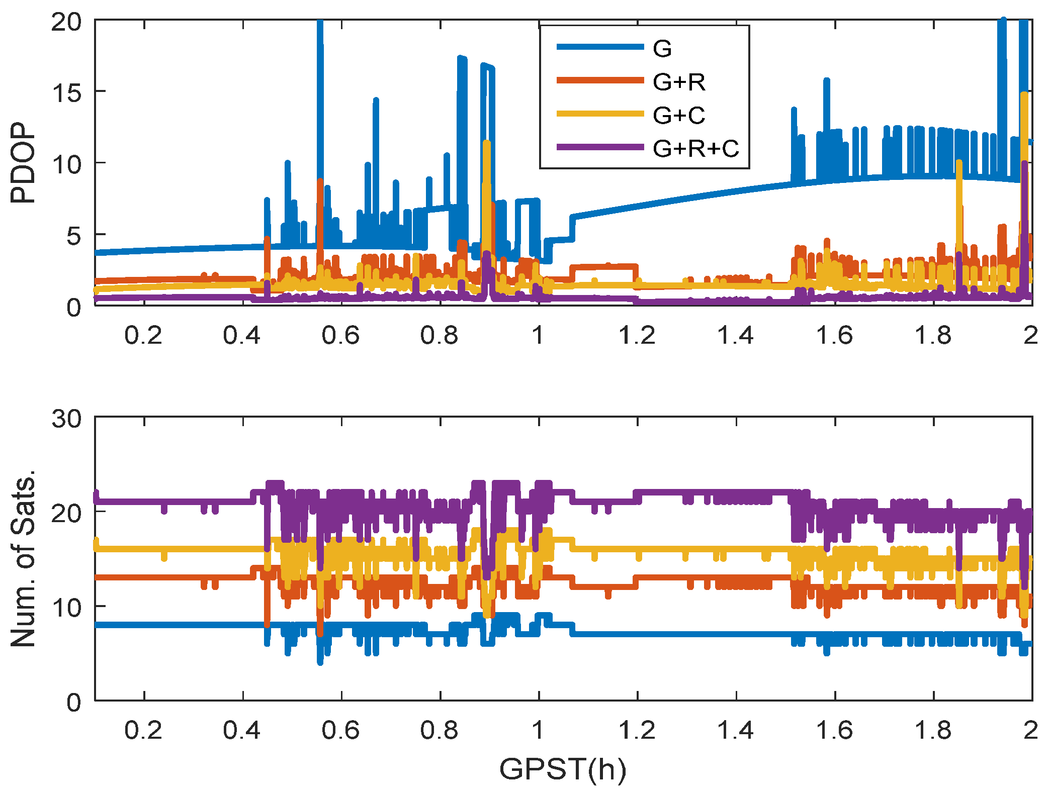
4.2.1. Availability of Multi-Constellation Kinematic PPP

To investigate the benefits of multi-constellation PPP, the availability was analysed in terms of the numbers of visible satellites and the positional dilution of precision (PDOP) value, which is important for quantifying the GNSS positioning accuracy [25].

Figure 2 shows the number of visible satellites and the PDOP values for each processing case. G represents GPS only, G + R represents the GPS/GLONASS combination, G + C represents the GPS/BDS combination, and G + R + C represents the GPS/GLONASS/BDS combination (as mentioned below). As shown in this figure, the GPS-only geometry was weaker than those of the three combined systems. The largest PDOP value of GPS was 20, whereas the PDOP value of the GPS/GLONASS/BDS combination was always below 5. The numbers of satellites and the PDOP values of the four systems varied very stably in the first 0.4 h and from 1.1 to 1.5 h. In contrast, variation occurred very frequently during the rest of the experimental period. The reason for this result was that the vehicle stayed in static mode for the first 0.4 h and the 1.1–1.5 h. Figure 3 also explains this situation, as it shows the coordinate increments at the directions of north, east and up.

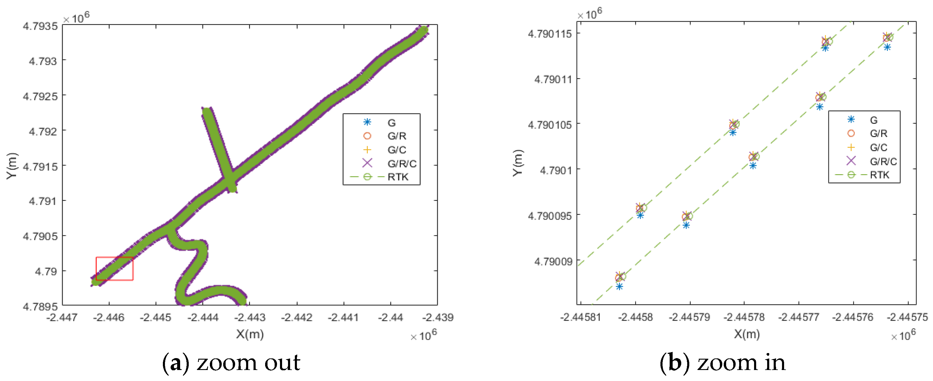
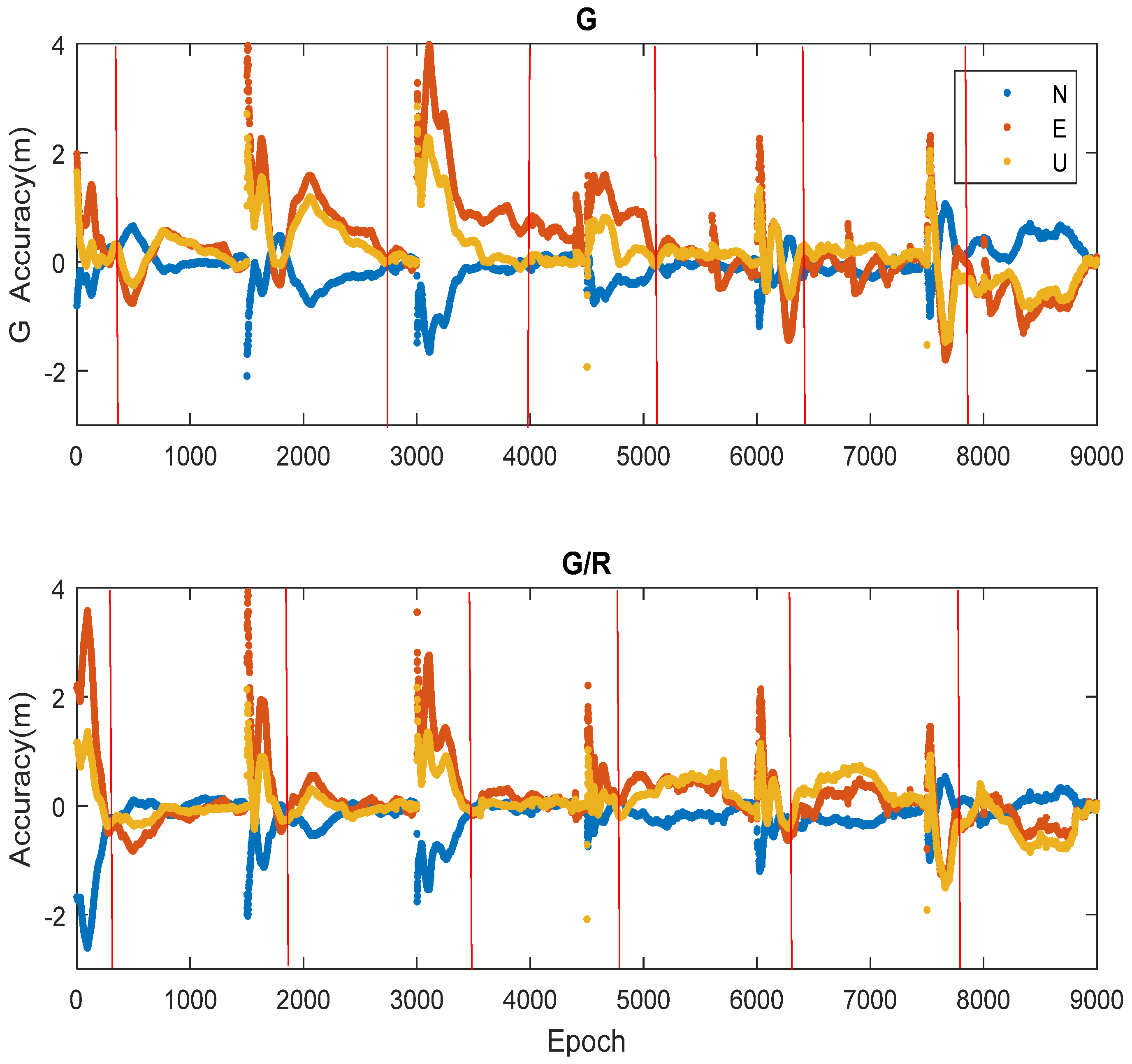
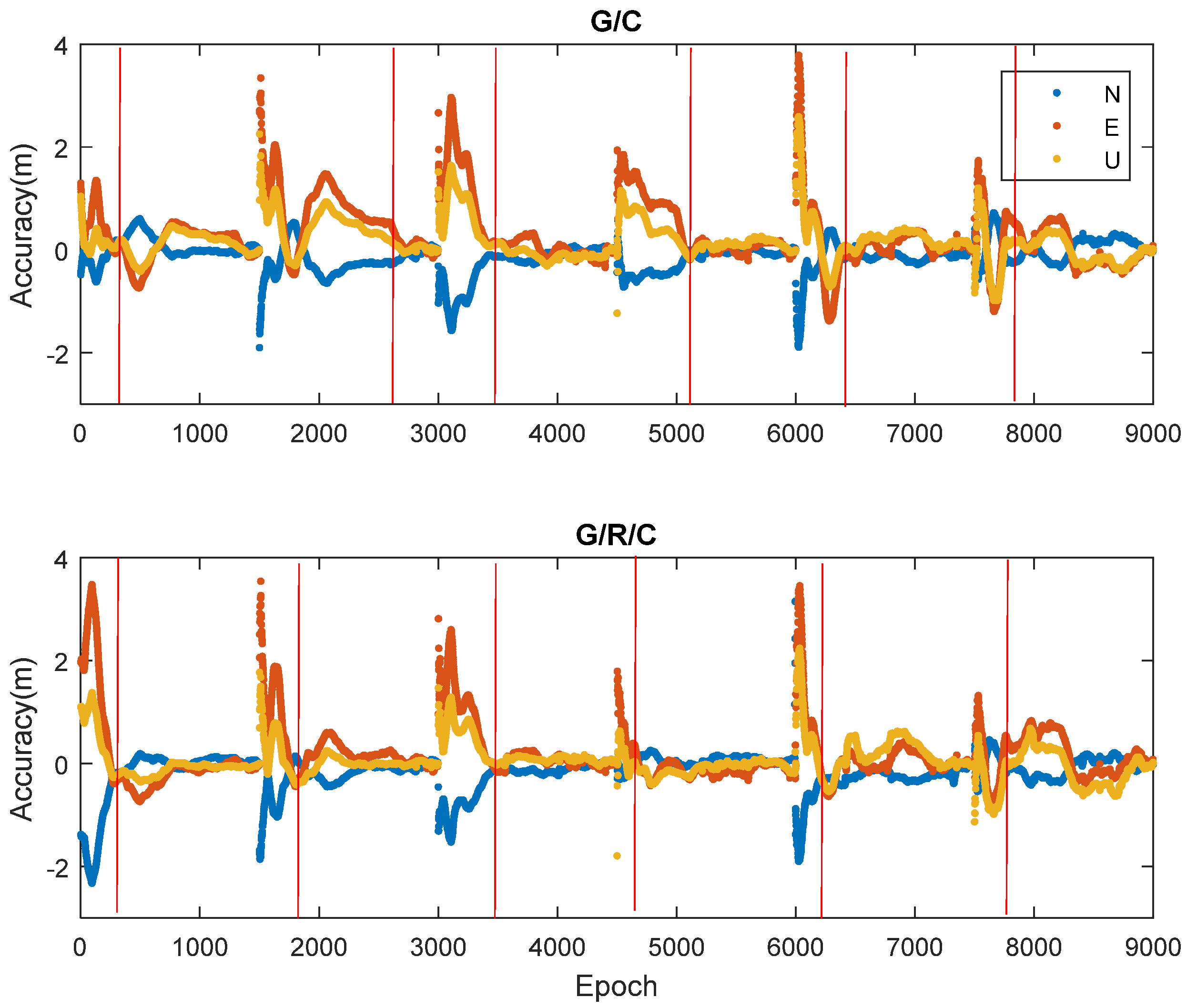
4.2.2. Positioning Accuracy and the RMS of the Kalman Filter

To assess the kinematic positioning accuracy of the multi-constellation PPP, the double difference RTK results were regarded as the true coordinates. These results were computed using the GNSS/INS tightly coupled resolution of Inertial Explorer 8.60 software (IE 8.60), using the multi-constellation signals. The positioning accuracy of this software can reach 1–2 cm. Figure 4a shows the positioning results of multi-constellation kinematic PPP and RTK. When we zoomed in it in Figure 4b, we found that the position of GPS only was very different from that of RTK. There was also little error in the results of the GPS/GLONASS PPP. The positions of the GPS/BDS and GPS/GLONASS/BDS were very similar to those of the RTK. The differences between these RTK coordinates and the PPP results of the GPS only, GPS/GLONASS, GPS/BDS and GPS/GLONASS/BDS were compared to assess the performance of the multi-constellation kinematic PPP in detail. The mean square errors of these differences are shown in

Table 3. The mean errors of the four processing cases (unit: m²). STD: standard deviation.

	STD
	N	E
GPS	0.045	0.085
GPS/GLONASS	0.040	0.080
GPS/BDS	0.013	0.050
GPS/GLONASS/BDS	0.009	0.022

. From Table 3, we can see that the mean square errors of GPS were 0.045 m and 0.085 m in the east and north directions, respectively, which were much larger than those of GPS/BDS. With the GPS/BDS combination, accuracy improved by 71.11% and 41.18% over GPS only in the north and east directions, respectively. However, the positioning accuracy of GPS/GLONASS was slightly poorer than that of the GPS/BDS. The reason would be that there were more visible GPS/BDS satellites than which of GPS/GLAONSS, and the PDOP of GPS/BDS was better than that of GPS/GLAONSS) (Figure 2). The accuracies of GPS/GLONASS/BDS PPP were better than those of GPS/BDS by 30.77% and 56.00%.

The standard deviations (STDs) of these differences are shown in

Table 4. STDs of the positioning errors for the four processing cases (unit: m).

	N	E
GPS	0.067	0.091
GPS/GLONASS	0.062	0.081
GPS/BDS	0.056	0.073
GPS/GLONASS/BDS	0.042	0.060

, and the reference coordinates are the positioning results of the RTK. Smaller STDs indicate better results. As shown in Table 4, the STD of the GPS-only system was relatively large because the number of visible satellites was low (Figure 2). In contrast, the STD of the GPS/GLONASS/BDS PPP was clearly the best.

4.2.3. Convergence Time

To evaluate the convergence performance of multi-constellation kinematic PPP, we started from the data sets in five-minute intervals (i.e., 12 times an hour) until convergence was achieved. In this study, the position filter was considered to be converged when the positioning errors reached ±0.1 m and remained within that range.

Table 5. Mean convergence time of RTK.

	GPS	GPS/BDS	GPS/GLONASS	GPS/GLONASS/BDS
Mean convergence time (min)	64.2	50.9	52.4	47.5

presents the mean convergence time of RTK. Figure 5 and Figure 6 show the kinematic PPP positioning errors of the four different processing cases. In these figures, we only present the convergence performance of PPP based on six replicates because of the space limitations. The convergence time was defined as the period from the first epoch to the converged epoch (indicated as a red line in these figures). Based on these figures and the table, we found that the GPS-only PPP required substantially more time to converge than the other processing cases. In contrast, the convergence performance of the GPS/GLONASS/BDS system was the best for all three coordinate components. Relative to that of GPS-only PPP, the convergence times of GPS/GLONASS and GPS/BDS PPP improved, particularly in the east direction. This result was very similar to that of Cai et al. [22].

5. Conclusions

In this study, the performance of multi-constellation kinematic PPP was assessed in terms of the positioning accuracy and convergence time. A kinematic experimental dataset was processed using a self-developed software based on the multi-constellation kinematic PPP model, Kalman filter and stochastic models. Based on the discussions above, we drew the following conclusions:

• The availability of multi-constellation kinematic PPP was significantly better than that of GPS-only PPP because more satellites were observable and because the PDOP was better.
• The accuracy of multi-constellation kinematic PPP was greater than that of GPS-only, GPS/BDS and GPS/GLONASS PPP. The positioning accuracy of GPS/GLONASS PPP was slightly lower than that of GPS/BDS PPP.
• The convergence performance of GPS/GLONASS/BDS kinematic PPP was the best for all three coordinate components, particularly in the East direction.
• Multi-constellation kinematic PPP can provide a positioning service with centimetre-level accuracy for dynamic users.

References

1. Zumberge, J.F.; Heflin, M.B.; Jefferson, D.C.; Watkins, M.M.; Webb, F.H. Precise point positioning for the efficient and robust analysis of GPS data from large networks. J. Geophys. Res. 1997, 102, 5005–5017. [Google Scholar] [CrossRef]
2. Dow, J.M.; Neilan, R.E.; Rizos, C. The international GNSS service in a changing landscape of global navigation satellite systems. J. Geod. 2009, 83, 191–198. [Google Scholar] [CrossRef]
3. Li, M.; Wickert, M. A novel real-time precise positioning service system: Global precise point positioning with regional augmentation. J. Glob. Position. Syst. 2012, 11, 29. [Google Scholar]
4. Li, X.; Ge, M.; Douša, J.; Wickert, J. Real-time precise point positioning regional augmentation for large GPS reference networks. GPS Solut. 2014, 18, 61–71. [Google Scholar] [CrossRef]
5. Bisnath, S.; Gao, Y. Current state of precise point positioning and future prospects and limitations. In Observing Our Changing Earth; Springer: Berlin, Germany, 2009; pp. 615–623. [Google Scholar]
6. Loyer, S.; Perosanz, F.; Mercier, F.; Capdeville, H.; Marty, J.-C. Zero-difference GPS ambiguity resolution at CNES–CLS IGS analysis Center. J. Geod. 2012, 86, 991–1003. [Google Scholar] [CrossRef]
7. Li, T.; Wang, J.; Laurichesse, D. Modeling and quality control for reliable precise point positioning integer ambiguity resolution with GNSS modernization. GPS Solut. 2014, 18, 429–442. [Google Scholar] [CrossRef]
8. Laurichesse, D.; Mercier, F.; Berthias, J.-P.; Broca, P.; Cerri, L. Integer ambiguity resolution on undifferenced GPS phase measurements and its application to PPP and satellite precise orbit determination. Navigation 2009, 56, 135–149. [Google Scholar] [CrossRef]
9. Ge, M.; Gendt, G.; Rothacher, M.; Shi, C.; Liu, J. Resolution of GPS carrier-phase ambiguities in precise point positioning (PPP) with daily observations. J. Geod. 2008, 82, 389–399. [Google Scholar] [CrossRef]
10. O’Keefe, K. Availability and reliability advantages of GPS/Galileo integration. In Proceedings of the 14th International Technical Meeting of the Satellite Division of the Institute of Navigation (ION GPS-2001), Salt Lake City, UT, USA, 11–14 September 2001.
11. Hewitson, S.; Wang, J. GPS/GLONASS/GALILEO Integration: Separation of Outliers; School of Surveying and Spatial Information Systems, The University of New South Wales: Sydney, Australia, 2003. [Google Scholar]
12. Ji, S.; Chen, W.; Ding, X.; Chen, Y.; Zhao, C.; Hu, C. Potential benefits of GPS/GLONASS/GALILEO integration in an urban canyon–Hong Kong. J. Navig. 2010, 63, 681–693. [Google Scholar] [CrossRef]
13. Li, X.; Ge, M.; Dai, X.; Ren, X.; Fritsche, M.; Wickert, J.; Schuh, H. Accuracy and reliability of multi-GNSS real-time precise positioning: GPS, GLONASS, BeiDou, and Galileo. J. Geod. 2015, 89, 607–635. [Google Scholar] [CrossRef]
14. Li, X.; Zhang, X.; Ren, X.; Fritsche, M.; Wickert, J.; Schuh, H. Precise positioning with current multi-constellation global navigation satellite systems: GPS, GLONASS, Galileo and BeiDou. Sci. Rep. 2015, 5. [Google Scholar] [CrossRef] [PubMed]
15. Cai, C.; Gao, Y.; Pan, L.; Dai, W. An analysis on combined GPS/COMPASS data quality and its effect on single point positioning accuracy under different observing conditions. Adv. Space Res. 2013, 54, 818–829. [Google Scholar] [CrossRef]
16. Yigit, C.O.; Gikas, V.; Alcay, S.; Ceylan, A. Performance evaluation of short to long term GPS, GLONASS and GPS/GLONASS post-processed PPP. Surv. Rev. 2014, 46, 155–166. [Google Scholar] [CrossRef]
17. Li, P.; Zhang, X. Integrating GPS and GLONASS to accelerate convergence and initialization times of precise point positioning. GPS Solut. 2014, 18, 461–471. [Google Scholar] [CrossRef]
18. Cai, C.; Gao, Y. Modeling and assessment of combined GPS/GLONASS precise point positioning. GPS Solut. 2013, 17, 223–236. [Google Scholar] [CrossRef]
19. Yang, Y.; Li, J.; Xu, J.; Tang, J.; Guo, H.; He, H. Contribution of the compass satellite navigation system to global PNT users. Chin. Sci. Bull. 2011, 56, 2813–2819. [Google Scholar] [CrossRef]
20. Qu, L.; Zhao, Q.; Li, M.; Guo, J.; Su, X.; Liu, J. Precise point positioning using combined BeiDou and GPS observations. In China Satellite Navigation Conference (CSNC) 2013 Proceedings; Springer: Berlin, Germany, 2013; pp. 241–252. [Google Scholar]
21. Li, M.; Qu, L.; Zhao, Q.; Guo, J.; Su, X.; Li, X. Precise point positioning with the BeiDou navigation satellite system. Sensors 2014, 14, 927–943. [Google Scholar] [CrossRef] [PubMed]
22. Li, W.; Teunissen, P.; Zhang, B.; Verhagen, S. Precise point positioning using GPS and Compass observations. In China Satellite Navigation Conference (CSNC) 2013 Proceedings; Springer: Berlin, Germany, 2013; pp. 367–378. [Google Scholar]
23. Rizos, C.; Montenbruck, O.; Weber, R.; Weber, G.; Neilan, R.; Hugentobler, U. The IGS MGEX experiment as a milestone for a comprehensive multi-GNSS service. In Proceedings of the ION 2013 Pacific PNT Meeting, Honolulu, HI, USA, 23–25 April 2013.
24. Tegedor, J.; Øvstedal, O.; Vigen, E. Precise orbit determination and point positioning using GPS, Glonass, Galileo and BeiDou. J. Geod. Sci. 2014, 4. [Google Scholar] [CrossRef]
25. Cai, C.; Gao, Y.; Pan, L.; Zhu, J. Precise point positioning with quad-constellations: GPS, BeiDou, GLONASS and Galileo. Adv. Space Res. 2015, 56, 133–143. [Google Scholar] [CrossRef]
26. Li, X.; Wang, J.; Liu, C. Heading estimation with real-time compensation based on kalman filter algorithm for an indoor positioning system. ISPRS Int. J. Geo-Inf. 2016, 5. [Google Scholar] [CrossRef]
27. Li, X.; Wang, J.; Liu, C.; Zhang, L.; Li, Z.; Integrated, W. Fi/PDR/Smartphone using an adaptive system noise extended kalman filter algorithm for indoor localization. ISPRS Int. J. Geo-Inf. 2016, 5. [Google Scholar] [CrossRef]
28. Wang, J.; Stewart, M.P.; Tsakiri, M. Stochastic modeling for static GPS baseline data processing. J. Surv. Eng. 1998, 124, 171–181. [Google Scholar] [CrossRef]
29. Gao, C.; Wu, F.; Chen, W.; Wang, W. An improved weight stochastic model in GPS Precise Point positioning. In Proceedings of the 2011 International Conference On Transportation, Mechanical, and Electrical Engineering (TMEE), Changchun, China, 16–18 December 2011.
30. Xu, Y.; Ji, S. Data quality assessment and the positioning performance analysis of BeiDou in Hong Kong. Surv. Rev. 2015, 47, 446–457. [Google Scholar] [CrossRef]
31. Xu, Y.; Ji, S.; Chen, W.; Weng, D. A new ionosphere-free ambiguity resolution method for long-range baseline with GNSS triple-frequency signals. Adv. Space Res. 2015, 56, 1600–1612. [Google Scholar] [CrossRef]
32. Collins, J.P.; Langley, R.B. A Tropospheric Delay Model for the User of the Wide Area Augmentation System; Department of Geodesy and Geomatics Engineering, University of New Brunswick: Fredericton, NB, Canada, 1997. [Google Scholar]
33. Wu, S.C.; Yunck, T.P.; Thornton, C.L. Reduced-dynamic technique for precise orbit determination of low Earth satellites. J. Guid. Contr. Dyn. 1991, 14, 24–30. [Google Scholar] [CrossRef]
34. Kouba, J.; Héroux, P. Precise point positioning using IGS orbit and clock products. GPS Solut. 2001, 5, 12–28. [Google Scholar] [CrossRef]
35. Niell, A.E. Improved atmospheric mapping functions for VLBI and GPS. Earth Planets Space 2000, 52, 699–702. [Google Scholar] [CrossRef]
Figure 1. The vehicle’s route.
Ijgi 06 00006 g001
Figure 2. Numbers of satellites and positional dilution of precision (PDOP) values of multi-constellation PPP. BDS: BeiDou Navigation Satellite System; GLONASS: Globalnaya Navigatsionnaya Sputnikovaya Sistema; GPS: global positioning system; G: GPS only; G + R: GPS/GLONASS combination; G + C: GPS/BDS combination; G + R + C: GPS/GLONASS/BDS combination.
Ijgi 06 00006 g002
Figure 3. Coordinate increments in the following directions: north, east and up.
Ijgi 06 00006 g003
Figure 4. Multi-constellation kinematic PPP and real-time kinematic (RTK) positions.
Ijgi 06 00006 g004
Figure 5. The difference between the PPP kinematic and RTK solutions (GPS and GPS/GLONASS).
Ijgi 06 00006 g005
Figure 6. The difference between the PPP kinematic and RTK solutions (GPS/BDS and GPS/GLONASS/BDS).
Ijgi 06 00006 g006