Road2Vec: Measuring Traffic Interactions in Urban Road System from Massive Travel Routes


1
State Key Laboratory of Resources and Environmental Information System, Institute of Geographic Sciences and Natural Resources Research, CAS, Beijing 100101, China
2
University of Chinese Academy of Sciences, Beijing 100049, China
3
Department of Geography, University of California, Santa Barbara, CA 93106, USA
4
Department of Geography, University of Wisconsin, Madison, WI 53706, USA
5
Fujian Collaborative Innovation Center for Big Data Applications in Governments, Fuzhou 350003, China
6
Jiangsu Center for Collaborative Innovation in Geographical Information Resource Development and Application, Nanjing 210023, China
*
Author to whom correspondence should be addressed.
ISPRS Int. J. Geo-Inf. 2017, 6(11), 321; https://doi.org/10.3390/ijgi6110321
Submission received: 17 August 2017
/
Revised: 6 October 2017
/
Accepted: 24 October 2017
/
Published: 26 October 2017
Abstract
:Good characterization of traffic interactions among urban roads can facilitate traffic-related applications, such as traffic control and short-term forecasting. Most studies measure the traffic interaction between two roads by their topological distance or the correlation between their traffic variables. However, the distance-based methods neglect the spatial heterogeneity of roads’ traffic interactions, while the correlation-based methods cannot capture the non-linear dependency between two roads’ traffic variables. In this paper, we propose a novel approach called Road2Vec to quantify the implicit traffic interactions among roads based on large-scale taxi operating route data using a Word2Vec model from the natural language processing (NLP) field. First, the analogy between transportation elements (i.e., road segment, travel route) and NLP terms (i.e., word, document) is established. Second, the real-valued vectors for road segments are trained from massive travel routes using the Word2Vec model. Third, the traffic interaction between any pair of roads is measured by the cosine similarity of their vectors. A case study on short-term traffic forecasting is conducted with artificial neural network (ANN) and support vector machine (SVM) algorithms to validate the advantages of the presented method. The results show that the forecasting achieves a higher accuracy with the support of the Road2Vec method than with the topological distance and traffic correlation based methods. We argue that the Road2Vec method can be effectively utilized for quantifying complex traffic interactions among roads and capturing underlying heterogeneous and non-linear properties.
1. Introduction
The traffic states of urban roads are often influenced by their neighboring roads. Different terms, such as spatial dependency/relationship in traffic [1,2] and spatial correlation [3,4,5,6], are used in the literature to express such relationship between neighboring roads. In this paper, we use the term traffic interaction to describe the traffic influence between neighboring roads, which is fundamentally caused by the dynamic vehicle movements from one road to another.
Measuring the traffic interactions among urban roads can provide useful information for traffic-related applications. For instance, many studies have reinforced that traffic forecasting accuracy not only depends on forecasting models, but also on the spatio-temporal inputs [4,7,8,9,10,11,12,13]. Identifying the spatio-temporal relationship between neighboring roads has become one of the challenges to traffic forecasting [14].
Existing studies for measuring traffic interactions among urban roads can be categorized as distance-based and correlation-based approaches.
The distance-based approaches assume that road segments within certain topological distances are correlated with each other in traffic [8,9,15,16]. Note that roads within short topological distances are also in direct or indirect upstream-downstream relations. Kamarianakis and Prastacos [7], as well as Min et al. [8], use the topological distance in road network to model the spatial relationship of traffic flow for traffic forecasting. Fusco et al. use the traffic data of each road’s three upstream links and three downstream links as inputs for traffic forecasting [15]. However, such distance-based models neglect the spatial heterogeneity of roads’ traffic interactions. As the traffic flow on a road network is greatly heterogeneous in space, e.g., a minority of roads account for a majority of traffic flow [17,18], the spread of traffic among roads must be anisotropic. For instance, traffic flow on upstream road segments usually do not spread evenly to all downstream road segments, but instead concentrates in certain directions [19]. Therefore, it is necessary to measure the traffic interactions among roads by considering their heterogeneity.
Correlation-based approaches measure the traffic interaction between two roads by calculating the correlation coefficient between their traffic variables, such as volume and speed [1,5]. For instance, Yue and Yeh demonstrate with an empirical example that the cross-correlation function (CCF) can be used to determine the spatial relationship of a road segment with its upstream or downstream neighbors [1]. Such approaches can perform well for freeway systems as each freeway link usually has only one upstream link and one downstream link, hence, the traffic variables between the upstream-downstream links are linearly correlated. However, these approaches are not suitable for the urban road systems, as the correlation coefficient between the two variables is only meaningful for linear relationships. In an urban road system, the traffic variables between two upstream-downstream roads are not exactly linear, as the upstream road may have several downstream roads, and vice versa. Furthermore, the traffic influence not only exists in upstream-downstream roads, but also in the roads that flow into or out of the same road from the same direction [6]. For instance, if road A and road B share a common direct upstream road C, then when road A gets congested, road B may also be influenced as more traffic from road C may flow to road B. If traffic on road A and road B flow into road C, and an increase in traffic on road A contributes to the congestion on road C, then this congestion may propagate backward to road B. Such non-linear traffic interactions cannot be captured correctly by the traditional correlation-based approaches.
Essentially, the traffic influence among roads originates from numerous vehicle movements on road systems; hence, the inherent relationships among roads should be extracted from massive vehicle travel routes. Meanwhile, word embedding techniques, such as Word2Vec model, can probe the underlying relationship between words in the corpus well [20,21,22,23]. As an analogy, in this paper, we propose to quantify the traffic interactions among roads by integrating GPS-enabled vehicle operating travel routes and the Word2Vec model borrowed from the natural language processing (NLP) domain.
More concretely, as each textual document can be represented as sequential words like “word 1, word 2, …, word n”, while each travel route can be represented as sequential road segments like “road segment 1, road segment 2, …, road segment m”, in this paper, each road segment is analogous to a word and each travel route is analogous to a textual document. We use the Word2Vec model to obtain the real-valued vector representation for each road segment (i.e., “word”) from plenty of travel routes (i.e., “textual documents”). According to the principle of word embedding models, a high similarity between two word vectors indicates that the two words co-occur frequently in textual documents (e.g., “boat”-“water”) or their local contexts are very similar (e.g., “boat”-“ship”). Correspondingly, high similarity between two road segment vectors indicates that two road segments frequently co-occur in travel routes or they frequently share common upstream and/or downstream segments in travel routes. Both situations indicate that there are strong traffic interactions.
As a case study, we extract over two million travel routes from floating car data (FCD) collected by GPS-equipped taxies in Beijing, China, and classify them into five datasets according to the departure time of travel routes (i.e., workday morning rush hours, workday evening rush hours, workday non-rush hours, weekends, and holidays). First, we train real-valued vectors for road segments from travel route datasets using the Word2Vec model; then, we measure the traffic interaction between two roads by calculating the similarity of their vectors. Finally, we compare our approach with distance-based and correlation-based approaches by conducting a traffic forecasting process.
The remainder of this paper is structured as follows: Section 2 introduces the principles of the Word2Vec model and presents the workflow for measuring traffic interactions among roads using the proposed Road2Vec model. Section 3 demonstrates this novel approach with a case study, analyzes the findings, and evaluates the results. Section 4 is devoted to discussions. Finally, we provide conclusions and present our vision for future research in Section 5.
2. Materials and Methods
First, we introduce the principles of word embedding techniques and the Word2Vec model; then, we present the workflow for quantifying the traffic interactions among roads using the proposed Road2Vec model.
Note that the Word2Vec is a mathematical model, whereas the proposed Road2Vec is a method/approach for solving a specific problem (i.e., road traffic interactions) by combining the Word2Vec model and large-scale taxi operating route data.
2.1. Word-Embedding Techniques and the Word2Vec Model
2.1.1. Word-Embedding Techniques
Recently, word-embedding techniques have become increasingly popular in NLP. This technique began to develop in 2003 [20], but gained extreme popularity with the Word2Vec model [21] in 2013. The basic idea of word embedding models is to represent each word by a D-dimensional real-valued vector, where D is a relatively small number (typically between 50 and 1000). Such a vector comes to represent, in some abstract way, the semantics of a word, and the distance between two word vectors can be used to measure their semantic similarity (e.g., “boat”-“ship”) and semantic relatedness (e.g., “boat”-“water”). Such vectors are also used as a representational basis for downstream NLP tasks, such as information retrieval, document classification, question answering, named entity recognition, parsing, etc.
There are two main model families for learning word vectors. Count-based methods, such as latent semantic analysis/indexing (LSA/LSI) [22], compute the statistics of how often a word co-occurs with other words in a large text corpus; then, map these count-based statistics down to a small, dense vector for each word using dimension reduction techniques such as singular value decomposition (SVD). Prediction-based methods, such as Word2Vec [21], directly attempt to predict a word from its neighbors in terms of learned small, dense embedding vectors. In fact, the two classes of methods are not dramatically different at a fundamental level, since they both probe the underlying co-occurrence statistics of the corpus [17] and both the semantic similarity and relatedness among words can be captured in practice.
2.1.2. Word2Vec Model
Word2Vec is a predictive model for training word vectors from raw texts. It comes in two formats, the continuous bag-of-words model (CBOW) and the skip-gram model [21]. Algorithmically, the two models are similar, except that CBOW predicts middle (target) words from the surrounding context words, whereas the skip-gram does it the inverse way and predicts surrounding context words from the middle (target) words. CBOW works better if the training data are limited, as it will smooth over the context in each training step. If there is enough training data, a skip-gram model usually performs better.
Next, we briefly introduce the skip-gram model that will be applied to a large-scale dataset in our experiments. Given a sequence of training words , , , …, , the objective of the skip-gram model is to maximize the average log probability:
where is the size of the training window. The inner summation goes from to when computing the log probability of correctly predicting the word given the word in the middle . The outer summation goes over all words in the training corpus.
In the skip-gram model, every word is associated with two learnable parameter vectors, and . They represent the “input” and “output” vectors of the , respectively. The probability of correctly predicting the word , given the word , is calculated by the softmax function:
where is the number of words in the vocabulary.
The Skip-gram and CBOW models are typically trained using a gradient descent based on the back propagation rule [24].
2.2. Measurement of Traffic Interaction among Roads
2.2.1. Analogous Relationships among Routes and Documents
As mentioned above, word-embedding models represent words in a vector space where semantically-similar words are mapped to nearby points. The hypothesis behind these models states that words that appear in the same contexts share semantic meaning. There are two situations for two words that “appear in the same contexts”. The first is that two words frequently co-occur in documents, such as “boat” and “water”, exhibiting semantic relatedness; the second is that the two words’ contextual words in documents are similar, such as “boat” and “ship”, exhibiting semantic similarity.
A textual document is composed of sequential words, whereas a travel route is composed of sequential road segments; regarding each road segment as a word and each travel route as a document, we can obtain the vector representations of road segments by training plenty of travel routes using the word embedding models. We call this method the “Road2Vec”. Correspondingly, high similarity between two road vectors indicates the two roads co-occur frequently in travel routes or they frequently share common upstream or downstream segments along the travel routes. We use two sketch maps of local road systems (Figure 1) to illustrate how both situations exhibit the two road segments closely interact with each other in traffic.
In Figure 1, the line segments connecting small circles represent road segments, and the arrows on them indicate the directions of traffic flow. Road segments with the same color have one common upstream or downstream segments, and their widths of them represent the relative traffic volumes which they source from (their common upstream road segment) or flowing into (their common downstream road segment). Hence, segments 1, 2 and 3 are segment 0’s upstream roads; segments 4, 5 and 6 are segment 0’s downstream roads. The traffic on segment 0 mainly originates from segment 1 and flows to segments 5 and 6.
Two road segments co-occurring frequently along travel routes indicate there are a significant number of vehicles passing through the two roads one after another; therefore, they strongly interact with each other. The downstream traffic state can be influenced by the upstream traffic because of the piling up of vehicles from the upstream road, whereas the downstream traffic state can influence the upstream traffic due to a tailing back of congested vehicles [1]. For instance, if road segment 0 in Figure 2 became congested or blocked due to a traffic accident, road segment 1 would be much more influenced than road segments 2 or 3.
Two road segments frequently sharing common upstream or/and downstream roads in travel routes may interact with each other indirectly through their common upstream or/and downstream roads [6]. For instance, in Figure 1, road segments 5 and 6 share common upstream road segment 0. If segment 5 was blocked due to traffic control or an accident, more traffic from segment 1 may detour to segment 6, which may cause it to become congested. Such traffic interactions through traffic propagations do exist in urban road systems, but are usually neglected in the existing studies.
2.2.2. Training Road Segment Vectors
The vector representation for each road segment is trained using the Word2Vec model. We use a deep learning tool from a Python package called “gensim” (https://radimrehurek.com/gensim/) to train the Word2Vec models in our experiments. The format and parameters of the called function are represented as follows:
model = gensim.models.Word2Vec (documents, dimension = 200, window = 5)
- documents are lists of textual documents, and each document is a list of words in a serial order;
- dimension is the dimension of the word vectors, and reasonable values are in the tens to hundreds; and
- window is the most important parameter that determines how many words will be used as each word’s contexts. For instance, a window equaling to 5 indicates that the five words ahead and five words behind will be used as the contexts for the center word in the training.
2.2.3. Calculating Similarities among Road Segment Vectors
After training the model, we measure the spatial interaction between two roads by calculating the cosine similarity of their word vectors. Higher similarity values indicate stronger traffic interactions.
Given two vectors and , the cosine similarity, cos(θ), is represented using a dot product and magnitude as follows:
where and are components of vector and , respectively.
The resulting similarity ranges from −1, meaning exactly opposite, to 1, meaning exactly the same, with 0 indicating that they are uncorrelated, and in-between values indicating intermediate similarity or dissimilarity.
3. Results
3.1. Data
3.1.1. Road Network
The road network of the city of Beijing, China (Figure 2) is used to conduct the experiments. It contains 26,621 road segments, including expressways, arterial streets, side streets, and collector streets. Each bidirectional road segment is considered to be two different words in the Word2Vec model.
3.1.2. Floating Car Data
Floating car data (FCD) was collected from the GPS-equipped taxis operating in Beijing from 01 January 2011 to 31 May 2011, with a sampling frequency of 50 s. An FCD record consists of the car’s identification, time, coordinates (longitude and latitude), speed, and the occupancy state (loading passengers or not), etc. The FCD are used to generate travel routes which will be used to train Word2Vec models, and to calculate road traffic states that will be used to evaluate the results.
- 1.
- Travel routesWe map all the GPS points between passengers’ pick-up and drop-off locations (i.e., travel trajectories) to the road network using a map matching algorithm called ST-CRF, which can process low-frequency (i.e., sparse) FCD [25]. After mapping each GPS point to a road segment, we proceed as follows:
- (1)
- if more than one consecutive GPS points are mapped onto the same road segment, then the road segment is only counted once in the travel route;
- (2)
- if two consecutive GPS points are mapped onto different road segments that are not topologically adjacent in a road network, then we use the shortest path between the two road segments to form the travel route.
After the processing, we obtain over two million travel routes, which are represented by sequential road segments. A route is represented as follows:
where is the number of road segments included on route . Considering the temporal heterogeneity of road traffic interactions, we divide these routes into five datasets according to the departure time of the routes: workday morning rush hours (7:00–9:00), workday evening rush hours (17:00–19:00), workday non-rush hours (0:00–7:00; 9:00–17:00; 19:00–24:00), weekends and holidays. Note that there are large numbers of tourists in Beijing on holidays, during which the traffic volumes on the road network are enormous.
- 2.
- Traffic statesThe speed on each road segment in each time interval on each day is extracted from the FCD by calculating the average speeds of the passing cars during the current time interval. If there is no car passing through during the current time interval, then, we use a valid value from another day in the same time interval as an alternative. Because we set the period of each time interval as 5 min, there are 288 total time intervals in a day. For each road segment, the speed data on different days are reconstructed into five long time series according to the period, that is, workday morning rush hours, workday evening rush hours, workday non-rush hours, weekends, and holidays. Each of the five long time series is formatted as follows:where represents the total days in the workday/weekend/holiday, while represents the number of intervals in the workday morning rush hours, workday evening rush hours, workday non-rush hours, weekend, or holiday on each corresponding day.
The traffic states will be used to calculate the correlations among roads as a comparative method and make traffic forecasting for evaluation.
3.2. Results
The most important parameter of the Word2Vec models is the window size. In NLP, window sizes are often set at 5, which means the five words ahead and five words behind are used as the center word’s contexts in training. In our case, we trained 40 Word2Vec models with different window sizes ranging from one to eight using the five temporally-divided travel route datasets of workday morning rush hours, workday evening rush hours, workday non-rush hours, weekends, and holidays.
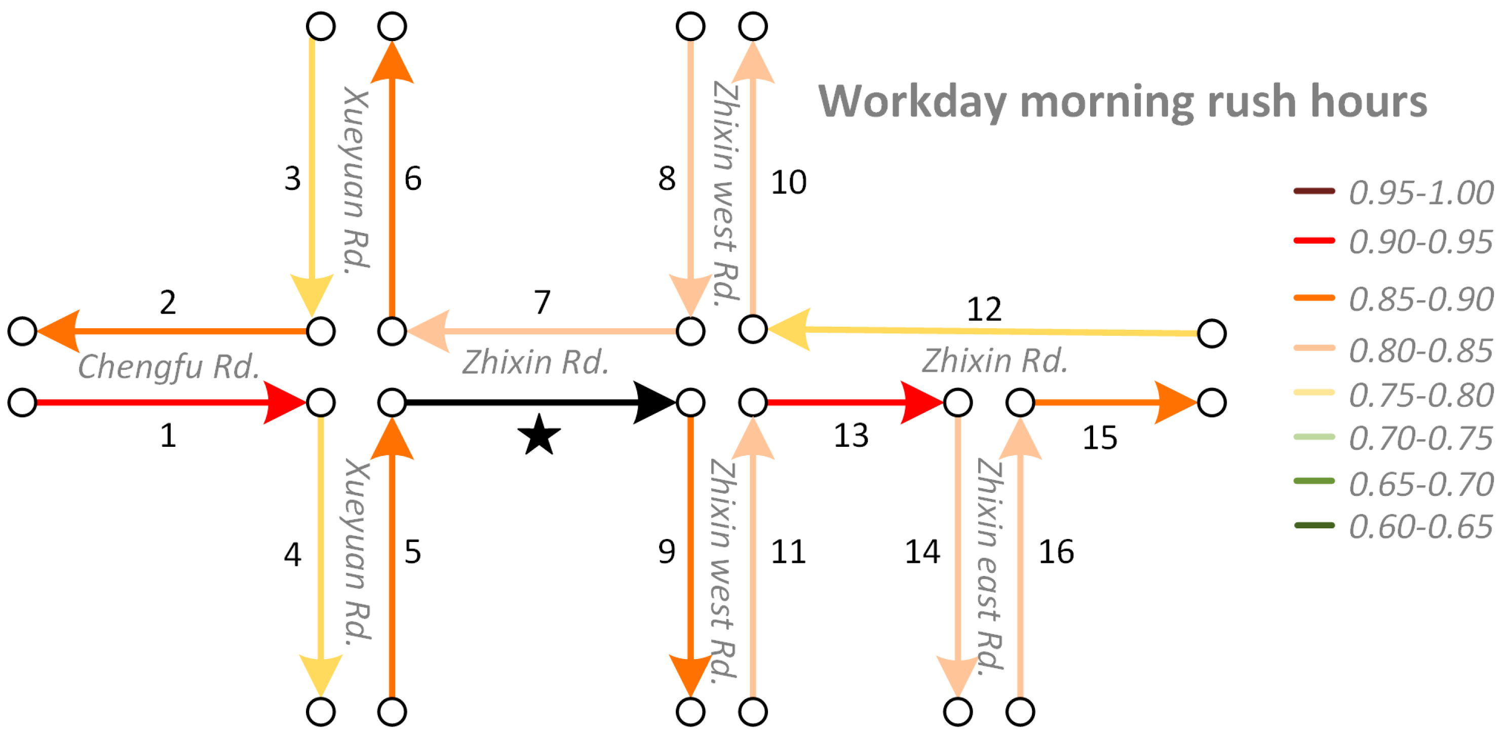
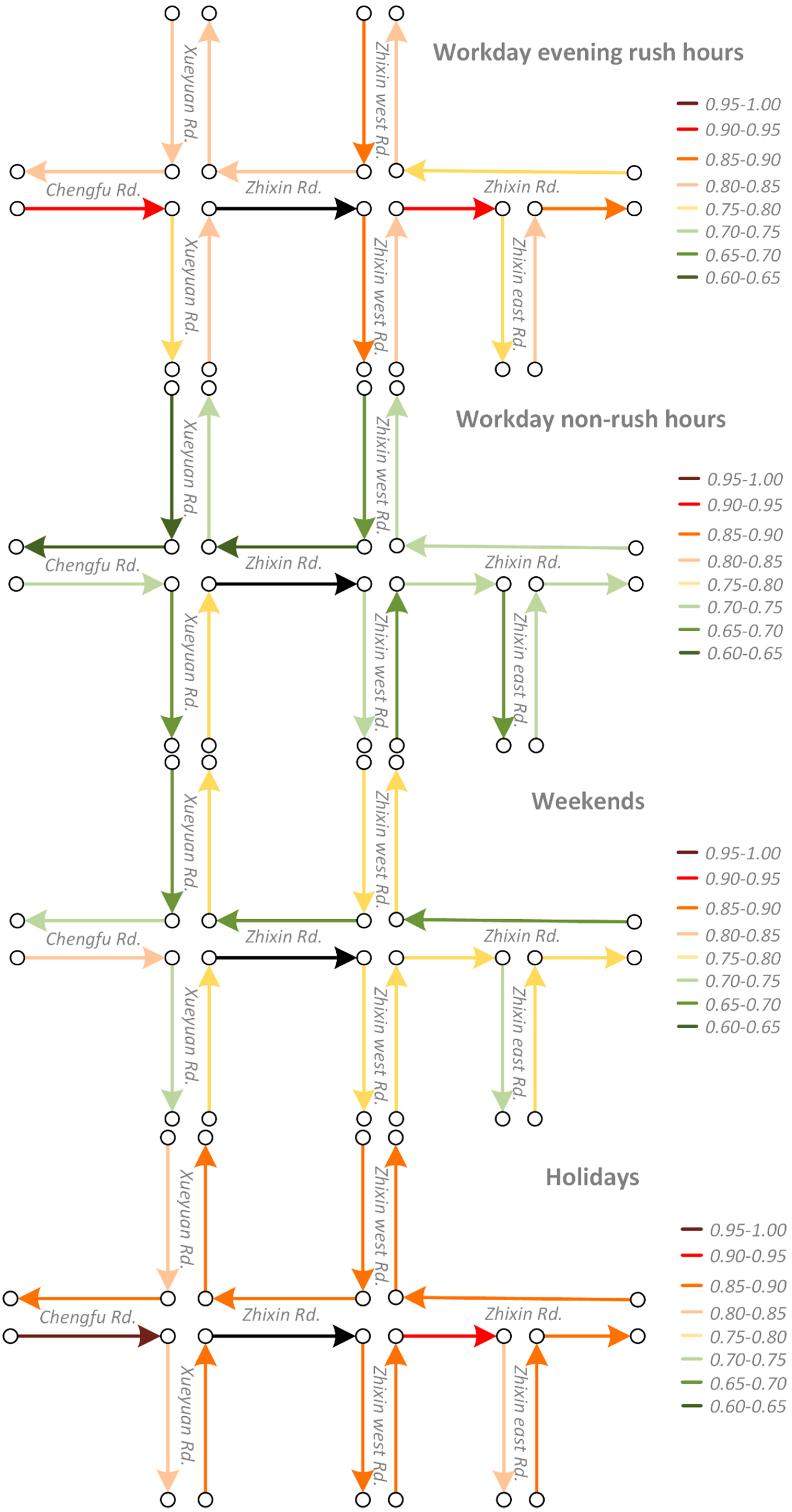
We use a diagrammatic sketch (Figure 3) to demonstrate the cosine similarity between the vectors of “Zhixin Rd.” (the segment labeled with a black star) and its neighbors at different times. Traffic volumes in this area are considerable, as many universities and residential communities are located here. These road segment vectors are trained from Word2Vec models with window sizes equaling to 5. We can find that: (1) the traffic interactions among neighboring roads varies greatly over time. Such interactions are stronger on workday morning rush hours, workday evening rush hours, and holidays compared to workday non-rush hours and weekends. This proves that our approach can capture the temporal heterogeneity of road traffic interactions correctly; and (2) the traffic interactions among neighboring roads are spatially heterogeneous. Taking the results of workday morning rush hours as an example, road segments 9, 10, and 13 are all downstream roads of “Zhixin Rd.”, but the traffic interaction between “Zhixin Rd.” and road segment 13 is stronger than that between “Zhixin Rd” and road segment 10. Furthermore, as we explained in Figure 1, even though some road pairs do not have “upstream-downstream” relationships, such as “Zhixin Rd.” and road segments 6, 8, or 11, but as they share common upstream or downstream road segments, they still interact with each other in traffic.
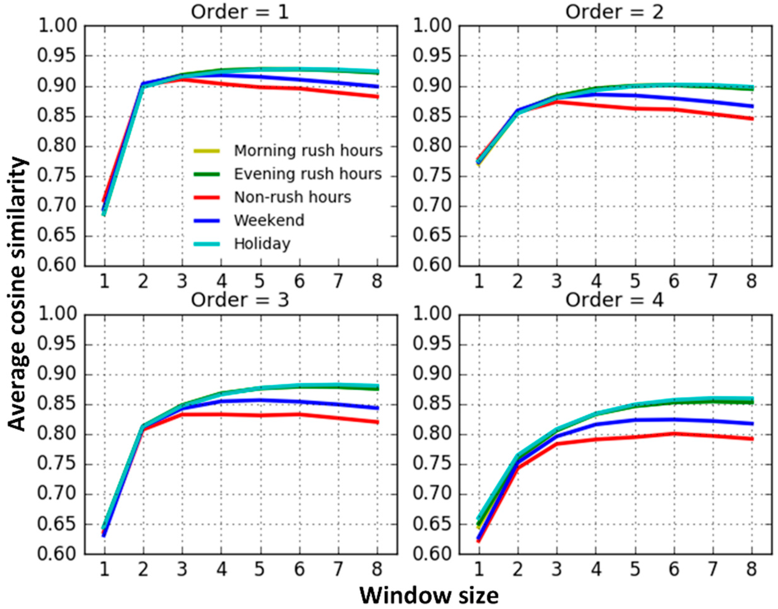
Next, we calculate the average similarities of vectors among the first-order, second-order, third-order, and fourth-order neighboring roads, respectively. The “-order” indicates that the shortest topological distance between two road segments is . From the results shown in Figure 4, we determine the following:
- (1)
- When the window size equals 1, the traffic interactions among roads are very weak and apparently different from the results trained from models with larger window sizes. This may result from the insufficient contextual information attempting to capture road interaction relationships. The results trained from models with the window sizes from two to eight slightly increase at first, and then remain steady.
- (2)
- The average similarity on workday morning rush hours, workday evening rush hours and holidays are relatively similar and they are higher than on weekends and workday non-rush hours. When traffic volumes on the road system are larger, such as during workday peak hours and holidays, road traffic interactions are also stronger. Conversely, when the traffic volumes are relatively small, such as workday non-rush hours and weekends, road interactions are also relatively weaker. The findings match well with the default transportation patterns and this indicates that we correctly capture the temporal heterogeneity of road traffic interaction.
- (3)
- Excluding the results trained from models with window sizes equal to 1, the average similarity between neighboring roads decreases progressively along with an increase in the topological order. That is, on average, topologically-closer road segments have stronger traffic interactions, indicating that our Road2Vec approach also captures the influence of topological distance.
3.3. Results Evaluation
Existing studies indicate that information on the spatial dependency in road traffic is a valuable hint for short-term traffic forecasting [1]. Forecasting accuracy not only depends on forecasting models, but also relates to the spatio-temporal inputs [9,26,27]. Therefore, to prove the effectiveness of our approach, we conduct a five-minute traffic forecasting process and test the performances of the forecasting models with different spatial-temporal inputs selected by topological distance, correlation between speed time series, and our proposed “Road2Vec” method.
Two well-known supervised machine learning models, i.e., artificial neural network (ANN) and support vector machine (SVM), are used for forecasting in this paper, as they are all capable of solving complicated non-linear problems and are frequently used for traffic forecasting [9,14,15,16,28,29].
Given a set of training samples in the form of {(), (), …, ()}, where is the feature vector of the -th sample and is the label, the supervised learning process seeks a function to solve a classification problem, where is the input space and is the output space. Then, given a new sample , one can predict by inputting into the trained model . Most of the machine learning models are non-linear, including ANN and SVM.
In our case, to forecast the speed of road segment on the next time interval (i.e., ), the data inputs contain real-time speeds of the road segment and its traffic-related neighbors during the current time interval . Hence, there are a total of + 1 features as the inputs of the traffic forecasting models. The “most traffic related neighbors” are selected by the topological distance, correlation, and Road2Vec, respectively. In our paper, we choose , because most road segments usually have six first-order neighbors (i.e., the topological distance equals 1) which include three upstream segments and three downstream segments. Note that the most traffic-related neighbors are different in different time periods selected by traffic correlation and Road2Vec, whereas they are fixed in different time periods selected by topological distance.
Instead of using all the road segments to train one model, we train the ANN/SVM model for each road segment (1000 road segments are randomly selected) in the five different time periods (workday morning rush hours, workday evening rush hours, workday non-rush hours, weekends, and holidays) respectively. Therefore, there are a total of 5000 datasets; for each dataset, we use 80% of the samples for training and the rest 20% for testing.
The mean absolute relative error (MARE) is used to evaluate the prediction results:
where is the number of road segments in the experiments; is the number of the time interval used for testing; is the real speed value of road in time interval ; and is the predicted speed value of road in time interval .
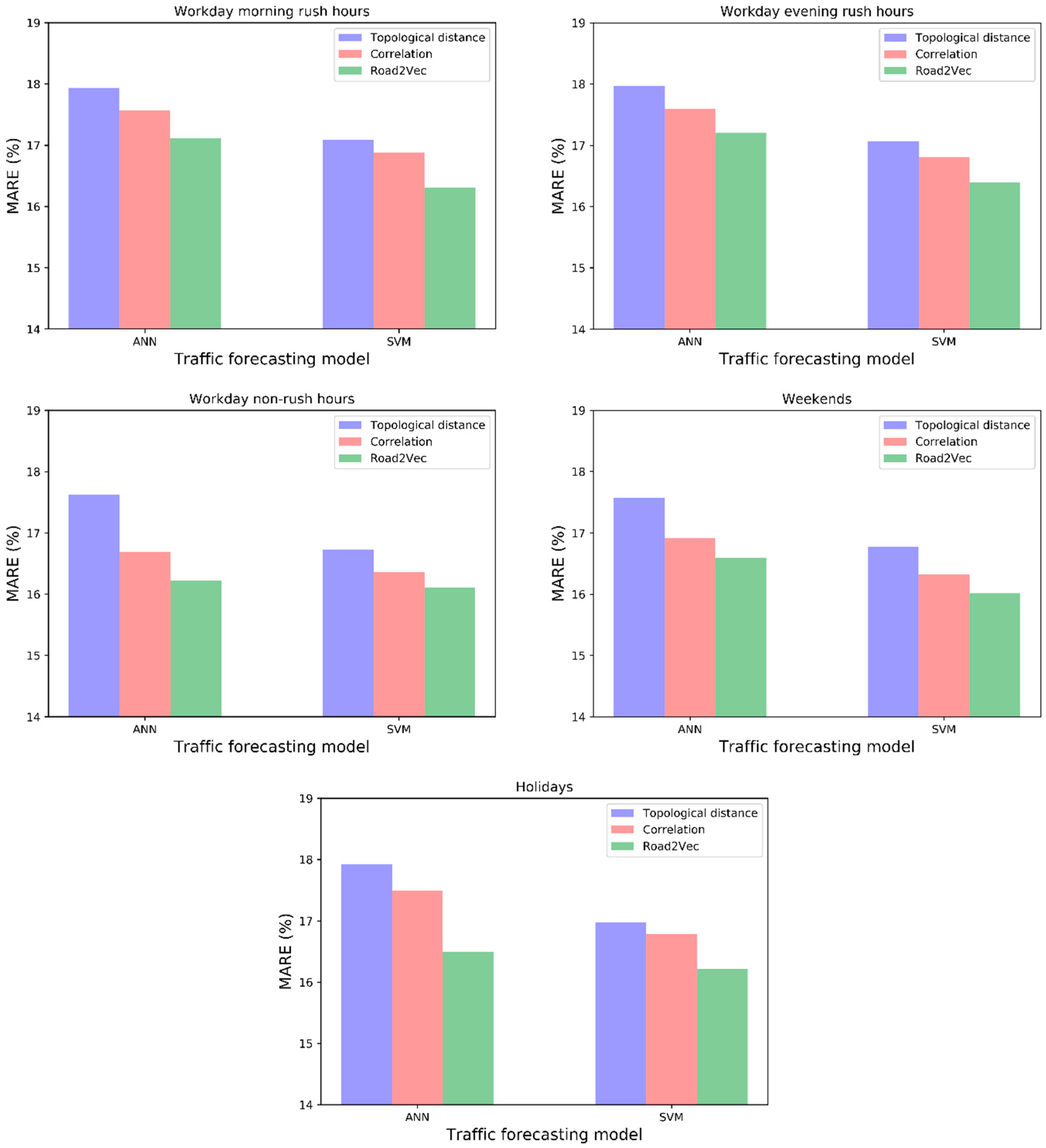
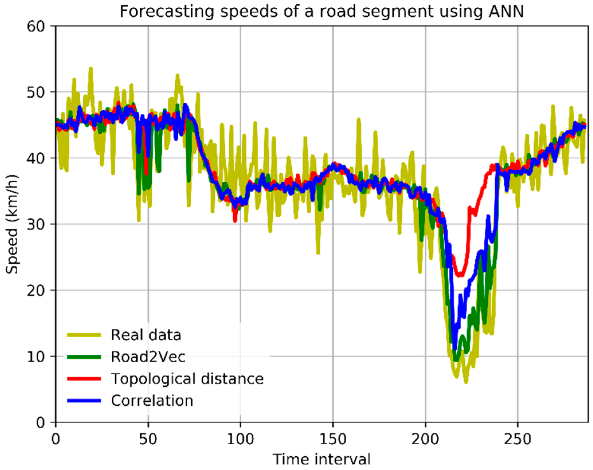
Lower MARE values indicate better prediction power. The forecasting performances in the five different time periods are shown in Figure 5, and the forecasting speeds of a road segment for a whole day are shown in Figure 6.
- (1)
- The forecasting models with spatio-temporal inputs selected by the Road2Vec-based method and the correlation-based method behave better than the topological-distance-based method. This is because the topological-distance-based method neglects the spatio-temporal heterogeneity of traffic influence on urban road systems.
- (2)
- The forecasting models with spatio-temporal inputs selected by the Road2Vec-based method behave better than the correlation-based method during all five periods, which proved that our proposed Road2Vec approach can effectively measure the traffic interactions among urban roads. This is because the Road2Vec can derive the implicit and complicated relationships from the moving trajectories of massive vehicles, whereas a correlation-based method cannot capture the non-linear relationships existing in the urban road system well.
4. Discussion
In this paper, we propose a novel approach to extract the traffic interactions between roads from real travel routes using the NLP word embedding techniques. The key points are summarized as follows:
First, numerous moving vehicles on road networks are “molecules” that form the distributions of traffic flows and create associations among roads. Therefore, measuring the traffic interactions among roads from vehicles’ traces in the real world is a reasonable “cause to effect” and a “bottom-up” process.
Second, the Road2Vec method can measure the traffic interactions not only among upstream-downstream roads, but also among roads that share common upstream or downstream roads. That is, it can capture the implicit and complicated spatial relationships in an urban road system.
As transportation elements (e.g., road segment, travel route) and NLP terms (e.g., word, textual document) have natural analogical relationships, we suggest that other techniques in the text processing domain may also be used in routing behavior and traffic studies in the future.
There are also some limitations in this paper. One may notice that the improvements in the traffic forecasting enhanced by Road2Vec is not that significant compared to the topological-distance and correlation-based methods. This is because that most traffic-related neighbors selected using different methods have an overlap. It is speculated that the Road2Vec method may behave better if applied to the traffic volume data which requires verification in the future work.
It is also worth mentioning that we only use two simplistic models (i.e., ANN and SVM) to test the performances of different traffic interaction measurement methods and do not employ the multiple-layer neural networks (e.g., deep learning models) yet. Existing traffic forecasting methods using deep learning architectures in recent years claim that their approaches can take the spatio-temporal correlations in road systems into account, however, there is no process for establishing spatial relationship in their methods [3], or only roads with linear geometric relationships on straight lines are considered [2]. In subsequent research, we will attempt to integrate the Road2Vec method with a deep learning architecture to further improve traffic forecasting performance.
5. Conclusions
Gaining insight into the spatio-temporal relationships among urban roads in transportation is essential to improving the performance of traffic-related applications. The spatial interactions among roads originate from dynamic movements of massive vehicles. In this research, we propose to investigate the spatio-temporal relationships among roads from the massive vehicular trajectories in the urban road system. Large-scale GPS-enabled taxi routes and NLP word-embedding models are integrated to represent the underlying complex interactions among road segments. With a short-term traffic forecasting experiment, we conclude that the proposed Road2Vec approach outperforms the distance-based and correlation-based approaches in measuring the traffic interactions in the urban road system. The Road2Vec approach can capture the traffic interactions among roads because it has the capability to identify the implicit relationships among roads from the vehicle movements. We will subsequently integrate the Road2Vec approach with more advanced models to further improve the performance of traffic-related applications.
Acknowledgments
This research was supported by the National Natural Science Foundation of China (grant No. 41631177), Key Project of the Chinese Academy of Sciences, ZDRW-ZS-2016-6-3, the National Key Research and Development Program (grant no. 2016YFB0502104), the University of Wisconsin–Madison, Office of the Vice Chancellor for Research and Graduate Education with funding from the Wisconsin Alumni Research Foundation and the UCAS Joint PhD Training Program. Their support is gratefully acknowledged. We also thank the anonymous referees for their helpful comments and suggestions.
Author Contributions
Kang Liu and Song Gao conceived and designed the experiments; Kang Liu and Peiyuan Qiu performed the experiments; Xiliang Liu and Bo Yan explained the details of the model that is used in this paper; and Kang Liu and Feng Lu wrote the paper.
Conflicts of Interest
The authors declare no conflict of interest.
References
- Yue, Y.; Yeh, A.G.O. Spatiotemporal Traffic-Flow Dependency and Short-Term Traffic Forecasting. Environ. Plan. B Plan. Des. 2008, 35, 762–771. [Google Scholar] [CrossRef]
- Ma, X.; Dai, Z.; He, Z.; Ma, J.; Wang, Y.; Wang, Y. Learning Traffic as Images: A Deep Convolutional Neural Network for Large-Scale Transportation Network Speed Prediction. Sensors 2017, 17, 818. [Google Scholar] [CrossRef] [PubMed]
- Lv, Y.; Duan, Y.; Kang, W.; Li, Z.; Wang, F.Y. Traffic Flow Prediction with Big Data: A Deep Learning Approach. IEEE Trans. Intell. Transp. Syst. 2015, 16, 865–873. [Google Scholar] [CrossRef]
- Yang, S.; Shi, S.; Hu, X.; Wang, M. Spatiotemporal Context Awareness for Urban Traffic Modeling and Prediction: Sparse Representation Based Variable Selection. PLoS ONE 2015, 10, e0141223. [Google Scholar] [CrossRef] [PubMed]
- Cai, P.; Wang, Y.; Lu, G.; Chen, P.; Ding, C.; Sun, J. A spatiotemporal correlative k-nearest neighbor model for short-term traffic multistep forecasting. Transp. Res. Part. C Emerg. Technol. 2016, 62, 21–34. [Google Scholar] [CrossRef]
- Cheng, T.; Haworth, J.; Wang, J. Spatio-temporal autocorrelation of road network data. J. Geogr. Syst. 2012, 14, 389–413. [Google Scholar] [CrossRef]
- Kamarianakis, Y.; Prastacos, P. Space-time modeling of traffic flow. Comput. Geosci. 2005, 31, 119–133. [Google Scholar] [CrossRef]
- Min, X.; Hu, J.; Zhang, Z. Urban traffic network modeling and short-term traffic flow forecasting based on GSTARIMA model. In Proceedings of the 13th International IEEE Conference on Intelligent Transportation Systems, Funchal, Portugal, 19–22 September 2010; pp. 1535–1540. [Google Scholar]
- Ishak, S.; Kotha, P.; Alecsandru, C. Optimization of Dynamic Neural Network Performance for Short-Term Traffic Prediction. Transp. Res. Record: J. Transp. Res. Board 2003, 1836, 45–56. [Google Scholar] [CrossRef]
- Min, W.; Wynter, L. Real-time road traffic prediction with spatio-temporal correlations. Transp. Res. Part. C Emerg. Technol. 2011, 19, 606–616. [Google Scholar] [CrossRef]
- Ding, Q.Y.; Wang, X.F.; Zhang, X.Y.; Sun, Z.Q. Forecasting Traffic Volume with Space-Time ARIMA Model. Adv. Mater. Res. 2011, 156–157, 979–983. [Google Scholar] [CrossRef]
- Chan, K.Y.; Khadem, S.; Dillon, T.S.; Palade, V.; Singh, J.; Chang, E. Selection of Significant On-Road Sensor Data for Short-Term Traffic Flow Forecasting Using the Taguchi Method. IEEE Trans. Ind. Inform. 2012, 8, 255–266. [Google Scholar] [CrossRef]
- Yang, S. On feature selection for traffic congestion prediction. Transp. Res. Part. C Emerg. Technol. 2013, 26, 160–169. [Google Scholar] [CrossRef]
- Vlahogianni, E.I.; Karlaftis, M.G.; Golias, J.C. Short-term traffic forecasting: Where we are and where we’re going. Transp. Res. Part C: Emerg. Technol. 2014, 43, 3–19. [Google Scholar] [CrossRef]
- Fusco, G.; Colombaroni, C.; Comelli, L.; Isaenko, N. Short-term traffic predictions on large urban traffic networks: Applications of network-based machine learning models and dynamic traffic assignment models. In Proceedings of the 2015 International Conference on Models and Technologies for Intelligent Transportation Systems (MT-ITS), Budapest, Hungary, 3–5 June 2015; pp. 93–101. [Google Scholar]
- Csikós, A.; Viharos, Z.J.; Kis, K.B.; Tettamanti, T.; Varga, I. Traffic speed prediction method for urban networks-an ANN approach. In Proceedings of the 2015 International Conference on Models and Technologies for Intelligent Transportation Systems (MT-ITS), Budapest, Hungary, 3–5 June 2015; pp. 102–108. [Google Scholar]
- Jiang, B. Street hierarchies: a minority of streets account for a majority of traffic flow. Int. J. Geogr. Inf. Sci. 2009, 23, 1033–1048. [Google Scholar] [CrossRef]
- Gao, S.; Wang, Y.; Gao, Y.; Liu, Y. Understanding Urban Traffic-Flow Characteristics: A Rethinking of Betweenness Centrality. Environ. Plan. B-Plan. Des. 2013, 40, 135–153. [Google Scholar] [CrossRef]
- Liu, X.; Lu, F.; Zhang, H.; Qiu, P. Intersection delay estimation from floating car data via principal curves: A case study on Beijing’s road network. Front. Earth Sci. 2013, 7, 206–216. [Google Scholar] [CrossRef]
- Bengio, Y.; Ducharme, R.; Vincent, P.; Jauvin, C. A Neural Probabilistic Language Model. J. Mach. Learn. Res. 2003, 3, 1137–1155. [Google Scholar]
- Mikolov, T.; Chen, K.; Corrado, G.; Dean, J. Efficient Estimation of Word Representations in Vector Space. In Proceedings of the Workshop at International Conference on Learning Representations, Scottsdale, AZ, USA, 2–4 May 2013; pp. 1–12. [Google Scholar]
- Deerwester, S.; Dumais, S.T.; Furnas, G.W.; Landauer, T.K.; Harshman, R. Indexing by Latent Semantic Analysis. J. Am. Soc. Inf. Sci. 1990, 41, 391–407. [Google Scholar] [CrossRef]
- Pennington, J.; Socher, R.; Manning, C.D. Glove: Global vectors for word representation. In Proceedings of the Conference on Empirical Methods in Natural Language Processing, Doha, Qatar, 25–29 October 2014; pp. 1532–1543. [Google Scholar]
- Rumelhart, D.; Hinton, G.; Williams, R. Learning representations by back-propagating errors. Nature 1986, 323, 533–536. [Google Scholar] [CrossRef]
- Liu, X.; Liu, K.; Li, M.; Lu, F. A ST-CRF Map-Matching Method for Low-Frequency Floating Car Data. IEEE Trans. Intell. Transp. Syst. 2017, 18, 1241–1254. [Google Scholar] [CrossRef]
- Petty, K.F.; Bickel, P.; Ostland, M.; Rice, J.; Schoenberg, F.; Jiang, J.; Ritov, Y. Accurate estimation of travel times from single-loop detectors. Transp. Res. Part A Policy Pract. 1998, 32, 1–17. [Google Scholar] [CrossRef]
- Vythoulkas, P. Alternative approaches to short term traffic forecasting for use in driver information systems. Transp. Traffic Theory 1993, 12, 485–506. [Google Scholar]
- Basu, D.; Maitra, B. Modeling stream speed in heterogeneous traffic environment using ANN-lessons learnt. Transport 2006, 21, 269–273. [Google Scholar]
- Vanajakshi, L.; Rilett, L.R. A comparison of the performance of artificial neural networks and support vector machines for the prediction of traffic speed. In Proceedings of the IEEE Intelligent Vehicles Symposium, Parma, Italy, 14–17 June 2004; pp. 194–199. [Google Scholar]
Figure 1.
Sketch maps of traffic interactions among roads.
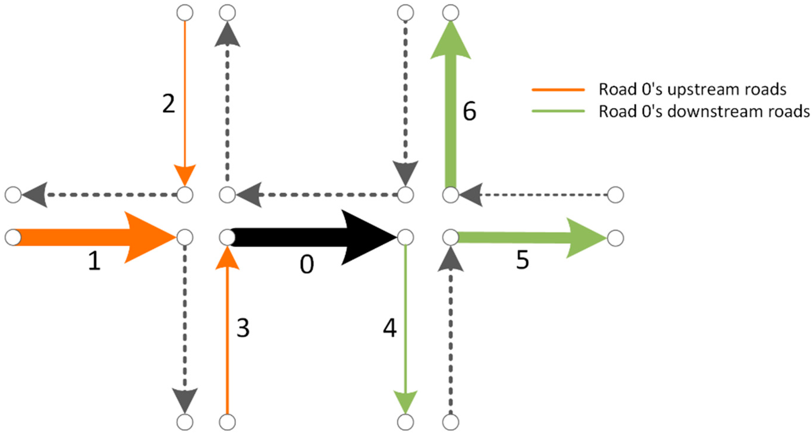
Figure 2.
Road network of the city of Beijing.
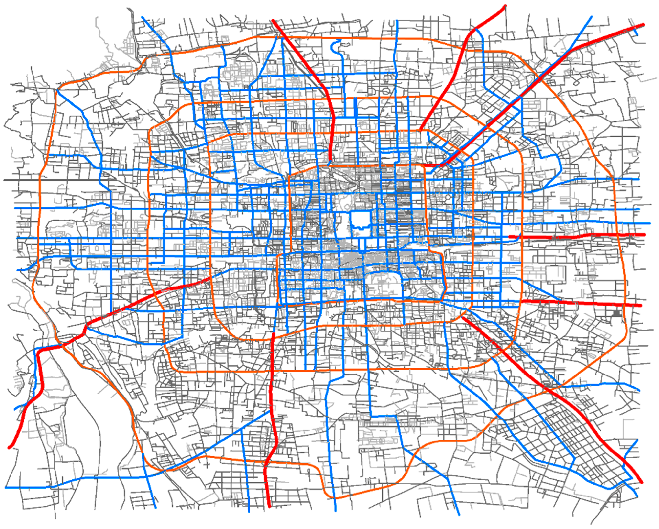
Figure 3.
Traffic interactions between a road segment and its neighbors.


Figure 4.
Average cosine similarities between -order neighboring road segments’ vectors.

Figure 5.
The performance of traffic forecasting models enhanced by different traffic interaction measurement methods.
Figure 5.
The performance of traffic forecasting models enhanced by different traffic interaction measurement methods.

Figure 6.
Forecasting vehicular speeds of a road segment using ANN with different spatio-temporal inputs.
Figure 6.
Forecasting vehicular speeds of a road segment using ANN with different spatio-temporal inputs.
© 2017 by the authors. Licensee MDPI, Basel, Switzerland. This article is an open access article distributed under the terms and conditions of the Creative Commons Attribution (CC BY) license (http://creativecommons.org/licenses/by/4.0/).
Share and Cite
MDPI and ACS Style
Liu, K.; Gao, S.; Qiu, P.; Liu, X.; Yan, B.; Lu, F. Road2Vec: Measuring Traffic Interactions in Urban Road System from Massive Travel Routes. ISPRS Int. J. Geo-Inf. 2017, 6, 321. https://doi.org/10.3390/ijgi6110321
AMA Style
Liu K, Gao S, Qiu P, Liu X, Yan B, Lu F. Road2Vec: Measuring Traffic Interactions in Urban Road System from Massive Travel Routes. ISPRS International Journal of Geo-Information. 2017; 6(11):321. https://doi.org/10.3390/ijgi6110321
Chicago/Turabian StyleLiu, Kang, Song Gao, Peiyuan Qiu, Xiliang Liu, Bo Yan, and Feng Lu. 2017. "Road2Vec: Measuring Traffic Interactions in Urban Road System from Massive Travel Routes" ISPRS International Journal of Geo-Information 6, no. 11: 321. https://doi.org/10.3390/ijgi6110321
Note that from the first issue of 2016, this journal uses article numbers instead of page numbers. See further details here.