The SSP-Tree: A Method for Distributed Processing of Range Monitoring Queries in Road Networks


College of Information and Communication Engineering, Sungkyunkwan University, Suwon 440-746, Korea
*
Author to whom correspondence should be addressed.
ISPRS Int. J. Geo-Inf. 2017, 6(11), 322; https://doi.org/10.3390/ijgi6110322
Submission received: 11 August 2017
/
Revised: 12 October 2017
/
Accepted: 24 October 2017
/
Published: 26 October 2017
(This article belongs to the Special Issue Discovery and Prediction of Moving Objects in Databases using GIS-based Tools)
Abstract
:This paper addresses the problem of processing range monitoring queries, each of which continuously retrieves moving objects that are currently located within a given query range. In particular, this paper focuses on processing range monitoring queries in the road network, where movements of the objects are constrained by a predefined set of paths. One of the most important challenges of processing range monitoring queries is how to minimize the wireless communication cost and the server computation cost, both of which are heavily dependent on the amount of location-update stream generated by moving objects. The traditional centralized methods for range monitoring queries assume that moving objects periodically send location-updates to the server. However, when the number of moving objects becomes increasingly large, such an assumption may no longer be acceptable because the amount of location-update stream becomes enormous. Recently, some distributed methods have been proposed, where moving objects utilize their available computational capabilities for sending location-updates to the server only when necessary. Unfortunately, the existing distributed methods only deal with the objects moving in Euclidean space, and thus they cannot be extended to processing range monitoring queries over the objects moving along the road network. In this paper, we propose the distributed method for processing range monitoring queries in the road network. To utilize the computational capabilities of moving objects, we introduce the concept of vicinity region. A vicinity region, assigned to each moving object o, makes o monitor whether or not it should be included in the results of nearby queries. The proposed method includes (i) a new spatial index structure, called the Segment-based Space Partitioning tree (SSP-tree) whose role is to efficiently search the appropriate vicinity regions for moving objects based on their heterogeneous computational capabilities and (ii) the details of the communication strategy between the server and moving objects, which significantly reduce the wireless communication cost as well as the server computation cost. Through simulations, we verify the effectiveness for processing range monitoring queries over a large number of moving objects (up to 100,000) in the road network (modeled as an undirected graph).
1. Introduction
The proliferation of handheld computing devices equipped with positioning systems has led to the rapid growth of Location-Based Services (LBSs) [1]. In this paper, we study the problem of processing range monitoring queries. A range monitoring query , issued over a set of moving objects O, (i) retrieves a subset of moving objects (⊆O) that are located within a query distance from a query point ; and (ii) continuously updates as the moving objects change their location. Range monitoring queries often play an important role for supporting LBSs. For example, let us consider the following scenarios. A gas station owner (i.e., client) wants to send promotional coupons to all cars (i.e., moving objects) currently located near her gas station; a child safety service provider (i.e., client) wants to monitor the potential dangerous areas to alert parents when their children (i.e., moving objects) enter these areas; a traffic management department wants to monitor the traffic conditions of the main highways in a city. In such scenarios, the functionality of monitoring moving objects that are currently located within a region of interest is highly required.
A large number of methods for processing range monitoring queries were proposed [2,3,4,5,6,7,8,9,10,11,12,13,14], which can be broadly classified into two categories according to the mobility of query points; one deals with static query points (e.g., facilities such as the gas station mentioned above) [2,3,4,5,6,7], whereas the other deals with moving query points (e.g., free taxis looking for the nearby passengers) [8,9,10,11,12,13,14]. Our proposed method belongs to the former category. Most existing methods for processing range monitoring queries are highly centralized in the sense that moving objects periodically send location-updates to the server, and that the server carries out all the computations for processing range monitoring queries [1]. Therefore, their focus is developing algorithms for efficiently process the queries at the server side. However, when the number of moving objects becomes very large, they may suffer from a severe communication bottleneck as well as overwhelming server workload due to a huge amount of location-update stream generated by the moving objects.
One of the key challenges of processing range monitoring queries is how to minimize the wireless communication cost and the server computation cost, both of which heavily depend on the amount of location-update stream. As the amount of location-update stream is increased, the wireless communication cost and the server computation cost are also increased accordingly. Recently, some distributed methods, which aim to reduce the amount of location-update stream by utilizing the computational capabilities of moving objects, have been proposed [2,3]. In the distributed methods, the server assigns each moving object o several queries, and o locally monitors its movement against these queries. Only when o affects the current result of any of the assigned queries, does it send a location-update to the server to let the server update the result of the corresponding query. As such, in the distributed methods, moving objects no longer need to periodically send location-updates to the server, and thus the amount of location-update stream can be reduced. The additional benefit of the distributed methods is that the moving objects can save energy consumption by reducing the number of wireless message transmissions (i.e., the number of location-updates sent to the server). Please note that a wireless message transmission is an energy expensive operation.
Unfortunately, the existing distributed methods only deal with the objects moving freely in Euclidean space. In most real-life scenarios of LBSs, the objects are allowed to move only on a pre-defined set of paths specified by the underlying road network. In Euclidean space, the distance between a moving object o and a query point is defined as the length of the straight-line connecting them, whereas in the road network, the distance between o and is defined as the total length of the shortest path connecting them. Therefore, the existing distributed methods cannot support range monitoring queries in the road network. For example, let us consider a range monitoring query , where is shown in Figure 1 and . As shown in Figure 1a, if q is issued over a set of moving object in Euclidean space, its current result is , where the red circle in the figure represents the query range of q. On the other hand, as shown in Figure 1b, if q is issued over O in the road network, its current result is , where a set of red line segments in the figure represents the query range of q. (Note: Each number in brackets in Figure 1b indicates the distance between and in the road network.) We refer to each line segment that belongs to the query range in the road network as the query segment.
In this paper, we propose the distributed method for processing range monitoring queries in the road network. To utilize the computational capabilities of moving objects, we introduce the concept of vicinity region. Given a moving object o, o’s vicinity region, denoted by , is a rectangular region, which contains (i) the point of o’s current location and (ii) a number of query segments. By letting the server assign o (i) and (ii) query segments inside , o can monitor by itself whether it affects the results of nearby queries while it is moving. The moving object o sends a location-update to the server whenever (i) it leaves or (ii) it affects the result of some nearby query q. In the former case, the server assigns o a new vicinity region together with new query segments, while in the latter case, the server updates the result of q accordingly.
One critical problem is how to determine the suitable size of a vicinity region for each moving object o. If is too small, o needs to frequently send a location-update to the server for receiving a new vicinity region. On the other hand, if is too large, o needs to monitor a large number of queries, which imposes a computationally intensive burden on o. In general, a handheld computing device carried by o executes multiple applications, and thus if a single LBS application occupies substantial computational resources, the service quality of the other applications may deteriorate drastically. With this problem in mind, we propose a new spatial index structure, called the Segment-based Space Partitioning tree (SSP-tree). The role of the SSP-tree to efficiently search the appropriate vicinity regions for moving objects based on their heterogeneous computational capabilities. We also describe the details of the communication strategy between the server and moving objects for cooperative processing of range monitoring queries in the road network.
In summary, we propose (i) the concept of vicinity region; (ii) the SSP-tree for vicinity region search; and (iii) the vicinity region based communication strategy between the server and moving objects for distributed processing of static range monitoring queries. Through simulations, we verify the effectiveness of the proposed method for processing static range monitoring queries in terms of the wireless communication cost and the server computation cost.
2. Problem Statement and System Overview
2.1. Background and Problem Statement
In this paper, we address the problem of processing range monitoring queries in the road network. The road network is modeled as an undirected graph , where is a set of vertices and is a set of edges. A vertex corresponds to a road intersection or dead-end. On the other hand, an edge ∈ E corresponds to a road segment, which connects two vertices and . For convenience of notation, we sometimes indicate an edge as e. We can assume that each road segment of the road network is a straight line because a curved road segment can be transformed into a set of straight lines by adding extra vertices and edges to G. Therefore, the length of an edge can be the Euclidean distance between its two endpoints and . Hereafter, we use to denote the Euclidean distance between any two points (including the vertices) in the road network G.
Definition 1.
Given two vertices and in the road network , where , a path from to , denoted by , is a sequence of vertices such that , , and for each consecutive pair of vertices for all , the condition: holds. Then, the path length of is calculated as:
where and .
Definition 2.
Given two vertices and in the road network , where , there can exist more than one path from to . Then, the shortest path from to , denoted by , is defined as:
where is the set of all the paths from to . The path length of , i.e., , is called the shortest path length.
Consider an example of the road network G in Figure 2a, which serves as a running example in the rest of this paper. In Figure 2a, G consists of 10 vertices and 13 edges. (Note: The vertices and edges outside of the workspace are omitted.) Each number near to each edge in the figure indicates its length (i.e., the Euclidean distance between its two endpoints). From the figure, it can be easily seen that and .
Let O = and Q = be a set of moving objects and a set of range monitoring queries, respectively. Each object is constrained to move only along the edges in the road network G, and thus the point of o’s location, denoted by , at a particular snapshot in time always lies on an edge in G. Each query is represented by a tuple , where is a query point lying on an edge in G and is a query distance.
Definition 3.
Given two points and , where lies on an edge and lies on an edge , the distance between and in the road network G, which is called the network distance (between and ) and denoted by , is defined as:
Given the road network G in Figure 2a, Figure 2b shows the network distance between a query point and several points on G (e.g., vertices and points of moving objects’ location). For example, = and = because , , and lie on the same edge . On the other hand, = + + and = + + . In Figure 2b, each number in brackets indicates the network distance between and each point. (Note: The network distance between and some vertices are omitted for brevity.)
Definition 4.
A range monitoring query , issued over a set of moving objects O, in the road network G, continually retrieves a subset () of moving objects for which the condition: holds.
Definition 5.
Given a query , the query range of q in the road network G, denoted by , is a set of all points on the edges (in G) reachable from within . Formally, and p is a point in .
From Definitions 4 and 5, we can immediately know that given a query and a moving object o () in the road network G, if and only if the point of o’s current location is inside the query range of q, can o be the current result of q (i.e., ⇔ ). In the road network G, the query range of a query q consists of a set of line segments.
Definition 6.
Given an edge in the road network G, a line segment, denoted by , where and are points on , is a set of all points on between and , i.e., the portion of between and .
For example, in Figure 2b, the query range consists of all red line segments (i.e., , , and ), assuming . Please note that, by definition, an edge in is also considered to be a line segment formed by its two endpoints and (i.e., = ). In this paper, we refer to each line segment that belongs to the query range of a query q as the query segment of q, which we denote by or for short. Therefore, given the query range of a query q, each query segment satisfies the condition: ∈ , .
The primary goal of our work is to reduce the amount of location-update stream (generated by moving objects) while maintaining the correct results of range monitoring queries in the road network. To this end, we use the concept of vicinity region so that moving objects send location-updates to the server only when necessary. Given a moving object o, o’s vicinity region is a rectangular region, which contains (i) the point of o’s current location and (ii) some query segments. By assigning each moving object o (i) and (ii) query segments inside , o can locally monitor whether it may affect the results of nearby queries based on the following two lemmas.
Lemma 1.
Given a query , a moving object , and one of the query segments of q in the road network G, let and be the point of o’s last known location at time and the point of o’s current location at time t , respectively (). Suppose that and , i.e., o enters from outside. Then, there exists a case such that o affects the current result of q.
Proof.
To prove this lemma, it suffices to show that such a case exists. Without loss of generality, let us assume that , and thus , meaning that o is not a result object at the last known time . From Definitions 4, 5, 6, and the description of the query segment, we know that , meaning that o is a result object at the current time t. This immediately implies that o becomes a new result object, and therefore o affects the current result of q. ☐
Lemma 2.
Given the same setting and notation as Lemma 1, suppose that and , i.e., o leaves . Then, there also exists a case such that o affects the current result of q.
Proof.
This lemma can be proved similarly as Lemma 1, and thus we omit the proof. ☐
Only when each moving object o (i) leaves or (ii) enters or leaves any of the assigned query segments, does it send a location-update to the server in order to (i) receive a new vicinity region together with new query segments or (ii) let the server update the result of a nearby query q if necessary. In this paper, we focus on how to efficiently search the appropriate vicinity regions for moving objects, and propose a new spatial index structure, namely the SSP-tree. We also present the details of the vicinity region-based communication strategy between the server and moving objects for processing range monitoring queries in the road network. To conclude Section 2.1, we summarize the frequently used notations in Table 1.
2.2. System Overview
Figure 3 shows an overview of the system model. Similarly to the system model presented in the previous work [2,3,4,5,6,7], the system model we consider consists of three major components: moving objects, clients, and the central server.
- Moving objects: Each moving object o, which is identified by its unique identifier , is capable of sensing the point of its current location and has some available computational capability . We assume (i) that each moving object o has a heterogeneous capability , which is measured by the maximum number of query segments it can process, and (ii) that , where is a system parameter indicating the minimum number of query segments o should process; thus, a moving object with a more powerful capability can be assigned a larger vicinity region that contains a more number of query segments. There are two types of location-update messages sent from the moving objects to the server: RequestVR and UpdateResult. The former is for the purpose of receiving a new vicinity region, whereas the latter is to let the server update the result of a query (if necessary). For example, assuming the moving object in Figure 3 is assigned the vicinity region together with query segments , , and , it sends the RequestVR message to the server because it leaves . On the other hand, assuming the moving object in Figure 3 is assigned the vicinity region together with query segments , , and , it sends the UpdateResult message to the server because it leaves .
- Clients: Each client is able to issue multiple range monitoring queries over the moving objects, and continually receives the up-to-date results of these queries from the server via wireless or high-speed wired connections. Each query q, issued by a client, is identified by its unique identifier , and its query point is assumed to be static; thus, the movement of can be treated as a deletion of the old query followed by an insertion of a new query.
- Central server: The server acts as an intermediary between moving objects and clients, i.e., moving objects and clients do not communicate directly, but indirectly through the server. In addition to the SSP-tree, the server maintains the following basic memory-resident data structures, which are commonly used in the existing methods for the road network [13,14].
- -
- Edge Index (EI): EI is the PMR-quadtree built on the edges in the road network . Each leaf node of EI stores the identifiers of the edges it intersects. Given a query q, EI is used to identify the edge e (i.e., ), where resides. Specifically, EI is traversed down to the leaf node that contains , and e is identified among the edges stored in this leaf node.
- -
- Edge Table (ET): ET is a table hashed on the identifier of each edge e. ET stores for e: (i) its endpoints (i.e., and ); (ii) its length (i.e., = ) and (iii) the sets of edges adjacent to each of its endpoints. ET is used to maintain the connectivity information of the road network G.
- -
- Query Table (QT): QT is a table hashed on the identifier of each query q. QT stores for q: (i) its query point ; (ii) its query distance ; (iii) a set of its query segments; and (iv) its current result. QT is used to maintain the information of the registered queries.
As the intermediary between moving objects and clients in the system, the server performs the following three main tasks.- -
- Query registration: When a new query q is issued (or q is terminated) by a client, the server inserts q into (or deletes q from) QT, updates the SSP-tree (and the additional data structures that will be described in Section 3), and broadcasts messages (e.g., InsertQS, SplitRegion, DeleteQS, and MergeRegion) to all the moving objects to notify them of these changes. Please note that notifying such common information through broadcasting is desirable because the communication overhead is irrelevant to the number of moving objects in a sense that a single message transmission from the server can be received by all the moving objects.
- -
- Region assignment: When a RequestVR message is arrived from the moving object o that leaves its current vicinity region, the server searches a new vicinity region by traversing the SSP-tree, after which it sends an AssignVR message to o for the purpose of assigning this new vicinity region (together with new query segments) to o.
- -
- Query result update: When an UpdateResult message is arrived from a moving object o that may affect the result of a query q, the server checks whether the current result of q is affected by o. If so, the server updates the result of q. For example, in response to the UpdateResult message sent by the moving object in Figure 3, the server updates the result of (i.e., the server removes from the result of ).
3. The Proposed Method
As mentioned in the previous section, we focus on the issue of how to efficiently search the appropriate vicinity regions for moving objects. In this paper, similarly to the existing distributed methods in Euclidean space, we choose to partition the workspace into many disjoint subspaces for the search process of the vicinity regions. Please note that the space partitioning approaches used in the existing distributed methods cannot be applied in the road network because they assume that the query range (of a query) is even a rectangle instead of a circle [2,3].
As shown in Figure 4a, if the query ranges and of the queries and , respectively, in the road network are approximated by the rectangles, false positives may be generated in the current results of and . In the LBS applications, false positives are more harmful than false negatives because the former can lead to the wrong query results. For example, let us assume that the moving object in Figure 4a is assigned (i) the entire workspace as its vicinity region and (ii) two approximated rectangles of query ranges and . Then, when moves as shown in the figure, does not send the UpdateResult message to the server because it does not leave the approximated rectangle of . As a result, the server does not know the point of ’s current location , and thus is wrongly included in the current result of although (i.e., ).
Figure 4b shows an example of the space partitioning approach used in this paper, which recursively partitions the workspace into two equal subspaces until the number of query segments inside each subspace is no more than the split threshold . (Note: In the figure, is assumed to be 4.) In this paper, we assume that a subspace is horizontally or vertically partitioned along its longer dimension. Specifically, given a subspace, if its width is longer than its height, it is partitioned vertically, otherwise, it is partitioned horizontally. With such a space partitioning approach, the server can use a subspace as a vicinity region of each moving object o. The size of (i.e., the size of the subspace used as ) is determined by o’s capability ; thus if , must contain the point of o’s current location and no more than n query segments. For example, assuming of the moving object in Figure 4b is 3, is assigned (i) subspace 112 as its vicinity region and (ii) three query segments , , and .
To efficiently support partitioning the workspace, the SSP-tree is used, which will be presented in detail throughout this section.
3.1. Query Segment Computation
In this subsection, we describe an algorithm ComputeSeg for the query segment computation. When a new query is issued by a client, ComputeSeg, which takes a query point and a query distance as inputs, computes the query segments of q based on Dijkstra’s algorithm. Before we describe the details of ComputeSeg, we introduce a distance metric, , which is defined between a query point and an edge in the road network G, and serves as the lower bound for filtering the unnecessary edges in the query segment computation.
Definition 7.
Given a query point and an edge in the road network G, is defined as:
Lemma 3.
Given a query point and an edge in the road network G, , , where p denotes a point.
Proof.
We prove this lemma by contradiction. Let us assume that there exists a point such that . We distinguish two cases:
- If ∈ , = 0. This immediately contradicts the assumption because cannot be less than 0.
- If ∉ , = . Let us consider the subcase, where = . Then, when we simplify the Equation (3) to obtain: = + + , = + . This leads to a contradiction to the assumption because ≤ + . The subcase, where = , leads to the same contradiction as the former subcase.
Therefore, cannot exist. ☐
Algorithm 1 is the pseudocode of ComputeSeg, assuming e is the edge that contains (e is identified by using EI). First, ComputeSeg initializes an empty min-heap H to traverse the vertices in the road network G in the ascending order of their network distance from (line 1). Next, ComputeSeg enheaps the endpoints (i.e., vertices) of e into H with keys equal to their network distance from (lines 2–3). Then, ComputeSeg iteratively deheaps a vertex from H.
| Algorithm 1 ComputeSeg(, ) |
| Input : query point of q, : query distance of q |
| Output : a set of query segments q |
| 1: initialize an empty min-heap H; |
| 2: let e be the edge containing ; |
| 3: enheap the endpoints (vertices) of e into H with keys equal to their network distance from ; |
| 4: repeat |
| 5: deheap the top entry from H; |
| 6: mark as visited; |
| 7: for each adjacent vertex of do |
| 8: if has not been visited and then |
| 9: set to ; // |
| 10: enheap into H with a key ; |
| 11: else if has been visited then |
| 12: compute ; |
| 13: if then |
| 14: compute the query segment of q; |
| 15: insert into ; |
| 16: until (H is empty) |
| 17: return ; |
For each deheaped vertex , ComputeSeg marks as visited and checks each of its adjacent vertices whether or not has been visited ( is identified by using ET). If has not been visited, ComputeSeg further checks if . Only if this is the case, is enheaped into H with a key (lines 8–10). The rationale is that if (i) has not been visited and (ii) , it is guaranteed that . This implies that no portion of each edge formed by and each of its adjacent vertices (including ) can be the query segment of q because . From Lemma 3, we know that the network distance between and every point is equal to or greater than , and thus that , . Therefore, need not be enheaped and expanded. On the other hand, if has been visited (i.e., has been deheaped before), ComputeSeg further checks if . If so, ComputeSeg computes the query segment of q (lines 11–15). This process continues until H becomes empty, and finally ComputeSeg returns the query segments of q.
3.2. The Segment-Based Space Partitioning Tree (SSP-Tree)
3.2.1. Description
The SSP-tree is a hierarchical data structure that recursively splits the workspace into two subspaces. It is a binary tree, where each node N represents a subspace of the workspace, and N’s two children represent equal halves of this subspace. Hereafter, we say that a tree node N corresponds to a subspace or vice versa if N represents this subspace, and without ambiguity, we use the symbol ‘N’ to denote both a tree node and its corresponding subspace.
Given a set of query segments on the workspace that corresponds to the root, if the number of these query segments is greater than the split threshold (i.e., the minimum number of query segments each moving object should process), the workspace is split into two subspaces, each of which corresponds to a child node N of the root. When a query segment partially intersects N, it is also split into two query segments and so that is inside N. When necessary, we refer to each query segment computed by ComputeSeg (e.g., that partially intersects N) as the original query segment for distinguishing it from the newly generated query segments (e.g., and ). The process recursively continues until each node has no more than query segments inside it. We define the simple intersection relationships between a query segment and a node N of the SSP-tree.
Definition 8.
Given a query segment and a node N of the SSP-tree, let be the interior of (i.e., = − ). Then, there can be three relationships as follows:
Now, we describe the structure and properties of the SSP-tree. A leaf node of the SSP-tree stores at most tuples of the form , where is a query segment inside N and is a single bit that is set (i.e., logical 1) if is an original query segment. A non-leaf node stores two entries of the form , where is a pointer to a child node and N is a subspace that corresponds to the child node pointed to by . The SSP-tree satisfies the following properties:
- A tuple is stored in a leaf node N if is inside N.
- A tuple can be redundantly stored in two leaf nodes if lies along the splitting line that separates these two leaf nodes (i.e., if ).
- For each entry stored in a non-leaf node N, represents one of the equal halves of N’s subspace.
- Each (leaf and non-leaf) node N maintains (i) a variable, called the count variable (denoted by ), which records the total number of query segments inside N, and (ii) a list, called the full list (denoted by ), which stores the original query segments that fully intersects N.
Assuming , Figure 6 shows an example of the SSP-tree built on two queries and in the road network G in Figure 2a, where the original query segments of and are () and (), respectively.
To track each query q and its query segments (including the original query segments and the newly generated query segments), the server maintains the Query Relevance Table (QRT). We say that a query q is relevant to a query segment or vice versa if belongs to (i.e., ). For example, in Figure 6, the query is relevant to the query segments , , , , and . On the other hand, the query is relevant to the query segments , , , and . A query segment can have more than one relevant queries. For example, is relevant to both and . Each row of QRT is a tuple of the form indexed by , where is a distinct query segment and is a list that stores the identifiers of the queries that are relevant to .
The server also maintains the Segment Relevance Table (SRT) to identify the relevance between each original query segment and the newly generated query segments. Similarly to the above, we say that an original query segment is relevant to a newly generated query segment or vice versa if is split from . For example, in Figure 6, the original query segment is relevant to the newly generated query segments and , while the original query segment is relevant to the newly generated query segments and . It is important to note that in contrast to the original query segments that partially intersect a node N of the SSP-tree, the original query segments that fully intersect N are not split but stored in . For example, the query segment is not generated because fully intersects the tree node ; instead, is stored in . A newly generated query segment can have more than one relevant original query segments. For example, is relevant to both and . Each row of SRT is a tuple of the form indexed by , where is a distinct newly generated query segment and is a list that stores the original query segments that are relevant to .
Given a (leaf or non-leaf) node N of the SSP-tree and a moving object o, N can become a candidate for o’s vicinity region if N contains (i) and (ii) . In this connection, the first advantage of maintaining at each node N is that the server can assign a larger (but still appropriate) vicinity region to each moving object o than not maintaining it. This is because each query segment that fully intersects N does not lead to the generation of a new query segment , and thus the value of is not increased. Assuming o is assigned N as its vicinity region, the second advantage is that o can reduce the number of sending unnecessary UpdateResult messages to the server because is not generated and assigned to o. Here, it should be validated that need not be assigned to o. This is accomplished by the following lemma.
Lemma 4.
Given a node N of the SSP-tree, a query , an object o moving only inside N, and one of the q’s relevant query segments that fully intersects N, suppose that o enters or leaves . In such a case, o cannot affect the current result of q.
Proof.
From Definition 8, we know that both endpoints and of are outside N. In addition, from Section 2.1, we know that ∈ , ≤ . If o enters , it comes from one of the query segments that is connected with at the point , where and is inside N, because o is moving only inside N. Let this query segment be . Then, must also be the relevant query segment of q, i.e., , because < . Similarly, if o leaves , it enters one of the query segments that must also be the relevant query segment of q. Therefore, o cannot affect the current result of q. ☐
For example, assuming the capability of the moving object in Figure 6 is 3, is assigned the tree node as its vicinity region together with only the query segment . When moves as shown in the figure, it sends only the RequestVR message to the server for receiving a new vicinity region. Then, before assigning a new vicinity region (together with new query segments), the server should additionally check whether leaves the original query segment by accessing because, if so, may affect the current result of the query . In this example, does not leave . Please note that if the query segment is generated and assigned to , should send two notification messages to the server, one that it has leaved and the other that it has leaved .
3.2.2. Vicinity Region Search
When a new moving object o is registered at the server, an algorithm Search is performed on the SSP-tree to find out o’s vicinity region . Algorithm 2 is the pseudocode of Search. Given a SSP-tree node N (initially the root) and a moving object o with the point of its current location and its capability , Search recursively accesses only the nodes that contain until reaching the node N such that (lines 1–3). Now, N becomes o’s vicinity region. Then, Search invokes SearchSeg, which is a recursive depth-first search function that takes N as an input (line 6). SearchSeg retrieves the tuples stored in each N’s descendent leaf node and returns all the distinct query segments.
| Algorithm 2 Search(N, o) |
| Input N: a SSP-tree node initially set to the root, o: a moving object |
| Output : o’s vicinity region, : a set of distinct query segments |
| 1: if then |
| 2: find the entry stored in N such that contains ; |
| 3: Search(, o); // Recursion |
| 4: else // if |
| 5: set to N; |
| 6: set to SearchSeg(N); |
| 7: return and ; |
| Function SearchSeg |
| Input N: a SSP-tree node that becomes |
| Output : a set of distinct query segments |
| 1: if N is a non-leaf node then |
| 2: for each entry stored in N do |
| 3: SearchSeg // Recursion |
| 4: else // if N is a leaf node |
| 5: retrieve tuples stored in N and insert the query segments into ; |
| 6: return ; |
After Algorithm 2 terminates, the server sends an AssignVR message to o for assigning N as together with the retrieved query segments. For example, let us assume that the capability of the moving object in Figure 6 is 4. When is registered at the server, starting from the root, Search recursively traverses the SSP-tree until it reaches the node . Then, Search invokes SearchSeg to find out all the distinct query segments stored in ’s descendent leaf nodes (i.e., and ). After Search terminates, the server sends an AssignVR message to for assigning as together with the query segments , , , and .
3.2.3. SSP-Tree Manipulations
The SSP-tree can be manipulated with a set of algorithms, which specify how a query segment is inserted into and deleted from the SSP-tree, and how overflow or underflow of a SSP-tree node is managed.
| Algorithm 3 Insert(N, ) |
| Input N: a SSP-tree node initially set to the root, : a query segment of a query q |
| 1: update QT and QRT; |
| 2: if N is a non-leaf node then |
| 3: if fully intersects N then |
| 4: insert into ; |
| 5: for each entry stored in N do |
| 6: if intersects then // if is inside, partially intersects, or fully intersects |
| 7: Insert(, ); |
| 8: else // if N is a leaf node |
| 9: if fully intersects N then |
| 10: insert into ; |
| 11: else // if is inside or partially intersects N |
| 12: if the tuple is not already stored in N then |
| 13: insert a tuple into N and increases by 1; |
| 14: if partially intersects N then |
| 15: update QT, QRT, and SRT; |
| 16: repeat |
| 17: set to N’s parent; |
| 18: increase by 1; |
| 19: until ( is the root) |
| 20: if then |
| 21: SplitNode; |
Algorithm 3 is the pseudocode of the insert algorithm Insert. Given an original query segment of a query q, Insert first updates QT and QRT (line 1). Then, Insert recursively follows the paths of the SSP-tree, each of which consists of non-leaf and leaf nodes with which intersects. At a non-leaf node N in each path, Insert checks if fully intersects N. If so, Insert inserts into (lines 3–4). When reaching a leaf node N in the path, Insert checks if fully intersects N. If this is the case, Insert inserts into (lines 9–10). On the other hand, if is inside or partially intersects N, Insert inserts a new tuple into N and increases by 1 only when it is not already stored in N (lines 12–13). Here, if is inside N, i.e., , is set. In case that partially intersects N, Insert additionally updates QT, QRT, and SRT (lines 14–15). Finally, Insert increases of each node in the path from N’s parent to the root by 1 (lines 16–19). When N overflows (i.e., > ), Insert invokes the split algorithm SplitNode (lines 20–21).
Algorithm 4 is the pseudocode of SplitNode. Given an overflowed leaf node N, SplitNode creates (i) two new empty leaf nodes and , and (ii) a new non-leaf node that stores entries and , where or represents one of the equal halves of N (lines 1–3). Now, and become ’s children. Next, SplitNode inserts all the query segments stored in (i.e., all the original query segments that fully intersect N) into , , and , after which it finds the entry stored in N’s parent to redirect to point to (lines 4–5). Now, N’s parent becomes ’s parent. Then, SplitNode checks for each tuple stored in N if intersects each of ’s children . (Note: For the ease of description, we use to denote both and when necessary.) If so, according to two cases, SplitNode proceeds as follows:
- If is set, indicating that is the original query segment, SplitNode checks if fully intersects . If so, SplitNode inserts into (lines 10–11). Otherwise, SplitNode inserts a tuple into and increases by 1 only when is not already stored in (lines 12–13). In case that partially intersects , SplitNode additionally updates QT, QRT, and SRT (lines 14–15).
- If is not set, SplitNode checks for each of ’s relevant original query segments if fully intersects . If so, SplitNode inserts into (lines 18–19). Otherwise, similarly to the former case, SplitNode inserts a tuple into and increases by 1 only when is not already stored in (lines 20–21). In case that partially intersects , SplitNode additionally updates QT, QRT, and SRT (lines 22–23).
Then, SplitNode sets to and increases of each node in the path from ’s parent to the root by (lines 24–28). Finally, SplitNode discards N (line 29). This split process propagates downward if necessary (lines 30–31).
| Algorithm 4 SplitNode(N) |
| Input N: an overflowed SSP-tree leaf node |
| 1: create two new empty leaf nodes and ; |
| 2: create a new empty non-leaf node ; |
| 3: insert entries and into ; |
| 4: insert all the query segments stored in into , , and ; |
| 5: find the entry stored in N’s parent and redirect to point to ; |
| 6: for each entry stored in do // or |
| 7: for each tuple stored in N do |
| 8: if intersects then // if is inside, partially intersects, or fully intersects |
| 9: if is set then |
| 10: if fully intersects then |
| 11: insert into ; |
| 12: else // if is inside or partially intersects |
| 13: insert a tuple into and increase by 1 if it is not stored in ; |
| 14: if partially intersects then |
| 15: update QT, QRT, and SRT; |
| 16: else // is not set |
| 17: for each ’s relevant original query segment of the tuple (, ) in SRT do |
| 18: if fully intersects then |
| 19: insert into ; |
| 20: else // if is inside or partially intersects |
| 21: insert a tuple into and increase by 1 if it is not stored in ; |
| 22: if partially intersects then |
| 23: update QT, QRT, and SRT; |
| 24: set to ; |
| 25: repeat |
| 26: set to ’s parent; |
| 27: increase by ; |
| 28: until ( is the root) |
| 29: discard N; |
| 30: for each entry stored in do // or |
| 31: SplitNode() if ; |
Algorithm 5 is the pseudocode of the delete algorithm Delete. Given an original query segment of a query q, Delete first updates QRT (line 1). Then, Delete follows the paths of the SSP-tree, each of which consists of non-leaf and leaf nodes with which intersects. At a non-leaf node N in each path, Delete checks if fully intersects N. If so, Delete deletes from (lines 3–4). When reaching a leaf node N in this path, Delete checks the intersection relationships between and N. Then, according to three cases, Delete proceeds as follows:
- If fully intersects N, Delete from (lines 10–11).
- If is inside N (i.e., ), Delete deletes the tuple from N and decreases by 1 if q is the only relevant query of (lines 12–14).
- If partially intersects N, Delete updates QRT and SRT (line 16). Then, it deletes the tuple from N and decrease by 1 if is the only relevant original query segment of (lines 17–18).
If the tuple is deleted from N, Delete decreases of each node in the path from its parent to the root by 1 (lines 20–23). Finally, Delete invokes the merge algorithm MergeNode, which takes N’s parent as an input, to condense the tree if possible (line 24).
| Algorithm 5 Delete(N, ) |
| Input N: a SSP-tree node initially set to the root, : a query segment of a query q |
| 1: update QRT; |
| 2: if N is a non-leaf node then |
| 3: if fully intersects N then |
| 4: delete from ; |
| 5: else // if is inside or partially intersects N |
| 6: for each entry stored in N do |
| 7: if intersects then // if is inside, partially intersects, or fully intersects |
| 8: Delete(, ); |
| 9: else // if N is a leaf node |
| 10: if fully intersects N then |
| 11: delete from ; |
| 12: else if is inside N then // if |
| 13: if q is the only relevant query of (= ) then |
| 14: delete the tuple from N and decrease by 1; |
| 15: else // if partially intersects N |
| 16: update QRT and SRT; |
| 17: if is the only relevant original query segment of then |
| 18: delete the tuple from N and decrease by 1; |
| 19: if the tuple is deleted from N then |
| 20: repeat |
| 21: set to N’s parent; |
| 22: decrease by 1; |
| 23: until ( is the root) |
| 24: MergeNode(N’s parent); |
| Algorithm 6 MergeNode(N) |
| Input N: a non-leaf node of the SSP-tree |
| 1: if and both of N’s children are leaf nodes then |
| 2: create a new empty leaf node ; |
| 3: insert all the original query segments stored in into ; |
| 4: set to ; |
| 5: find the entry stored in N’s parent and redirect to point to ; |
| 6: for each entry stored in N do |
| 7: for each tuple stored in do |
| 8: insert into if it is not stored in ; |
| 9: discard N and N’s children; |
| 10: MergeNode(’s parent); |
Algorithm 6 is the pseudocode of MergeNode. Given a non-leaf node N, MergeNode first checks if (i) and (ii) both of N’s children are leaf nodes. If so, MergeNode creates a new empty leaf node , inserts all the original query segments stored in into , and sets to (lines 2–4). Next, MergeNode finds the entry stored in N’s parent to redirect to point to (line 5). Now, N’s parent becomes ’s parent. Then, MergeNode inserts all the distinct tuples stored in each N’s child into (lines 6–8). Finally, MergeNode discards N and its children (line 9). This merge process propagates upward until the node that does not satisfy the merge condition is reached (line 10).
Now, we analyze the time costs of the SSP-tree manipulations in Lemma 5. For the simplicity of analysis, we assume (i) that each query segment is not redundantly stored in two leaf nodes; and (ii) that the SSP-tree is perfectly balanced, and thus its depth is , where denotes the total number of query segments stored in the leaf nodes. In addition, the number of original query segments of each tuple in SRT is assumed to be almost same.
Lemma 5.
Let , , , and be the time costs of insert, split, delete, and merge operations, respectively. Then, ≈ , ≈ + , ≈ , and ≈ , where , , are constants.
Proof.
Given a new query segment , Insert involves finding the leaf node N from the root to store and updating the count variables of the non-leaf nodes along the path from N to the root, both of which take time linear to the depth of the SSP-tree, and thus ≈ . Please note that (i) updating full list maintained in each node N and (i) updating QT, QRT, and SRT take constant expected time because they are implemented as hash tables. Given an overflowed leaf node N, SplitNode checks tuples against each of two newly generated leaf nodes . (Note: is a child of the newly generated non-leaf node .) In addition, for each tuple , if is not set, SplitNode further checks of the tuple in SRT. These take time at most . Because SplitNode also involves updating the count variables of the non-leaf nodes along the path from to the root, ≈ + . To delete an existing query segment , Delete finds the leaf node N from the root, deletes if necessary, and updates the count variables of the non-leaf nodes along the path from N to the root; therefore, ≈ . Finally, MergeNode checks each tuple stored in two mergeable leaf nodes against a new leaf node, and thus ≈ . ☐
3.3. Vicinity Region-based Communications and Query Processing
In this subsection, we describe how each moving object and the server communicate each other to cooperatively process range monitoring queries. The query processing consists of server-side tasks and object-side tasks.
3.3.1. Server-Side Tasks
The server performs three main tasks: query registration, region assignment, and query result update.
- Query registration: When a new query q is issued by a client, the server inserts q into QT and invokes ComputeSeg (see Algorithm 1) to compute the relevant query segments of q. Then, for each query segment generated by ComputeSeg, the server (i) invokes Insert (see Algorithm 3) to insert into the SSP-tree and (ii) broadcasts the InsertQS message. In case that a leaf node of the SSP-tree is split into and , the server broadcasts the SplitRegion message. On the other hand, when an existing query q is terminated by a client, for each relevant query segment of q, the server (i) invokes Delete (see Algorithm 5) to delete from the SSP-tree; (ii) broadcasts the DeleteQS message; and finally (iii) deletes q from QT. In case that two leaf nodes and are merged, the server broadcasts the MergeRegion message, where is the combined set of query segments inside and .
- Region assignment: When the server receives the RequestVR message from a moving object o, where , , and denote the point of o’s current location, o’s capability, and o’s previous vicinity region, respectively, it first checks if o leaves each original query segment stored in . If so, the server updates the result of the corresponding query when necessary. Then, the server invokes Search (see Algorithm 2), after which it sends the AssignVR message to o, where is o’s new vicinity region and is a set of query segments inside .
- Query Result Update: When the server receives the UpdateResult message from a moving object o, it visits QRT to find the relevant queries of . Then, the server checks each ’s relevant query q if . If so, the server inserts o into the result of q (if it is not already there). On the other hand, if , the server removes o from the result of q (if it is there).
3.3.2. Object-Side Tasks
Each moving object o maintains a subspace N as its vicinity region and a set of query segments inside N. Whenever o moves, it checks (i) if it leaves N and (ii) it enters or leaves each query segment . If o leaves N, it sends the RequestVR message to the server. In response, o receives the AssignVR message from the server. On the other hand, if o enters or leaves , it sends the UpdateResult message to the server. In addition, o expects the following broadcast messages from the server and processes them as follows:
- InsertQS: When o listens to the InsertQS message, it first checks if is inside . If so, o sends UpdateResult message to the server to let the server insert o into the results of ’s relevant queries. Then, o checks if is inside or partially intersects its vicinity region N. If so, o inserts into . In case that the cardinality of is greater than , i.e., , o sends the RequestVR to the server.
- SplitRegion: When o listens to the SplitRegion message, it first checks if its vicinity region N equals . If this is the case, if is inside , o sets as its new vicinity region ; otherwise, it sets as . Then, for each query segment () that intersects , o replaces it with .
- DeleteQS: When o listens to the DeleteQS message, it just deletes from if is inside its vicinity region N.
- MergeRegion: When o listens to the MergeRegion message, it first checks if its vicinity region N equals or . If so, o sets as its new vicinity region and replaces with .
4. Performance Evaluation
In this section, we evaluate and compare the performance of the proposed distributed method (denoted by DM) with that of the centralized method (denoted by CM) in terms of the communication cost and the server computation cost because existing work for range monitoring queries in the road network mostly adopts CM [1]. CM uses the same basic data structures (i.e., EI, ET, and QT) as DM. The communication cost of CM was measured by the total number of location-update messages transmitted from moving objects, while that of DM was measured by the total number of messages transmitted between the server and moving objects, i.e., the sum of (i) the number of point-to-point messages (RequestVR, UpdateResult, and AssignVR) and (ii) the number of broadcast messages (InsertQS, SplitRegion, DeleteQS, and MergeRegion). On the other hand, the server computation cost of CM and DM was measured by the amount of CPU-time the server takes for query processing. Because we are interested in the advantages of maintaining the full list at each SSP-tree node, we implemented two versions of the SSP-tree; one is the proposed SSP-tree, where each node maintains the full list, and the other is the naïve SSP-tree, where each node does not maintain the full list. The simulations were coded in Java on Intel Xeon E5-2620 6-core Processor with 8GB RAM running Linux Ubuntu 12.04 (64-bit) operating system.
4.1. Simulation Setup
Each set of simulations was conducted on a real road network of the city of Oldenburg in Germany (normalized to [0, 10,000]), which consists of 6105 vertices and 7035 edges, and is obtained from https://iapg.jade-hs.de/personen/brinkhoff/generator/ [15]. The number of queries whose query points are uniformly placed on the road network is varied from 1000 to 10,000, and the query distance of each query is varied from 50 to 500. On the other hand, the number of moving objects is varied from 10,000 to 100,000, and the minimum computational capability of each moving object is varied from 10 to 100. The movement of each moving object follows the random waypoint model [16], which is one of the most widely used mobility models: each moving object o chooses a random point of destination on the road network and moves along the shortest path to the destination at a constant speed distributed uniformly from 0 to the maximum speed, which we set to 50 per simulation time step. Upon reaching the destination, o remains stationary for a certain period of time. When this period expires, o chooses a new destination and repeats the same process during the entire simulation time steps. We list the set of used parameters and their default values (stated in boldface) in the simulations in Table 2. In each simulation, we evaluated the effect of one parameter while the others were fixed at their default values. We ran each simulation for 1000 simulation time steps and measured the average of (i) the total number of messages transmitted and (ii) CPU-time (in ms) consumed at each simulation time step. We set each object in CM sends the location-update message to the server at each simulation time step. We set 5% of queries to be updated (i.e., reinserted after they are deleted) at each simulation time step. Please note that this update rate is sufficient to study the performance of the proposed method because we focus on the queries with the static query points.
4.2. Simulation Results
4.2.1. Effect of the Number of Queries
In the first simulation, we varied the number of queries from 1000 to 10,000 and studied the effect of the number of queries on the communication cost and the server computation cost. Figure 7 shows the effect of the number of queries on (i) the communication cost (i.e., the total number of messages communicated between the server and moving objects) and (ii) the server computation cost (i.e., the amount of CPU-time the server takes for query processing). As shown in Figure 7a, the number of queries does not affect the communication cost of CM because, in CM, moving object periodically send location-updates to the server. On the other hand, as the number of queries is increased, the communication cost of DM is also increased. However, DM clearly outperforms CM because, in DM, moving objects utilize their computational capabilities for sending messages to the server only when necessary, i.e., when they (i) leave their current vicinity regions or (ii) enter or leave any of the assigned query segments. This figure also shows that DM with the SSP-tree (denoted by DM) performs much better than DM with the naïve SSP-tree (denoted by DM). This is because by using the SSP-tree, where each node maintains the full list, the server can assign larger vicinity regions to moving objects than that using the naïve SSP-tree, and thus the moving objects can reduce the number of sending RequestVR messages to the server for receiving new vicinity regions (see the first advantage of the full list describe in Section 3.2). Please note that assigning larger vicinity regions to the moving objects makes them not frequently leave their current vicinity regions. In addition, the moving objects in DM can also reduce the number of sending unnecessary UpdateResult messages to the server (see the second advantage of the full list describe in Section 3.2). As compared to CM and DM, on average, DM incurs and , respectively, of the communication cost.
As shown in Figure 7b, the performance of all methods in terms of the server computation cost degrades as the number of queries is increased. However, as expected, CM performs much worse than DM and DM because, in CM, the server checks all moving objects if they affect the current results of all queries. It is also observed from this figure that DM outperforms DM. In both methods, the amount of CPU-time the server takes is mainly affected by the search process for assigning vicinity regions to moving objects. As already mentioned above, because of the first advantage of the full list, the SSP-tree helps the server assign larger vicinity regions to the moving objects than the naïve SSP-tree does. As a result, the server in DM can reduce more CPU-time than that in DM. As compared to CM and DM, on average, DM takes 32.3% and 63.7%, respectively, of the amount of CPU-time.
4.2.2. Effect of the Query Distance
In this simulation, we varied the query distance of the range monitoring queries from 50 to 500 to examine how the query distance affects the performance of the proposed method. As shown in Figure 8a, the query distance does not affect the communication cost of CM because of the same reason mentioned in the first simulation. On the other hand, as the query distance is increased, the communication cost of DM and DM is increased. As the query distance becomes longer, excessive intersections among query segments occur. This increases the number of node splits of the naïve SSP-tree and the SSP-tree, and thus accelerates the height growth of the naïve SSP-tree and the SSP-tree. As a result, the servers in DM and DM are led to assign smaller vicinity regions to moving objects. Because the moving objects are assigned the vicinity regions of small size, they frequently leave these vicinity regions and send RequestVR messages to the server. However, DM performs better and is less sensitive to this parameter than DM because, again, of the first advantage of maintaining the full list at each node in the SSP-tree. On average, DM incurs and of the communication cost, as compared to CM and DM, respectively.
Figure 8b shows the effect of the query distance on the server computation cost. In contrast to DM and DM, the server computation cost of CM is nearly not affected by the query distance because an increase in the query distance does not increases the amount of CPU-time the server takes for checking moving objects if they affect the current results of queries. However, DM still performs best in all cases. As compared to CM and DM, on average, DM takes 41.7% and 64.9%, respectively, of the amount of CPU-time.
4.2.3. Effect of the Number of Moving Objects
In this simulation, we varied the number of moving objects from 10,000 to 100,000 to study how the number of moving objects affects the performance of the proposed method.
As shown in Figure 9, as the number of moving objects is increased, the overhead of all methods is increased in terms both of the communication cost and the server computation cost. The communication cost of CM is proportional to the number of moving objects because they periodically send location-updates to the server. In contrast, the communication cost of DM and DM is slightly increased due to the benefits of utilizing the computational capabilities of moving objects. Similarly, the server computation cost of DM and DM is less sensitive to the number of moving objects than CM. We can observe from Figure 9 that DM performs best in terms both of the communication cost and the server computation cost.
4.2.4. Effect of the Minimum Computational Capability
In this simulation, we varied the value of the minimum computational capability of each moving object to study how the value of affects the performance of the proposed method. The value of indicates (i) the minimum number of query segments each moving object should process and (ii) the split threshold of the naïve SSP-tree and the SSP-tree. As shown in Figure 10, both the communication cost and the server computation cost of CM are not affected by this parameter at all because CM does not utilizes the computational capabilities of moving objects. On the other hand, the performance of DM and DM in terms both of the communication cost and the server computation cost is improved as the value of the minimum computational capability is increased. This is because a larger value of increases the average number of query segments each moving object should process, and thus the server can assign a larger vicinity region to each moving object. However, DM performs a lot better than DM. As compared to DM, on average, DM incurs of the communication cost and takes of the amount of CPU-time.
5. Discussion
Our work focuses on distributed processing of static range monitoring queries over moving objects. To utilize the computational capability of each moving object o by using the SSP-tree, we fix the system parameter in advance to the minimum number of query segments o should process by assuming the server lets o to select one of the predefined values as when o is registered at the server, so that . This is because when a new moving object with its capability is registered at the server, the SSP-tree needs to be reconstructed from the scratch, similarly to the index structures used in the existing distributed methods for processing static range monitoring queries in Euclidean space [2,3]. Figure 11a shows the effect of the number of queries on the initial construction time of the SSP-tree. When the number of queries is 5000 (the default value of this parameter), the construction time of the SSP-tree takes s, which can be amortized by the long running time of the range monitoring queries if is fixed or is not frequently changed. However, for the case where is dynamically changed, more investigations should be done.
In addition, different from the centralized methods [4,5,6,7], in our work, moving objects may suffer from the additional computational burden of participating in query processing tasks. Figure 11b shows the effect of the minimum computational capability of each moving object o on the amount of CPU-time consumed by o. It can be easily observed from the figure that as the value of the minimum computational capability is increased (i.e., as the value of is increased), the computational burden on o is also increased. Therefore, there needs to be future consideration of how to enable the moving objects to voluntarily participate in query processing tasks so that the advantages of the proposed method can be fully realized.
Finally, another issue that needs to be addressed is the energy efficiency of moving objects. With regard to identifying the location of moving objects, our work makes the same assumption that the centralized methods do, namely, that each moving object o periodically measures its current location through GPS. However, GPS is an energy-intensive module, and thus its periodic usage can be a major energy drain for o. To achieve the energy efficiency of each moving object o, the strategy that makes o allow the GPS module to sleep should be considered. This would entail developing the method for determining a proper sleep duration for o, so that o can move freely without sensing and checking its current location against nearby queries during .
6. Related Work
Most of the early researches on spatial databases assumed the static objects in Euclidean space and focused on (i) developing efficient spatial access methods (e.g., the R-tree [17] and its variants [18,19]) and (ii) processing of snapshot queries, which retrieves the results of queries only once at a specific snapshot in time. Papadias et al. incorporated the road network into the existing spatial databases and proposed two basic methods for processing several types of snapshot queries (e.g., range queries, nearest neighbor queries, spatial join queries, and closest pair queries) in the road network [20]. The first method is the Euclidean Restriction (ER). ER first identify the candidate objects by their Euclidean distance from the query point, after which it discards the false positives based on their network distances from the query point. The second method is the Network Expansion (NE), which performs the search directly from the query point by gradually expanding the nearby vertices in the order of their network distances from the query point. Both ER and NE use the R-tree to speed up query processing. Zhong et al. proposed the G-tree, a hierarchy structure, for processing nearest neighbor queries in the road network [21]. Assuming only the broadcast communication is available, Sun et al. proposed the Network Partition Index (NPI) for processing range queries and nearest neighbor queries in the road network [22].
Later on, the focus was extended to indexing moving objects. Assuming that the trajectories of moving objects are known a priori or predictable, Saltenis et al. proposed the Time-Parameterized R-tree (TPR-tree) for indexing moving objects, where the location of each moving object is transformed into a linear function of time [23]. Tao et al. proposed the improved version of the TPR-tree, called the TPR-tree, which uses the exactly same data structure as the TPR-tree but applies new insert and delete algorithms [24]. However, the known-trajectory assumption does not hold for most real-life application scenarios (e.g., the velocity of a typical customer on the road are frequently changed), which leads those index structures to become prohibitively expensive to update. To deal with a large number of moving objects that move arbitrarily, Lee et al. proposed a generalized bottom-up update strategy for the R-tree [25]. Wang and Zimmermann introduced the dual index design for snapshot range queries over moving objects in the road network, which utilizes the R-tree to index the road network and the in-memory grid structure to index the points of moving objects’ location [26].
Motivated by LBSs, another research direction has recently focused on processing monitoring queries. Many methods for monitoring queries have been proposed, which can be broadly classified into two categories according to the mobility of query points and objects. The first category focuses on static queries over moving objects, and the second category deals with moving queries over static/moving objects. Because our work belongs to the first category, we elaborate on the review of the representative methods in the first category and briefly review the methods in the second category. Indexing queries, instead of indexing frequently moving objects, has been considered to be an attractive strategy, which reduces the server computation cost for updating index structures because monitoring queries remain active for a long period of time and are static. Prabhakar et al. suggested to use the R-tree to index queries [5], while Kalashnkov et al. used the in-memory grid structure [6]. Wang and Roger extended [26] for processing monitoring queries in the road network [7]. These methods assume that moving objects periodically send location-updates to the server. The server, meanwhile, continually (i) receives the location-update stream; (ii) determines the queries that are affected by the movements of the objects; and (iii) updates their results if necessary. However, constant location-updates generated by a huge number of moving objects may incur significant communication bottleneck and greatly increase the overhead at the server for determining the affected queries and keeping their results up to date. In addition, because the transmission of a location-update message over a wireless connection takes a substantial amount of energy, the handheld device carried by each moving object exhausts its battery life quickly.
To help each moving object reduce the number of sending location-updates to the server, the safe region method was proposed in [4,5]. The safe region, assigned to each moving object o, is the area that (i) contains the point of o’s current location and (ii) guarantees that the current results of all the queries will remain valid as long as o does not leave it. Therefore, o need not send a location-update to the server as long as it does not leave its safe region. Although the safe region method improves the overall system performance to a certain degree, because the size of a safe region assigned to each object o is typically small, o easily leaves its current safe region and contacts the server in order to receive a new safe region. Recently, the distributed methods, namely the Monitoring Query Management (MQM) method [2] and the Query Region-tree (QR-tree) method [3] were proposed. Unfortunately, these distributed methods only deal with the objects moving freely in Euclidean space.
Focusing on processing moving monitoring queries over static objects, the safe region methods were also proposed in [8,9]. Similarly to the safe region assigned to a moving object, the safe region assigned to a query q is the region that (i) contains and (ii) guarantees that while remains inside it, the result of q remain unchanged. More recently, several algorithms were proposed to compute the safe exits of a query q in the road network [10,11,12]. Safe exits are a set of points that guarantee the result of q remains unchanged before reaches any of these points. There were also proposed methods for processing moving monitoring queries over moving objects in the road network [13,14]. Mouratidis et al. proposed the Incremental Monitoring Algorithm (IMA) and the Group Monitoring Algorithm (GMA) [13]. IMA is based on NE [20], while GMA extends IMA with the shared execution paradigm. Liu and Hua proposed the distributed method that utilizes the computational capabilities of moving objects [14]. However, this method is not comparable to our proposed method (i.e., DM) because it assumes that there is no restriction on the number of queries the server can assign to moving objects. Specifically, in this method, although the number of queries a moving object o can process is at most n, the server can assign o more than n queries. On the other hand, in our proposed method, the server must assign o no more than n query segments.
7. Conclusions
In this paper, we addressed the problem of the efficient processing of range monitoring queries over the objects moving along the road network. Given a set of geographically distributed moving objects on the road, the primary goal of our study is to keep the results of queries up to date, while incurring the minimum communication cost and server computation cost by letting the moving objects evaluate several queries that are relevant to them. To achieve this, we introduced the concept of vicinity region and proposed a new spatial index structure, namely the SSP-tree. By assigning each moving object (i) a vicinity region and (ii) a set of query segments inside this region, the moving object can locally monitor whether it may affect the results of nearby queries. The SSP-tree is used to efficiently search the appropriate vicinity regions for moving objects based on their heterogeneous computational capabilities. We also described the details of how each moving object and the server communicate each other to cooperatively process range monitoring queries. Through a series of simulations, we showed the effectiveness of proposed method for processing static range monitoring queries in the road network.
Acknowledgments
This research project was supported by Ministry of Culture, Sports and Tourism (MCST) and from Korea Copyright Commission in 2017.
Author Contributions
HaRim Jung initiated the idea, developed the research concept, and wrote the manuscript. Ung-Mo Kim oversaw all of the work and revised the manuscript.
Conflicts of Interest
The authors declare no conflict of interest.
References
- Ilarri, S.; Mena, E.; Illarramendi, A. Location-dependent query processing: Where we are and where we are heading. ACM Comput. Surv. 2010, 42, 1–73. [Google Scholar] [CrossRef]
- Cai, Y.; Hua, K.A.; Cao, G.; Xu, T. Real-time processing of range-monitoring queries in heterogeneous mobile databases. IEEE Trans. Mob. Comput. 2006, 5, 931–942. [Google Scholar]
- Jung, H.; Kim, Y.S.; Chung, Y.D. QR-tree: An efficient and scalable method for evaluation of continuous range queries. Inf. Sci. 2014, 274, 156–176. [Google Scholar] [CrossRef]
- Hu, H.; Xu, J.; Lee, D.L. A generic framework for monitoring continuous spatial queries over moving objects. In Proceedings of the 2005 ACM SIGMOD International Conference on Management of Data, Baltimore, MD, USA, 13–16 June 2005. [Google Scholar]
- Prabhakar, S.; Xia, Y.; Aref, W.G.; Hambrusch, S. Query indexing and velocity constrained indexing: Scalable techniques for continuous queries on moving objects. IEEE Trans. Comput. 2002, 51, 1124–1140. [Google Scholar] [CrossRef]
- Kalashnkov, D.V.; Prabhakar, S.; Hambrusch, S.E. Main memory evaluation of monitoring queries over moving objects. Disrtib. Parallel Database 2004, 15, 117–135. [Google Scholar] [CrossRef]
- Wang, H.; Roger, Z. Processing of continuous location-based range queries on moving objects in road networks. IEEE Trans. Knowl. Data Eng. 2011, 23, 1065–1078. [Google Scholar] [CrossRef]
- Cheema, M.A.; Brankovic, L.; Lin, X.; Zhang, W.; Wang, W. Continuous monitoring of distance-based range queries. IEEE Trans. Knowl. Data Eng. 2011, 23, 1182–1199. [Google Scholar] [CrossRef]
- Al-Khalidi, H.; Taniar, D.; Betts, J.; Alamri, S. Monitoring moving queries inside a safe region. Sci. World J. 2014, 2014. [Google Scholar] [CrossRef] [PubMed]
- Yung, D.; Man, L.Y.; Lo, E. A safe-exit approach for efficient network-based moving range queries. Data Knowl. Eng. 2012, 72, 126–147. [Google Scholar] [CrossRef]
- Cho, H.J.; Kwon, S.J.; Chung, T.S. A safe exit algorithm for continuous nearest neighbor monitoring in road networks. Mob. Inf. Syst. 2013, 9, 37–53. [Google Scholar] [CrossRef]
- Cho, H.J.; Ryu, K.; Chung, T.S. An efficient algorithm for computing safe exit points of moving range queries in directed road networks. Inf. Syst. 2014, 41, 1–19. [Google Scholar] [CrossRef]
- Mouratidis, K.; Yiu, M.L.; Papadias, D.; Mamoulis, N. Continuous nearest neighbor monitoring in road networks. In Proceedings of the 32nd international conference on Very large data bases, Seoul, Korea, 43–54 September 2006. [Google Scholar]
- Liu, F.; Hua, K.A. Moving query monitoring in spatial network environments. Mob. Netw. Appl. 2012, 17, 234–254. [Google Scholar] [CrossRef]
- Brinkhoff, T. A framework for generating network-based moving objects. GeoInformatica 2002, 6, 153–180. [Google Scholar] [CrossRef]
- Broch, J.; Maltz, D.A.; Johnson, D.; Hu, Y.-C.; Jetcheva, J. A performance comparison of multi-hop wireless ad hoc network routing protocols. In Proceedings of the 4th Annual ACM/IEEE International Conference on Mobile Computing and Networking, Dallas, TX, USA, 25–30 October 1998. [Google Scholar]
- Guttman, A. R-trees: A dynamic index structure for spatial searching. In Proceedings of the 1984 ACM SIGMOD International Conference on Management of Data, Boston, MA, USA, 18–21 June 1984. [Google Scholar]
- Beckmann, N.; Kriegel, H.-P.; Schneider, R.; Seeger, B. The R*-tree: An efficient and robust access method for points and rectangles. In Proceedings of the 1990 ACM SIGMOD International Conference on Management of Data, Atlantic City, NJ, USA, 23–25 May 1990. [Google Scholar]
- Roussopoulos, N.; Faloutsos, C. The R+-tree: A dynamic index for multi-dimensional objects. In Proceedings of the 13th International Conference on Very Large Data Bases, San Francisco, CA, USA, 1–4 September 1987. [Google Scholar]
- Papadias, D.; Zhang, J.; Mamoulis, N.; Tao, Y. Query processing in spatial network databases. In Proceedings of the 29th international conference on Very large data bases, Berlin, Germany, 9–12 September 2003. [Google Scholar]
- Zhong, R.; Li, G.; Tan, K.L.; Zhou, L.; Gong, Z. G-tree: An efficient and scalable index for spatial search on road networks. IEEE Trans. Knowl. Data Eng. 2015, 27, 2175–2189. [Google Scholar] [CrossRef]
- Sun, W.; Chen, C.; Zheng, B.; Chen, C.; Liu, P. An air index for spatial query processing in road networks. IEEE Trans. Knowl. Data Eng. 2015, 27, 382–395. [Google Scholar] [CrossRef]
- Saltenis, S.; Jensen, C.; Leutenegger, S.; Lopez, M.A. Indexing the positions of continuously moving objects. In Proceedings of the 2000 ACM SIGMOD International Conference on Management of Data, Dallas, TX, USA, 16–18 May 2000. [Google Scholar]
- Tao, Y.; Papadias, D.; Sun, J. The TPR*-tree: An optimized spatio-temporal access method for predictive queries. In Proceedings of the 29th International Conference on Very Large Data, Berlin, Germany, 9–12 September 2003. [Google Scholar]
- Lee, M.L.; Hsu, W.; Jensen, C.S.; Cui, B.; Teo, K.L. Supporting frequent updates in R-trees: A bottom-up approach. In Proceedings of the 29th International Conference on Very Large Data Bases, Berlin, Germany, 9–12 September 2003. [Google Scholar]
- Wang, H.; Zimmermann, R. A novel dual-index design to efficiently support snapshot location-based query processing in mobile environments. IEEE Trans. Mob. Comput. 2010, 9, 1280–1292. [Google Scholar] [CrossRef]
Figure 1.
Difference between Euclidean space and the road network. (a) The query range in Euclidean space; (b) The query range in the road network.
Figure 1.
Difference between Euclidean space and the road network. (a) The query range in Euclidean space; (b) The query range in the road network.

Figure 2.
An example of the range monitoring query in the road network. (a) The road network G; (b) The range monitoring query in G.
Figure 2.
An example of the range monitoring query in the road network. (a) The road network G; (b) The range monitoring query in G.
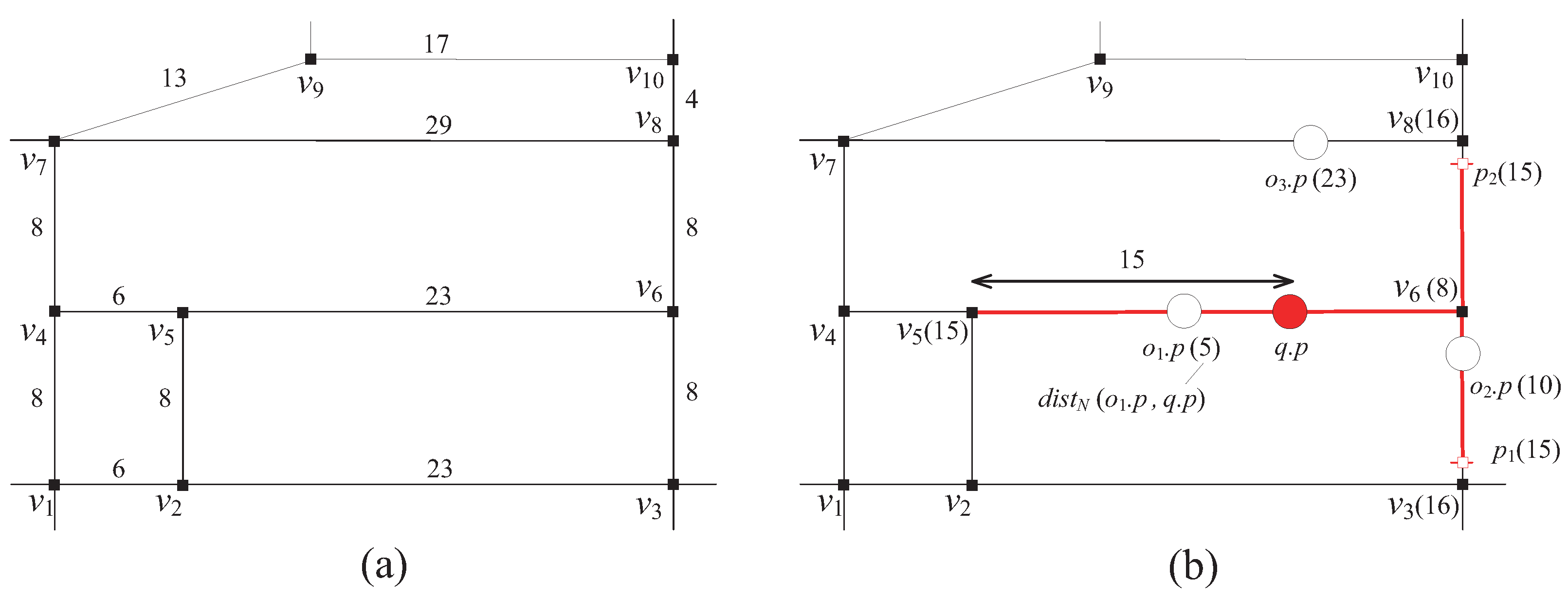
Figure 3.
System overview.
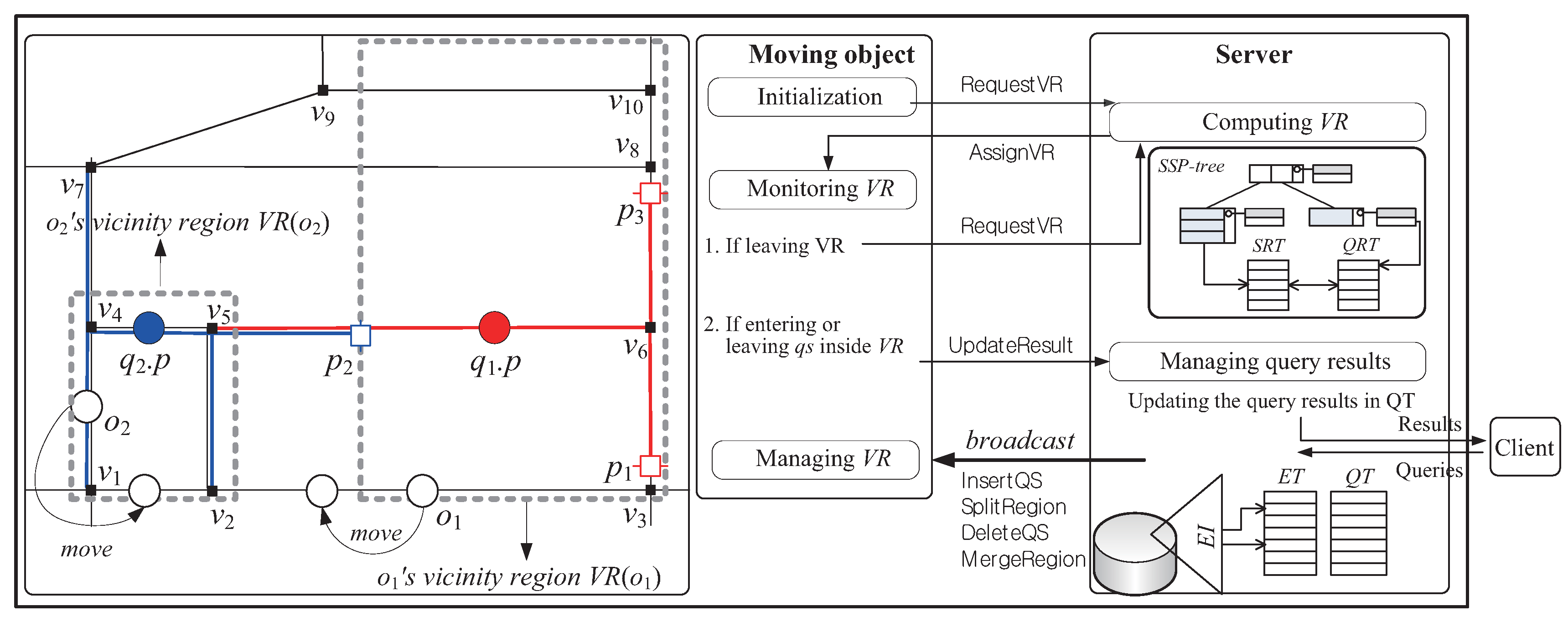
Figure 4.
Examples of approximation of query ranges and the space partitioning approach used in this paper. (a) Approximation of query ranges; (b) The space partitioning approach used in this paper.
Figure 4.
Examples of approximation of query ranges and the space partitioning approach used in this paper. (a) Approximation of query ranges; (b) The space partitioning approach used in this paper.
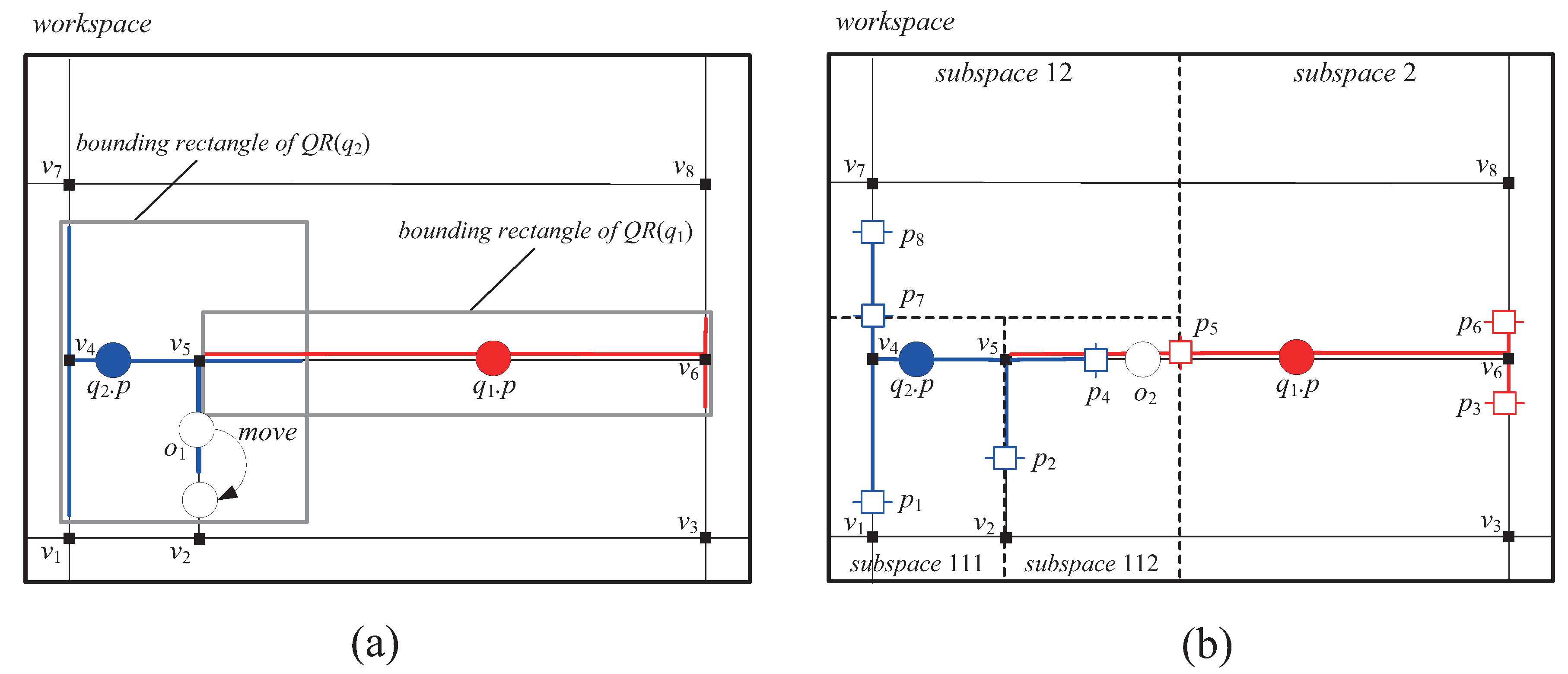
Figure 5.
Simple intersection relationships between and N. (a) is inside N or N contains ; (b) partially intersects N or vice versa; (c) fully intersects N or vice versa.
Figure 5.
Simple intersection relationships between and N. (a) is inside N or N contains ; (b) partially intersects N or vice versa; (c) fully intersects N or vice versa.

Figure 6.
An example of the SSP-tree.
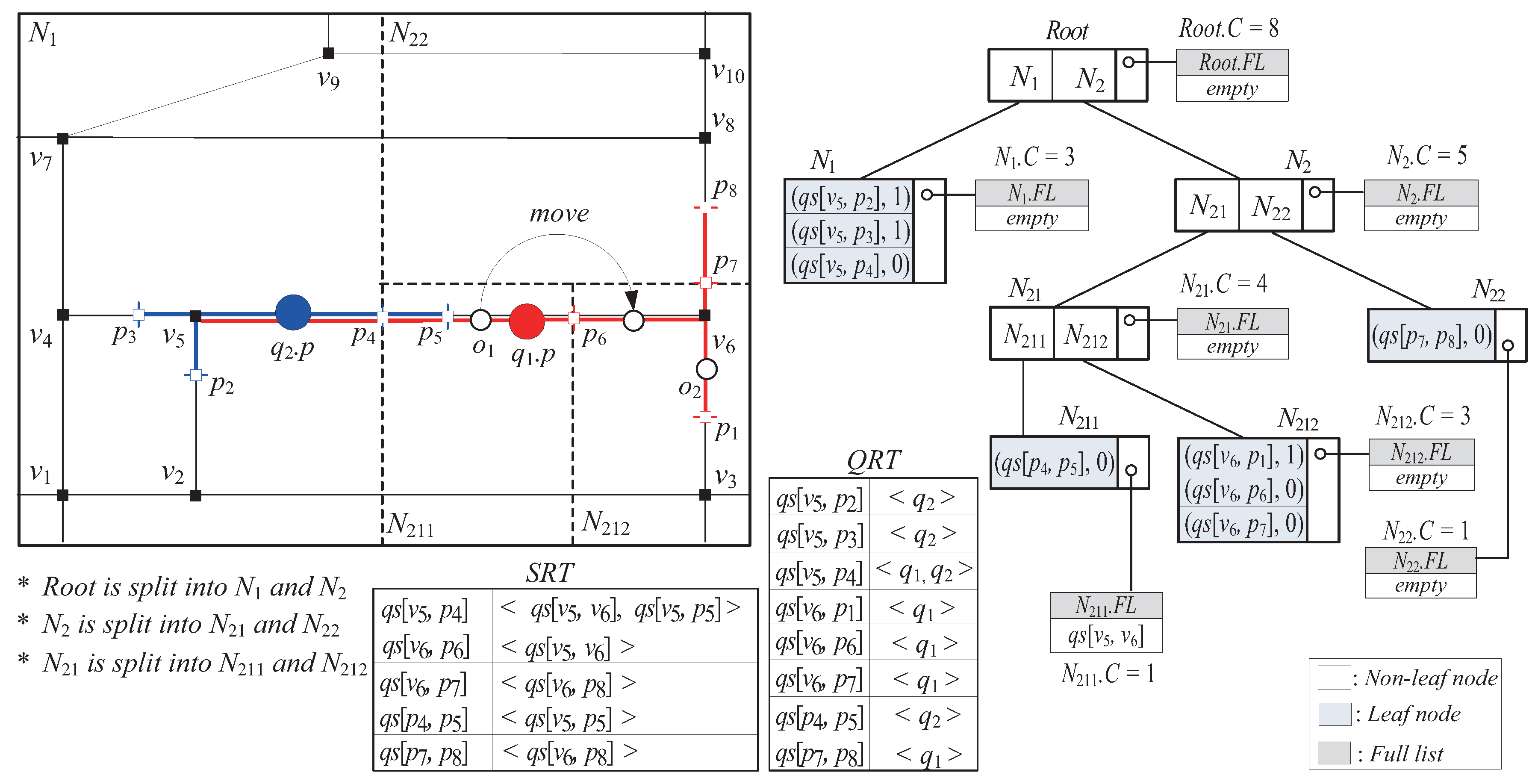
Figure 7.
Effect of the number of queries on the communication cost and the server computation cost. (a) Total number of messages vs. the number of queries; (b) The amount of CPU-time vs. the number of queries.
Figure 7.
Effect of the number of queries on the communication cost and the server computation cost. (a) Total number of messages vs. the number of queries; (b) The amount of CPU-time vs. the number of queries.
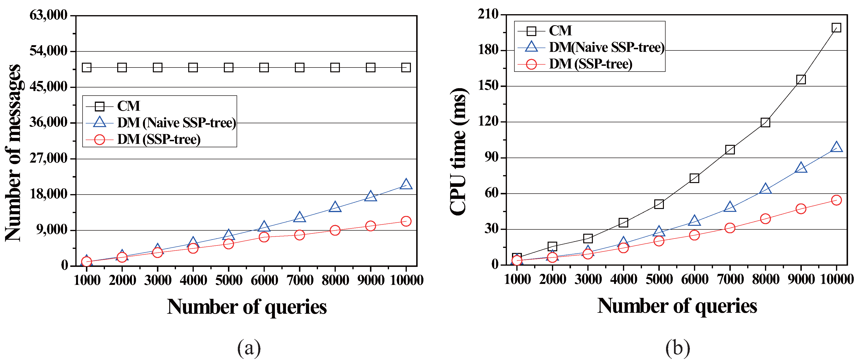
Figure 8.
Effect of the query distance on the communication cost and the server computation cost. (a) Total number of messages vs. the query distance; (b) The amount of CPU-time vs. the query distance.
Figure 8.
Effect of the query distance on the communication cost and the server computation cost. (a) Total number of messages vs. the query distance; (b) The amount of CPU-time vs. the query distance.
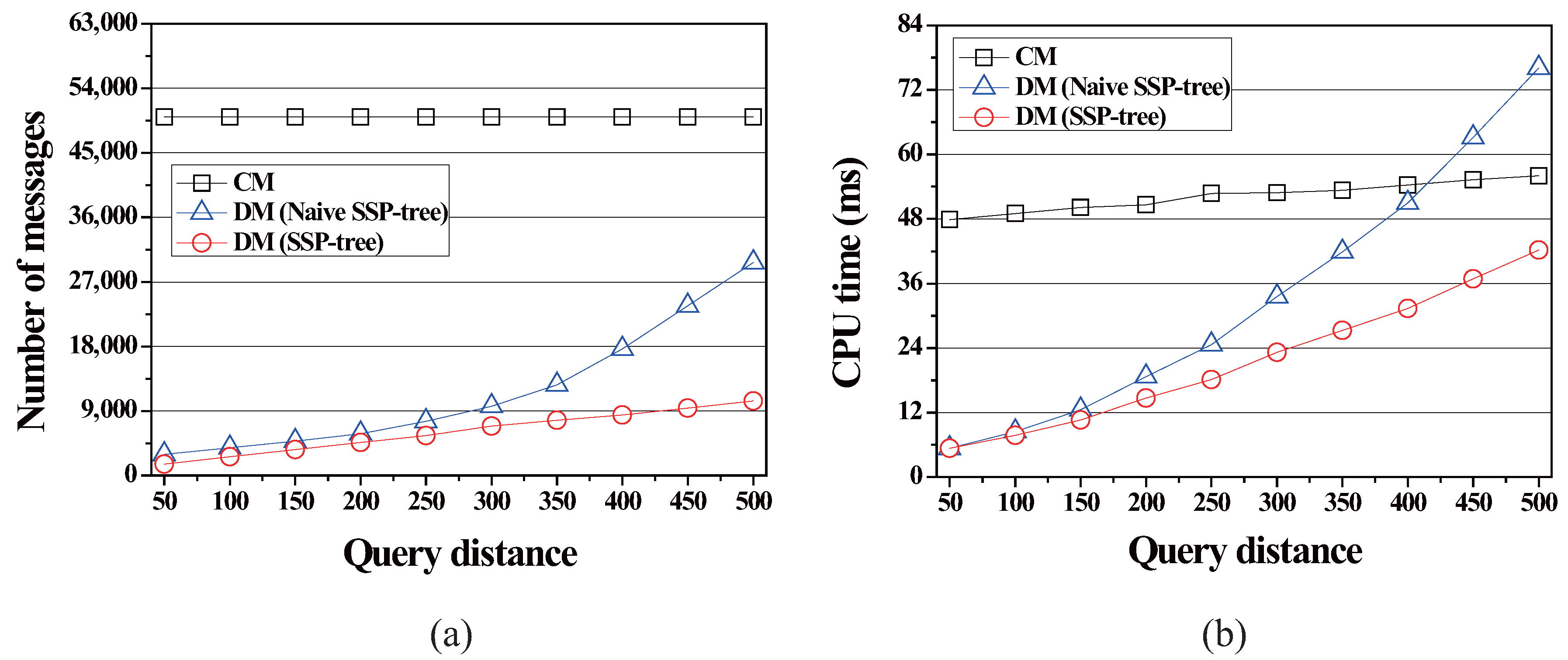
Figure 9.
Effect of the number of moving objects on the communication cost and the server computation cost. (a) Total number of messages vs. the number of moving objects; (b) The amount of CPU-time vs. the number of moving objects.
Figure 9.
Effect of the number of moving objects on the communication cost and the server computation cost. (a) Total number of messages vs. the number of moving objects; (b) The amount of CPU-time vs. the number of moving objects.

Figure 10.
Effect of the minimum computational capability on the communication cost and the server computation cost. (a) Total number of messages vs. the minimum computational capability; (b) The amount of CPU-time vs. the minimum computational capability.
Figure 10.
Effect of the minimum computational capability on the communication cost and the server computation cost. (a) Total number of messages vs. the minimum computational capability; (b) The amount of CPU-time vs. the minimum computational capability.

Figure 11.
Construction time of the SSP-tree and CPU-time consumed by a moving object. (a) Construction time of the SSP-tree vs. the number of queries; (b) The amount of CPU-time consumed by a moving object in DM vs. the minimum computational capability; all other parameters have their default values (see the values stated in boldface in Table 2).
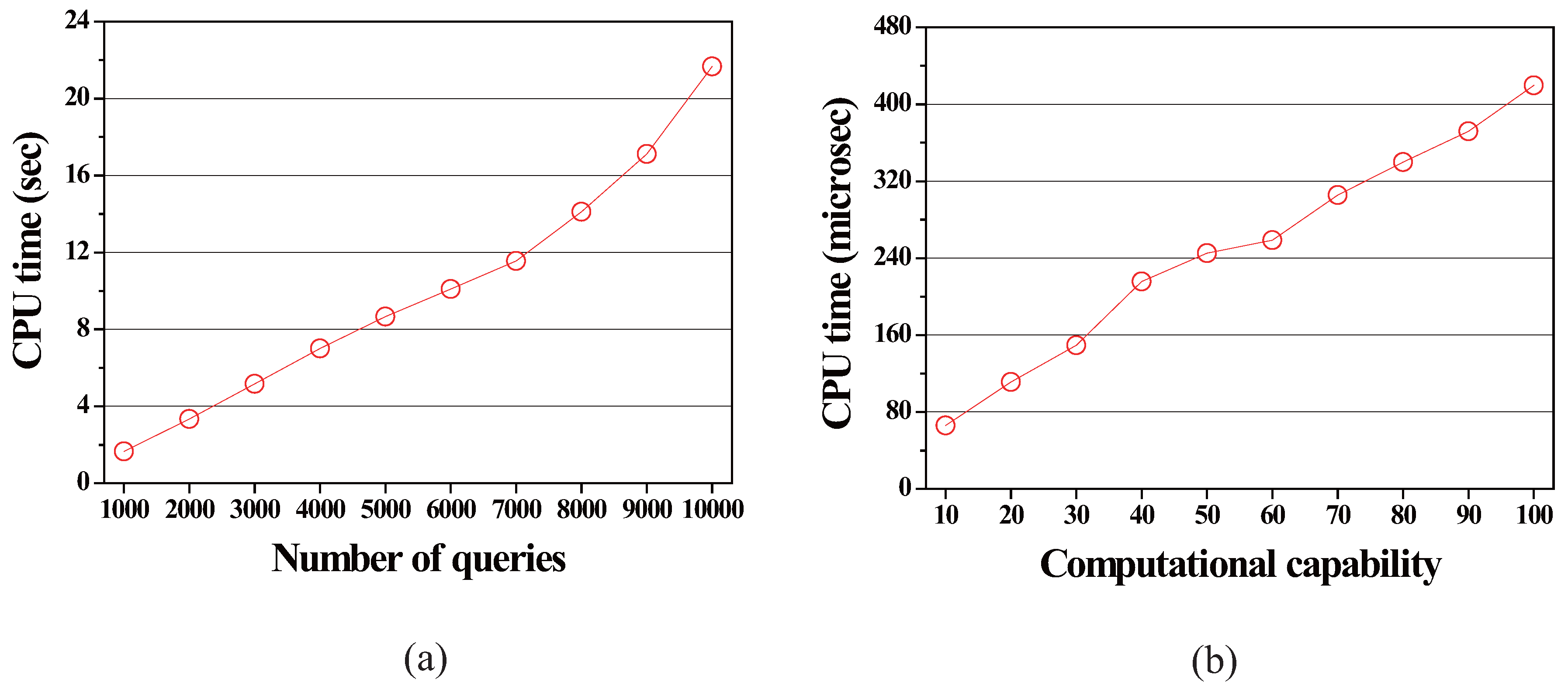

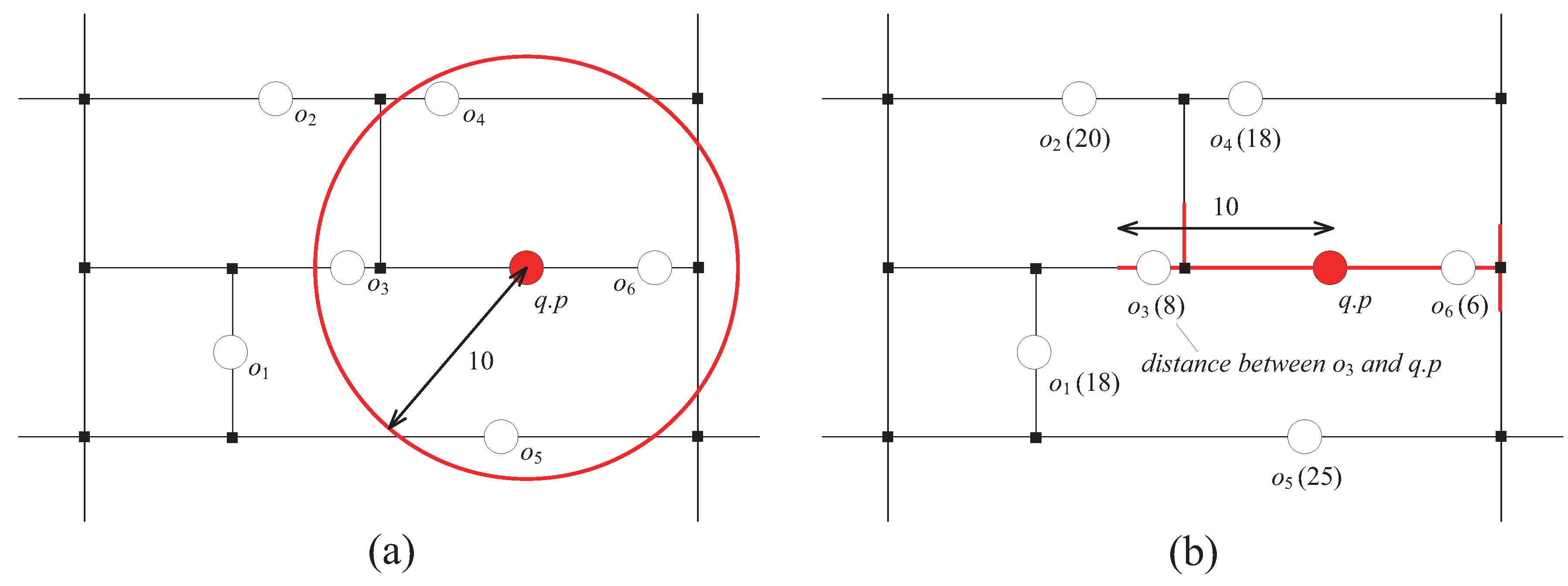
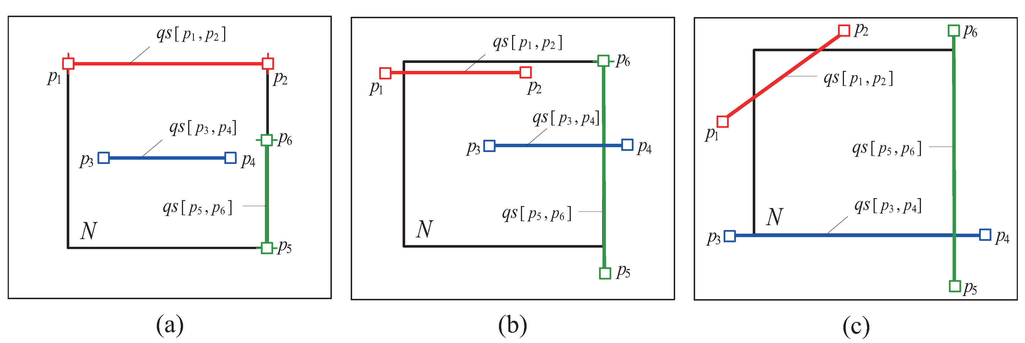
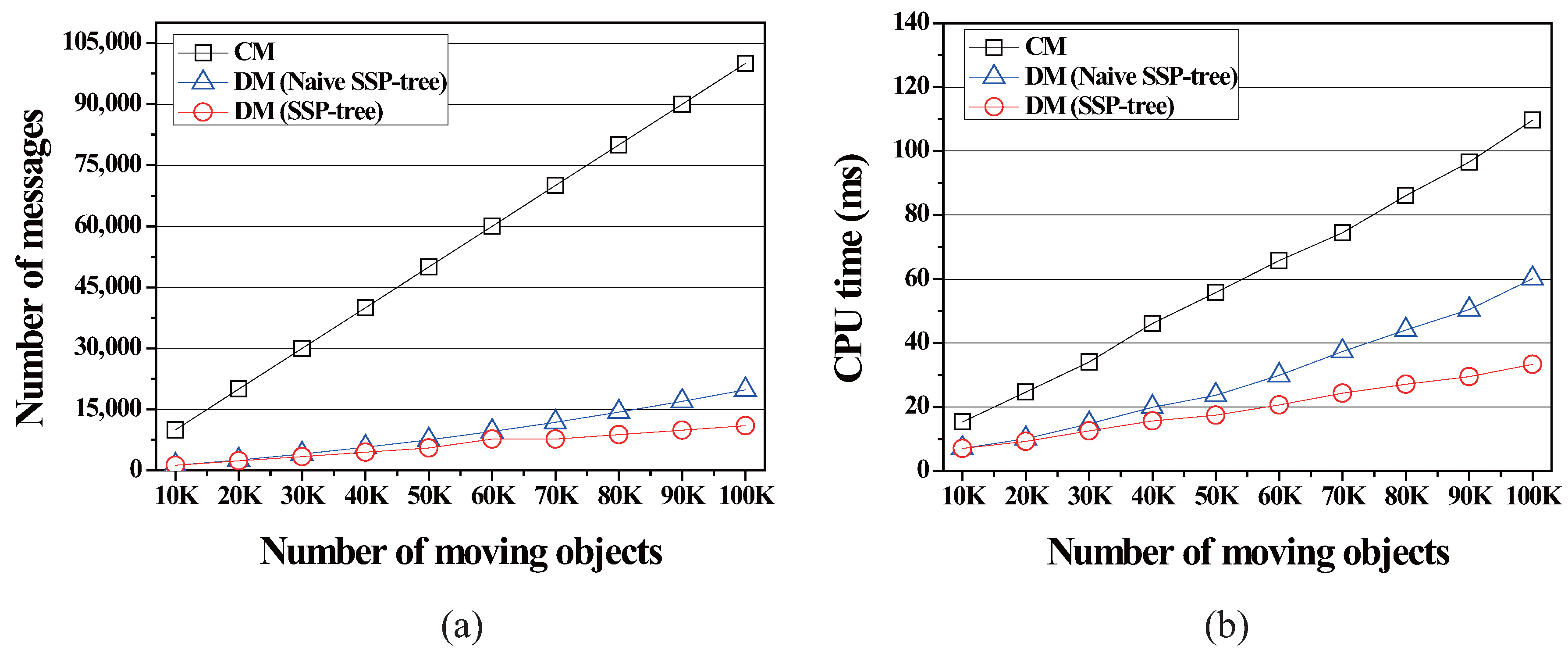
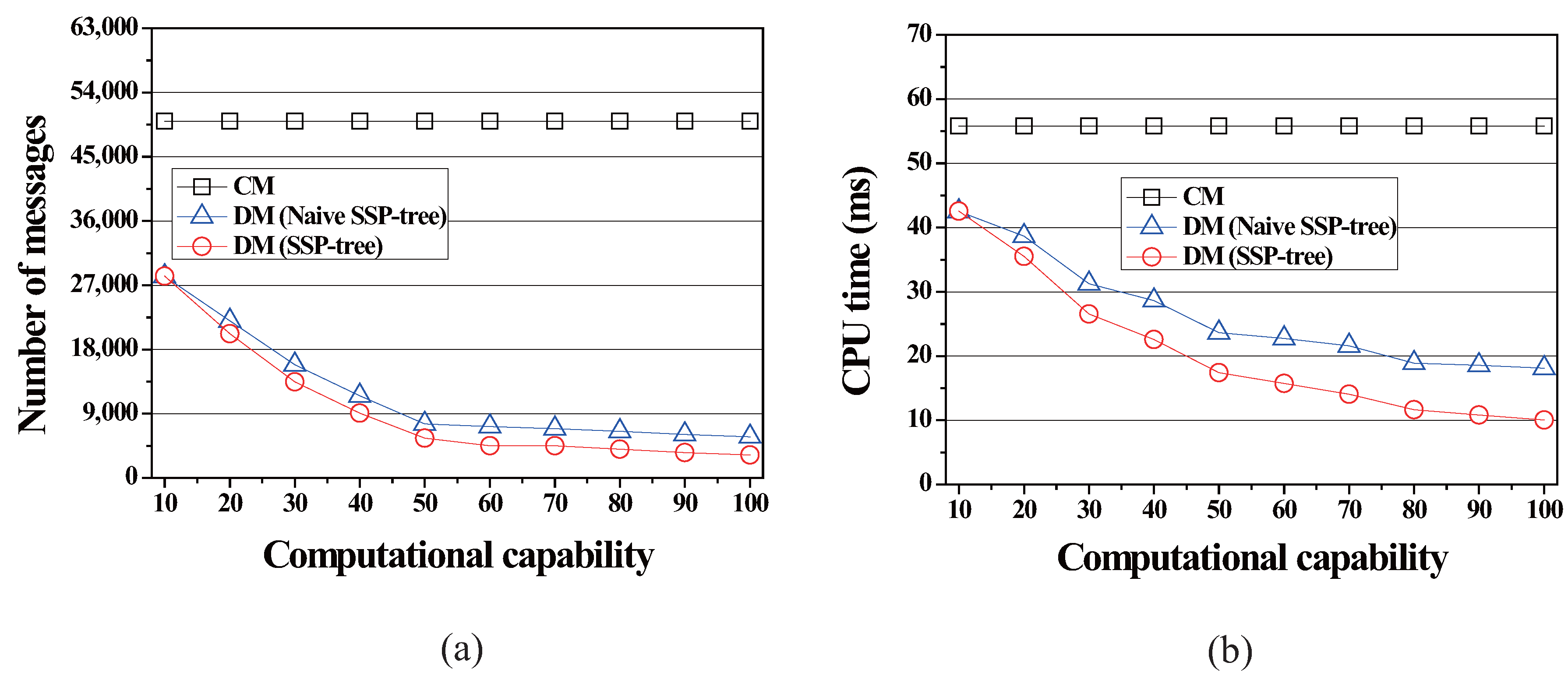
Table 1.
Frequently used notation.
| Notation | Explanation |
|---|---|
| A graph model of the road network (V: a set of vertices, E: a set of edges) | |
| A vertex in G | |
| or e | An edge in G |
| o | A moving object |
| The point of o’s current location | |
| o’s computational capability | |
| A range monitoring query (: query point, : query distance) | |
| The query range of q | |
| or (of q) | A query segment (of q) |
| The Euclidean distance between any two points in G | |
| The network distance between any two points in G | |
| N | A SSP-tree node or its corresponding subspace |
| The count variable maintained in N | |
| The full list maintained in N | |
| Query relevance table | |
| Segment relevance table |
Table 2.
Simulation parameters and their values.
| Simulation Parameter | Value Used (Default) |
|---|---|
| Number of queries | 1000∼10,000 (5000) |
| Query distance | 50∼500 (250) |
| Number of moving objects | 10,000∼100,000 (50,000) |
| Minimum computational capability | 10∼100 (50) |
© 2017 by the authors. Licensee MDPI, Basel, Switzerland. This article is an open access article distributed under the terms and conditions of the Creative Commons Attribution (CC BY) license (http://creativecommons.org/licenses/by/4.0/).
Share and Cite
MDPI and ACS Style
Jung, H.; Kim, U.-M. The SSP-Tree: A Method for Distributed Processing of Range Monitoring Queries in Road Networks. ISPRS Int. J. Geo-Inf. 2017, 6, 322. https://doi.org/10.3390/ijgi6110322
AMA Style
Jung H, Kim U-M. The SSP-Tree: A Method for Distributed Processing of Range Monitoring Queries in Road Networks. ISPRS International Journal of Geo-Information. 2017; 6(11):322. https://doi.org/10.3390/ijgi6110322
Chicago/Turabian StyleJung, HaRim, and Ung-Mo Kim. 2017. "The SSP-Tree: A Method for Distributed Processing of Range Monitoring Queries in Road Networks" ISPRS International Journal of Geo-Information 6, no. 11: 322. https://doi.org/10.3390/ijgi6110322
Note that from the first issue of 2016, this journal uses article numbers instead of page numbers. See further details here.