A Feature-Based Approach of Decision Tree Classification to Map Time Series Urban Land Use and Land Cover with Landsat 5 TM and Landsat 8 OLI in a Coastal City, China

Abstract

Accurate mapping of temporal changes in urban land use and land cover (LULC) is important for monitoring urban expansion and changes in LULC, urban planning, environmental management, and environmental modeling. In this study, we present a feature-based approach of the decision tree classification (FBA-DTC) method for mapping LULC based on spectral and topographic information. Landsat 5 TM and Land 8 OLI images were employed, and the technique was applied to the coastal city of Xiamen, China. The method integrates multi-spectral features such as SAVI (soil adjustment vegetation index), NDWI (normalized water index), MNDBaI (modified normalized difference barren index), BI (brightness index), and WI (wetness index), with topographic features including DEM and slope. In addition, the new approach distinguishes between fallow land and cropland, and separates high-rise buildings from beaches and water bodies. Several of the FBA-DTC parameters (or rules) from 1997 to 2015 remained constant (i.e., DEM and slope), whereas others changed slightly. WI was negatively related to percent area of beach land, and BI was negatively related to percent area of arable land. The FBA-DTC method had an average user’s accuracy (UA) of 91.36% for built-up land, an average overall accuracy (OA) of 92.13%, and a Kappa coefficient (KC) of 0.90 for the period from 2003 to 2015, representing respective increases of 15.87%, 10.17%, and 0.13, compared with values calculated using maximum likelihood classification (MLC). Over the past 12 years, built-up land increased from 23.67% to 43.17% owing to occupation of coastal reclamation, arable land, and forest land. The FBA-DTC method presented here is a valuable technique for evaluating urban growth and changes in LULC classification for coastal cities.

1. Introduction

Urbanization represents the territorial and socioeconomic progress of an area and is associated with the transformation of land use and land cover (LULC) types from undeveloped to developed [1]. Over recent decades, global urbanization has progressed rapidly [2]. In particular, coastal urban areas have experienced fast population explosion and dynamic economic growth. Knowledge of urban LULC types and their areal distribution is essential for coping with a variety of environmental and socioeconomic issues [3,4].

Remote sensing can provide timely and detailed views of land cover, and thus is a useful approach for monitoring the growth and spatial distribution of urban areas [5]. Since the Landsat satellite was launched in the early 1970s, medium-resolution remote sensing imagery (15–30 m resolution) such as Thematic Mapper (TM), Enhanced Thematic Mapper Plus (ETM+), Landsat Operational Land Imager (OLI), Hyperion [6], and SPOT5 [7] images, and high spatial resolution imagery (<5 m resolution) such as IKONOS, Worldview, and Quickbird data, have been widely used for examining LULC changes [8,9,10].

A variety of techniques for determining urban LULC types from satellite images have been evaluated, including maximum likelihood classification (MLC), support vector machines (SVMs) [11,12], neural network classification (NNC) [13], decision tree classification (DTC), fuzzy classification [14], spectral angle mapper (SAM) classification [15], object-based image segmentation [6], classification and regression tree (CART) analysis, the hybrid method [16], expert classification [17], etc. Among these methods, DTC has the ability to deal with non-linear relationships between features and classes [18,19], requires no assumptions regarding the distribution of input data, provides an intuitive classification structure, and can be readily incorporated with other methods [20], leading to wide applicability [18,21,22]. At present, DTC techniques have been successfully applied to a wide range of LULC classification studies [23,24] using a variety of optical and radar remote sensing data, such as Landsat 7 ETM+ [18], Landsat 5 TM [19], IRS-P6 AWiFS [20,25], and polarimetric SAR data [26].

The spatial and spectral variability of urban environments presents fundamental challenges to deriving accurate remote sensing-based products for urban areas [27]. Urban areas often exhibit spectral confusion or overlap such as the occurrence of “the same objects with different spectrum” or “different objects with the same images” (or the “salt and pepper” problem) [5], which usually gives rise to ambiguity of LULC types [19,28]. New techniques are continually being developed to effectively employ features inherent in remote sensing and ancillary data for improving LULC classification [1,29]. The Landsat 8 satellite was launched in February of 2013, but the classification accuracy of Landsat 8 OLI image data has not yet been tested using DTC.

The objective of this study was to develop a feature-based approach of decision tree classification (FBA-DTC) technique to extract time series of urban LULC information using Landsat 5 TM and Landsat 8 OLI data. The approach was applied to Xiamen city in southeastern China, and the results were evaluated and compared with MLC and similar studies. This study also provides useful information for land resource management in Xiamen city.

2. Study Area and Datasets

2.1. Study Area

Xiamen city is located on the southeast coast of Fujian Province, China. The sea naturally divides the city into two parts: Xiamen island and the mainland, comprised of four suburban districts (Jimei, Haicang, Tong’an, and Xiang’an). The core urban district (117°57′–118°15′ E and 24°24′–24°39′ N), which has an area of ~480 km², was chosen as the study area (Figure 1). The region is characterized by undulating terrain, ranging from 0 m to 379 m, and has a subtropical monsoon climate with an average annual temperature of 21 °C.

Xiamen was one of the first cities established as a special economic zone in China, and it has witnessed rapid growth, both in urban spatial extent and population, over the last two decades. It has transformed from an island city to a bay-like city, with an urban center located on the island and several satellite towns and suburban clusters in the bay and plain areas of its mainland [30]. According to national censuses, Xiamen’s population increased from 2.05 million in 2000 to 3.86 million in 2015. Rapid urbanization has caused a variety of environmental problems such as water quality deterioration, farmland shortage, eutrophication of offshore waters, flood hazards and exacerbation of the urban heat island effect [31,32,33].

Like other big cities in China, Xiamen attracts vast amount of migrants and further a number of urban villages (i.e., villages in the city) are formed because many rural villages are spatially surrounded by newly developed urban land [34]. Most of urban villages consist of overcrowded multi-story buildings from three to seven floors with narrow alleys, dark and damp conditions. The urban villages can accommodate the increasing housing demand of the migrants with low affordability. Thus, local farmers extended existing houses or built new attics with white tin on the top of the houses and then rent them to migrant workers because they could earn highly profits. Nevertheless, the attics may cause potential security risks because most of them do not meet normal construction standards. The local government is developing some plans for urban village redevelopment.

2.2. Data Collection and Processing

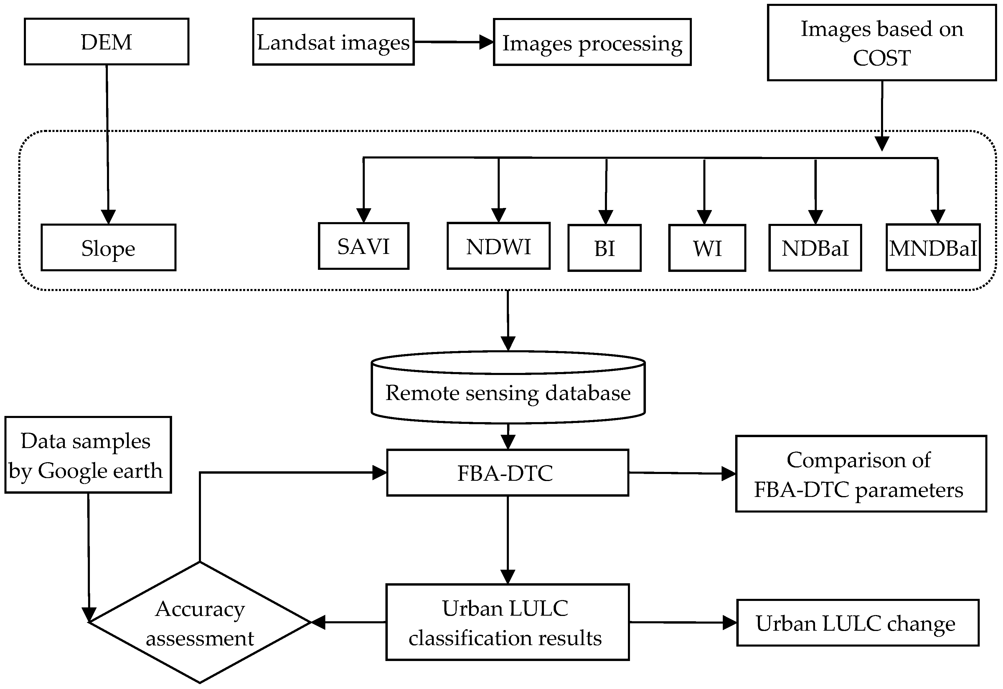
Remotely sensed data (

Table 1. Characteristics of Landsat images used in the study.

Image Type	Image Acquisition Date	Sun Elevation Angle (Degree)	Path/Row
Landsat 5 TM	28 October 2003	45.5	119/43
Landsat 5 TM	8 January 2007	36.7	119/43
Landsat 8 OLI	14 January 2015	38.0	119/43

) from Landsat 5 TM and Landsat 8 OLI images were acquired from the U.S. Geological Survey website (http://earthexplorer.usgs.gov/), and geospatial data were taken from a Computer Network Information Center, Chinese Academy of Sciences website (http://www.gscloud.cn/). The Landsat 8 satellite consists of two science instruments—Landsat 8 OLI and the Thermal Infrared Sensor (TIRS). All images used in the study were cloud-free and had excellent quality. The Landsat 8 OLI data consists of eight spectral bands, with a 30 m spatial resolution for bands 1–7 and band 9, and one panchromatic band with a 15-m resolution.

Detailed descriptions of the data sets are shown in Table 1. In addition, SRTM (Shuttle Radar Topography Mission) global digital elevation model (DEM) at 30 m resolution, and an associated slope map derived from DEM were used. All images and the DEM had the same spatial resolution (30 m) and were projected according to Universal Transverse Mercator map projection (UTM, Zone 50 N). All images were georegistered with Root Mean Squared (RMS) errors of less than 0.5 pixels. Images were preprocessed using an atmospheric correction procedure based on the COST method [35].

3. Methodology

The framework of this research is illustrated in Figure 2 and includes the following major steps: (1) COST-based atmospheric correction; (2) remote sensing database construction; (3) LULC extraction using FBA-DTC; (4) accuracy assessment; and (5) LULC change analysis.

3.1. Image-Based Atmospheric Correction

A variety of methods have been designed to reduce or remove atmospheric effects and determine land surface reflectance [36]. Examples include dark object subtraction (DOS), cosine of the solar zenith angle correction (COST) [35], and radiative transfer models (e.g., 6S and MODTRAN). The DOS model corrects for the effects of atmospheric scattering, but it ignores the effects of the atmospheric absorption. The radiative transfer models are very complex and require in situ atmospheric measurements that can be unavailable for many applications, particularly when using historical Landsat images. The COST model is based on the acquired digital image and accounts for multiplicative effects of atmospheric scattering and absorption, avoiding collecting in situ atmospheric information [35,37]. Therefore, the COST model is used for most of the remotely sensed data application, especially for the historical image data when atmospheric data are not available. It can be expressed as:

$$\rho =\frac{(L_{sat}-L_{haze})·\pi ·d^2}{ESUN·cos\theta ·TA{U}_z·TA{U}_v}$$

(1)

where ESUN is the Exo-atmospheric solar spectral irradiance; TAUv is atmospheric transmittance in the viewing direction (1.0 for Landsat images); TAUz is atmospheric transmittance in the illumination direction (cosθ for the COST method); ρ is surface reflectance; L_sat is spectral radiance at the sensor’s aperture (W/(m² ster·μm); L_haze is path radiance; θ is the solar zenith angle in degrees; and D is the normalized Earth–Sun distance.

L_sat can be expressed as:

$$L_{sat}=Gain·DN+Bias$$

(2)

where DN is the remotely sensed digital number, and Gain and Bias are the radiometric gain and bias gain for a specific band, respectively, which are provided from the header files of images.

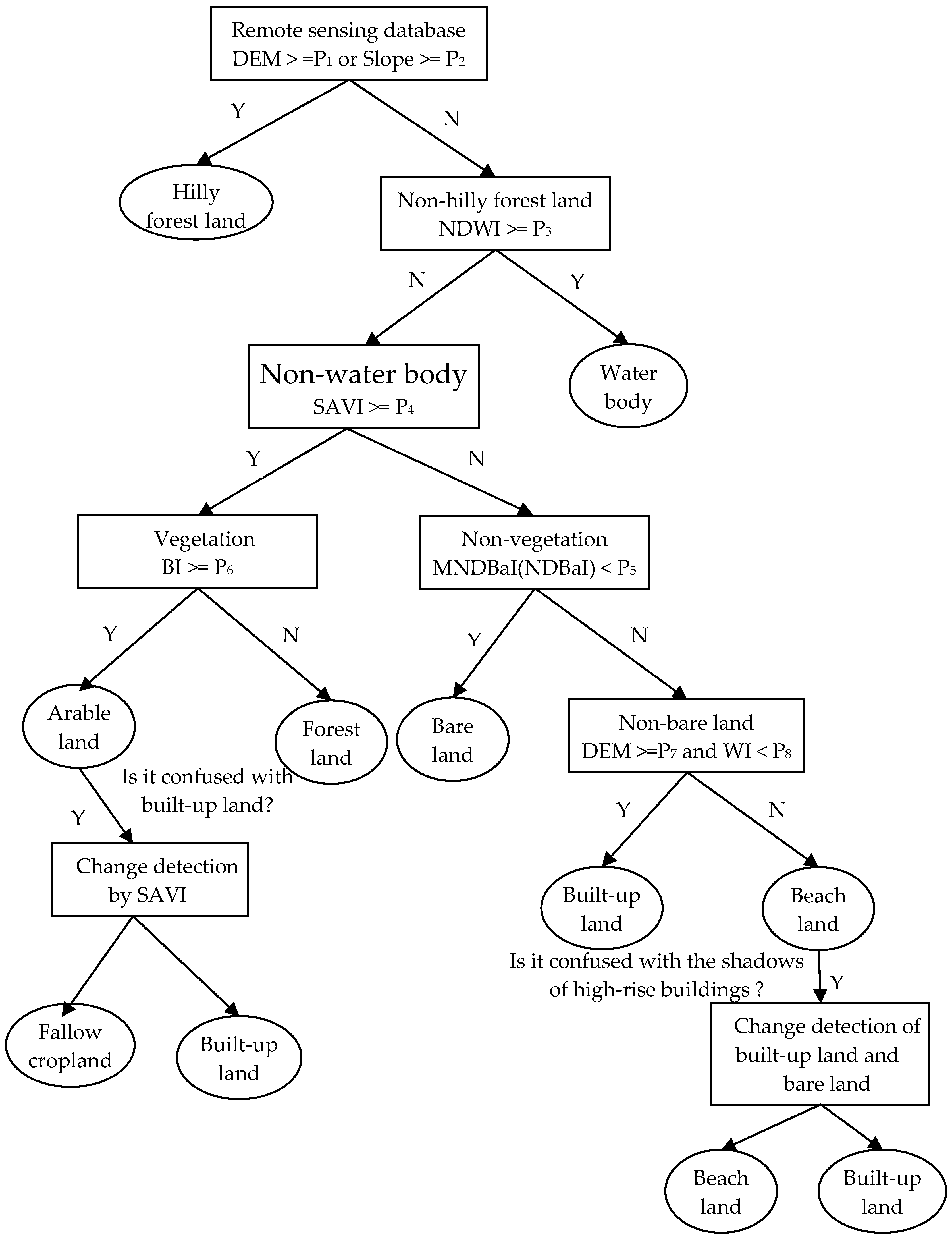
3.2. Decision Tree Classification Approach

DTC is a classification technique with a binary tree structure, which consists of a root node and a variety of internal nodes and terminal nodes (leaves). The internal nodes denote a set test or decision rules, and the leaf nodes represent detailed classes. Each internal node makes a binary decision that can distinguish a single class or several classes from the remaining classes.

Because of its flexibility, intuitive simplicity, and computational efficiency, DTC has been widely used in raster data classification and thematic information extraction, especially remote sensing data. In the DTC process, features of remote-sensing data (i.e., DEM or bands) represent predictor variables, and the LULC classes to be extracted are target variables. The target variables are derived from a series of thresholds based on the distribution of features in the feature space [19]. In this study, FBA-DTC was used to integrate multi-spectral features derived from a number of remote sensing indices such as SAVI (soil adjustment vegetation index), NDWI (normalized difference water index), MNDBaI (modified normalized difference barren index), BI (brightness index), and WI (wetness index) with topographic features including DEM and slope. The FBA-DTC approach to extracting LULC type based on multi-features was developed as shown in Figure 3. According to our research objectives and a field survey, LULC in the study area consists of six classes: arable land (AL), forest land (FL), beach land (BEL), built-up land (BU), water bodies (WB), and bare land (BL).

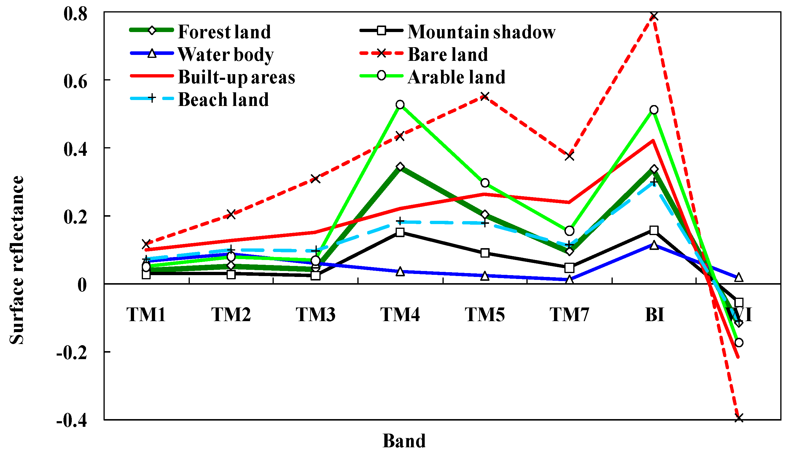
3.2.1. Vegetation Index

Huete [38] proposed SAVI to extract vegetation based on a modified normalized difference vegetation index (NDVI):

$$SAVI=({\rho }_{NIR}-{\rho }_{Red})(1+l)/({\rho }_{NIR}+{\rho }_{Red}+l)$$

(3)

where ρ_NIR and ρ_Red are the spectral reflectance of the red and near-infrared bands, respectively, for the Landsat 5 TM and Landsat 8 OLI (TM/OLI); and l is a soil-adjusted factor with a value between 0 and 1. The default l value of 0.5 can work well in most situations [38]. Equation (3) produces values in the range from −1 to 1, where positive values indicate vegetated areas and negative values signify non-vegetated surface features such as water, barren land, clouds, and snow.

3.2.2. Water Index

McFeeters [39] presented NDWI to delineate open water features:

$$NDWI=({\rho }_{Green}-{\rho }_{NIR})/({\rho }_{Green}+{\rho }_{NIR})$$

(4)

where ρ_Green and ρ_NIR are the spectral reflectance of the green and near infrared bands for TM/OLI images, respectively.

3.2.3. Bare Land Index

Zhao and Chen [40] proposed the Normalized Difference Bare Index (NDBaI) for bare land (i.e., land under development):

$$NDBaI=(d_{SWRI1}-d_{TIR})/(d_{SWRI1}+d_{TIR})$$

(5)

where d_SWRI1 and d_TIR are the raw digital numbers of the TM short-wave infrared (SWIR) 1 and thermal infrared bands, respectively.

However, we found NDBaI could not distinguish white tin roofs in urban villages from bare land. With the dramatic urbanization, a vast area of buildings with bright roofs in Xiamen has sprung up in recent years. Most of them may be posed by new attics built with white tin on top of the original houses. Figure 4 showed the significant changes of white tin roofs from 2003 to 2014 in two urban villages, Gaolin and Wutong in Xiamen island. Therefore, we used a modified normalized difference bare index (MNDBaI) for bare land in cities in which a number of the white roofs exist. The equation can be expressed as follows:

$$MNDBaI=({\rho }_{Red}-{\rho }_{Blue})/({\rho }_{Red}+{\rho }_{Blue})$$

(6)

where ρ_Red and ρ_Blue are the spectral reflectance of red and blue bands for TM/OLI images, respectively.

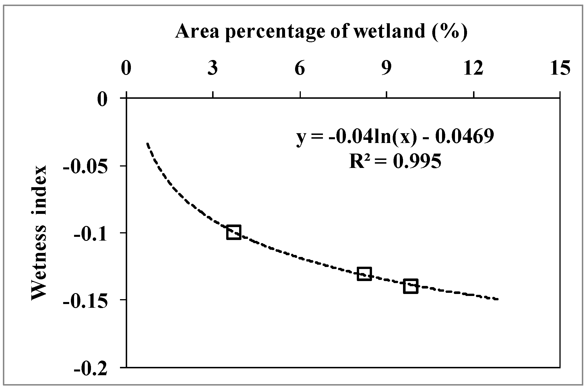
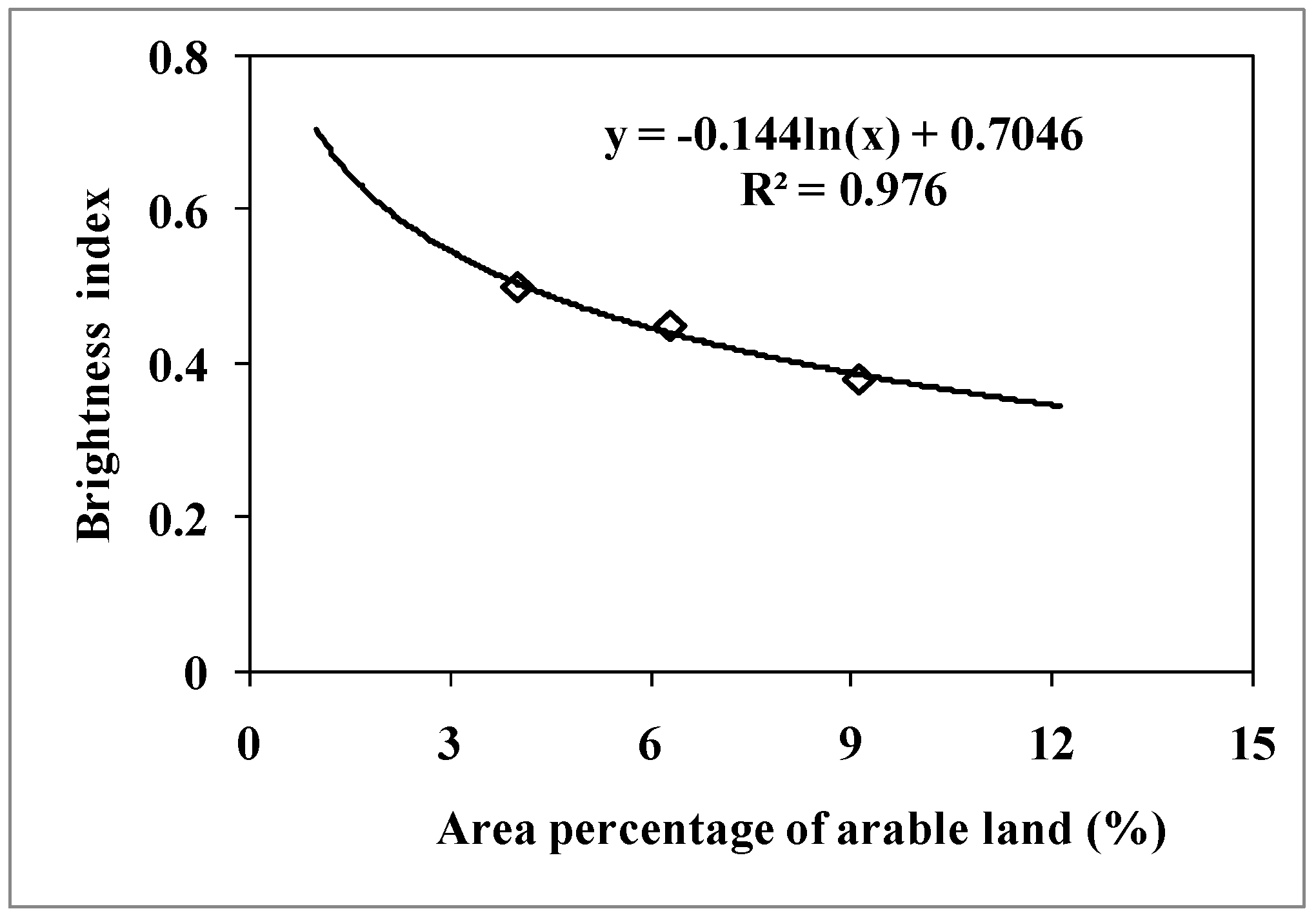
3.2.4. Brightness Index and Wetness Index

The tasseled-cap transformation was originally defined by Kauth and Thomas [41] (1976), who analyzed the spectra of wheat growth using Landsat MSS. The transformation is executed by taking linear combinations of the original or reflected image bands. In addition to Landsat Multispectral Scanner MSS, transformation coefficients have been derived for Landsat 5 TM, ETM+, IKONOS, Landsat 8 OLI, etc.

The brightness index (BI), the first tasseled-cap band, corresponds to the overall brightness of an image. Cropland typically has a higher brightness value than forest land (Figure 5).

Beaches are one of the most important land-use types in coastal cities, but it is difficult to separate beaches from built-up land because of their similar spectral characteristics. The wetness index (WI), the third tasseled-cap band, is typically used as an index of “wetness” (e.g., soil or surface moisture). Compared with the spectral characteristics of built-up land, beaches have a high WI and low terrain. Thus, they can be distinguished from built-up land by combining image analysis with elevation information. Tasseled cap transformation reflectance coefficients for TM and OLI images were cited from Crist [42] and Baig et al. [43], respectively:

$$B{I}_{TM}=0.2043{\rho }_{Blue}+0.4158{\rho }_{Green}+0.5524{\rho }_{Red}+0.5741{\rho }_{NIR}+0.3124{\rho }_{SWIR1}+0.2303{\rho }_{SWIR2}$$

(7)

$$W{I}_{TM}=0.0315{\rho }_{Blue}+0.2021{\rho }_{Green}+0.3102{\rho }_{Red}+0.1594{\rho }_{NIR}-0.6806{\rho }_{SWIR1}-0.6109{\rho }_{SWIR2}$$

(8)

$$B{I}_{OLI}=0.3029{\rho }_{Blue}+0.2786{\rho }_{Green}+0.4733{\rho }_{Red}+0.5599{\rho }_{NIR}+0.508{\rho }_{SWIR1}+0.1872{\rho }_{SWIR2}$$

(9)

$$W{I}_{OLI}=0.1511{\rho }_{Blue}+0.1973{\rho }_{Green}+0.3283{\rho }_{Red}+0.3407{\rho }_{NIR}-0.7117{\rho }_{SWIR1}-0.4559{\rho }_{SWIR2}$$

(10)

where, ρ_Green, ρ_Blue, ρ_Red, ρ_NIR, ρ_SWIR1, and ρ_SWIR2 are spectral reflectance values in the TM/OLI blue, green, red, near infrared, short-wave infrared 1 (SWIR1), and short-wave infrared 2 (SWIR2) bands, respectively; BI_TM and WI_TM represent the brightness index and wetness index for Landsat 5 TM, respectively; and BI_OLI and WI_OLI represent the brightness index and wetness index for Landsat 8 OLI, respectively.

3.2.5. FBA-DTC Procedure

As shown in Figure 3, DEM and slope first are used to partition all pixels into two groups. The spectral characteristics of forests shadowed by mountains are similar to those of water bodies (Figure 5). However, certain forests typically grow above certain elevations or slopes, particularly in Xiamen. Therefore, topographic features can be used to distinguish mountain-shaded forests from other classes such as built-up land, water, and other vegetation types. NDWI is used to distinguish water from other classes because water has a higher NDWI value than that of other classes. SAVI can be employed to separate vegetated areas (forest and cropland) from non-vegetated areas (built-up land, bare land, and beaches). BI is helpful for distinguishing between forests and cropland because cropland corresponds to a higher BI value compared with forests.

The spectra of beach land and built-up land are similar (Figure 5), but DEM and WI are helpful for distinguishing between the two. Built-up land typically exists at higher elevation compared with beaches. However, due to the rapid expansion of urban space and population growth, more and more beach areas, and even the surrounding sea, are being urbanized. Thus, WI is employed in combination with DEM to distinguish between beaches and build-up land with the similar elevation, as beaches have a higher WI value than that of built-up land.

NDBaI or MNDBaI can be used to distinguish bare land from beaches and built-up land. However, MNDBaI cannot be used to distinguish fallow land from bare land and NDBaI cannot be used to extract the buildings with white tin roofs. Thus, we used NDBaI for images from 2003 to MNDBaI for those from 2007 to 2015.

During certain seasons, both fallow land and cropland (Figure 6) exist simultaneously, thereby confounding the extraction of these two land types. For example, Xiang’an district is one of the biggest carrot planting and export bases in China because the district has suitable climate and great sandy soil for the growth of carrots. Carrots in the district are usually planted during September and October and harvested during May and June each year. Figure 6 shows distinctly different spectral response characteristics of lands in carrot farming on 28 October (a) and 8 January (b), respectively. In Figure 6a, yellow means very young leaves of carrots planted in October and pink means middle-aged leaves of carrots planted in September. In Figure 6b, bright red means mature leaves of carrots that have grown for approximately 3 months. Furthermore, fallow land often is confused with built-up land. To solve this issue, it is critical to compare SAVI (via subtraction) for two images from different seasons (i.e., one image in which either fallow land or cropland exist and another in which both are present).

With the explosive population growth in Xiamen, high-rise buildings with 18 floors or more have dramatically increased to accommodate the increased population. The spectral features of such buildings are very similar to those of beaches and water, and cannot be easily distinguished. However, high-rise buildings often are built over three years and may arise from previous low-rise buildings or bare land. If bare land or built-up land from an early image (e.g., in 2007) is identified as a beach or water body in subsequent imagery (e.g., in 2015), this indicates that the latter classification is likely incorrect. Therefore, we can detect the conversion of bare land to built-up land by comparing different images.

3.2.6. Calibration of FBA-DTC Parameters

After all images were corrected for atmospheric effects using the COST method, and a dataset for each image, including SAVI, NDWI, MNDBaI (or NDBaI), BI, and WI values, were produced (Equations (3)–(10)).

We collected a minimum of 15 training sites for each LULC class in each Landsat scene processed by the COST model from 2003 to 2015. The training sites were redefined or added using Google Earth (GE) images with the close acquisition dates as the original remotely sensed data. The size per training site in the images ranged from 12 to 630 pixels. We could calculate a minimum pixel value in each image (the dataset, DEM, Slope, etc.) in training sites of its corresponding LULC class according to Figure 3, respectively. The minimum pixel values were the parameters in Figure 3. For example, the parameter P₂ in Figure 3 was the minimum pixel value of NDWI image in training sites for water body. Thus, we achieved an initial set of parameters of FBA-DTC. The parameters were further re-examined and modified based on LULC class accuracies wherever necessary till a satisfactory product was attained.

3.3. Accuracy Assessment

Although ground data are required for accuracy assessments, such data are sometimes difficult and expensive to obtain, particularly historical data. Therefore, it is acceptable for high spatial resolution images and large-scale maps to be used as reference data [16]. In this study, independent ground samples were collected from GE images and used as reference data. GE provides free access to high-resolution satellite imagery. In addition to being used as “pictures” for visualization, GE has been recognized as a significant resource for ground-truth data [44], improving visual interpretation, and even classifying complex LULC types [45]. In order to obtain better reference data, the time stamps of the GE images we chose were as close as possible to those of the original images (2 March 2003, 5 December 2006, and 30 December 2014).

It has been suggested that a minimum 50 samples (or pixels) of each class should be included in error analyses [16]. Here we used at least 60 samples for each class. For each scene, 800 samples were randomly selected using a stratified random sampling scheme and exported to GE for accuracy assessment. The classification results were evaluated based on a confusion matrix. Four validation metrics, kappa coefficient (KC), overall accuracy (OA), producer’s accuracy (PA), and user’s accuracy (UA), were determined from the matrix. UA is the inverse of the error of commission, i.e., UA = 1 − commission error, and PA is the inverse of the error of omission, i.e., PA = 1 − omission error.

To evaluate the performance of the proposed FBA-DTC, a supervised maximum likelihood classification (MLC) method was conducted for the three Landsat images, resulting in three LULC maps.

4. Results and Discussion

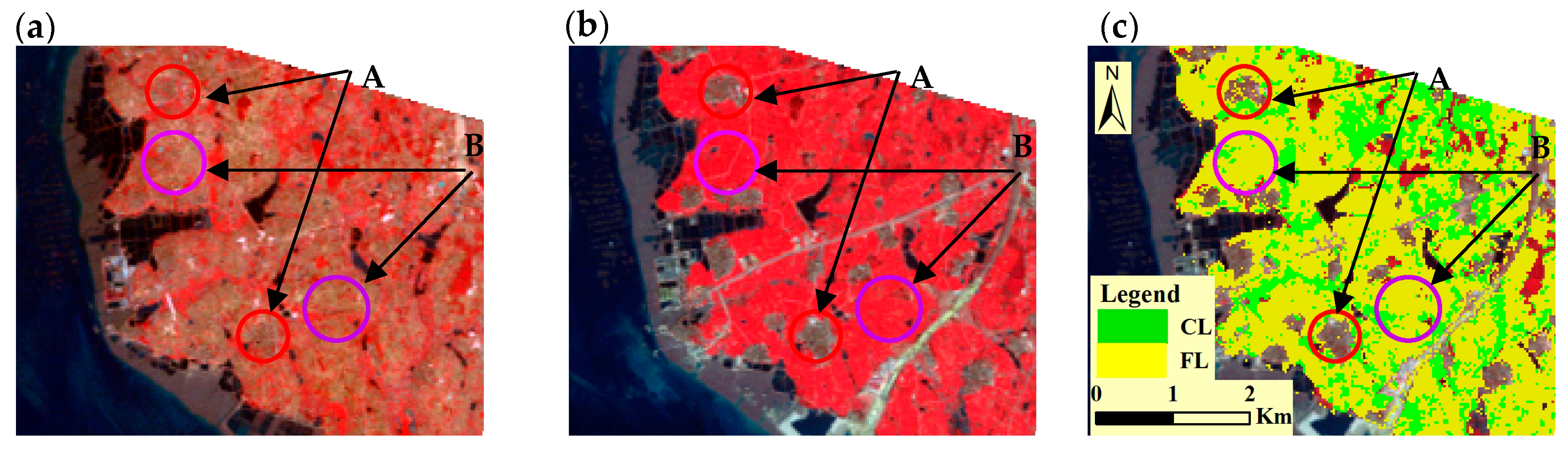
4.1. FBA-DTC Results

Extraction of LULC was carried out using DTC based on this dataset, DEM, and slope.

Table 2. Parameters of feature-based approach of decision tree classification derived from the images in Xiamen.

Year	DEM (P1)	Slope (P2)	NDWI (P3)	SAVI (P4)	MNDBaI (P5)	MNDBaI (P5)	BI (P6)	DEM (P7)	WI (P8)
2003	112	10	−0.1	0.28		−0.05	0.38	6	−0.13
2007	112	10	−0.1	0.31	0.33		0.45	6	−0.14
2015	112	10	0	0.31	0.39		0.50	6	−0.10

See Figure 4 for key to abbreviations.

shows the parameters values derived from the dataset, DEM, and slope from 2003 to 2015. Some FBA-DTC parameters were constant, such as elevation and slope, and others only varied slightly. Built-up land was located in areas below 112 m elevation with a slope of <10 degrees.

Figure 7 shows the relationship between WI and percent area of beaches. WI decreased with increasing beach area. Though beaches and even water bodies in Xiamen have been urbanized, sea level has a huge impact on beach area. Larger beach area corresponds to higher sea levels (e.g., in 2015). During the study period in Xiamen, beach area first increased, and then decreased; thus, WI values showed the opposite trend.

Figure 8 shows the relationship between BI and percent area of arable land. BI decreased with increasing area of arable land, and the trend was stronger than that for WI. Urban sprawl has occupied a large area of arable land, leading to reducing arable land yearly. Therefore, BI increased from 2003 to 2015.

4.2. Analysis of Classification Accuracy and Other Similar Studies

Table 3. Accuracy assessment of feature-based approach of decision tree classification (FBA-DTC) and maximum likelihood classification for the 2015 image.

Classified	Classified	Reference			Data
Method	Data	FL	AL	WB	Beach	BUA	BL	Total	UA (%)
FBA-DTC	FL	122	1	0	0	7	1	131	93.13
	AL	7	58	0	0	3	2	70	82.86
	WB	0	0	203	1	1	0	205	99.02
	Beach	0	0	4	62	2	0	68	91.18
	BUA	6	0	2	1	249	8	266	93.61
	BL	1	3	0	0	3	53	60	88.33
	Total	136	62	209	64	265	64	800
	PA (%)	89.71	93.55	97.13	96.88	93.96	82.81
MLC	FL	71	0	0	0	0	0	71	100.00
	AL	5	51	0	0	1	1	58	87.93
	WB	0	0	175	0	0	0	175	100.00
	Beach	0	0	0	35	1	0	36	97.22
	BUA	59	9	34	29	250	8	389	64.27
	BL	1	2	0	0	13	55	71	77.46
	Total	136	62	209	64	265	64
	PA (%)	52.21	82.26	83.73	54.69	94.34	85.94

Note: FL, forest land; AL, arable land; WB, water body; BUA, built-up land; BL, bare land; PA, producer’s accuracy; UA, user’s accuracy.

,

Table 4. Accuracy assessment of feature-based approach of decision tree classification (FBA-DTC) and maximum likelihood classification for the 2007 image. (See Table 3 for key to abbreviations).

Classified	Classified	Reference			Data
Method	Data	FL	AL	WB	Beach	BUA	BL	Total	UA (%)
FBA-DTC	FL	131	2	0	0	1	0	134	97.76
	AL	8	60	0	0	3	3	74	81.08
	WB	0	0	202	0	0	0	202	100.00
	Beach	0	0	20	73	1	0	94	77.66
	BUA	6	2	4	1	215	8	236	91.10
	BL	1	1	0	0	0	58	60	96.67
	Total	146	65	226	74	220	69	800
	PA (%)	89.73	92.31	89.38	98.65	97.73	84.06
MLC	FL	117	7	0	0	1	0	125	93.60
	AL	6	55	0	0	2	2	65	84.62
	WB	0	0	196	5	0	0	201	97.51
	Beach	0	0	5	62	0	0	67	92.54
	BUA	22	2	24	7	212	14	281	75.44
	BL	1	1	1	0	5	53	61	86.89
	Total	146	65	226	74	220	69	800
	PA (%)	80.14	84.62	86.73	83.78	96.36	76.81

,

Table 5. Accuracy assessment of feature-based approach of decision tree classification (FBA-DTC) and maximum likelihood classification for the 2003 image.

Classified	Classified	Reference			Data
Method	Data	FL	AL	WB	Beach	BUA	BL	Total	UA (%)
FBA-DTC	FL	133	4	0	0	7	2	146	91.10
	AL	10	73	2	0	6	5	96	76.04
	WB	0	0	217	2	0	0	219	99.09
	Beach	0	0	15	75	1	0	91	82.42
	BUA	7	2	4	0	168	7	188	89.36
	BL	0	0	0	0	1	59	60	98.33
	Total	150	79	238	77	183	73	800
	PA (%)	88.67	92.41	91.18	97.40	91.80	80.82
MLC	FL	85	0	12	8	0	0	105	80.95
	AL	56	76	4	0	14	7	157	48.41
	WB	1	0	191	0	0	0	192	99.48
	Beach	0	0	21	66	0	0	87	75.86
	BUA	4	1	10	3	157	6	181	86.74
	BL	4	2	0	0	12	60	78	76.92
	Total	150	79	238	77	183	73	800
	PA (%)	56.67	96.20	80.25	85.71	85.79	82.19

See Table 3 for key to abbreviations.

and

Table 6. Summary of major studies employing decision tree classification methods.

Authors	Data Types	Methods	LULC Classes	OA (%)	KC	Increased OA (%)	Increased KC
Pal and Mather [18]	Landsat 7 ETM+	Boosted DTC	7	88.46	0.87	5.56	0.07
		MLC	7	82.90	0.80
Kandrika and Roy [25]	IRS-P6 AWiFS	DTC (See-5)	16	87.50	0.87
Punia et al. [20]	IRS-P6 AWiFS	DTC (See-5)	11	91.81
Qi et al. [26]	PolSAR	DTC-OOC	7	86.64	0.84	16.98	0.19
		MLC	7	69.66	0.65
Wang et al. [19]	Landsat	DTC	7	95.87	-	4.44	-
	5 TM	MLC	7	91.43	-
Hua et al. (this paper)	Landsat	FBA-DTC	6	90.63	0.88	11.25	0.14
	5 TM/2003	MLC	6	79.38	0.74
	Landsat	FBA-DTC		92.38	0.90	5.50	0.07
	5 TM/2007	MLC	6	86.88	0.83
	Landsat 8	FBA-DTC		93.38	0.92	13.75	0.19
	OLI/2015	MLC		79.63	0.73

Note: DTC, decision tree classification; See-5, a commercially available decision tree algorithm; DTC-OOC, decision tree classification combined with object-oriented classification; feature-based approach of decision tree classification (FBA-DTC); MLC, maximum likelihood classification; OA, overall accuracy; KC, kappa coefficient.

summarize the accuracy assessment for LULC classification based on FBA-DTC and MLC. Figure 9 shows spatio-temporal changes in LULC distributions derived from DTC and MLC classification results. Based on the overall accuracies of the error matrices, the OA values for the FBA-DTC results were 90.63%, 92.38%, and 93.38% in 2003, 2007, and 2015, respectively, much higher than those for MLC (79.38%, 86.88%, and 79.63% for corresponding years). The KC values for the FBA-DTC results were 0.88, 0.90, and 0.92 in 2003, 2007, and 2015, respectively, whereas those for MLC were 0.74, 0.83, and 0.73. The FBA-DTC method produced a high average OA value of 92.13% and a KC value of 0.90. The average OA and KC values increased by 10.17% and 0.13 compared with corresponding values for MLC. Thus, the proposed method produced more accurate results compared with MLC.

Accuracy was further investigated by examining commission and omission errors, UA and PA, respectively. The proposed method achieved higher PA and UA for most of the LULC classes compared with MLC. The FBA-DTC method achieved UA and PA values of >80% (Table 3, Table 4 and Table 5), and produced very high (>90%) PA (or very low omission error) for built-up land, water bodies, and forest land classification. The UA was lower (average 80% from 2003 to 2015) for arable land than for other LULC types. In other words, somewhat higher error of commission occurred for arable land because some forest land and build-up land were mislabeled as arable land. This is probably because arable land and barren forest land exhibited similar spectral values. Nevertheless, fallow land and cropland were still distinguishable from built-up land (Figure 6c). Some build-up areas caused more confusion probably due to mixed pixels consisting of roof tiles, concrete, and vegetation, which could give rise to confused spectra.

Compared with FBA-DTC, MLC produced similar PA but much lower UA for built-up area classification, especially for the 2015 image (UA = 64.27%), for which large amount of forest land and water bodies were mislabeled as built-up land (Figure 9b). In contrast, the average UA for built-up land classified with the DLT method was 91.36% in 2003 and 2015, an increase of 15.87% compared with MLC. Compared to FBA-DTC, the UA for arable land derived from MLC decreased by 27.63% in 2003. Figure 7b shows that large areas of built-up land and forest land were mislabeled as arable land. MLC also displayed much lower UA for forest land classification in 2015 and 2003 compared with FBA-DTC. In addition, a large amount of forest land was not recognized (Figure 7b,f) with MLC.

Our results were compared with those of previous studies that have employed DTC methods (Table 6). Wang et al. [19] prepared a LULC map of muddy tidal flat wetlands based on DTC and achieved an OA value of 95.84%, a 4.44% increase compared with MLC. Qi et al. [26] obtained a LULC map of the Panyu district in Guanzhou city, China using DTC combined with object-oriented classification (DTC-OOC) and RADRSAR-2 Polarimetric ASR (PolSAR) data. They estimated an OA of 86.64% and KC of 0.84, which corresponded to increases of 16.98% and 0.19 in comparison to respective values obtained with MLC. Pal and Mather [18] reported an OA of 88.46% and KC of 0.87 using boosted DTC. Kandrika and Roy [25] achieved an OA of 87.50% and KC of 0.87 with See-5 DTC and IRS-P6 AWiFS data. Punia et al. [20] derived an OA of 91.81% using the same method as Kandrika and Roy [25]. Thus, the accuracy results for this study are comparable with those of other studies.

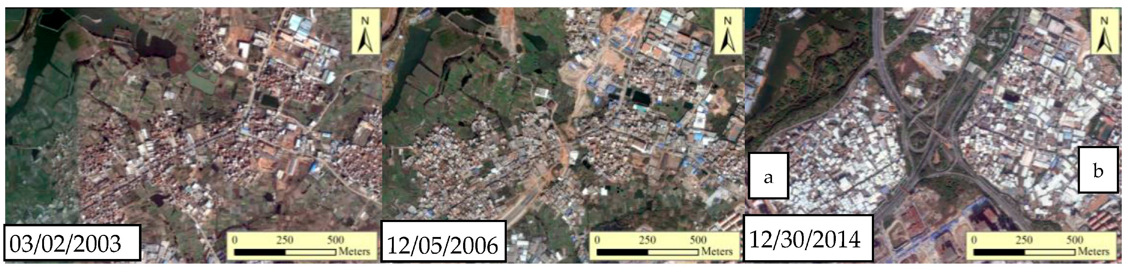
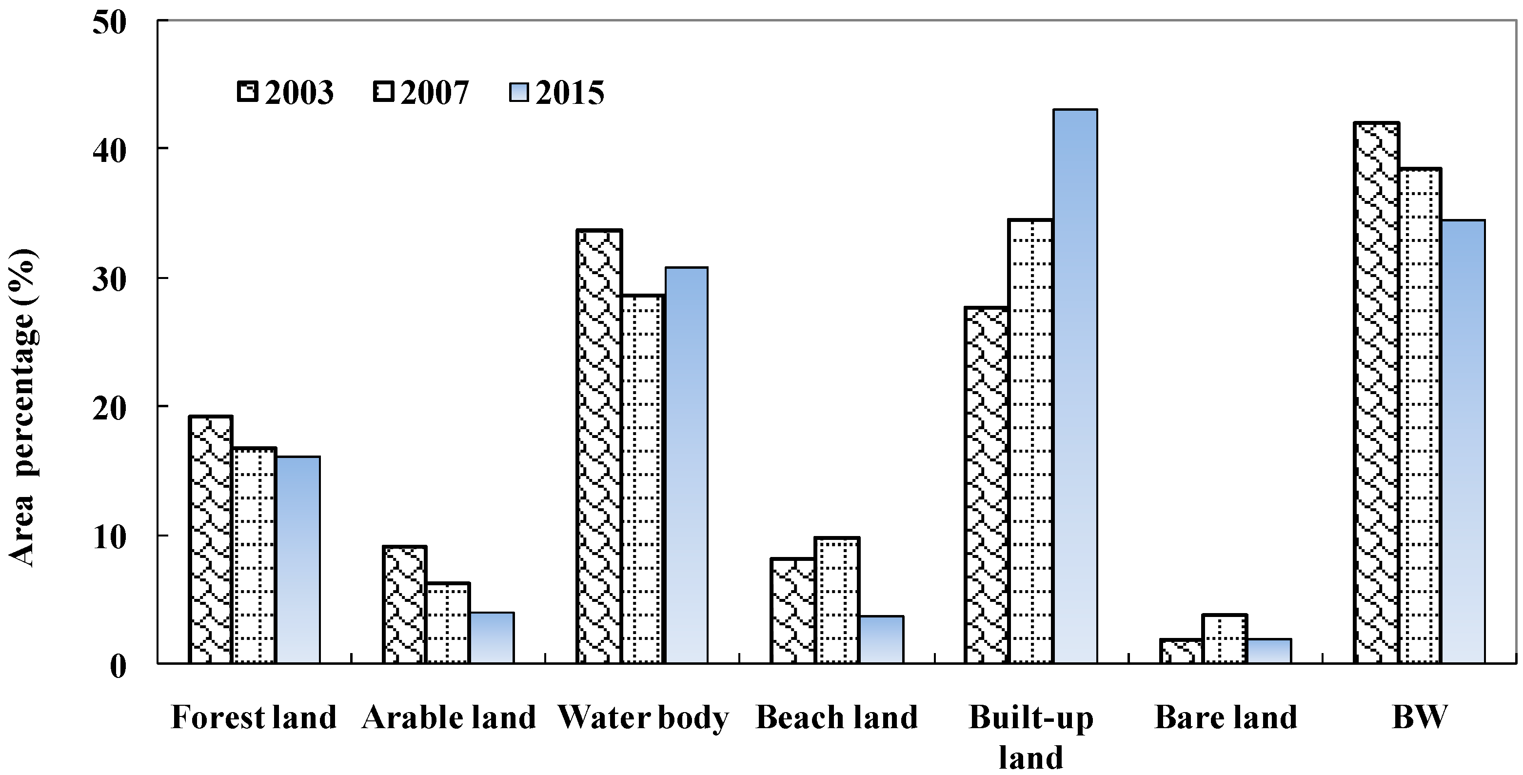
4.3. Spatiotemporal LULC Changes

Figure 9 and Figure 10 show changes in LULC distributions and area percentage in the study region from 2003 to 2015. In order to remove the influence of sea level on beach area, water bodies and beaches were merged. Among all LULC types, built-up land increased the most, from 23.67% to 43.17%, representing a 0.56-fold increase over the past 12 years. Urban land expansion was mainly achieved by occupation of coastal reclamation, arable land, and forest land. Water bodies and beaches decreased the most, from 41.98% to 34.59%. One reason for the decrease in water bodies and beaches may be related to a policy that was initiated to promote the conversion of Xiamen from an island city to a bay-like city [30]. Arable land showed the second largest decrease over the study period, from 9.13% to 4.00%. Forest land remained basically stable from 2003 to 2015. For one thing, probably because it was mostly located in hilly areas that were not suitable for urban land use. For other, forest land use was limited by a policy concerning China’s national forest city in which the green coverage rate was one of important evaluating indexes.

5. Summary and Conclusions

Monitoring the complex dynamics of cities requires consistent urban LULC maps spanning multiple time periods [3]. A variety of new techniques, in particular DTC, can help improve LULC classification and promote understanding of urban system dynamics. In this study, a FBA-DTC approach was proposed to extract urban LULC using Landsat 5 TM and Landsat 8 OLI data for a coastal city in southern China. The method’s suitability was assessed and the results were compared with those of an MLC-based approach and related studies.

Urban LULC is diverse and complex, consisting of both continuous and discrete elements, which may pose problems such as mixed pixels and spectral variability in satellite image data [15]. The FBA-DTC method is based on spectral and topographic features of image data and specialized knowledge. Images used for classification were processed with COST atmospheric correction to avoid dramatically fluctuating spectral values. The advantages of multispectral features (SAVI, NDWI, MNDBaI, BI, and WI) were combined with topographic features (DEM and Slope) and specialized knowledge to help avoid the spectral confusion to a large degree. The FBA-DTC method follows a set of clear classification rules that were constant or changed only slightly. Therefore, LULC can be rapidly and correctly classified over different time periods based on decision rules.

We obtained reference data from GE images rather than ground data because collecting ground data can be expensive and sometimes unavailable. GE images are expected to provide ground truth data and improve data visualization, and can even automatically map LULC.

The LULC classification accuracy of the FBA-DTC approach was higher than that of the MLC approach. FBA-DTC achieved an average OA of 92.13% and KC of 0.90, which were 10.17% and 0.13% higher than the MLC results, respectively. The FBA-DTC method greatly improved the classification accuracy of built-up land. The average UA for built-up land was 91.36%, which was 15.87% higher compared with the MLC results. The improved accuracy was likely due to FBA-DTC’s ability to separate bare land with light buildings from beach land and built-up land using MNDBaI and to distinguish beach land from built-up land using WI combined with elevation. Compared with other studies, the accuracy of the method presented here was satisfactory.

Our research also explored temporal changes in LULC in the study area. Built-up land showed a 0.56-fold increase over the past 12 years. The rapid extension of built-up land was mainly due to occupation of coastal reclamation, arable land, and forest land.

We developed a valuable method for quickly and objectively classifying urban LULC using parameters extracted from Landsat 5 TM and Landsat 8 OLI images with FBA-DTC. In the future, parameters should be further validated with more Landsat TM imagery and related data. It is essential to integrate other classification methods with image processing technology to improve classification accuracy. This study provides a reference for the LULC classification of coastal cities.

References

1. Lu, L.L.; Guo, H.D.; Wang, C.Z.; Pesaresi, M.; Ehrlich, D. Monitoring bidecadal development of urban agglomeration with remote sensing images in the Jing-Jin-Tang area, China. J. Appl. Remote Sens. 2014, 8, 084592. [Google Scholar] [CrossRef]
2. Grimm, N.B.; Faeth, S.H.; Golubiewski, N.E.; Wu, J.; Bai, X.M.; Briggs, J.M. Global Change and the Ecology of Cities. Science 2008, 319, 756–760. [Google Scholar] [CrossRef] [PubMed]
3. Tong, X.H.; Xie, H.; Weng, Q.H. Urban land cover classification with airborne hyperspectral data: What features to use? IEEE J. Sel. Top. Appl. 2014, 7, 3998–4009. [Google Scholar] [CrossRef]
4. Hu, T.; Yang, J.; Li, X.; Gong, P. Mapping Urban Land Use by Using Landsat Images and Open Social Data. Remote Sens. 2016, 8, 151. [Google Scholar] [CrossRef]
5. Tian, Y.; Yin, K.; Lu, D.; Hua, L.Z.; Zhao, Q.J.; Wen, M.P. Examining Land Use and Land Cover Spatiotemporal Change and Driving Forces in Beijing from 1978 to 2010. Remote Sens. 2014, 6, 10593–10611. [Google Scholar] [CrossRef]
6. Elatawneh, A.; Kalaitzidis, C.; Petropoulos, G.P.; Schneider, T. Evaluation of diverse classification approaches for land use/cover mapping in a Mediterranean region utilizing Hyperion data. Int. J. Digit. Earth 2014, 7, 194–216. [Google Scholar] [CrossRef]
7. Davranche, A.; Lefebvre, G.; Poulin, B. Wetland monitoring using classification trees and SPOT-5 seasonal time series. Remote Sens. Environ. 2010, 114, 552–562. [Google Scholar] [CrossRef] [Green Version]
8. Mathieu, R.; Aryal, J. Object-based classification of Ikonos imagery for mapping large-scale vegetation communities in urban areas. Sensors 2007, 7, 2860–2880. [Google Scholar] [CrossRef] [PubMed]
9. Lu, D.; Hetrick, S.; Moran, E. Land cover classification in a complex urban-rural landscape with quickbird imagery. Photogramm. Eng. Remote Sens. 2010, 76, 1159–1168. [Google Scholar] [CrossRef]
10. Jawak, S.D.; Luis, A.J. Improved land cover mapping using high resolution multiangle 8-band WorldView-2 satellite remote sensing data. J. Appl. Remote Sens. 2013, 7, 073573. [Google Scholar] [CrossRef]
11. Fauvel, M.; Benediktsson, J.A.; Chanussot, J.; Sveinsson, J.R. Spectral and spatial classification of hyperspectral data using SVMs and morphological profiles. IEEE Trans. Geosci. Remote Sens. 2008, 46, 3804–3814. [Google Scholar] [CrossRef]
12. Guo, H.; Huang, Q.; Li, X.; Sun, Z.; Zhang, Y. Spatiotemporal analysis of urban environment based on the vegetation–impervious surface–soil model. J. Appl. Remote Sens. 2014, 8, 084597. [Google Scholar] [CrossRef]
13. Yuan, H.; Van Der Wiele, C.F.; Khorram, S. An automated artificial neural network system for land use/land cover classification from Landsat TM imagery. Remote Sens. 2009, 1, 243–265. [Google Scholar] [CrossRef]
14. Gopal, S.; Tang, X.J.; Phillips, N.; Nomack, M.; Pasquarella, V.; Pitts, J. Characterizing urban landscapes using fuzzy sets. Comput. Environ. Urban Syst. 2016, 57, 212–223. [Google Scholar] [CrossRef]
15. Petropoulos, G.P.; Vadrevu, K.P.; Kalaitzidis, C. Spectral angle mapper and object-based classification combined with hyperspectral remote sensing imagery for obtaining land use/cover mapping in a Mediterranean region. Geocarto Int. 2013, 28, 114–129. [Google Scholar] [CrossRef]
16. Lo, C.P.; Choi, J. A hybrid approach to urban land use/cover mapping using Landsat 7 Enhanced Thematic Mapper Plus (ETM+) images. Int. J. Remote Sens. 2004, 25, 2687–2700. [Google Scholar] [CrossRef]
17. Wentz, E.A.; Nelson, D.; Rahman, A.; Stefanov, W.L.; Roy, S.S. Expert system classification of urban land use/cover for Delhi, India. Int. J. Remote Sens. 2008, 29, 4405–4427. [Google Scholar] [CrossRef]
18. Pal, M.; Mather, P.M. An assessment of the effectiveness of decision tree methods for land cover classification. Remote Sens. Environ. 2003, 86, 554–565. [Google Scholar] [CrossRef]
19. Wang, C.; Liu, H.Y.; Zhang, Y.; Li, Y.F. Classification of land-cover types in muddy tidal flat wetlands using remote sensing data. J. Appl. Remote Sens. 2013, 7, 073457. [Google Scholar] [CrossRef]
20. Punia, M.; Joshi, P.K.; Porwal, M.C. Decision tree classification of land use land cover for Delhi, India using IRS-P6 AWiFS data. Expert Syst. Appl. 2011, 38, 5577–5583. [Google Scholar] [CrossRef]
21. Baker, C.; Lawrence, R.; Montagne, C.; Patten, D. Mapping wetlands and riparian areas using Landsat ETM+ imagery and decision-tree-based models. Wetlands 2006, 26, 465–474. [Google Scholar] [CrossRef]
22. Otukei, J.R.; Blaschke, T. Land cover change assessment using decision trees, support vector machines and maximum likelihood classification algorithms. Int. J. Appl. Earth Obs. Geoinf. 2010, 12, S27–S31. [Google Scholar] [CrossRef]
23. Sesnie, S.E.; Gessler, P.E.; Finegan, B.; Thessler, S. Integrating Landsat TM and SRTM–DEM derived variables with decision trees for habitat classification and change detection in complex neotropical environments. Remote Sens. Environ. 2008, 112, 2145–2159. [Google Scholar] [CrossRef]
24. Tooke, T.R.; Coops, N.C.; Goodwin, N.R.; Voogt, J.A. Extracting urban vegetation characteristics using spectral mixture analysis and decision tree classifications. Remote Sens. Environ. 2009, 113, 398–407. [Google Scholar] [CrossRef]
25. Kandrika, S.; Roy, P.S. Land use land cover classification of Orissa using multi-temporal IRS-P6 awifs data: A decision tree approach. Int. J. Appl. Earth Obs. Geoinf. 2008, 10, 186–193. [Google Scholar] [CrossRef]
26. Qi, Z.; Yeh, A.G.O.; Li, X.; Lin, Z. A novel algorithm for land use and land cover classification using RADARSAT-2 polarimetric SAR data. Remote Sens. Environ. 2012, 118, 21–39. [Google Scholar] [CrossRef]
27. Powell, R.L.; Roberts, D.A.; Dennison, P.E.; Hess, L.L. Subpixel mapping of urban land cover using multiple endmember spectral mixture analysis: Manaus, Brazil. Remote Sens. Environ. 2007, 106, 253–267. [Google Scholar] [CrossRef]
28. He, C.Y.; Shi, P.J.; Xie, D.Y.; Zhao, Y.Y. Improving the normalized difference built-up index to map urban built-up areas using a semiautomatic segmentation approach. Remote Sens. Lett. 2010, 1, 213–221. [Google Scholar] [CrossRef]
29. Khatami, R.; Mountrakis, G.; Stehman, S.V. A meta-analysis of remote sensing research on supervised pixel-based land-cover image classification processes: General guidelines for practitioners and future research. Remote Sens. Environ. 2016, 177, 89–100. [Google Scholar] [CrossRef]
30. Lin, T.; Xue, X.; Shi, L.; Gao, L. Urban spatial expansion and its impacts on island ecosystem services and landscape pattern: A case study of the island city of Xiamen, Southeast China. Ocean Coast. Manag. 2013, 81, 90–96. [Google Scholar] [CrossRef]
31. Tang, L.N.; Zhao, Y.; Yin, K.; Zhao, J. City profile: Xiamen. Cities 2013, 31, 615–624. [Google Scholar] [CrossRef]
32. Hua, L.Z.; Li, X.Q.; Tang, L.N.; Yin, K.; Zhao, Y. Spatio-temporal dynamic analysis of island-city landscape: A case study of Xiamen Island, China. Int. J. Sustain. Dev. World Ecol. 2010, 17, 273–278. [Google Scholar] [CrossRef]
33. Hua, L.Z.; Tang, L.N.; Cui, S.H.; Yin, K. Simulating Urban Growth Using the SLEUTH Model in a Coastal Peri-Urban District in China. Sustainability 2014, 6, 3899–3914. [Google Scholar] [CrossRef]
34. Hao, P.; Sliuzas, R.; Geertman, S. The development and redevelopment of urban villages in Shenzhen. Habitat Int. 2011, 35, 214–224. [Google Scholar] [CrossRef]
35. Chavez, P.S. Image-based atmospheric corrections—Revisited and revised. Photogramm. Eng. Remote Sens. 1996, 62, 1025–1036. [Google Scholar]
36. Wu, J.; Wang, D.; Bauer, M.E. Image-based atmospheric correction of QuickBird imagery of Minnesota cropland. Remote Sens. Environ. 2005, 99, 315–325. [Google Scholar] [CrossRef]
37. Lu, D.; Mausel, P. Assessment of atmospheric correction methods applicable to Amazon basin LBA research. Int. J. Remote Sens. 2002, 23, 2651–2671. [Google Scholar] [CrossRef]
38. Huete, A.R. A Soil-adjusted vegetation index (SAVI). Remote Sens. Environ. 1988, 25, 295–309. [Google Scholar] [CrossRef]
39. McFeeters, S.K. The use of the Normalized Difference Water Index (NDWI) in the delineation of open water features. Int. J. Remote Sens. 1996, 17, 1425–1432. [Google Scholar] [CrossRef]
40. Zhao, H.M.; Chen, X.L. Use of normalized difference bareness index in quickly mapping bare areas from TM/ETM+. In Proceedings of the 2005 IEEE International Geoscience and Remote Sensing Symposium, Seoul, Korea, 25–29 July 2005; pp. 1666–1668. [Google Scholar]
41. Kauth, R.J.; Thomas, G.S. The tasseled cap—A graphic description of the spectral-temporal development of agricultural crops as seen by Landsat. In Proceedings of the Symposium on Machine Processing of Remotely Sensed Data, Purdue University, West Lafayette, IN, USA, 29 June–1 July 1976. [Google Scholar]
42. Crist, E.P. A TM tasseled cap equivalent transformation for reflectance factor data. Remote Sens. Environ. 1985, 17, 301–306. [Google Scholar] [CrossRef]
43. Baig, M.H.; Zhang, L.; Shuai, T.; Tong, Q. Derivation of a tasselled cap transformation based on Landsat 8 at-satellite reflectance. Remote Sens. Lett. 2014, 5, 423–431. [Google Scholar] [CrossRef]
44. Biradar, C.M.; Thenkabail, P.S.; Noojipady, P.; Li, Y.; Dheeravath, V.; Turral, H.; Velpuri, M.; Gumma, M.K.; Gangalakunta, O.R.; Cai, X.L.; et al. A global map of rainfed cropland areas (GMRCA) at the end of last millennium using remote sensing. Int. J. Appl. Earth Obs. Geoinf. 2009, 11, 114–129. [Google Scholar] [CrossRef]
45. Hu, Q.; Wu, W.; Xia, T.; Yu, Q.; Yang, P.; Li, Z.; Song, Q. Exploring the use of Google Earth imagery and object-based methods in land use/cover mapping. Remote Sens. 2013, 5, 6026–6042. [Google Scholar] [CrossRef]
Figure 1. Location of the study area (red box) in 2007; the blue area is the sea.
Ijgi 06 00331 g001
Figure 2. Flow chart used in the research. Notes: FBA-DTC is feature-based approach of decision tree classification; SAVI is soil adjusted vegetation index; NDWI is normalized difference water index; NDBaI is normalized difference barren index; MNDBaI is modified normalized difference barren Index; BI is brightness index; WI is wetness index.
Ijgi 06 00331 g002
Figure 3. Feature-based approach of decision tree classification constructed to extract urban LULC using Landsat 5 TM and Landsat 8 OLI data (see Figure 2 for key to abbreviations).
Ijgi 06 00331 g003
Figure 4. Increase of white tin roofs in two urban villages, Gaolin (a) and Wutong (b) of Xiamen island, obtained from Google Earth from 2003 to 2014.
Ijgi 06 00331 g004
Figure 5. Spectral profiles of typical land use and land cover types in the study area in 2007.
Ijgi 06 00331 g005
Figure 6. Comparison of original images with undistinguishable fallow land and built-up land, and an arable land map: (a) original image in 2003; (b) original image in 2007; (c) arable land map extracted from feature-based approach of decision tree classification in 2003. Notes: A and B represent built-up land and fallow land; CL and FL stand for cropland and fallow land.
Ijgi 06 00331 g006
Figure 7. Wetness index versus area percentage of beaches.
Ijgi 06 00331 g007
Figure 8. Brightness index versus area percentage of arable land.
Ijgi 06 00331 g008
Figure 9. LULC classification results. (a) Feature-based approach of decision tree classification (FBA-DTC) applied to the image from 2015; (b) MLC applied to the image from 2015; (c) FBA-DTC applied to the image from 2007; (d) MLC applied to the image from 2007; (e) FBA-DTC applied to the image from 2003; (f) MLC applied to the image from 2003.
Ijgi 06 00331 g009aIjgi 06 00331 g009b
Figure 10. LULC changes in the study area from 2003 to 2015. Note: BW is the sum of beach land and water bodies.
Ijgi 06 00331 g010